Air–sea interaction heat and momentum fluxes based on vessel's experimental observations over Spanish waters

The ocean and atmosphere communicate directly through air–sea interaction fluxes. These include heat exchange by latent (LHFL) and sensible (SHFL) heat and momentum (MOFL) by wind stress. These stand as the leading predictors of how the ocean influences atmospheric variability and vice versa. In this paper, meteorological and upper-ocean measurements collected during the period of 2011–2023 aboard four research vessels over Spanish waters and adjacent seas are used to study air–sea interaction fluxes. These research vessels are Ramón Margalef (RM), Ángeles Alvariño (AJ), and Cornide de Saavedra (CS) belonging to the Instituto Español de Oceanografía (IEO-CSIC) and Miguel Oliver (MO) of the Secretaría General de Pesca of Spain. Recorded data are sent daily to the IEO Data Center on land, where quality control procedures are applied. Heat and momentum flux products are derived using the bulk aerodynamic approximation and are stored within a MEDAR/MedAtlas format alongside the meteorological and ocean variables used in the calculation. The data sets generated and described here are publicly available at SEANOE (https://doi.org/10.17882/103856, Sánchez-Lorente and Tel, 2024a; https://doi.org/10.17882/103424, Sánchez-Lorente and Tel, 2024b; https://doi.org/10.17882/103903, Sánchez-Lorente and Tel, 2024c; https://doi.org/10.17882/103855, Sánchez-Lorente and Tel, 2024d). In order to study the behaviour of these air–sea fluxes, several marine-region subdivisions, based on the heterogeneity of the Spanish waters, are proposed. Additionally, some results within the context of these regions are shown.

1 Introduction

The ocean and atmosphere maintain a close and constant relationship through numerous processes that are responsible for countless effects on different scales, from the general circulation of both media to the formation of convective air masses by turbulent processes in the atmospheric boundary layer (ABL) (Large and Pond, 1981). The study of these phenomena must focus on air–sea interactions occurring at the interface of both subsystems, commonly known as heat and momentum turbulent fluxes. The former refers to sensible and latent fluxes, which account for the loss of heat by the sea due to convection and evaporation, respectively, while the latter is governed by the wind stress at the sea surface. A deeper understanding of the temporal behaviour, spatial distribution, or climatological tendencies will enable a further improvement in understanding the climate system and its variability (Ruiz et al., 2008).

The experimental record of these magnitudes is generally scarce. Direct measurement requires very costly and technologically demanding equipment, which can be substituted by several approximations and parameterisations that have been developed and studied on offshore platforms, buoys, and vessels in the open ocean since the latest decades of the 20th century (Smith, 1980; Large and Pond, 1981, 1982; Grachev and Fairall, 1997; Edson et al., 2013; Zhang et al., 2024). In most cases, the main purpose of these studies was to calibrate and test the different methods for estimating turbulent fluxes at the air–sea interface under various weather and sea conditions. The experimental record, nevertheless, implies several drawbacks, such as data-sampling density, short data series, incomplete spatial coverage, or systematic measurement errors.

Recently, other alternative procedures have been developed to better capture air–sea interactions. In this context, satellite-based flux products (Yu and Weller, 2007) have enabled improvements in temporal and spatial resolutions, as well as enhanced global coverage; see, for example, the studies of Kubota et al. (2002) and Bentamy et al. (2003) for sensible and latent fluxes and the study of O'Neill (2012) for wind stress. However, these products are not independent of field measurements due to the need for validation and other calibration procedures. Additionally, they present certain technical difficulties, making them less reliable to derive variables like specific humidity and air temperature, which ultimately affect heat flux outcomes. On the contrary, wind stress is well represented thanks to the finer temporal and spatial resolution and the reduced uncertainties related to record errors (Pierson Jr, 1990). Furthermore, new modelling-based products from various climate research organisations around the world have contributed to the study of global air–sea variability and its implications, reducing the constraints of field measurements by combining, through statistical analysis processes, the information from numerous monitoring sources (e.g, satellite, buoys, ships, reanalysis). Notable air–sea interaction products with global coverage include the NCEP Climate Forecast System Reanalysis (CFSR), Objectively Analyzed Air-Sea Fluxes (OAFlux) (Yu and Weller, 2007), the Modern-Era Retrospective Analysis for Research and Applications (MERRA) (Bosilovich, 2008), and the SeaFlux data product (Curry et al., 2004). However, due to the different analysis processes and the use of independent data sources, these exhibit discrepancies and biases, unveiling the need for further improvement of the validation of bulk variables (Bentamy et al., 2017). As an example, turbulent flux behaviours appear to be more homogeneous in tropical latitudes compared to in mid-latitude and subpolar regions across several analysis products. Additionally, OAFlux and NCEP show great biases in complex circulation areas (Mao et al., 2021), as well as seasonal biases (Zhou et al., 2018), which must be taken into account prior to any subsequent analysis.

Concerning waters in the Mediterranean and Cantabrian–Atlantic areas, there is also previous research based on dynamical downscaling of the NCEP/NCAR global reanalysis (HIPOCAS) (Vargas-Yáñez et al., 2007; Ruiz et al., 2008). It achieves a spatial resolution of 0.5°×0.5° in the Mediterranean Sea during a 44-year period between 1958–2001. It follows the line of other authors focused on this basin (Bunker et al., 1982; Garrett et al., 1993; Castellari et al., 1998), improving the representation of regional aspects of heat fluxes thanks to its reanalysis methodology. Nevertheless, different resolutions and model configurations introduce biases and discrepancies that require observational data for their validation.

In this line, this paper presents the air–sea interaction fluxes obtained from meteorological and thermosalinograph (TSG) experimental records during the period of 2011–2023 aboard four research vessels: Ramón Margalef (RM), Ángeles Alvariño (AJ), Miguel Oliver (MO), and Cornide de Saavedra (CS). These air–sea interaction fluxes are sensible and latent heat fluxes (SHFLs and LHFLs, respectively) and momentum flux (MOFL), also known as wind stress. AJ and RM are part of the current fleet of the Instituto Español de Oceanografía (IEO-CSIC), whereas CS is a former vessel that is currently decommissioned. MO belongs to the Secretaría General de Pesca of Spain. These multidisciplinary research vessels are equipped with state-of-the-art technological equipment for navigation and for scientific research. Despite the specific objectives of each cruise, continuous meteorological and TSG data are collected during their trajectories and activities. Generally, monitoring sensors are switched off when arriving at port for preservation and maintenance. However, the high sample frequency during their activities allows us to establish continuous temporal series throughout the entirety of the vessels' trajectories.

The paper is organised as follows: firstly, in Sect. 2, a description of the marine areas covered by the vessel's trajectories is shown. Next, in Sect. 3, the description of the data records, the validation and quality control (QC) procedures for the different data sources, and the methodology employed in the calculation of air–sea fluxes are explained. Some results and a discussion are presented in Sect. 4. Additionally, the availability and accessibility of the data are detailed in Sect. 5. Finally, a conclusion is provided in the last section.

2 Study area

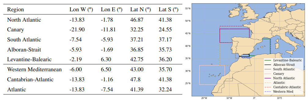
During their activities and trajectories, the AJ, RM, MO, and CS vessels cover a large part of the Spanish waters and adjacent seas. These are notoriously heterogeneous waters, ranging from subtropical to mid-latitude zones. They present different ranges of temperature and salinity due to the constrictions of continental distribution around the specific areas, e.g. with the semi-enclosed regime of the warm and salty Mediterranean sea in comparison with the open and colder waters of the Cantabrian Sea at higher latitudes or with the subtropical waters of the Canary Islands region (Talley, 2011). Also, different regional wind regimes, crucial for air–sea interaction, are characteristic of each region (Viedma Muñoz, 2005; Azorin-Molina et al., 2018; Ortega et al., 2023). Thus, the ocean–atmosphere interaction processes present disparities depending on the oceanographic and meteorological characteristics of each location. Therefore, prior to any scientific analysis, such heterogeneity encourages a solid and well-founded subdivision in pertinent marine regions. In Fig. 1, several subdivisions around the Spanish marine territory are proposed. The first five, the North Atlantic, Canary, South Atlantic, Alboran-0Strait, and Levantine–Balearic, are part of the Spanish jurisdictional waters. They are also known as marine demarcations, defined by the Marine Strategy Framework Directive from the EU (Long, 2011) for protection and preservation purposes to prevent marine ecosystems from deteriorating. Additionally, three more regions are offered: the western Mediterranean, which covers the Alboran–Strait and Levantine–Balearic areas; the Cantabrian–Atlantic, which involves the North Atlantic region alongside the northern waters of the Vizcaya Gulf; and the Atlantic, which extends from the coast of Portugal to the margins of Africa and the Canary Islands region.

Figure 1 Marine subdivisions of the different areas covered by the AJ, RM, MO, and CS vessel trajectories. Geographical limits are specified. The top five regions belong to the Spanish jurisdictional waters defined by the Marine Strategy Framework Directive from the EU (Long, 2011).

3 Methodology

3.1 Data records

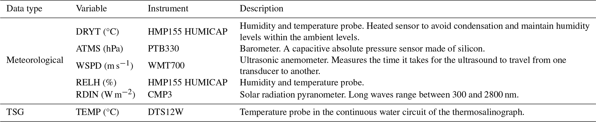
Four vessels' data records are used to obtain the air–sea interaction fluxes. The AJ, RM, MO, and CS research vessels are provided with meteorological and sea surface monitoring equipment, allowing them to measure the variables required to obtain the final flux products throughout their trajectories. The onboard measuring instrumentation is a Vaisala AWS430 unit, specifically designed to measure climatological variables within a marine environment. Information about the instruments used for the measurement of each magnitude is detailed in Table 1. The variables recorded during the period of 2011–2023 and stored within this data set are air temperature (DRYT), atmospheric pressure (ATMS), wind speed (WSPD), relative humidity (RELH), and total incident radiation (RDIN), recorded by the meteorological equipment, and sea temperature (TEMP), recorded using the TSG. The names of the variables and their descriptions follow the standards of the MedAtlas Parameter Usage Vocabulary from the British Oceanographic Data Centre (BODC), which can be further explored at https://vocab.seadatanet.org/search (last access: 15 October 2025).

Table 1 Vaisala AWS430 meteorological and TSG instrumentation aboard the research vessels for the experimental record.

Daily, both types of data, meteorological and TSG, are sent to the IEO Data Center on land and kept within archives for each month and vessel. Then, formatting and quality control (QC) procedures are applied for its permanent storage within MEDAR/MedAtlas format (Maillard et al., 1998). MEDAR/MedAtlas is an ASCII auto-descriptive format available since the last decade of the 20th century, which merges to facilitate reading, recording, processing, and storing oceanographic data. Each file is provided with a heading where all metadata information is reflected alongside a flag column where the QC labels are specified. Data sampling has a different frequency for each type of data. In consequence, final flux products are calculated at an hourly frequency. Then, with all of the information above having been gathered, final MEDAR/MedAtlas formatted heat and momentum flux data archives are constructed (also following BODC vocabulary standards) for each month and vessel (Sánchez-Lorente and Tel, 2024a, b, c, d). The columns in these archives show the three air–sea interaction fluxes, SHFL, LHFL, and MOFL, along with the variables used in their calculation (which are shown in Table 1). A flag column is also added based on the criteria specified in the QC section. Besides this, incident radiation (RDIN) is also included in order to bring about the possibility to determine the total heat storage (HS) in the ocean (Eq. 1):

$$\begin{array}{}\text{(1)}& \mathrm{HS}=Q_{\mathrm{s}}+Q_{\mathrm{lw}}+\mathrm{SHFL}+\mathrm{LHFL},\end{array}$$

where Q_s is the shortwave incident radiation from the sun, and Q_lw is the net longwave radiation. RDIN accounts for both shortwave and longwave incident radiation from the sun and atmosphere. The upward longwave radiation from the sea can be obtained with the Stefan–Boltzmann radiation law using the sea temperature (TEMP) through R=ϵσT⁴ (Stull, 2012), where ϵ is the emissivity ranging between 0.93 and 1 (Fung et al., 1984), and σ is the Stefan–Boltzmann constant. Thus, Q_s and Q_lw are addressed by the data set, and, alongside the air–sea interaction heat fluxes, both radiative and convective exchanges between the two media are determined.

3.2 Validation and QC

In order to obtain reliable data products, it is important to elaborate on adequate validation and QC procedures. Both types of records (meteorological and TSG data, as well as subsequent flux products) are revised and checked by manual and automatic techniques. As was previously mentioned, all MEDAR/MedAtlas archives contain a flag column that specifies the QC of each variable and individual data sample. The flag criteria are based on SeaDataNet guidelines (Schaap and Lowry, 2010).

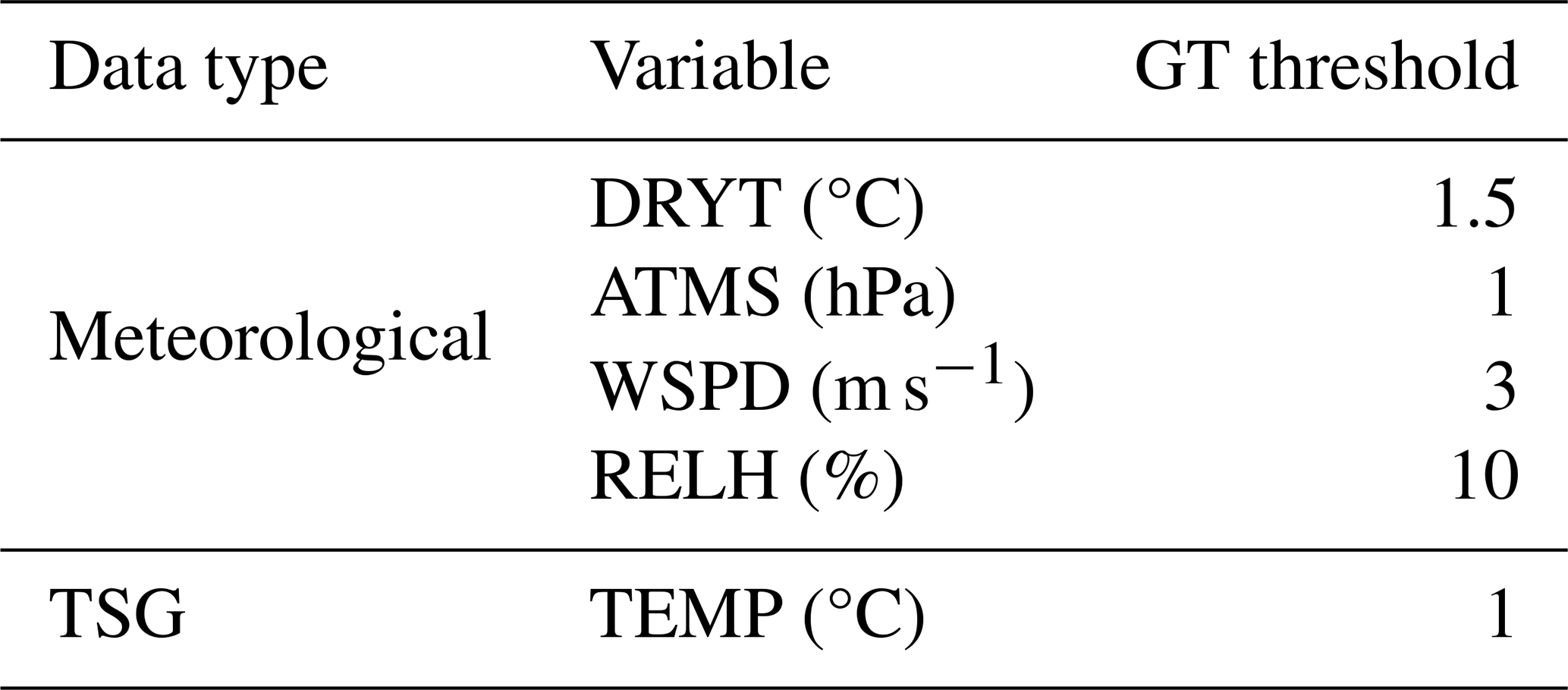
Firstly, meteorological and TSG data are validated by visual inspection, which is useful to check the reliability of the data set. This enables us to understand the noise of the time series while simultaneously identifying immediate anomalous or spike records. Thus, the time series of each year's data records for each data type is represented, allowing us to observe whether all measurements are within the temporal limits specified in the metadata heading. In addition, map plotting of the vessel's trajectories is a practical procedure to detect position errors. Additionally, other automatic processes are executed. A global range test for each variable is conducted by setting highly extreme thresholds, which would be impossible to exceed in real life: e.g. >100 % or negative values for relative humidity. Also, more restrictive limits are fixed, taking into account regional and seasonal climatological behaviours. The North Atlantic area does not reach such high sea surface and air temperature values as the western Mediterranean or Canary regions. Furthermore, additional QC tests are applied based on SeaDataNet recommendations (Schaap and Lowry, 2010). A gradient test (GT), represented by Eq. (2), which evaluates if the gradient of a measurement and the previous and next values is too sharp, is applied for each variable:

$$\begin{array}{}\text{(2)}& \mathrm{GT}=|V_{\mathrm{2}}-\left(V_{\mathrm{3}}+V_{\mathrm{1}}\right)/\mathrm{2}|,\end{array}$$

where V₂  is the record being checked, and V₁ and V₃ are the previous and next measurements. If GT is higher than the values specified in Table 2, it is flagged as 4.

Table 2 GT thresholds used for each variable during the QC process.

Temperature data are also tested under a spike test (ST) following Eq. (3):

$$\begin{array}{}\text{(3)}& \mathrm{ST}=|V_{\mathrm{2}}-\left(V_{\mathrm{3}}+V_{\mathrm{1}}\right)/\mathrm{2}|-|\left(V_{\mathrm{3}}-V_{\mathrm{1}}\right)/\mathrm{2}|.\end{array}$$

SeaDataNet guidelines fix the ST at 6 °C (if ST > 6 °C, V₂ fails the test). However, noticing the large threshold this quantities supposes, another fixed limit is implemented based on statistical analysis (Paladini de Mendoza et al., 2022). This new threshold is calculated to be 3 times the interquartile range (IQR) parameter (3 × IQR); the IQR is defined based on the first (Q₁) and third (Q₃) quantiles of the monthly distribution: IQR = Q₃−Q₁. The most restrictive threshold, 6 °C or 3 × IQR, is the reference for each test. Lastly, additional QC procedures are applied: if a constant value is repeated notably during the record, it is flagged as 4, and, even if, under all of the tests applied, there exist notorious eye-catching spike values to remove, they are also flagged manually as 4 based on the expertise developed throughout the study. Regarding the final flux data set, if any of the meteorological or TSG variables involved in the calculation are flagged with a value other than 1, the air–sea interaction fluxes are automatically flagged in the same way. In addition, flux time series and map trajectories are newly checked in order to, firstly, confirm that all data are placed over the sea and, secondly, identify any prominent spikes which are then flagged manually.

The time period covered by this study is 2011–2023. However, the data record is not a continuous and uninterrupted time series. Data records are collected based on the availability of the ship's activities. Additionally, technical problems or preventative actions to maintain its good condition might turn the experimental equipment off, creating gaps in the record. This, along with the QC procedures, reduces the amount of valid data available (Fig. 2).

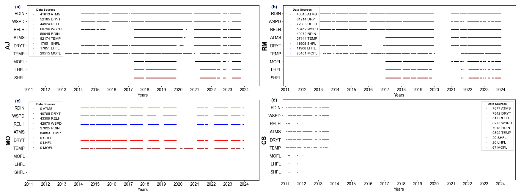
Figure 2 Quality-controlled data record timeline from 2011 to 2023 for each meteorological and TSG variable, as well as for SHFL, LHFL, and MOFL products for each vessel: AJ (a), RM (b), MO (c), and CS (d). The size of data sample for each variable is indicated in the plot legend.

3.3 Air–sea interaction flux calculation

Air–sea, heat, and momentum fluxes are transmitted to the surface layer (SL), the layer immediately closest to the interface between the atmosphere and ocean and the lowest layer in the ABL (Stull, 2012). Here, the turbulent exchange within both media, its dynamics, and its implications for the development of the ABL are ruled by Monin–Obukhov similarity theory (Foken, 2006), which ensures that these heat and momentum fluxes are constant with height. Mentioned fluxes are transported by the vertical wind component ω. Hence, sensible and latent heat fluxes can be considered to be temperature and humidity fluxes into the atmosphere, whereas the momentum flux appears as wind stress towards the surface. The experimental measurement of these quantities requires a temporal resolution that is enough to capture the turbulent fluctuations – or eddies – of the magnitudes immersed in these transports. Several experimental approaches exist to determine these quantities, e.g. the eddy correlation method (Large and Pond, 1982) or the dissipation method (Pond et al., 1971). However, the most useful methodology to calculate the mentioned turbulent fluxes, which is used in this study due to the experimental and technical constraints, is the bulk aerodynamic approximation (Grachev and Fairall, 1997) (Eqs. 4–6). Here, a relationship between air–sea fluxes and the gradient of temperature, specific humidity, and horizontal wind, respectively, is established between the sea surface and the corresponding measurement point in the atmosphere:

$$\begin{array}{}\text{(4)}& {\displaystyle }\mathrm{SHFL}=\mathit{\rho }{C}_{\mathrm{p}}{C}_{\mathrm{T}}U\left(z\right)\left(T_{\mathrm{s}}-T_{\mathrm{a}}\left(z\right)\right),\text{(5)}& {\displaystyle }\mathrm{LHFL}=\mathit{\rho }L{C}_{\mathrm{E}}U\left(z\right)\left(q_{\mathrm{s}}-q_{\mathrm{a}}\left(z\right)\right),\text{(6)}& {\displaystyle }\mathrm{MOFL}=\mathit{\rho }{C}_{\mathrm{D}}{U}^{\mathrm{2}}\left(z\right),\end{array}$$

where the subindex “s” references the sea surface, whereas “a” references the atmosphere; ρ is the air density; C_p and L are the specific heat at constant pressure and the latent heat of evaporation, respectively; U is the wind speed; T and q are the temperature and the specific humidity of the media; and C_T, C_E, and C_D are aerodynamic bulk coefficients. Following these criteria, SHFL to the atmosphere is positive if sea temperature is higher than air temperature, whilst LHFL is positive when there is evaporation. MOFL is always positive due to the wind stress from the atmosphere to the sea surface. In ideal conditions, U(z) is the wind speed relative to the sea surface current, which can be measured using specific equipment such as scatterometers (Edson et al., 2013; Chacko et al., 2022). In this case, ultrasonic anemometers are used to measure wind speed and direction, unable to determine the sea current speed. Thus, U(z) is considered henceforth to be the absolute wind velocity, neglecting the effects of the surface ocean current. Previous studies have pointed to errors of between 10 %–20 % when neglecting ocean currents around 0.5 m s⁻¹ (Trenberth et al., 1990).

C_T and C_E are the aerodynamic heat and moisture coefficients, respectively. They depend on the stability of the SL, as well as the wind speed. Several researches have found values of C_T between $\mathrm{1.1}\times {\mathrm{10}}^{-\mathrm{3}}$ for unstable stratification and $\mathrm{0.75}\times {\mathrm{10}}^{-\mathrm{3}}$ in a stable atmosphere (Smith, 1980). On the contrary, for C_E, Anderson and Smith (1981) conclude that it depends more on wind speed than on stability. Hence, for this study, due to the limitation in obtaining the state of the stability of the ABL (it would be essential to calculate the characteristic turbulent scales of temperature, wind, and moisture according to Monin–Obukhov theory), the bulk aerodynamic coefficients are considered to be constants: $\mathrm{1}\times {\mathrm{10}}^{-\mathrm{3}}$ for C_T (Pond et al., 1971) and $\mathrm{1.3}\times {\mathrm{10}}^{-\mathrm{3}}$ for C_E (Anderson and Smith, 1981). Furthermore, for the drag coefficient C_D, the wind dependency relation exposed in Large and Pond (1981) and implemented in the Python Air–Sea routines (https://github.com/pyoceans/python-airsea, last access: 15 October 2025) is used. The air density ρ is calculated using the ideal-gas equation (Iribarne and Godson, 2012). The specific humidity is derived from the pressure and relative humidity measurements. It is calculated using the specific humidity in saturated conditions based on the vapour pressure dependency on temperature as identified by Buck (1981), which is also addressed by the aforementioned Air–Sea routines, and the relation $\mathrm{RH}=q/q_{\mathrm{saturated}}$, with RH representing the relative humidity. The specific humidity of the sea surface q_a is obtained analogously but considering saturation conditions. This is multiplied by a factor of 0.98 due to the reduction in saturated vapour pressure as a consequence of salt concentration (Large and Yeager, 2009). Specific heat at constant pressure C_p has a value of 1004.7 J kg⁻¹ K⁻¹, whereas the latent heat of evaporation amounts to 2.5×10⁶ J kg⁻¹.

For these calculations, the availability of the meteorological and TSG variables measurements is needed. The absence of any variable involved in Eqs. (4)–(6) makes it impossible to determine SHFL, LHFL, and MOFL. For the period from 2013 to 2016, there are no pressure measurements from the AJ, RM, and/or MO vessels (Fig. 2). This also happens during the rest of the years for MO. Nonetheless, the data are still useful to determine the sign of the fluxes (difference in terms of temperature or humidity between ocean and atmosphere, as in Eqs. 4and 5). Given that, despite the fact that the concrete value cannot be obtained, its tendency, proportionality, and behaviour can still be inferred.

4 Results and discussion

4.1 Outcome availability

Once the QC is applied and the data are in a well-suited MEDAR/MedAtlas format, results and analysis from AJ, RM, MO, and CS measurements can be obtained. During their oceanographic activities, the vessels cover a notorious area near the Spanish waters (Fig. 3a). The total sum of the entire data sampling between 2011 and 2023 is 211 713 rows of meteorological and TSG data and their subsequent air–sea flux products. However, the measurements flagged with 9 and 4 (meaning no data and error data, respectively) reduce the operative number of data available for each variable. In Table 3, the number (and percentage) flagged as “good value” (1) for each variable is shown, whereas, in Table 4, the flux products flagged as 4 for each marine region are specified. The atmospheric pressure is the variable with fewer good values (44.6 %) due to the lack of measurements during the period of 2013–2016 by the AJ, RM, and MO vessels, although this accounts for a significant number of 94 572 values. This is followed by the sea temperature (62.7 %), which directly affects the heat fluxes; this is the reason why there exists such a remarkable difference between the percentage of heat (14.1 %) and momentum (25.8 %) fluxes. The absence of good values of RELH stands out mainly during the CS's trajectories between 2011 and 2013, when values above 100 % and below 0 %, which prevent the correct determination of the air density, are recorded; however, its percentage of good values is a notorious 76.5 %. Also, some slightly disproportionate wind speed measurements recorded by CS are flagged as 4; nonetheless, it presents a high percentage of good values. Furthermore, DRYT exceeds these percentages, with 77.5 %, despite presenting occasional high values registered during the winter months in 2018 and 2019.

Table 3 Number (and percentage) of good values (data flagged as 1) for each variable within the total of the four vessels' records.

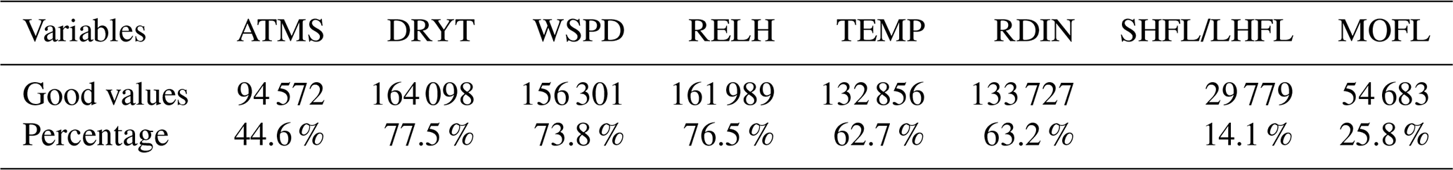
Table 4 Number of data flagged as 4 in the final flux data products for each region. In addition, the corresponding percentage of the total number of available data is displayed.

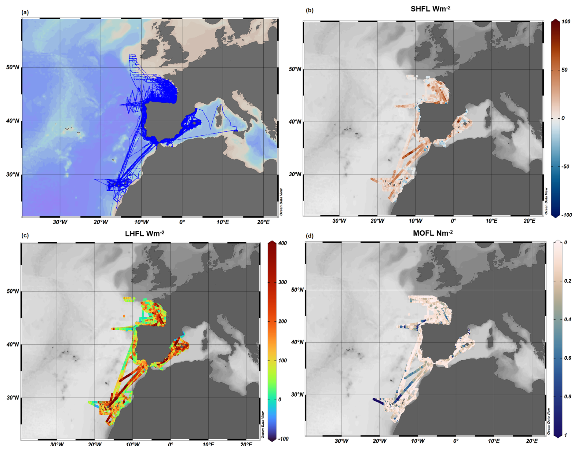
Figure 3b–d show an example of oceanographic visual products that can be represented with this data set using Ocean Data View (ODV) software (Schlitzer, 2025), where air–sea fluxes calculated are plotted throughout the vessels' trajectories at the points where they are available. These plots give a visual idea of the spatial distribution and magnitude of each variable. Differences can be noticed between basins. The Mediterranean area exhibits higher evaporation amounts in comparison with the Atlantic facade. Sensible heat characteristics are less remarkable in these areas. Nevertheless, negative values in the Alboran Sea and along the Atlantic coast in the northwest of Spain stand out. In addition, the effect of the wind stress due to the trade winds is also noticeable in the Canary region for all air–sea interaction fluxes.

Figure 3 AJ, RM, MO, and CS trajectories (a) and SHFL (b), LHFL (c), and MOFL (d) obtained during the extended period of 2011–2023. Figure obtained using ODV software (Schlitzer, 2025).

4.2 Annual cycles

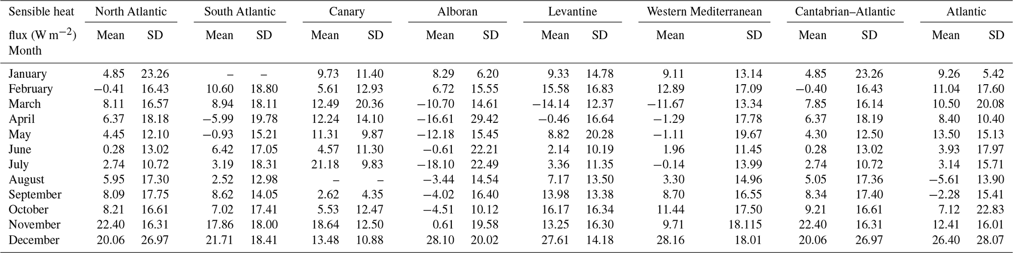
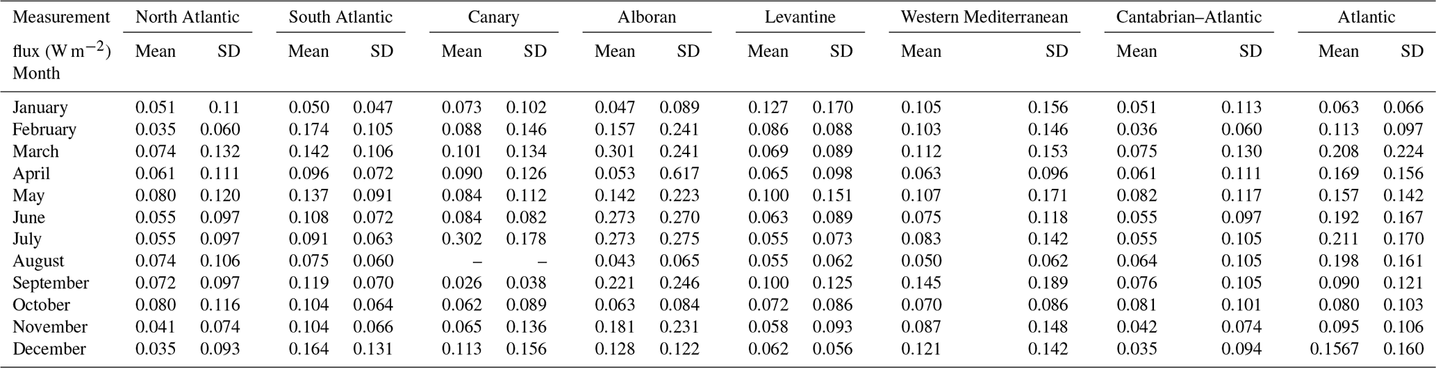
Further analysis processes can be carried out with these data sets. Annual cycles provide key information for understanding the mean behaviour and variability of a field at inter-annual frequencies. They also contribute to both validating the data and identifying key or eye-catching patterns to be analysed further. In this case, Table 5 shows the annual cycle for the sensible heat flux for each sea region considered. All regions manifest a similar behaviour, with the lowest values during the summer season (from June to August) and the highest results for November and December, showing a greater loss of heat by the ocean during winter months due to the contrast in terms of temperature between the sea surface and air. The annual mean is positive over the whole domain, with the highest quantities for the Canary (9.86 W m⁻²) and Levantine–Balearic (6.71 W m⁻²) regions, excluding the Alboran Sea, where several negative values are present and which conforms to an annual mean of −2.26 W m⁻². The special behaviour of this region, with an average annual cooling, compared to that of other basins is also detailed in the scientific literature (Vargas-Yáñez et al., 2007; Ruiz et al., 2008). Some hypotheses to be considered to explain this behaviour are the income of colder North Atlantic waters or the upwelling processes of the Poniente wind regime (Ortega et al., 2023) and the two anticyclonic gyres in this basin (Sarhan et al., 2000). The standard deviation values, despite presenting amounts even higher than the mean result, are compatible with those of other studies.

Table 5 SHFL annual cycle for each region. Shown are the mean and standard deviation (SD) for each month during the period of 2011–2023. Dashes mean no values were available due to lack of measurements.

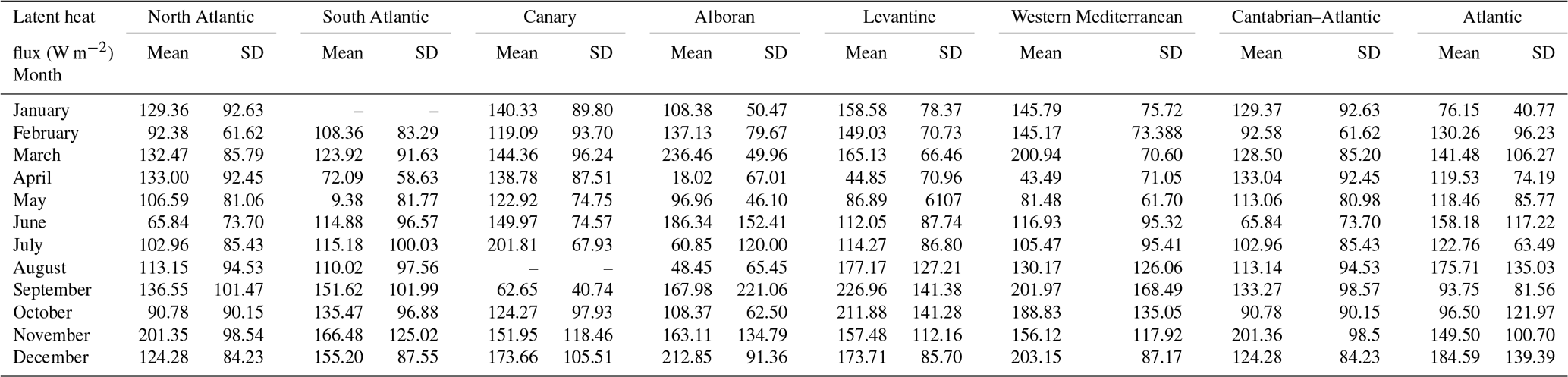
Regarding latent heat flux (Table 6), the annual cycle pattern is similar to that of the sensible heat but with greater values: lower quantities during the spring–summer transition and higher values during the winter season when wind stress is more intense. This confirms the greater loss of heat during winter months due to turbulent exchange. Higher annual mean values are found once again in the Canary (138.35 W m⁻²) and Levantine–Balearic (139.50 W m⁻²) regions. These behaviours are expected as the former is located in subtropical latitudes, commonly known to be areas with great levels of evaporation (Hartmann, 2015), whereas the latter belongs to the Mediterranean basin, where the evaporation regime is equally significant, even exceeding precipitation rates (Talley, 2011). The annual average within the Mediterranean area is slightly superior to that of the other model-based reconstructions (Yu and Weller, 2007; Ruiz et al., 2008); nonetheless, their ranges of variability are compatible. More moderate values are found within the Cantabrian and Atlantic areas, where precipitation exceeds evaporation. However, there are significant quantities that must be validated by additional studies.

Table 6 LHFL annual cycle for each region. Shown are the mean and standard deviation (SD) for each month during the period of 2011–2023. Dashes mean no values were available due to lack of measurements.

Momentum flux outcomes present expected values within the characteristic ranges of the specific location (Table 7). The annual mean values for all regions are around 0.1 N m⁻². This quantity is exceeded in several regions during the months of November and December, enabling greater turbulent exchange between the ocean and the atmosphere. This is logical due to the atmospheric baroclinicity and the intensification of the wind regimes of these months. However, annual cycles are not satisfactorily defined for all regions. The Alboran–Strait area shows higher-than-expected values during July and August, in contrast with the inter-annual wind climatology of their regional winds, namely the Levante–Poniente regime (Camacho et al., 2022). The Canary region also presents higher results during August, although this is already documented in the scientific literature (Azorin-Molina et al., 2018).

Table 7 MOFL annual cycle for each region. Shown are the mean and standard deviation (SD) for each month during the period of 2011–2023. Dashes mean no values were available due to lack of measurements.

4.3 Time series

The time series of heat and momentum fluxes are also plotted to analyse the evolution, tendencies, and gaps during the period considered. The western Mediterranean and the Cantabrian–Atlantic graphics are shown in Fig. 4 as they are the regions with more extension in this study. The data gap during the year 2020 and at the beginning of 2021, due to the difficult working context of the COVID pandemic, stands out. Uniquely, the AJ's data are available during this time frame, although with several problems in the temperature probe and the barometer which make it impossible to make a reliable calculation of the final products. These gaps are difficult to interpolate due to the high variability of the meteorological magnitudes implied in the flux calculation, creating a complicated context in which to study hypothetical tendencies or patterns, which are blurred by the intermittence of the time series. Thorough maintenance and care of the measuring equipment are fundamental in order to take advantage of the experimental measuring potential. However, several important conclusions can be drawn: the Mediterranean area exhibits greater latent heat fluxes due to the dominance of evaporation in its basin. Sensible heat is higher for the Cantabrian basin; the negative values from the Alboran Sea, aforementioned, decrease the mean value of the Mediterranean basin. Regarding momentum flux, the mean values for all of the basins are around 0.1 N m⁻², which is an expected quantity for these basins (Samuel et al., 1999; Trenberth et al., 1990), with the highest value being for the Alboran Sea, presumably due to the influence of the Levante–Poniente wind regime (Ortega et al., 2023).

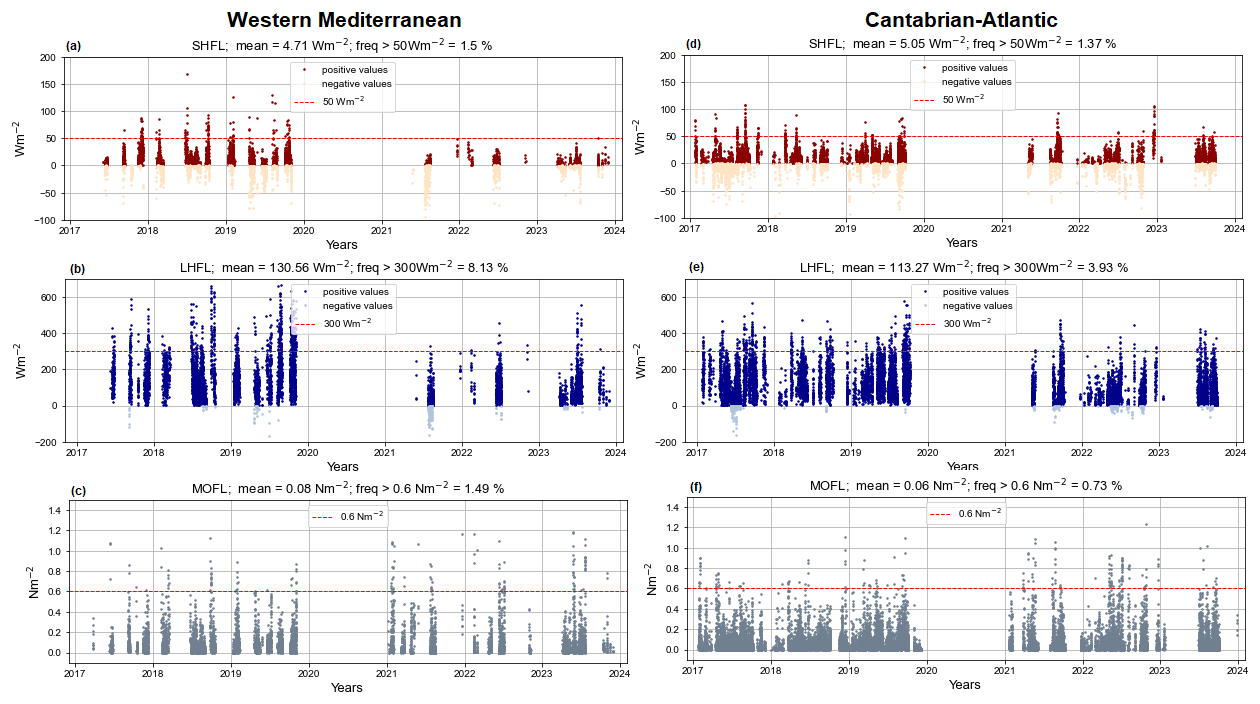
Figure 4 SHFL, LHFL, and MOFL time series (2017–2023) for the western Mediterranean (a–c) and Cantabrian–Atlantic (d–f) regions. The dashed red line denotes the thresholds of 50 W m⁻², 300 W m⁻² and 0.6 N m⁻², respectively, for each magnitude.

The levels of 50 and 300 W m⁻² for sensible and latent heat, respectively, which are considered to be significant magnitudes for both variables, are marked by dashed red lines. The regions of the planet where the greatest turbulent heat exchange between the ocean and the atmosphere occurs are the western margins of the Atlantic and Pacific oceans, in the Gulf and Kuroshio currents, respectively, where these thresholds are exceeded (Hartmann, 2015). On the other hand, the 0.6 N m⁻² threshold is defined for momentum flux based on the results of other studies in open-ocean conditions (Large and Pond, 1981). Regions with remarkable wind intensity regimes, such as the Southern Ocean, can reach values superior to 1 N m⁻² (Trenberth et al., 1990; Morrow et al., 1992) or even greater (2–8 N m⁻²) during tropical cyclones (Morrow et al., 1992). The Alboran Sea expresses one of the highest frequencies (0.76 %) of momentum flux, exceeding this threshold, while it has the lowest ratio above the 50 W m⁻² sensible heat threshold – also expected because of its negative average value. In addition, the Levantine area shows the highest frequency (8.80 %) above the 300 W m⁻² barrier. On the contrary, the Cantabrian region has the lowest ratio for this variable (3.93 %), indicating a lower evaporation rate in comparison.

Furthermore, in order to address the issue of the lack of heat and momentum flux outcomes due to the absence of a necessary variable for their calculation, the evolution of key variables that significantly influence the final products (Eqs. 4–6) can be examined separately (Fig. 5). The temperature difference is directly proportional to the sensible heat flux, and it allows us to define the sign of this flux and to assess whether it implies a positive or negative heat contribution to ocean warming. Additionally, wind speed is proportional to all three air–sea interaction fluxes, and so its behaviour is crucial for inferring the magnitude of these products. Besides this, relative humidity is essential for determining the specific humidity of the air and, thus, the moisture difference compared to the ocean, which is proportional to latent heat flux. The higher the relative humidity, the less likely it is that water evaporation from the ocean will occur as the environment reaches saturation; in consequence, this potential energy remains stored in the ocean rather than being transferred to the atmosphere.

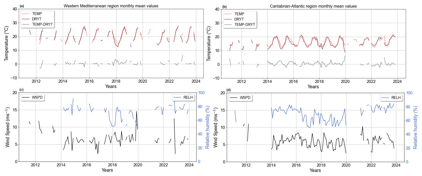
Figure 5 Time series of monthly average variables: sea temperature (orange), air temperature (red), and their difference in grey (a, b) and wind speed (c, d) for the western Mediterranean (a, c) and Cantabrian–Atlantic regions (b, d).

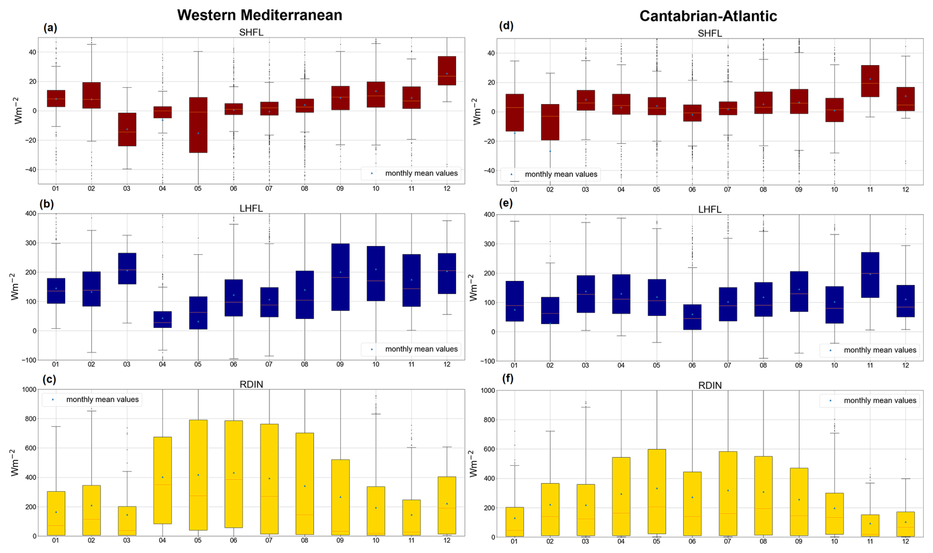
Figure 6 Annual cycle of SHFL (a), LHFL (b), and total incident radiation (RDIN, c) during the period of 2011–2023 for the western Mediterranean (a–c) and Cantabrian–Atlantic (d–f) areas.

4.4 Heat budget

One additional application of the study of air–sea interaction fluxes is to obtain the net heat storage balance. The ocean heat budget is determined by both radiative (net shortwave and longwave radiation) and convective components. Sensible and latent heats account for the convective contribution, whereas the incident radiation is provided by the RDIN variable (Fig. 6c and f) measured by the meteorological measuring equipment. It accounts for the solar (shortwave) and atmospheric (longwave) radiation. The longwave emission by the ocean can be determined by the Stefan–Boltzmann law with the specific determination of the emissivity constant for ocean water (Fung et al., 1984). Beyond this, given that the ocean is not a fixed water mass, the advective-heat term might have an important magnitude to be considered in the heat balance (Anderson, 1952). The Atlantic Meridional Overturning Circulation (AMOC) accounts for most of the northward transport of heat by the mid-latitude Northern Hemisphere (Talley, 2003). It reaches its peak heat transport around 26° N, where, consequently, the RAPID Climate Change Programme was established in 2004 to provide direct observational measurements of its flow and transport (Johns et al., 2011). Thus, this certainly has an important impact on the heat storage balance of the Canary region, which is close to this latitude, not to mention the impact on the rest of the Atlantic marine regions considered in this study. Regarding the Mediterranean Sea, mooring-based observations have established the net heat transport from the Atlantic through the Strait of Gibraltar to be 5.2 W m⁻² (Macdonald et al., 1994). Other authors have determined this flux to be between 8.5 W m⁻² (Bethoux, 1979) and 5 W m⁻² (Bunker et al., 1982) based on measurements of the net water inflow and its temperature.

Figure 6 shows the annual cycles of the heat convective fluxes (Fig. 6a, d, b, and e) and the incident radiation (Fig. 6c and f) for two example regions, the western Mediterranean and the Cantabrian–Atlantic areas. Sensible and latent fluxes reach their minimum strength during the spring–summer transition, whereas they are more prominent during the colder seasons. On the contrary, the incident radiation presents a reverse pattern. During summer, less heat is lost by turbulent processes, and more is acquired by radiation, increasing the total heat budget. On the other hand, in winter, when there is a positive and marked contrast between the sea and air temperature, sufficient wind stress to trigger the convective fluxes, and less incident radiation, the ocean experiences a decrease in its heat storage.

Incident radiation is greater for the Mediterranean region than for the Cantabrian due to the differences in terms of their geographical location and cloud cover. However, in comparison to other studies in the former area (Lozano et al., 2023), monthly mean radiation values might present some deficits, which contribute to underestimations of the heat income stored in the ocean, altering the total heat balance. Further comparisons and validation procedures must be done regarding incident radiation in order to obtain fairly reliable heat storage outcomes.

Sánchez-Lorente and Tel (2024a)Sánchez-Lorente and Tel (2024b)Sánchez-Lorente and Tel (2024c)Sánchez-Lorente and Tel (2024d)

Table 8 DOIs for each data set for each research vessel, publicly available at SEANOE.

5 Data availability

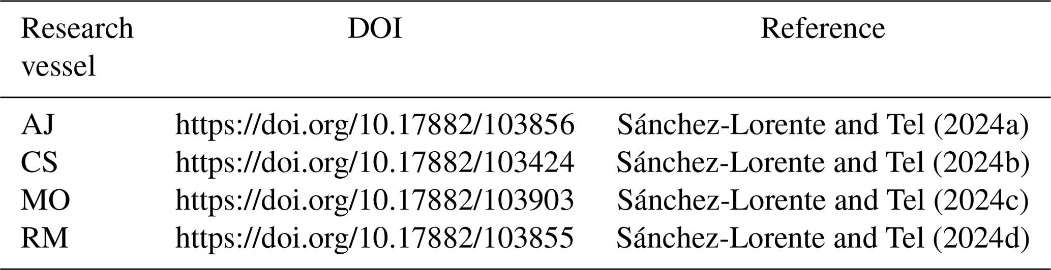
All data are publicly available at the SEANOE (SEA scieNtific Open data Edition) data citing and publishing service of SeaDataNet (https://www.seadatanet.org/Software/SEANOE, last access: 19 October 2025). The data have been classified by vessel and month within MEDAR/MedAtlas format. The data set DOIs for each research vessel are shown in Table 8.

6 Conclusion

This paper presents the air–sea interaction heat and momentum flux data obtained through meteorological and TSG observational measurements collected during the activities of the AJ, RM, MO, and CS research vessels between 2011 and 2023. The calculation methodology of the sensible, latent, and momentum fluxes is the bulk aerodynamic approximation (Large and Yeager, 2009), which relies on the gradient of temperature, specific humidity, and horizontal wind between the air and the sea surface. The vessels' trajectories cover a large part of the Spanish waters and adjacent seas, waters showing notorious heterogeneity due to the different latitudinal extent, as well as the distribution of the surrounding continental platforms. Thus, this heterogeneous character encourages the subdivision into different regions as proposed in this study.

The hourly sample frequency of the data allows us to establish a significant data coverage. This amount of information is revised and checked by quality control procedures so as to obtain reliable and operable data products. The atmospheric pressure is the variable with fewer good-value (flagged as 1) results. It presents a percentage of valid values of 44.6 % for flux calculation with respect to the total sampling (especially due to the absence of this measurement from 2013 to 2016), accounting for a total of 94572 good values that are still worth preserving. Other atmospheric variables present better percentages. Relative humidity and wind speed show considerable notorious percentages, 76.5 % and 73.8 %, respectively, despite technical issues such as relative humidity values below 0 % and above 100 % or slightly disproportionate wind velocity, both within the CS records. On the other hand, air temperature surpasses these numbers of good values, with a percentage of 77.5 % in spite of the occasional high values recorded by AJ, specifically during the 2018 and 2019 winter seasons. To all of the concrete technical issues, the difficult context of the COVID pandemic is added. In conjunction, these all create gaps in the final flux products. This complicates characterising tendencies; however, behaviours or biases can still be inferred. Thus, it is important to highlight the need for thorough and rigorous care and maintenance of the vessels' measuring equipment so as to profit from the considerable investment in the much-needed experimental recording.

Despite the mentioned technical difficulties, the values of the three fluxes are within the expected ranges for each region and season. Lower values are found during the summer season, whereas higher ones are present in the winter months. Sensible flux presents higher values in the Canary region, with an annual mean of 9.86 W m⁻²; on the contrary, the Alboran–Strait area shows a negative average of −2.26 W m⁻², compatible with other studies (Vargas-Yáñez et al., 2007; Ruiz et al., 2008). Along the same line, latent heat flux presents higher values in the Canary and the Levantine–Balearic regions (annual means of 139.01 and 139.50 Wm⁻², respectively), although it also shows slightly superior values compared to other model reconstructions (Yu and Weller, 2007; Ruiz et al., 2008). Momentum flux exhibits averages of around 0.1 Nm⁻² for all regions, with larger values within the Alboran–Strait region (annual mean of 0.12 Nm⁻²), influenced by the regional Levante–Poniente wind regime in this area (Camacho et al., 2022). Furthermore, this data set brings about the opportunity to study the heat budget storage of the ocean. The total incident radiation is added to the air–sea heat fluxes. The longwave emission from the sea can be obtained using the sea temperature and the Stefan–Boltzmann law with the correct determination of the emissivity for ocean water (Fung et al., 1984). The total incident radiation exhibits some deficits in different areas, which, added to the slightly high values of the heat fluxes, might establish negative biases to consider within the heat storage balance.

Experimental records, despite presenting several drawbacks such as data-sampling density, incomplete data series, or technical recording issues, are needed for the calibration and validation of other model- or satellite-based products that enable a better global coverage and data homogenisation despite relying necessarily on observations. Thus, attention must be paid to this direct information, especially within the ocean. Here, the meteorological and sea surface information, as well as the final flux products of the four vessels up to 2023, are presented; nevertheless, AJ, RM, and MO are still active research vessels whose recordings can be used further for the same purposes as in this paper, not to mention other research ships of the IEO.