the Creative Commons Attribution 4.0 License.
the Creative Commons Attribution 4.0 License.
 | 18 Aug 2025
A new-generation internal tide model based on 30 years of satellite sea surface height measurements: multiwave decomposition and isolated beams
An internal tide model, ZHAO30yr, is developed using 30 years of satellite altimetry sea surface height (SSH) measurements from 1993 to 2022 by a recently improved mapping technique that consists of two rounds of plane wave analysis with a spatial bandpass filter in between. Prerequisite wavelengths are calculated using climatological annual mean hydrographic profiles in the World Ocean Atlas 2018. ZHAO30yr only extracts the 30-year phase-locked internal tide component, lacking the incoherent component caused by the time-varying ocean environment. The model contains 12 internal tide constituents: eight mode-1 constituents (M2, S2, N2, K2, K1, O1, P1, and Q1) and four mode-2 constituents (M2, S2, K1, and O1). Model errors are estimated to be lower than 1 mm in the SSH amplitude on global average, thanks to the long data record and improved mapping technique. The model is evaluated by making internal tide correction to independent altimetry data for 2023. A total of 10 constituents (but for K2 and Q1) can reduce variance on global average. K2 and Q1 can only cause variance reductions in their source regions. The model decomposes the multiconstituent, multimodal, multidirectional internal tide field into a series of simple plane waves at each grid point. The decomposition reveals unprecedented features previously masked by multiwave interference. The model divides each internal tide constituent into components by propagation direction. The directionally decomposed components show numerous long-range internal tidal beams associated with notable topographic features. The semidiurnal internal tidal beams off the Amazon shelf and the diurnal internal tidal beams in the Arabian Sea are examined in detail. ZHAO30yr is available at https://doi.org/10.6084/m9.figshare.28078523 (Zhao, 2024b). Model errors are available at https://doi.org/10.6084/m9.figshare.28559978.v3 (Zhao, 2025).
- Article
(29222 KB) - Full-text XML
-
Supplement
(11588 KB) - BibTeX
- EndNote


Internal tides (internal gravity waves at tidal frequencies) are inherent wave motions in the interior of the stratified ocean (Wunsch, 1975; Munk and Wunsch, 1998; Garrett and Kunze, 2007). Internal tides are mainly generated by barotropic tidal currents flowing over variable topography (Egbert and Ray, 2000; Smith and Young, 2002; Nycander, 2005). They propagate over hundreds to thousands of kilometers and redistribute the converted tidal energy in the open ocean (Ray and Mitchum, 1996; Alford, 2003; Zhao, 2014; MacKinnon et al., 2017). Internal tides gradually lose their coherence (phase locking) with the barotropic tidal forcing in long-range propagation through the time-varying ocean. Fortunately, a fraction of internal tides remain coherent and thus detectable by multiyear time series from field moorings, acoustic thermometry, and satellite altimetry (Ray and Mitchum, 1996; Alford, 2003; Dushaw, 2022). In recent years, internal tides have drawn great research interest because they play an important role in various ocean processes including tracer transport, acoustic transmission, coral bleaching, primary productivity, and ocean mixing (Jayne and St. Laurent, 2001; Colosi and Munk, 2006; Tuerena et al., 2019; Whalen et al., 2020; Zhang et al., 2021; Dushaw, 2022; Jacobsen et al., 2023; Guan et al., 2024). In particular, internal tides can be used for monitoring global ocean changes, in that their speed changes in long-range propagation contain important information on ocean stratification (Zhao, 2016). Internal tides may be unwanted noise in some research and should thus be accurately corrected (Morrow et al., 2019; Yadidya et al., 2024). In the past decade, a few empirical internal tide models have been constructed from satellite altimetry (Ray and Zaron, 2016; Zhao et al., 2016; Zaron, 2019; Zhao, 2023b; Zaron and Elipot, 2024). On the other hand, internal tide models have been developed by numerical simulations driven by atmospheric forcing and tidal potential (Simmons et al., 2004; Müller et al., 2012; Shriver et al., 2012; Buijsman et al., 2017; Arbic et al., 2018; Li and von Storch, 2020; Arbic, 2022). Internal tide models can also be developed using semi-analytical methods (Nycander, 2005; Pollmann and Nycander, 2023; Geoffroy et al., 2025). In this paper, I will present a new internal tide model developed using 30 years of satellite altimetry sea surface height (SSH) measurements from 1993 to 2022.
Satellite altimetry observes internal tides via their small SSH fluctuations and thus provides a unique tool for mapping internal tides on a global scale. However, their weak SSH signals are usually overwhelmed by leaked mesoscale signals (mesoscale contamination) because the internal tide field is spatially and temporally under-sampled by satellite altimetry. Previous studies mainly focused on the first baroclinic modes of M2, S2, K1, and O1 constituents (Carrere et al., 2021). Previous internal tide models usually contain considerable errors, but none provide error estimates. The oceanographic community needs accurate and complete internal tide models in various research such as quantifying coherent and incoherent internal tides, internal-tide-induced ocean mixing, and internal tide–eddy interactions. These questions require better knowledge of the global internal tide field. Previous advances are due mainly to the accumulation of multiyear multimission altimetry data because a longer data record may lead to lower errors. Some recent altimetry missions (phases) are operated along nonrepeat tracks (Zhao, 2022a). For example, CryoSat-2 has a long repeat period of 369 d and samples the ocean along 10 668 ground tracks (Wingham et al., 2006). Haiyang-2A has 386 ground tracks in its exact-repeat phase and 4630 ground tracks in its geodetic phase. The nonrepeat ground tracks greatly improve spatial resolution because the denser ground tracks allow us to map internal tides in smaller fitting windows (Zhao, 2022a).
I have been improving my mapping technique over the past decade to construct better and better internal tide models (Zhao, 2021, 2022a, b, 2023b). My core technique is plane wave analysis that extracts waves in different horizontal directions. My mapping technique has been adapted to nonrepeat altimetry missions. Previous pointwise harmonic analysis cannot extract internal tides from nonrepeat altimetry missions because the SSH time series at any given point is too short to extract reliable internal tides. The pointwise harmonic analysis employed in Zhao et al. (2016) has been replaced with plane wave analysis, and thus my improved mapping procedure uses plane wave analysis twice. The along-track one-dimensional bandpass filter in Zhao et al. (2016) has been replaced with a spatial two-dimensional bandpass filter to extract internal tides having large angles with ground tracks. Thus, my new mapping technique consists of two rounds of plane wave analysis with a spatial bandpass filter in between (Zhao, 2022a, b). It maps the internal tide field in three rounds of temporal and spatial filtering, taking advantage of preknown tidal periods and wavelengths of the target internal tides.
This paper reports a new internal tide model developed by applying my improved mapping technique to 30 years of satellite altimetry data from 1993 to 2022. The new internal tide model is called ZHAO30yr. The model decomposes the internal tide field and thus reveals numerous long-range internal tidal beams. Note that it is important to resolve the multiwave interference pattern to correctly interpret in situ and satellite observations (Rainville et al., 2010). However, all previous internal tide models give the multiwave summed internal tide fields and do not resolve internal tidal beams (Carrere et al., 2021). As shown in this paper, the decomposed internal tidal beams contain key information on their generation, propagation, and dissipation.
ZHAO30yr has the following outstanding features.
-
The model provides model errors that are estimated by background internal tides (Zhao, 2023b). The combination of a long data record and improved mapping technique reduces model errors down to lower than 1 mm on global average; therefore, I can extract the much weaker minor and mode-2 internal tide constituents.
-
The model contains 12 internal tide constituents: eight mode-1 constituents (M2, S2, N2, K2, K1, O1, P1, and Q1) and four mode-2 constituents (M2, S2, K1, and O1). It contains more constituents than any previous empirical internal tide model mentioned in Carrere et al. (2021, Table 1).
-
The model resolves each of the 12 internal tide constituents by five-wave decomposition. The global, multiconstituent, multimodal, multidirectional internal tidal field is thus decomposed into 60 simple plane waves at each grid point. The decomposition reveals many new features that were previously masked by multiwave interference.
-
The model contains directionally decomposed components, which reveal numerous well-defined long-range internal tidal beams associated with notable topographic features. The beams are characterized by larger amplitudes, linear increasing phases, and across-beam co-phase lines.
The remainder of this paper is arranged as follows. Section 2 briefly describes the satellite altimetry data and ocean stratification data used in this study. Section 3 gives a detailed description of my mapping procedure and key mapping parameters. Section 4 estimates model errors and evaluates the model using independent altimetry data. Section 5 examines the decomposed components and shows numerous internal tidal beams. Section 6 examines in detail the internal tidal beams off the Amazon shelf and in the Arabian Sea. Section 7 is a summary. Section 9 contains model limitations and perspectives.
2.1 Satellite altimetry data
The internal tide model is developed using 30 years of satellite altimetry SSH measurements from 1993 to 2022 (Fig. 1, red box). The data are pre-processed and distributed by the Copernicus Marine Service (https://doi.org/10.48670/moi-00146, CMS2025a, 2025). The SSH measurements are made by 15 nadir altimetry missions. The merged data record is about 120 years long. The multisatellite altimetry data have higher spatial resolution because the SSH measurements are along both exact-repeat and nonrepeat tracks (Zhao, 2022a, b). The data have been pre-processed for standard geophysical corrections including atmospheric effects, surface wave bias, geophysical effects, barotropic tide, pole tide, solid Earth tide, and loading tide (Taburet et al., 2019). The mean sea surface model used in this satellite altimetry product is CNES-CLS15 (Pujol et al., 2018). The SSH measurements from seven nadir altimetry missions in 2023 are reserved for model evaluation (Fig. 1, blue box).
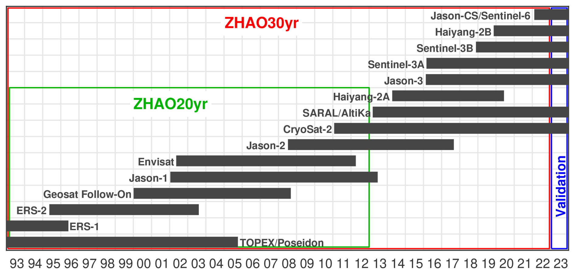
Figure 1Satellite altimetry data. ZHAO20yr and ZHAO30yr are developed using 20 (1993–2012) and 30 (1993–2022) years of altimetry data, respectively. Altimetry data for 2023 are reserved for model evaluation.
The SSH signals of mesoscale eddies are about 1 order of magnitude greater than the internal tide signals. Directly mapping internal tides without mesoscale correction would lead to large model errors (Ray and Zaron, 2016; Zhao et al., 2016). Mesoscale correction was brought up by Ray and Byrne (2010) and has been employed in a number of studies (Ray and Zaron, 2016; Zaron, 2019; Zhao, 2022b). In this study, prior mesoscale correction is made using the two-dimensional (2D) gridded SSH fields distributed by the Copernicus Marine Service (https://doi.org/10.48670/moi-00148, CMS2025b, 2025). The fields are gridded daily in time and 0.25° by 0.25° in the horizontal. Prior to mesoscale correction, the gridded SSH fields are 2D low-pass-filtered to remove leaked internal tide signals (Ray and Zaron, 2016; Zaron, 2017). Cutoff wavelengths of 200 km (300 km) are used for data sets prepared for mapping semidiurnal (diurnal) internal tides. The mesoscale signals are then interpolated and removed from the along-track SSH data (Ray and Byrne, 2010; Ray and Zaron, 2016; Zaron, 2019; Zhao, 2022b). Note that mesoscale correction is affected by the chosen cutoff parameters (Zaron and Ray, 2018). Mesoscale correction is an indispensable step to suppress mesoscale contamination, although it cannot perfectly remove mesoscale signals.
2.2 Internal tide wavelengths
My mapping technique requires tidal periods and wavelengths of the target internal tides. The periods (frequencies) of internal tides are astronomical constants that have been well documented in classic textbooks (e.g., Pugh and Woodworth, 2014) and software packages (e.g., Egbert and Erofeeva, 2002; Pawlowicz et al., 2002). Table 1 gives the tidal periods of the eight principal constituents studied in this paper (M2, S2, K1, O1, N2, K2, P1, and Q1). There are two pairs of internal tide constituents that are separated by two cycles per year (cpy). One pair is K1 (23.9345 h) and P1 (24.0659 h). The other pair is S2 (12 h) and K2 (11.9672 h). For the barotropic tide, at least a 6-month hourly data record is needed to separate each pair. In this study, I show that 30 years of altimetry data with irregular sampling rates can separate both constituent pairs.
The internal tide wavelengths are calculated using the climatological annual mean hydrographic profiles in the World Ocean Atlas 2018 (WOA18) provided by the NOAA National Centers for Environmental Information (https://www.nodc.noaa.gov/OC5/woa18/, last access: 30 July 2025). The WOA18 hydrography is on a spatial grid of 0.25° by 0.25°. For a given ocean depth and stratification profile, the vertical structures and eigenvalue speeds of discrete baroclinic modes are obtained by solving the Sturm–Liouville orthogonal problem (Gill, 1982; Kelly, 2016),
subject to free-surface (not rigid-lid surface) and rigid-bottom boundary conditions, where N(z) is the buoyancy frequency profile, Φ(z) and cn are the eigenvector and eigenvalue, and the subscript n is the modal number. With Earth's rotation, wavelength λn can be calculated from the eigenvalue speed cn following , where ω and f (≡ 2Ωsin(latitude), where Ω is Earth's rotation rate) are the tidal and inertial frequencies, respectively. The resulting global wavelengths for the semidiurnal and diurnal internal tide constituents are shown in Figs. S1 and S2 in the Supplement, respectively. It is well known that wavelengths are a function of location, in particular latitude. Table 1 gives their global mean wavelengths (within ±60° for semidiurnal constituents and ±26.5° for diurnal constituents). For the eight mode-1 constituents, the mean wavelengths range from 129.5 km for S2 to 404.5 km for Q1. The mode-2 K1 and O1 internal tides have mean wavelengths of 163.8 and 191.2 km, respectively, longer than mode-1 semidiurnal constituents. The mode-2 M2 and S2 constituents have wavelengths shorter than 80 km. Mode-1 K1 and P1 have close wavelengths (294.1 and 294.3 km); therefore, it is challenging to separate these two constituents. This study shows that one can extract reasonable K1 and P1 internal tides using 30 years of altimetry data.
Table 1Properties and empirical mapping parameters of the 12 internal tide constituents.
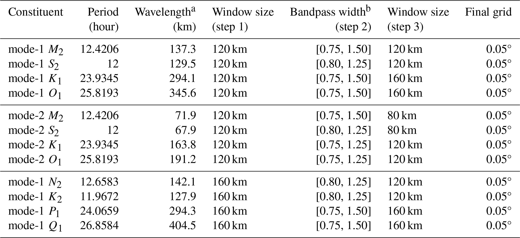
a Global mean wavelength within ±60° (semidiurnal) and ±26.5° (diurnal).
b Bandpass width multiplied by the local wavenumber K(long, lat) yields bandpass cutoff wavenumbers.
My recently improved mapping procedure consists of two rounds of plane wave analysis with a spatial bandpass filter in between (Zhao, 2022a, b). An example of the three-step mapping procedure can be found in Zhao (2022a, Fig. 3). In the first step, one target internal tide constituent is mapped by plane wave analysis. At each grid point, five internal tidal waves of arbitrary propagation directions are determined (Sect. 3.1). The vector sum of these five waves gives the internal tide solution. This step yields a global internal tide field on a regular latitude–longitude grid from the sparse satellite along-track SSH data. In the second step, the regularly gridded internal tide field is cleaned by spatial bandpass filtering (Sect. 3.2). The target internal tide field is converted to the 2D wavenumber spectrum by Fourier transform, and the spectrum is truncated by bandpass width times the local wave number (Zhao, 2022b). Empirical bandpass widths are given in Table 1. In the third step, plane wave analysis is used again to decompose the filtered internal tide field into five internal waves at each grid point. The second-round plane wave analysis is the same as the first-round plane wave analysis, but the input is the filtered internal tide field in the second step. In the end, the resulting five waves are saved with their respective amplitudes, phases, and directions. The five-wave decomposition makes it possible to separate internal tides in different propagation directions.
3.1 Plane wave analysis
My core technique for mapping internal tides from satellite altimetry data is plane wave analysis developed in a series of previous studies (Zhao and Alford, 2009; Zhao, 2014; Zhao et al., 2016; Zhao, 2022a). Plane wave analysis evolves from the two-dimensional plane wave fit method (Ray and Cartwright, 2001), but plane wave analysis extracts multiple waves in different propagation directions and thus resolves multiwave interference (Zhao and Alford, 2009). Plane wave analysis determines internal tides using SSH measurements in a square fitting window. At each grid point, the internal tide solution is mapped using along-track altimetry data in a fitting window centered at the grid point. Each fitting window thus contains a large number of independent SSH data. One target internal tidal wave has three parameters to be determined: amplitude A, phase ϕ, and propagation direction θ. There are multiple waves of arbitrary propagation directions at one site; therefore, five target internal tidal waves are fitted following
where x and y are the east and north Cartesian coordinates, t is time, T and λ are the period and wavelength of the target wave, and f(t) and u(t) are the nodal factor and phase for the 18.6-year cycle, respectively. The lunar nodal cycle is taken into account (Pugh and Woodworth, 2014) because the altimetry data are longer than 18.6 years. An iterative algorithm has been developed to extract five internal tidal waves in different propagation directions. Examples can be found in Zhao (2014, Fig. 3) and Zhao et al. (2016, Fig. 2). In each step, the amplitude A, phase ϕ, and propagation direction θ of one target internal tidal wave are determined using SSH data in one given fitting window by least-squares fit. To do that, the amplitude and phase of one plane wave are determined in each compass direction (angular increment is 1°). When the resultant amplitudes are plotted as a function of direction in polar coordinates, an internal tidal wave appears to be a lobe. The amplitude and direction of the target wave are thus determined from the largest lobe. After that, the signal of the determined wave is predicted and removed from the original SSH data. This step is repeated five times to determine five target internal tidal waves. In the end, each wave is refitted with the other four waves temporally removed to reduce the wave–wave interference. The five internal tidal waves are usually sorted with decreasing amplitudes, and their vector sum gives the internal tide solution at the grid point.
3.2 Spatial bandpass filtering
Using the spatially regular internal tide field obtained by plane wave analysis, the internal tide field can be converted to a 2D wavenumber spectrum by Fourier transform in overlapping 850 by 850 km windows. I have tested different spatial windows and found that the filtering is insensitive to the window size. The 2D wavenumber spectrum shows that the variance is mainly around the theoretical wavenumber. The variance falling outside the theoretical wavenumber range is considered noise. Thus, the 2D wavenumber spectrum is truncated and converted back to the internal tide field by inverse Fourier transform. The width of the bandpass filter (e.g., cutoff wave numbers) is empirically determined (Table 1). It reflects the spectral peaks of the target internal tide constituent determined by the length of the data record. The bandpass width is affected by the fitting window employed in plane wave analysis and noise level. To reduce the ringing effect of artificial wiggles occurs in the boundary layer, I throw away the filtered values in the outer 100 km boundary layer and only keep values in the inner region. An example of the spatial 2D bandpass filter can be found in Fig. 4 of Zhao et al. (2019).
3.3 Special issues
There are some issues in the model development that require special attention. First, Sun-synchronous altimetry missions, including ERS-1/2, Envisat, and Haiyang-2A/2B, have an aliasing issue with the S2 tide. Previous studies have usually mapped S2 internal tides excluding Sun-synchronous missions (Zhao, 2018; Zaron, 2019). It is a surprise that Ubelmann et al. (2022) can map S2 internal tides including data from Sun-synchronous missions. In this study, mode-1 and mode-2 S2 internal tides are mapped using all altimetry missions including Sun-synchronous missions (Fig. 1, red box). The result shows that my new S2 internal tide model has a higher spatial resolution and lower model errors. It is a significant improvement over my previous S2 internal tide model (Sect. 4.3). There are three likely reasons why Sun-synchronous missions do not ruin the mapping of S2 internal tides. (1) My mapping procedure extracts internal tides not only by their frequencies in time but also by their wavelengths in space. Measurements by Sun-synchronous missions still provide useful spatial information on S2 internal tides. (2) The 30-year-long data record itself can significantly reduce model errors. (3) A large fraction of the data is from non-Sun-synchronous missions, which greatly reduces model errors. Additionally, the nontidal signals caused by solar radiance have longer spatial scales and can be reduced by spatial bandpass filtering.
Second, care is needed to separate two pairs of internal tide constituents. The first pair contains mode-1 K1 and P1 with tidal periods of 23.9345 and 24.0659 h, respectively. The second pair contains mode-1 S2 and K2 with tidal periods of 12 and 11.9672 h, respectively. To separate K1 and P1, mode-1 K1 internal tides are firstly constructed. Then P1 internal tides are mapped using the temporally K1-corrected altimetry data (e.g., predict and subtract K1 internal tides from the original data). In the end, mode-1 and mode-2 K1 internal tides are re-mapped using the P1-corrected altimetry data. Likewise, S2 and K2 can be separated following the same procedure. The results show that this method can suppress cross-talk and better separate the two constituent pairs (Sect. 4).
Third, the larger mode-1 constituents may affect the smaller mode-2 constituents. Both mode-1 and mode-2 constituents are mapped for M2, S2, K1, and O1. For each constituent, modes 1 and 2 have the same tidal period, but the mode-1 wavelengths are about twice the mode-2 wavelengths (Table 1). For each case, the mode-1 constituent may affect the mode-2 constituent, but the mode-2 constituent does not affect the mode-1 constituent. Assuming the mode-1 and mode-2 internal tide amplitudes are 15 and 5 mm, respectively, they each leak 10 % of their amplitude to the other. One can see that mode 2 leaks to mode 1 by 0.5 mm (5 mm × 10 %), which is only 3.3 % of the mode-1 amplitude. However, mode 1 leaks to mode 2 by 1.5 mm (15 mm × 10 %), which is 30 % of the mode-2 amplitude. In this study, the mode-1 constituent is firstly mapped and removed from the original data. Then the mode-2 constituent is mapped using the corrected data. Comparisons show that this measure is indispensable to extract reliable mode-2 internal tide constituents.
3.4 Mapping parameters
I extract 12 internal tide constituents from the 30 years of satellite altimetry data one by one following the same three-step mapping procedure. They are eight mode-1 constituents (M2, S2, N2, K2, K1, O1, P1, and Q1) and four mode-2 constituents (M2, S2, K1, and O1). Table 1 lists the 12 internal tide constituents and their key empirical mapping parameters. In this study, semidiurnal internal tide constituents are mapped from 60° S to 60° N and diurnal constituents from 30° S to 30° N. In the first round of plane wave analysis, a fitting window of 120 km is used for major constituents (M2, S2, K1, and O1) and 160 km for minor constituents (N2, K2, P1, and Q1). In the second round of plane wave analysis, a fitting window of 160 km is used for diurnal constituents, 120 km for mode-1 semidiurnal constituents, and 80 km for mode-2 M2 and S2 constituents. In the spatial bandpass filtering, [0.75, 1.50] is used for diurnal constituents and M2 constituents, and [0.80, 1.25] is used for other semidiurnal constituents. All constituents are finally interpolated onto a spatial grid of 0.05° by 0.05°. These mapping parameters are empirically chosen after testing several reasonable choices. My previous studies show that these mapping parameters will not affect the results much on a global scale (Zhao, 2022a, b); however, these parameters can be optimized region by region and constituent by constituent. Figure S3 shows the resulting 12 internal tide constituents. Internal tides with amplitudes lower than 1 mm are shown in light blue. The regions with large model errors due to mesoscale contamination are indicated by black contours. The results show that mode-1 M2 and K1 internal tides have the largest amplitudes, greater than 25 mm, while mode-1 K2 and Q1 internal tides have the lowest amplitudes, lower than 3 mm.
3.5 Multiwave decomposition
The global internal tide field is a superposition of multiconstituent, multimodal, multidirectional internal waves. The multiwave superposition leads to complicated spatial interference and makes it difficult to detect individual internal tidal waves and track their generation, propagation, and dissipation. In the new model, the internal tide field is decomposed into a series of simple plane waves. In frequency, eight principal internal tide constituents are extracted (M2, S2, N2, K2, K1, O1, P1, and Q1). In the vertical direction, the two lowest baroclinic modes are extracted for the four major constituents (M2, S2, K1, and O1). In the horizontal direction, each internal tide constituent is decomposed into five plane waves with empirically determined directions at each grid point. All together, 60 simple plane waves are determined at each grid point. The 12 internal tide constituents and their five wave components are shown in Figs. S4–S15.
For each constituent, the five-wave summed field shows obvious interference features such as half-wavelength fluctuations in amplitude and phase. In contrast, the five-wave resolved components are not affected much by multiwave interference. Therefore, the decomposed results reveal a lot of new features that were previously masked by multiwave interference. In particular, the first wave components (panels b in Figs. S4–S15) show the largest waves at each grid point. They have relatively larger and smoother amplitudes so that individual long-range internal tidal beams can be clearly identified. Around the Hawaiian Ridge, there are outgoing internal tidal beams in all 12 internal tide constituents. Because the Hawaiian Ridge is generally in the west–east direction, the internal tide radiation is dominantly southward and northward. Around the south–north-aligned Izu–Bonin–Mariana Arc, westward and eastward internal tidal beams exist. In the Madagascar–Mascarene region, there are outgoing internal tidal beams in all directions. However, internal tidal beams shown in Figs. S4–S15 may mix internal tidal waves from different generation sites. In this study, I show that isolated internal tidal beams should be examined using the directionally decomposed components (Sect. 5).
4.1 Model errors
Model errors (Zhao, 2025) are estimated using background internal tides following Zhao (2023a, b). Background internal tides are extracted from the same altimetry data following the same procedure but using tidal periods slightly different from the eight principal constituents. In other words, model errors are indicated by internal tide signals where internal tides do not exist. In principle, model errors are determined by the given altimetry data and the mapping technique used to extract internal tides. Background internal tides do not vary much over the narrow semidiurnal or diurnal frequency bands (Zhao, 2023b). This study estimates errors in semidiurnal internal tides using 12.3373 h (M2 minus 5 min) and in diurnal internal tides using 23.8511 h (K1 minus 5 min). Both mode-1 and mode-2 internal tide errors are estimated for the semidiurnal and diurnal constituents. The resulting model errors are shown in Fig. 2. In regions of extremely high mesoscale eddies, the semidiurnal errors are dominantly larger than 1 mm due to mesoscale contamination (mesoscale correction in Sect. 2 is not enough). These regions include the Kuroshio extension region, the Gulf Stream, the East Australian Current, the Agulhas Current, the Brazil Current, the Leeuwin Current, the loop current in the Gulf of Mexico, and the Antarctic Circumpolar Current. These regions are highlighted by black contours following Zhao et al. (2016). Fortunately, in most of the global ocean, model errors are very low (Fig. 2, blue patches). On global average, the model errors in all constituents are lower than 1 mm. The low model errors allow us to map the much weaker mode-2 constituents and minor constituents.
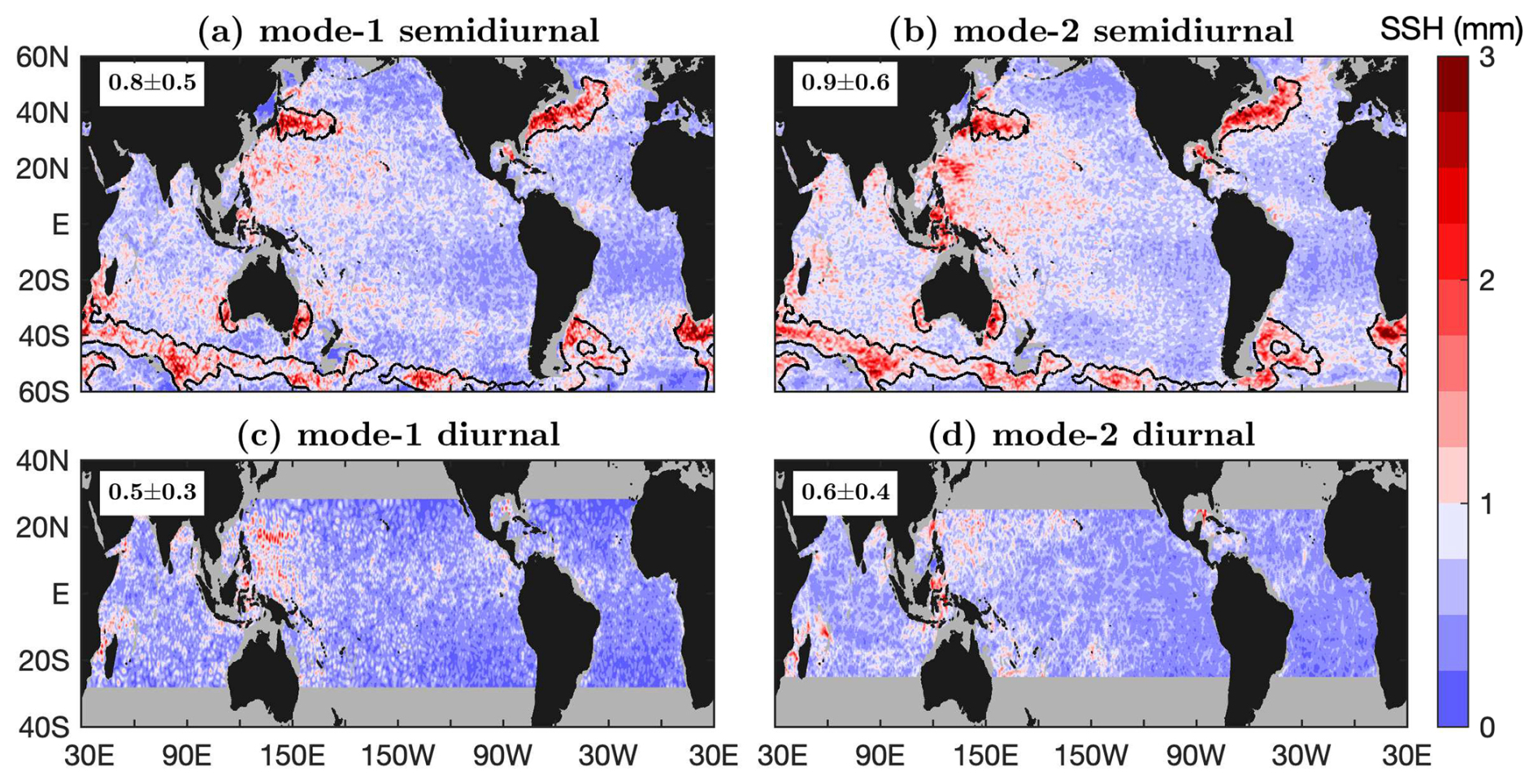
Figure 2Model errors. For each constituent, the global mean and 1 standard deviation are given in the upper left corner. Black contours indicate regions of large model errors due to mesoscale contamination.
4.2 Model evaluation
The new internal tide model is evaluated using independent nadir-looking altimetry data for 2023 (Fig. 1, blue box). Once the harmonic constants (amplitude and phase of each constituent) in the model are determined, one can predict internal tides following
where (x,y) indicates location, t is time, Tn is the tidal period, fn(t) and un(t) are the nodal factor and phase of the 18.6-year cycle, An(x,y) and ϕn(x,y) are the amplitude and phase of one internal tide constituent, and the subscript n indicates the serial number of the 12 constituents. One can predict internal tides for any individual constituent or combination of constituents. Note that Eq. (3) only predicts the SSH displacements of internal tides. To predict their subsurface properties, one should convert the SSH displacements to subsurface properties following their baroclinic modal structures (Kelly, 2016; Zhao et al., 2016).
For each SSH measurement in the independent data with known location (x,y) and time t, the internal tide signal can be predicted following Eq. (3) and subtracted from the original data. The variance reduction is the difference in variance computed before and after the internal tide correction following
All SSH measurements in the independent altimetry data are corrected following Eq. (4). The resulting variance reductions are then binned into 1° by 1° boxes. Variance reductions for the 12 internal tide constituents are respectively computed following the same procedure. Special measures are needed to take care of the cross-talk between constituents (Sect. 3.3). To validate the mode-1 P1 constituent, one should first predict and remove the mode-1 and mode-2 K1 constituents, and vice versa. The same measure is taken in the evaluation of the S2–K2 pair. In addition, to validate each of the four mode-2 constituents (M2, S2, K1, and O1), one need to first predict and correct the corresponding mode-1 constituent.
The global maps of variance reductions explained by the 12 constituents are shown in Fig. 3. The predicted real internal tides reduce variance by , but model errors increase variance by . When internal tides are larger than model errors (), positive variance reductions are obtained. Otherwise, negative variance reductions are obtained. The results show that all the constituents can cause regional positive variance reductions because they can overcome model errors in these regions. However, these constituents also cause negative variance reductions in some regions, where the weak internal tides are lower than model errors. Figure 3 shows that negative variance reduction occurs in regions with weak internal tides, such as the equatorial and southern Pacific Ocean. Their global area-weighted mean variance reductions are 17.97 (mode-1 M2), 2.26 (mode-2 M2), 2.70 (mode-1 S2), 0.52 (mode-2 S2), 0.40 (mode-1 N2), −0.26 (mode-1 K2), 4.30 (mode-1 K1), 0.39 (mode-2 K1), 2.29 (mode-1 O1), 0.13 (mode-2 O1), 0.03 (mode-1 P1), and −0.002 mm2 (mode-1 Q1). A total of 10 constituents (except K2 and Q1) cause overall positive values because they can overcome model errors. The four minor constituents are overall weak, but they are relatively strong in the western Pacific Ocean (the Indonesian Seas, the South China Sea, and the Philippine Sea). Their area-weighted mean variance reductions in the region ranging 105–160° E, 10° S–30° N (Fig. 3, green boxes) are 1.52 (N2), 0.47 (K2), 1.57 (P1), and 0.61 (Q1) mm2. The results suggest that the minor internal tide constituents are only reliable in the western Pacific Ocean.
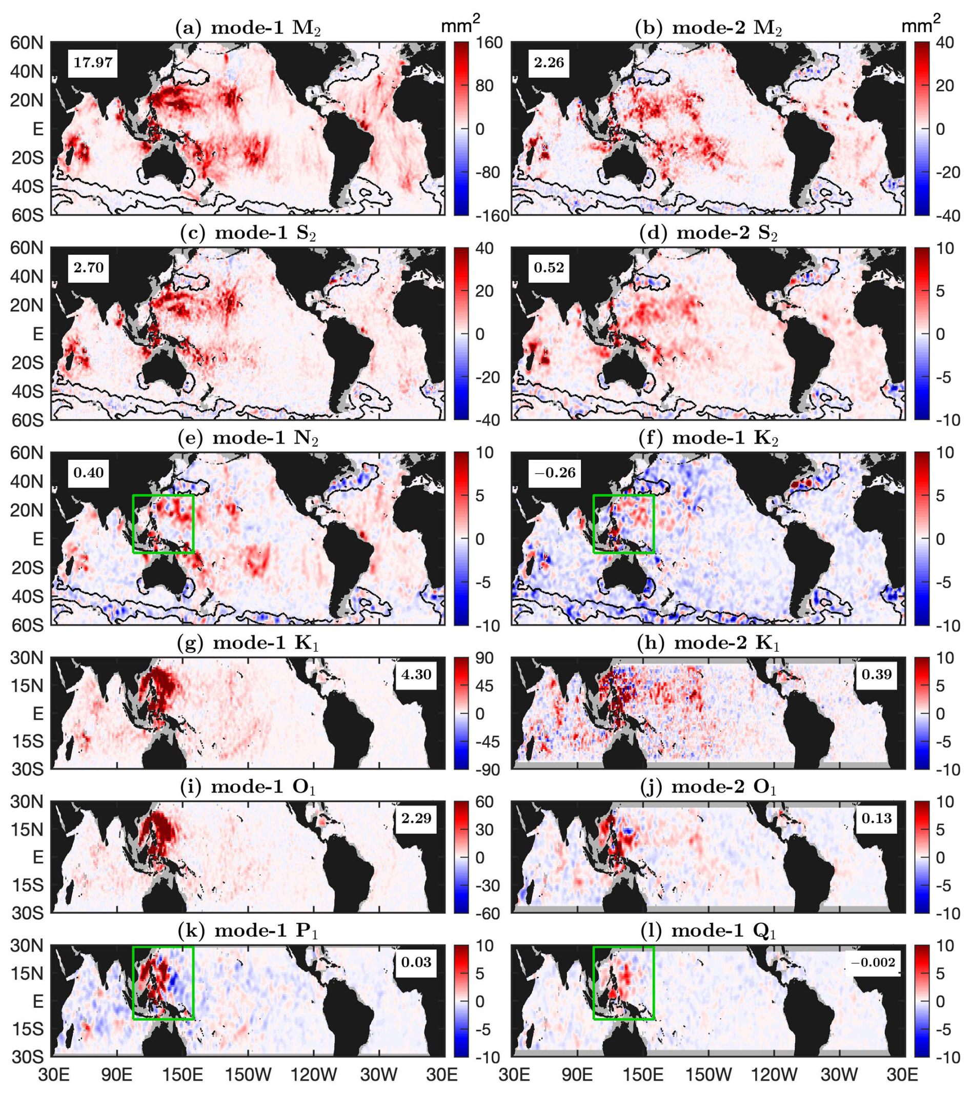
Figure 3Model evaluation. Shown are variance reductions obtained in making internal tide correction to independent altimetry data for 2023. Black contours indicate regions of large model errors. Global area-weighted mean variance reductions (unit: mm2) are given in the upper left (a–f) and right (g–l) corners. Green boxes indicate regions where minor constituents have strong signals.
4.3 Comparison of ZHAO20yr and ZHAO30yr
In this section, I show that ZHAO30yr is greatly improved over ZHAO20yr, an old model developed in Zhao et al. (2016) and presented in Carrere et al. (2021). ZHAO20yr was constructed using 20 years of altimetry data from 1993–2012 by the obsolete mapping procedure (Zhao et al., 2016). ZHAO20yr contains only four mode-1 constituents: M2, S2, K1, and O1. Both models are evaluated using the altimetry data for 2023 following the same procedure. The resulting global variance reduction maps (not shown) are similar to Fig. 3. It is straightforward to calculate the global area-weighted mean variance reductions caused by the two models (Fig. S16). It shows that ZHAO30yr reduces more variance than ZHAO20yr for all four constituents. The improvement can be quantified by the change rate of variance reduction following . They are 32 % (M2), 80 % (S2), 45 % (K1), and 36 % (O1), suggesting that ZHAO30yr is significantly improved over my old model. The improvement is mainly because ZHAO30yr is constructed using a longer data record and an improved mapping technique.
A comparison of the mode-1 S2 internal tides in ZHAO20yr and ZHAO30yr is shown in Fig. S17. One can see that ZHAO30yr has a higher spatial resolution and lower errors. The low model errors in ZHAO30yr are evidenced by the weak signals in the regions of large model errors. The improvement is because they are constructed using different altimetry data records. ZHAO20yr uses 20 years of altimetry data from 1993 to 2012 excluding Sun-synchronous missions. The merged data record is only about 60 years long. ZHAO30yr uses all satellite altimetry data from 1993 to 2022 including the Sun-synchronous missions (Fig. 1). The merged data record is about 120 years long, about 2 times longer. Due to their different data densities, the S2 constituent is mapped using fitting windows of 120 and 250 km. As a result, ZHAO30yr has a much higher spatial resolution and better resolved internal tidal beams.
In this section, I present the 12 internal tide constituents, each of which has been divided into two components by propagation direction. The decomposed components reveal numerous well-defined long-range internal tidal beams. A picture is worth a thousand words. An interested reader may study the decomposed internal tide components for more features.
5.1 Mode-1 and mode-2 M2 constituents
Figure 4 shows the mode-1 M2 constituent and its northward (0–180°) and southward (180–360°) components. In this figure, bottom topographic features are indicated by the 3000 m isobath contours (green lines). The five-wave summed M2 internal tide field (Fig. 4a) shows significant small-scale spatial variations caused by multiwave interference. Internal tides with amplitudes lower than 1 mm (model errors) are shown in light blue. Figure 4a shows that mode-1 M2 internal tides are dominantly greater than model errors and barely affected by model errors. Therefore, previous satellite investigations of internal tides mainly focused on the mode-1 M2 constituent. Figure 4a shows that strong mode-1 M2 internal tides occur around the Hawaiian Ridge, around the French Polynesian Ridge, in the western Pacific Ocean, in the Madagascar–Mascarene region, and in the Indonesian Seas. These regions have long been recognized in previous studies by satellite altimetry (Ray and Zaron, 2016; Zhao et al., 2016; Zaron, 2019), numerical models (Simmons et al., 2004; Li et al., 2015; Arbic et al., 2018), semi-analytical models (Nycander, 2005; Falahat et al., 2014; de Lavergne et al., 2019), and recent drifter measurements (Zaron and Elipot, 2024).
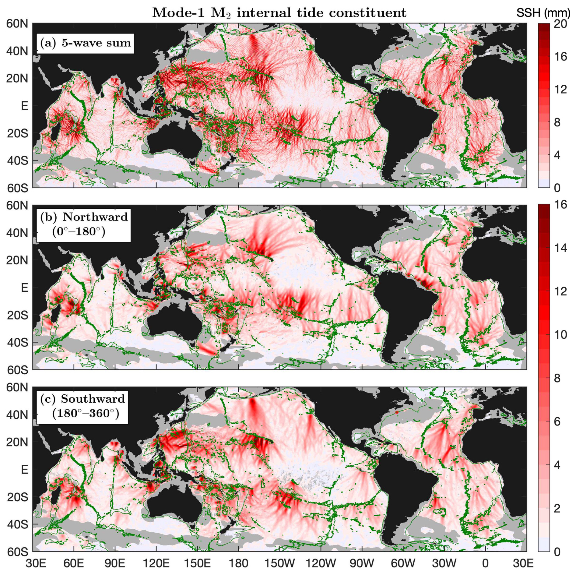
Figure 4Mode-1 M2 internal tide constituent. (a) The five-wave sum. (b) Northward component. (c) Southward component. Internal tides in regions of large model errors or shallower than 1000 m in depth are shown in gray. Green contours indicate the 3000 m isobath. Numerous well-defined long-range internal tidal beams are associated with notable topographic features.
I divide the mode-1 M2 constituent into northward and southward components by propagation direction. The northward and southward components contain the largest waves at each grid point with propagation directions ranging 0–180° and 180–360°, respectively. Such a division can separate long-range internal tidal beams in different directions. Note that the eastward (−90–90°) and westward (90–270°) decomposition can better resolve semidiurnal internal tidal beams in regions such as the western Pacific Ocean. In the decomposed components (Fig. 4b, c), internal tides with amplitudes lower than 23 mm are shown in light blue. The color map adjustment is to highlight internal tidal beams. The northward and southward components show numerous well-defined long-range internal tidal beams, which are featured by larger amplitudes, linear increasing phases, and across-beam co-phase lines (Sect. 6). The results are consistent with previous satellite observations using short data records (Zhao and Alford, 2009; Zhao, 2014; Zhao et al., 2016) because mode-1 M2 internal tides are less affected by model errors.
All mode-1 M2 beams are associated with notable topographic features. In the Pacific Ocean, mode-1 M2 beams radiate from the Hawaiian Ridge, the Line Islands Ridge, the French Polynesian Ridge, the Izu–Bonin–Mariana Arc, the Luzon Strait, the Amukta Pass (Alaska), the Mendocino Ridge, the Macquarie Ridge, and the Eastern Pacific Rise. In the Indian Ocean, mode-1 M2 beams are from the Mascarene Plateau, the Ninety East Ridge, the Andaman island chain, and the Indian western shelf. In the Atlantic Ocean, mode-1 M2 beams are from the Mid-Atlantic Ridge, the Amazon shelf, the Vitória–Trindade Ridge, the Walvis Ridge, the Great Meteor Seamount, and Cape Verde. In addition, there are many short-range mode-1 M2 beams from the narrow straits in the Indonesian Seas, the Coral Sea, and the Caribbean Sea. As an example, Sect. 6.1 shows mode-1 M2 beams off the Amazon shelf.
Figure 5 shows the mode-2 M2 constituent and its northward (0–180°) and southward (180–360°) components. The mode-2 M2 constituent is relatively weak; however, its SSH amplitudes may be up to 15 mm, larger than minor constituents N2 and K2. Mode-2 M2 internal tides are mainly associated with rough bottom topography because they are also generated in the tide–topography interaction. Mode-2 M2 internal tides mainly occur at low latitudes, which is likely determined by the latitudinal structure of ocean stratification. Note that mode-2 M2 internal tides tend to become more incoherent and undetectable because they are easily affected by the time-varying ocean environment. The mode-2 M2 constituent is divided into northward and southward components following the same method. The northward and southward internal tides are to the north and south of notable topographic features, respectively (Fig. 5b, c), suggesting that they are well extracted and separated. The decomposed components show numerous well-defined mode-2 M2 beams. Section 6.1 examines the mode-2 M2 beams off the Amazon shelf.
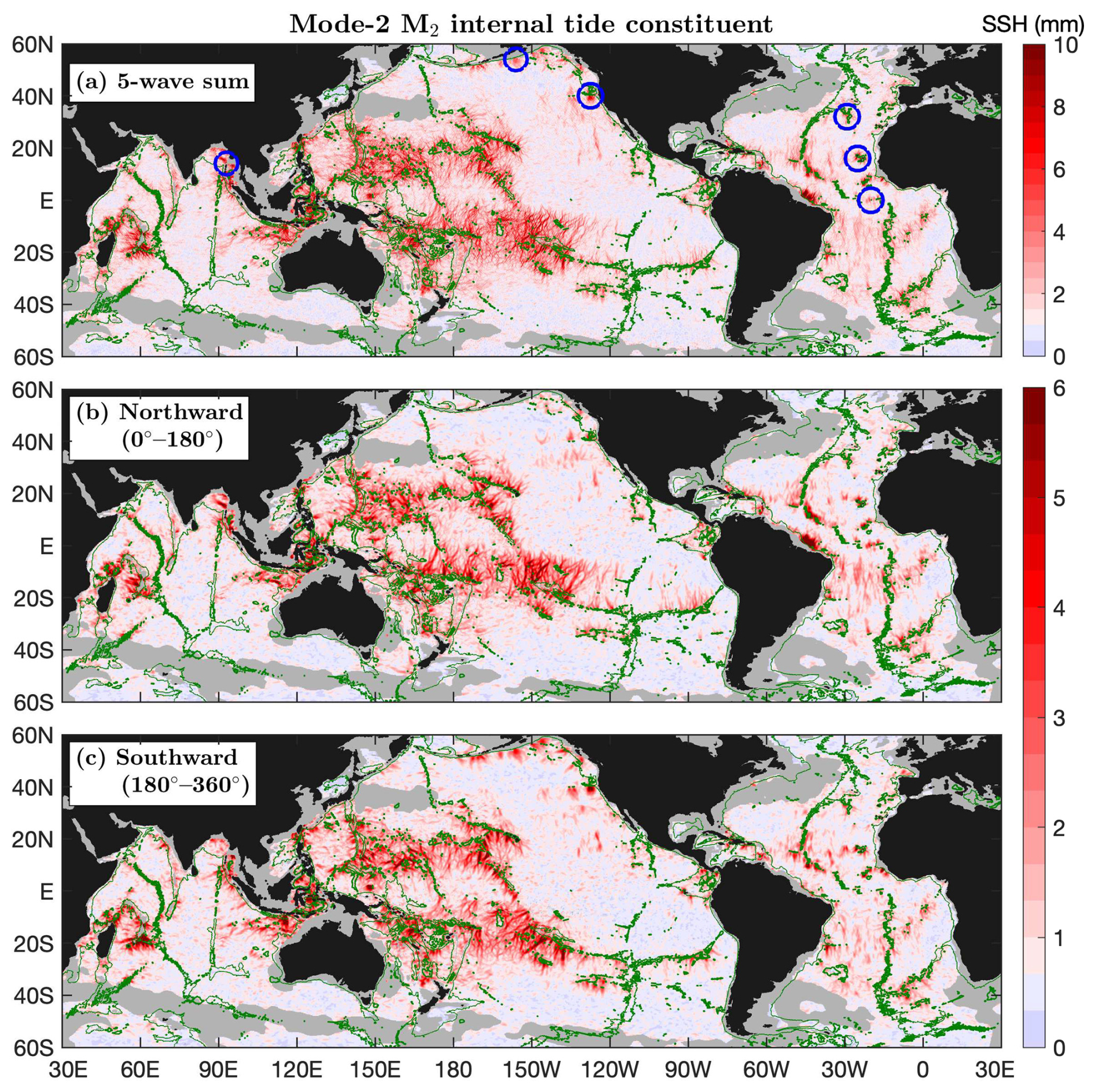
Figure 5As in Fig. 4 but for the mode-2 M2 internal tide constituent. Well-defined long-range internal tidal beams are associated with notable topographic features. Blue circles mark some isolated beams. Mode-2 M2 beams are narrower and shorter than mode-1 M2 beams.
In the Pacific Ocean, the following remarkable generation sources have been recognized: the Hawaii region in the North Pacific, seamounts, island chains and ridges in the western Pacific Ocean, the western South Pacific including the Coral Sea, the French Polynesian Ridge in the South Pacific, the Eastern Pacific Rise, the Alaskan shelf, and the Indonesian Seas. The Indian Ocean has the following remarkable sources: the Madagascar–Mascarene region, the Indian western shelf, the Bay of Bengal, the Andaman Sea, and the Australian northwest coast. In the Atlantic Ocean, mode-2 M2 beams are associated with the Mid-Atlantic Ridge, the Amazon shelf, the Walvis Ridge, and several scattered seamounts. In Fig. 5, some mode-2 M2 beams are highlighted using blue circles. Note that ZHAO30yr presents a better mode-2 M2 field than Zhao (2018) due to the long data record and improved mapping technique (Sects. 2 and 3).
The satellite-observed mode-1 and mode-2 M2 beams have the following different features. (1) Mode-2 M2 beams are shorter than mode-1 M2 beams. Mode-2 M2 internal tides can travel over hundreds of kilometers, in contrast to thousands of kilometers for mode-1 M2 internal tides. It is partly because mode-2 waves become more incoherent than mode-1 waves after leaving their generation sources (Rainville and Pinkel, 2006). (2) Mode-2 M2 beams are narrower than mode-1 M2 beams. That is why the altimetry data along nonrepeat tracks are important in mapping mode-2 internal tides. (3) There are more mode-2 M2 beams than mode-1 M2 beams, likely because mode-2 M2 beams can be induced by small-scale topographic features such as isolated seamounts (Llewellyn Smith and Young, 2002; Zhao, 2018; Geoffroy et al., 2024). Because mode-2 M2 beams are narrower and shorter, one can locate their sources over topographic features. For example, some isolated mode-2 beams are unambiguously associated with known topographic features (Fig. 5, blue circles). The mode-1 and mode-2 M2 beams shown in Figs. 4 and 5 contain a lot of important information. A detailed examination of the M2 internal tides region by region or beam by beam can deepen the understanding of their generation, propagation, and dissipation.
5.2 Mode-1 and mode-2 S2 constituents
Figure 6 shows the mode-1 S2 constituent and its northward (0–180°) and southward (180–360°) components. Similar to the mode-1 M2 constituent, the decomposed components (Fig. 6b, c) reveal numerous long-range mode-1 S2 internal tidal beams. It shows the northward mode-1 S2 beams from the Hawaiian Ridge reaching the Alaskan shelf and the southward mode-1 S2 beams from Amukta Pass (Alaska) reaching the Hawaiian Ridge. These long-range mode-1 S2 beams have been observed in Zhao (2017). Additionally, mode-1 S2 beams are observed to radiate from notable topographic features such as the Mendocino Ridge, the French Polynesian Ridge, the Izu–Bonin–Mariana Arc, the Australian northwest shelf, the Lombok Strait, the Andaman island chain, and the Mascarene Plateau. In the Atlantic Ocean, mode-1 S2 beams radiate from the Amazon shelf, the Vitória–Trindade Ridge, the Walvis Ridge, and isolated seamounts along the Mid-Atlantic Ridge. Compared to Zhao (2017), however, ZHAO30yr can better resolve mode-1 S2 beams due to its higher spatial resolution and lower noise level. In general, the mode-1 M2 and S2 constituents show similar internal tidal beams. For example, one notable topographic feature (e.g., the Hawaiian Ridge) usually generates both M2 and S2 internal tidal beams. But they have the following different features. (1) Mode-1 S2 beams are usually narrower and shorter than corresponding mode-1 M2 beams, likely because the S2 barotropic and internal tides are weak and easily masked by model errors. (2) Mode-1 S2 internal tides in the southern Pacific Ocean (e.g., the French Polynesian Ridge, the Tasman Sea, and the Coral Sea) are weaker, which is caused by the weaker S2 barotropic tide in this region (Zhao, 2017).
Figure 7 shows the mode-2 S2 constituent and its northward (0–180°) and southward (180–360°) components. The mode-2 S2 constituent is much weaker. Its amplitudes are usually lower than 4 mm. Therefore, in most of the global ocean, mode-2 S2 internal tides are overwhelmed by model errors. Fortunately, mode-2 S2 internal tides are strong enough to overcome model errors in their source regions such as the Hawaiian Ridge, the western Pacific Ocean, the Indonesian Sea, the Coral Sea, the Madagascar–Mascarene region, and the Amazon shelf. Note that the 2–3-mm mode-2 S2 internal tides are real signals because they can cause positive variance reductions in making internal tide correction to independent altimetry data (Fig. 3d). Likewise, the decomposed components (Fig. 7b, c) show numerous well-defined mode-2 S2 beams associated with topographic features. For example, one mode-2 S2 beam radiates from the Andaman island chain (Fig. 7b, blue circle). Mode-2 S2 beams can be clearly seen off the Amazon shelf (Sect. 6.1). In conclusion, the mode-1 and mode-2 S2 constituents are weak; however, my multiwave decomposition can resolve well-defined internal tidal beams.
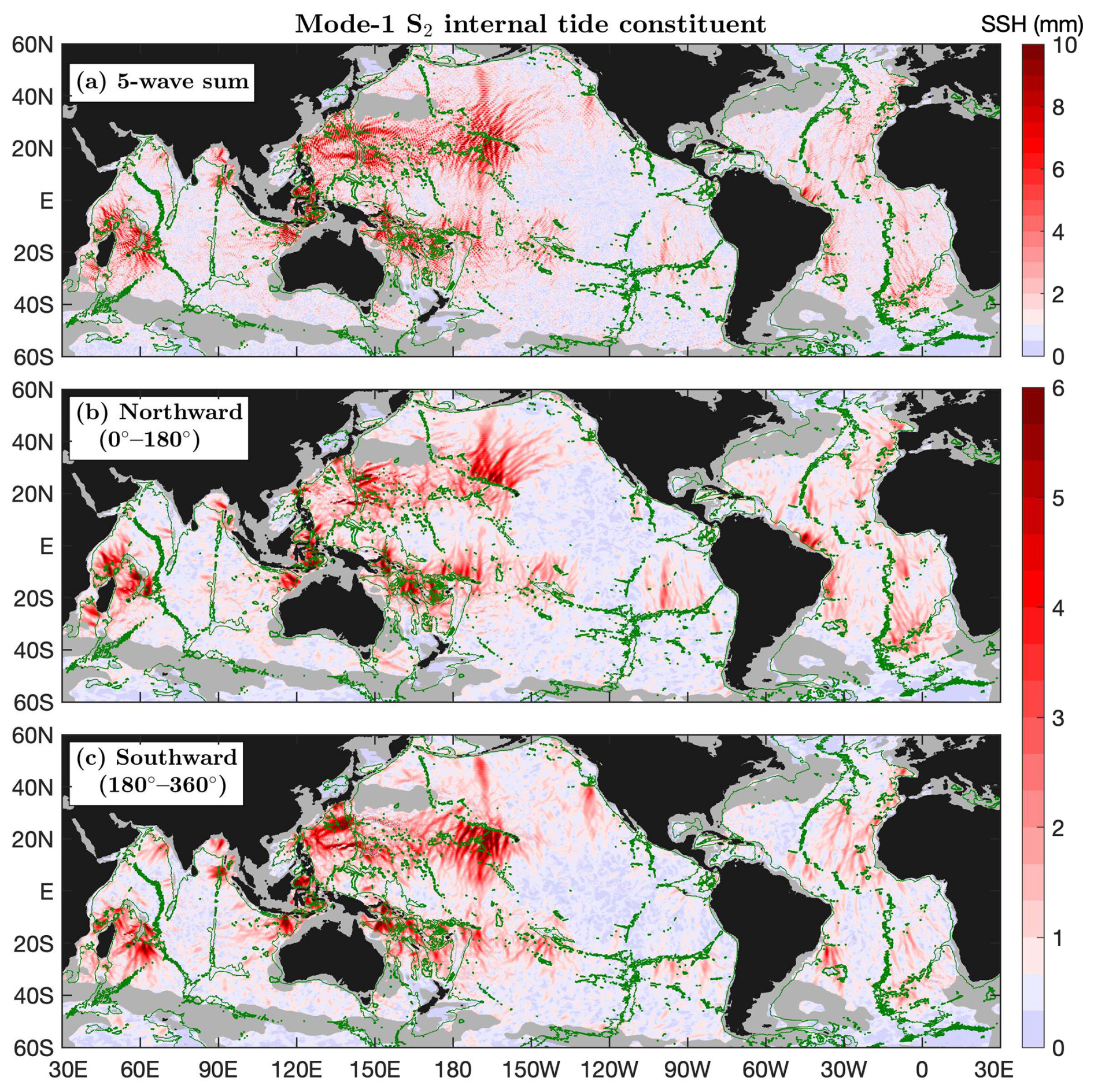
Figure 6As in Fig. 4 but for the mode-1 S2 internal tide constituent.
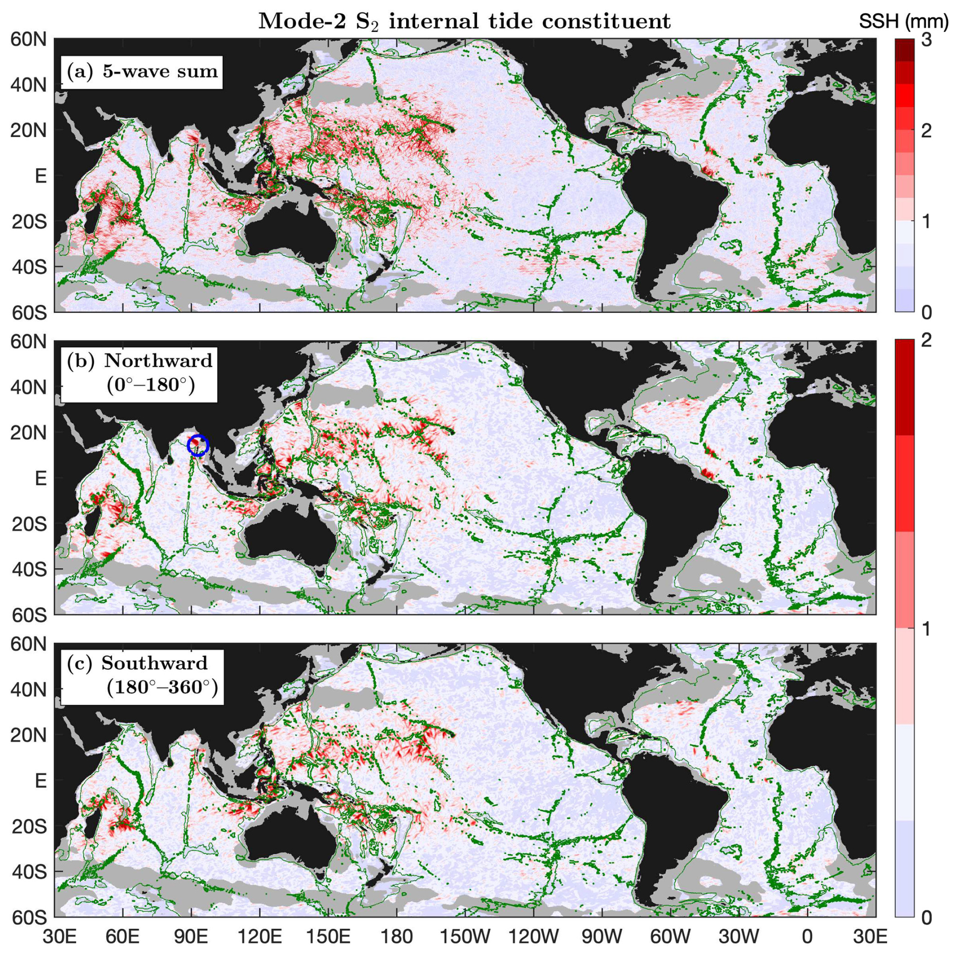
Figure 7As in Fig. 5 but for the mode-2 S2 internal tide constituent. The blue circle marks an isolated beam in the Bay of Bengal.
5.3 Mode-1 N2 constituent
Figure 8 shows the mode-1 N2 constituent and its northward (0–180°) and southward (180–360°) components. The mode-1 N2 constituent has amplitudes as large as 6 mm and can overcome model errors in most of the global ocean. Mode-1 N2 beams can be seen in the five-wave summed field (Fig. 8a), but they are smeared by multiwave interference. The decomposed components (Fig. 8b, c) reveal well-defined long-range mode-1 N2 beams. For example, one can observe both northward and southward N2 beams radiating from the Hawaiian Ridge, the French Polynesian Ridge, and the Macquarie Ridge. In an earlier work, Zhao (2023b) mapped the mode-1 N2 constituent using 27 years of altimetry data (1993–2019) by the same mapping technique used in this study. A comparison shows that the two models are almost the same because 90% of the two data records are the same (27-year vs. 30-year). Zhao (2023b) gave a detailed description of the mode-1 N2 constituent and compared it with the mode-1 M2 constituent. It was reported that mode-1 N2 internal tides can travel from the Hawaiian Ridge to Alaska and that the southward beams from the Mendocino Ridge can travel over 2000 km. Zhao (2023b) showed that mode-1 M2 and N2 internal tides have similar spatial patterns and that the N2 amplitudes are about of the M2 amplitudes. To avoid repetition, an interested reader is referred to Zhao (2023b) for a detailed description of the mode-1 N2 constituent.
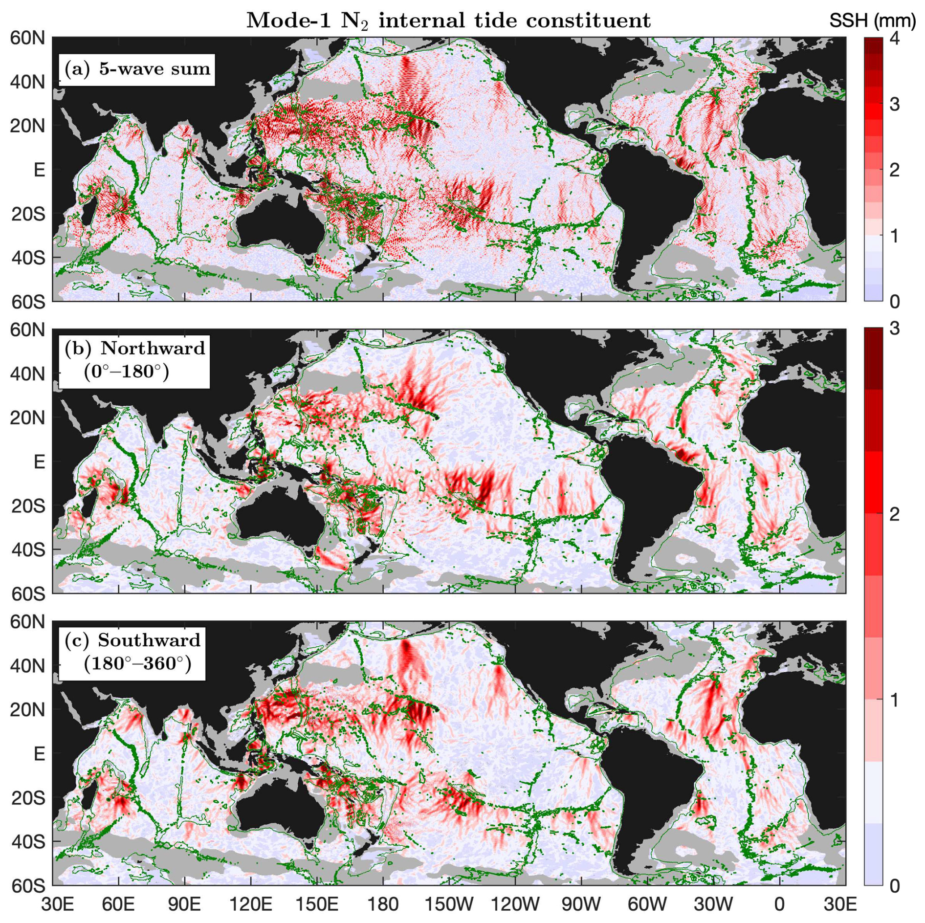
Figure 8As in Fig. 4 but for the mode-1 N2 internal tide constituent.
5.4 Mode-1 K2 constituent
Figure 9 shows the mode-1 K2 constituent and its northward (0–180°) and southward (180–360°) components. The weak mode-1 K2 constituent usually has amplitudes lower than 4 mm; therefore, it is masked by model errors in most of the global ocean. However, the mode-1 K2 constituent can overcome model errors in its source regions such as the Hawaiian Ridge, the Indonesian Seas, and the western Pacific Ocean, where positive variance reduction is obtained in making internal tide correction to independent altimetry data. The decomposed components show numerous well-defined mode-1 K2 beams. For example, one can see southward and northward beams from the Hawaiian Ridge. Note that mode-1 K2 beams from the Hawaiian Ridge can be tracked over 1000 km before disappearance. In addition, mode-1 K2 beams radiate from the Mascarene Plateau, the Luzon Strait, the Mendocino Ridge, the Lombok Strait, the Vitória–Trindade Ridge, and the Amazon shelf (Sect. 6.1).
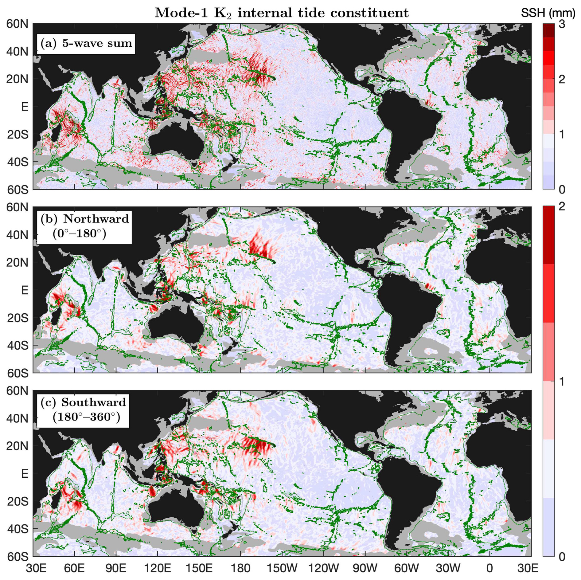
Figure 9As in Fig. 4 but for the mode-1 K2 internal tide constituent.
5.5 Mode-1 and mode-2 K1 constituents
Figure 10 shows the mode-1 K1 constituent and its eastward (−90–90°) and westward (90–270°) components. In this study, all diurnal internal tide constituents are divided into eastward and westward components because such a division can better resolve internal tidal beams in most of the global ocean. The eastward and westward components contain the largest wave at each grid point with propagation direction ranging −90–90° and 90–270°, respectively. All diurnal internal tide constituents are limited within about ±30°, poleward of which there are no propagating diurnal internal tides. The 3000 m isobath contours are overlain to show topographic features. The most remarkable feature of the mode-1 K1 constituent and other diurnal constituents is their geographic distribution: all diurnal constituents are strong in the Indian Ocean and western Pacific Ocean and weak in the Atlantic Ocean and eastern Pacific Ocean. This feature stems from the geographic inhomogeneity of the diurnal barotropic tide (Egbert and Ray, 2003). It has long been known that the diurnal barotropic tide is weak in the Atlantic Ocean.
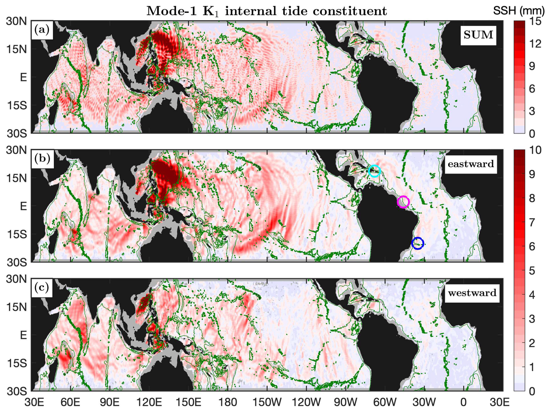
Figure 10Mode-1 K1 internal tide constituent. (a) The five-wave sum. (b) Eastward component (−90–90°). (c) Westward component (90–270°). Internal tides in regions shallower than 1000 m in depth are shown in gray. Well-defined long-range mode-1 K1 beams are associated with notable topographic features. Colored circles mark isolated mode-1 K1 beams in the Atlantic Ocean: the Mona Passage (cyan), the Amazon shelf (magenta), and the Vitória–Trindade Ridge (blue).
The Luzon Strait is the strongest source of mode-1 K1 internal tides and radiates mode-1 K1 beams eastward into the western Pacific Ocean and westward into the South China Sea. In their long-range propagation, both beams refract toward the Equator due to the beta effect (Zhao, 2014). The Tonga–Kermadec Ridge radiates another long-range mode-1 K1 beam that propagates northeastward over 3000 km and refracts toward the Equator for the same reason (Fig. 10b). The decomposed components (Fig. 10b, c) show numerous well-defined long-range mode-1 K1 beams. In the Indian Ocean, mode-1 K1 beams radiate from the Indian western shelf, the Ninety East Ridge, the Andaman island chain, and the Mascarene Plateau. In the Pacific Ocean, mode-1 K1 beams are from the Luzon Strait, the Indonesian Seas, the Hawaiian Ridge, the Line Islands Ridge, the French Polynesian Ridge, and the Eastern Pacific Rise. In the Atlantic Ocean, weak but well-defined mode-1 K1 beams are observed in the Caribbean Sea. Among them, the K1 internal tidal beam from the Mona Passage (Fig. 10b, cyan circle) has been well studied previously (Dushaw, 2006; Dushaw and Menemenlis, 2023). One can see weak mode-1 K1 beams offshore of the Amazon shelf (magenta circle) and northward of the Vitória–Trindade Ridge (blue circle).
Figure 11 shows the mode-2 K1 constituent and its eastward (−90–90°) and westward (90–270°) components. The weak mode-2 K1 constituent has amplitudes up to 5 mm. The Luzon Strait is a strong source of mode-2 K1 internal tides. The decomposed components (Fig. 11b, c) show numerous mode-2 K1 beams associated with notable topographic features. For example, westward mode-2 K1 beams occur in the Arabian Sea (Sect. 6.2), where the beams are from the Chagos–Laccadive Ridge and the western shelf of India. In the Indian Ocean, mode-2 K1 beams radiate from the Ninety East Ridge, the Andaman island chain, and the Mascarene Plateau. In the Pacific Ocean, mode-2 K1 beams are from the Luzon Strait, the Indonesian Seas, the Hawaiian Ridge, the Line Islands Ridge, the French Polynesian Ridge, and the Eastern Pacific Rise. In the Atlantic Ocean, the mode-2 K1 internal tides are very weak.
The mode-1 and mode-2 K1 constituents have different spatial patterns (Figs. 10 and11). Mode-2 K1 beams are shorter and narrower than mode-1 K1 beams. The short and narrow mode-2 K1 beams allow us to locate their generation sites. As an example, there are two isolated mode-2 K1 beams in the eastern Pacific Ocean (Fig. 11, blue circles). They originate at two notable seamounts and propagate northward over 1000 km. In contrast, there are no other large diurnal mode-2 beams in the vast eastern Pacific Ocean. This feature raises the question of what special topographic and tidal conditions combined induce these isolated beams. Answering this question may improve the understanding of the generation of internal tides and their variation with global ocean changes.
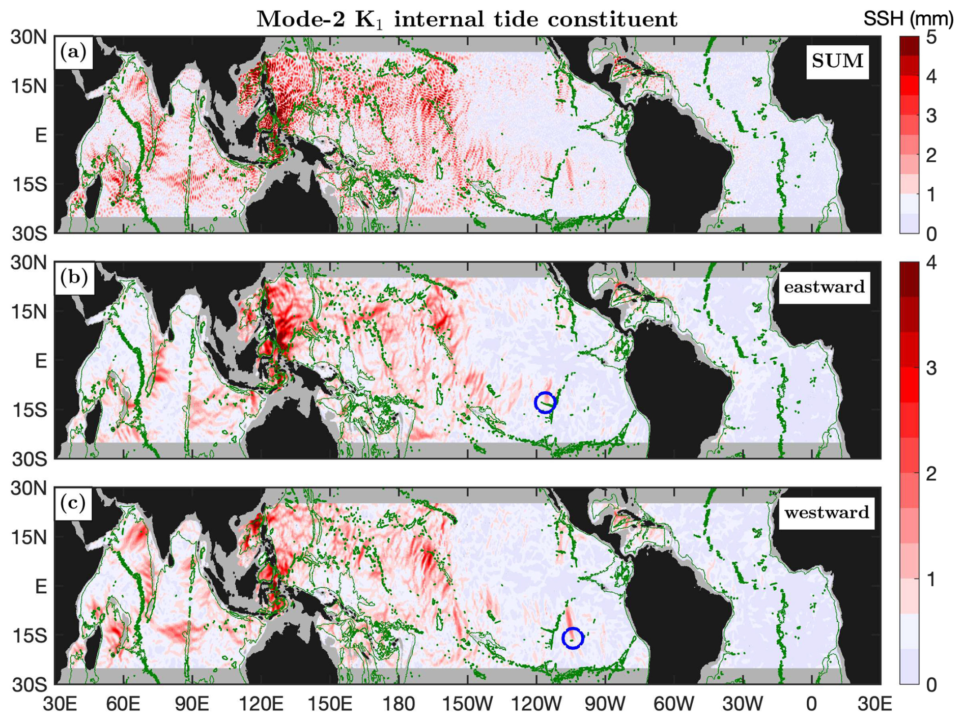
Figure 11As in Fig. 10 but for the mode-2 K1 internal tide constituent. Blue circles mark two isolated beams in the eastern Pacific Ocean.
5.6 Mode-1 and mode-2 O1 constituents
Figure 12 shows the mode-1 O1 constituent and its eastward (−90–90°) and westward (90–270°) components. The mode-1 O1 and K1 constituents have similar spatial patterns (Figs. 10 and 12; correlation coefficient is 0.79), but the K1 constituent is about 50 % stronger in amplitude. The decomposed components (Fig. 12b, c) reveal numerous well-defined long-range mode-1 O1 beams. The Luzon Strait generates the strongest mode-1 O1 internal tides, which propagate eastward into the western Pacific Ocean and westward into the South China Sea. Like mode-1 K1 beams, the two long-range beams refract in propagation due to the beta effect. The Tonga–Kermadec Ridge radiates a strong northeastward mode-1 O1 beam, which travels over 2000 km and refracts in propagation. Another similar feature with mode-1 K1 is that mode-1 O1 internal tides are weak in the Atlantic Ocean and eastern Pacific Ocean and strong in the Indian Ocean and western Pacific Ocean. In the Indian Ocean, mode-1 O1 beams are from the Indian western shelf, the Chagos–Laccadive Ridge, the Mascarene Plateau, and the Ninety East Ridge. Although the O1 amplitudes are low, well-defined mode-1 O1 beams are observed from the Amazon shelf, the Vitória–Trindade Ridge, and the Sierra Leone Rise in the Atlantic Ocean (Fig. 12, blue circles).
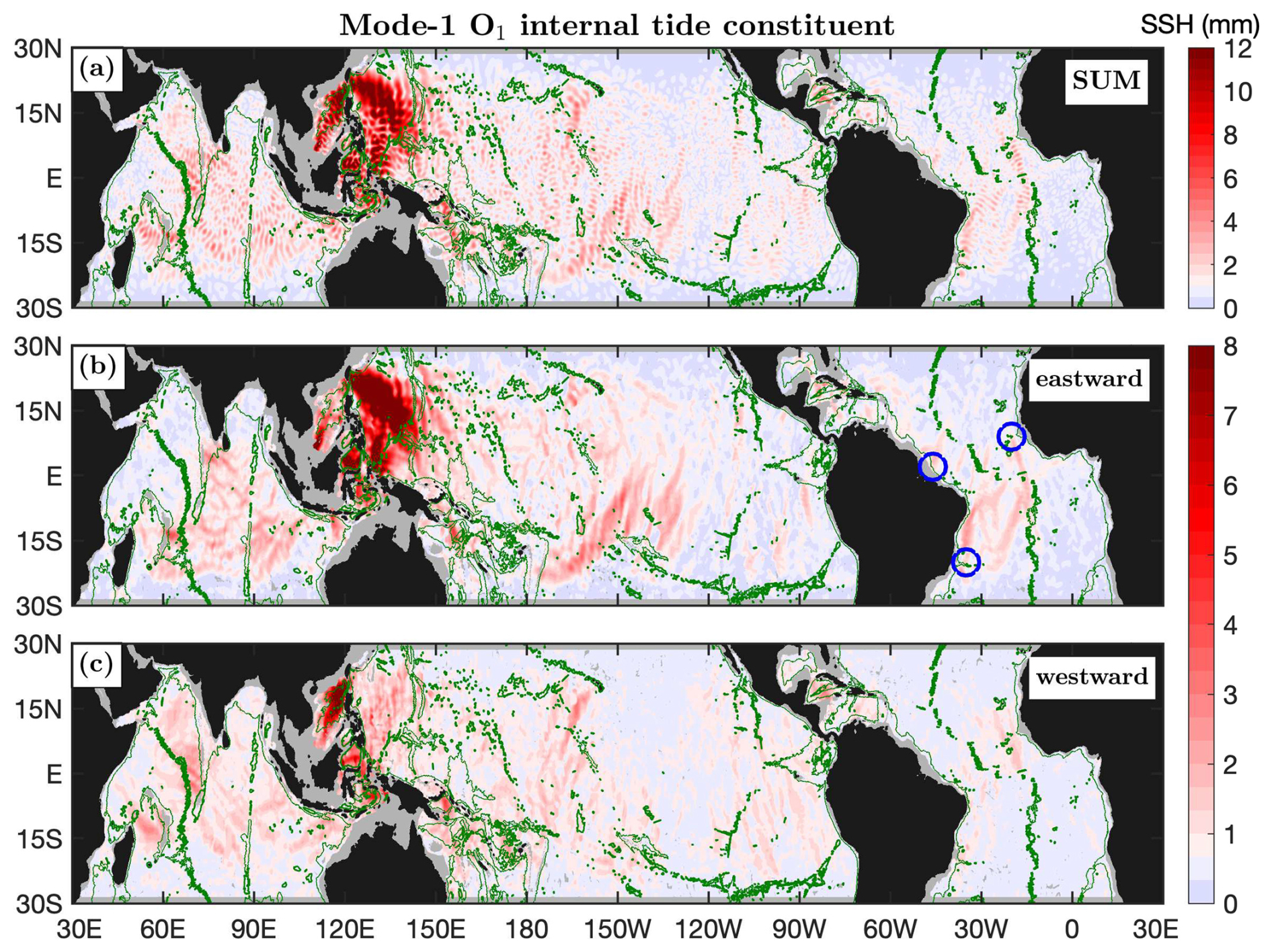
Figure 12As in Fig. 10 but for the mode-1 O1 internal tide constituent. Blue circles mark isolated mode-1 O1 beams.
Figure 13 shows the mode-2 O1 constituent and its eastward (−90–90°) and westward (90–270°) components. The mode-2 O1 and K1 constituents have some degree of similarity, with a correlation coefficient of 0.56. The mode-2 O1 amplitudes are up to 5 mm around the Luzon Strait. Like other diurnal constituents, the mode-2 O1 constituent is strong in the Indian Ocean and western Pacific Ocean. Strong mode-2 O1 internal tides occur in the Indonesian Seas and around the Luzon Strait. Mode-2 O1 beams are also from the Line Islands Ridge and the Izu–Bonin–Mariana Arc. In the eastern Pacific Ocean, there are two singular mode-2 O1 beams (Fig. 13, blue circles), overlapping with the two mode-2 K1 beams (Fig. 11, blue circles). In the Indian Ocean, mode-2 O1 beams are from the Indian western shelf, the Chagos–Laccadive Ridge, the Mascarene Plateau, and the Ninety East Ridge (Sect. 6.2). In the Atlantic Ocean, there is one outstanding beam propagating northward along the Brazilian shelf. In summary, the mode-1 and mode-2 O1 constituents are similar to the mode-1 and mode-2 K1 constituents, respectively, but the K1 constituents are about 50 % larger than the O1 constituents.
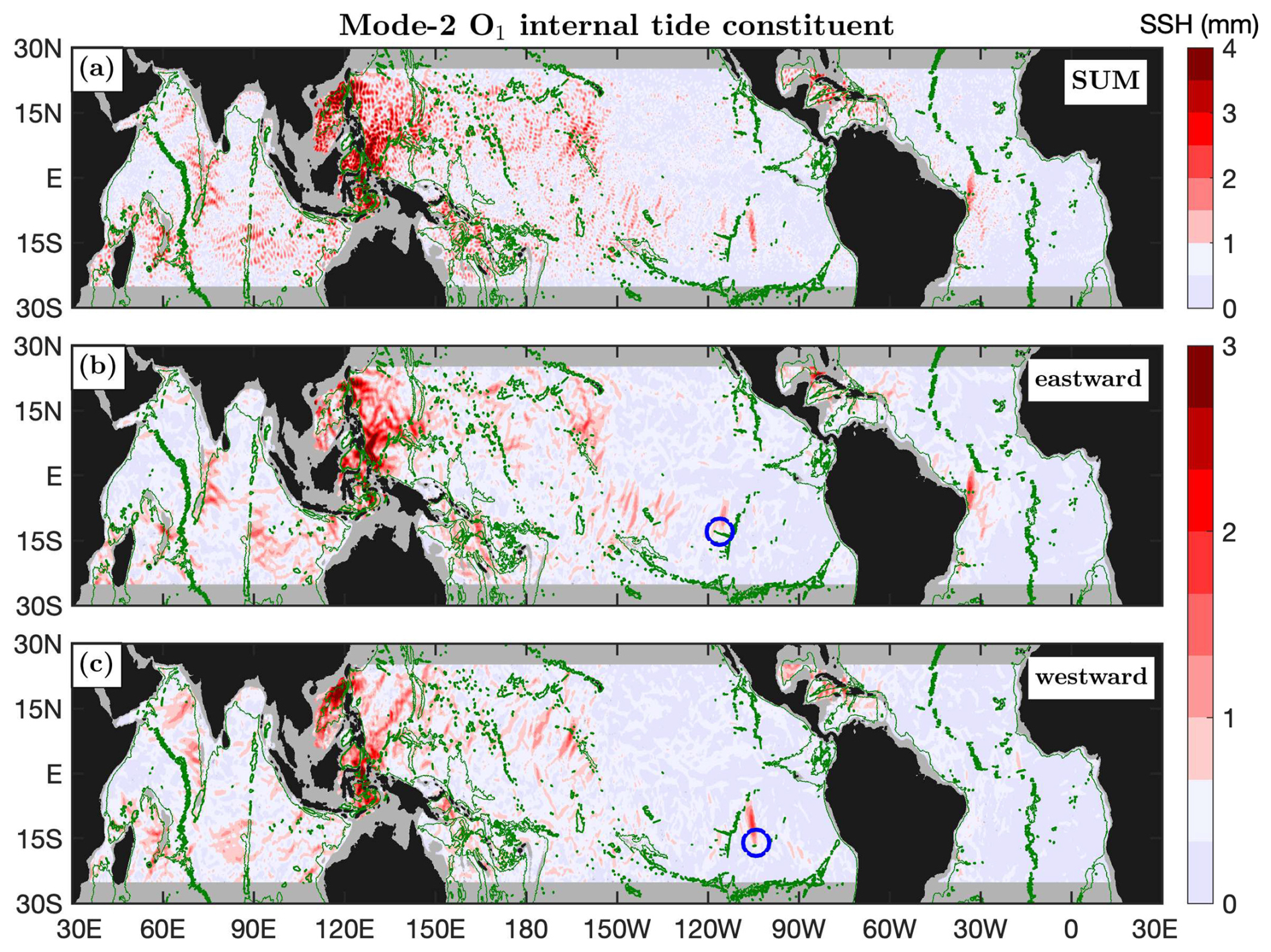
Figure 13As in Fig. 11 but for the mode-2 O1 internal tide constituent. Blue circles mark two isolated beams in the eastern Pacific Ocean.
5.7 Mode-1 P1 constituent
Figure 14 shows the mode-1 P1 constituent and its eastward (−90–90°) and westward (90–270°) components. The mode-1 P1 amplitudes can be up to 5 mm. The Luzon Strait is the strongest generation source and radiates mode-1 P1 beams eastward into the western Pacific Ocean and westward into the South China Sea. The Tango–Kermedac Ridge is another strong generation source and radiates one P1 beam northeastward. Additionally, mode-1 P1 beams are observed from the French Polynesian Ridge and the Hawaiian Ridge. In the Indian Ocean, eastward and westward beams radiate from the Ninety East Ridge. The mode-1 P1 and K1 constituents have similar spatial patterns, and their amplitudes have a scaling factor of about . Note that K1 and P1 are different by 2 cpy in frequency and their superposition forms a semiannual cycle, which should be accounted for in the study of their seasonal variations.
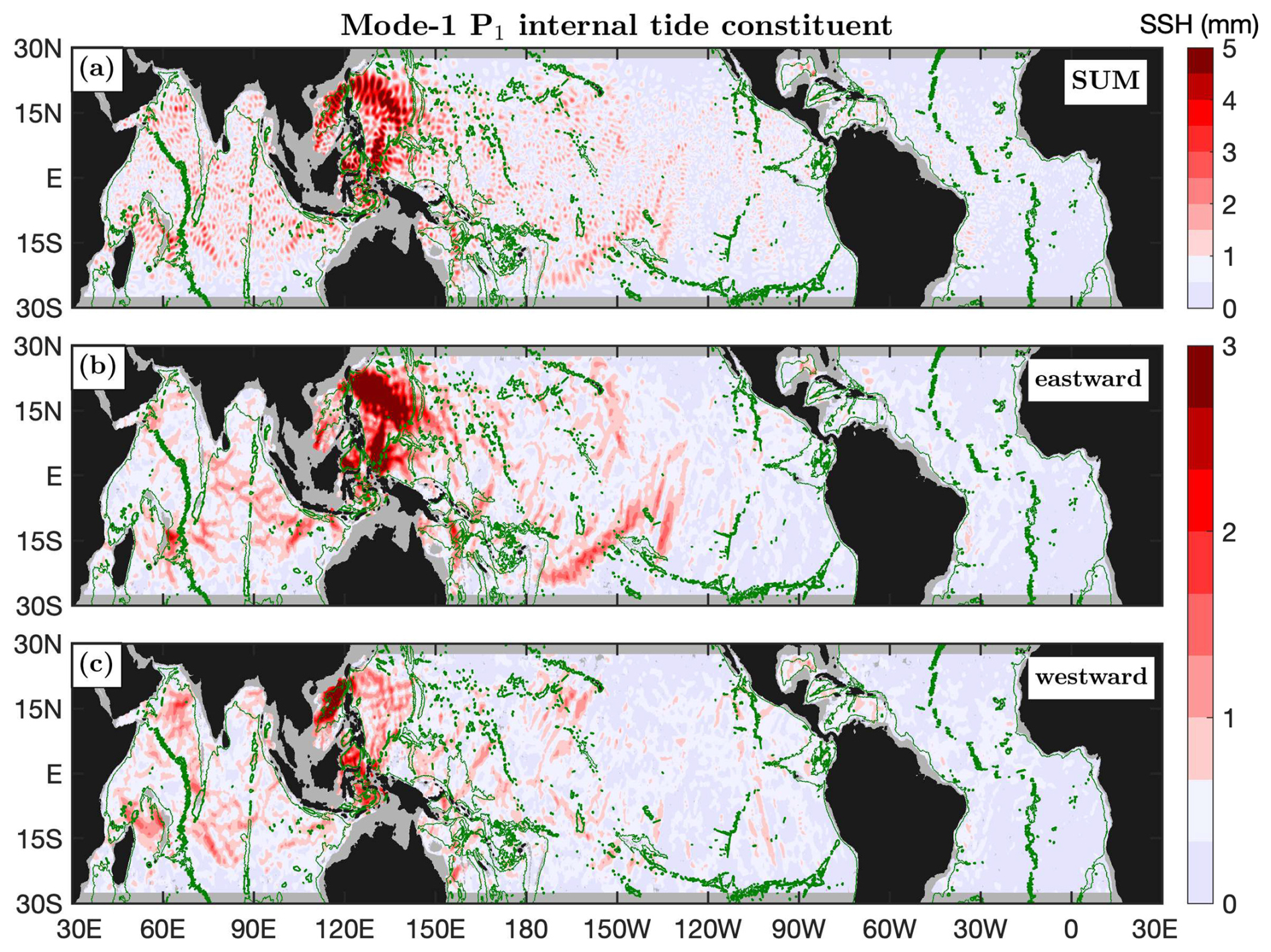
Figure 14As in Fig. 10 but for the mode-1 P1 internal tide constituent.
5.8 Mode-1 Q1 constituent
Figure 15 shows the mode-1 Q1 constituent and its eastward (−90–90°) and westward (90–270°) components. The mode-1 Q1 constituent is very weak and its amplitudes are usually lower than 3 mm. The mode-1 Q1 constituent is overwhelmed by model errors in most of the global ocean. Like other diurnal constituents, the Luzon Strait is the dominant generation source of mode-1 Q1 beams. The Luzon Strait radiates mode-1 Q1 beams eastward into the western Pacific and westward into the South China Sea. One can see strong Q1 internal tides in the Indonesian Seas as well. This feature is consistent with earlier model evaluation (Sect. 4) that Q1 can cause variance reduction in the Indonesian Seas and around the Luzon Strait (Fig. 3).
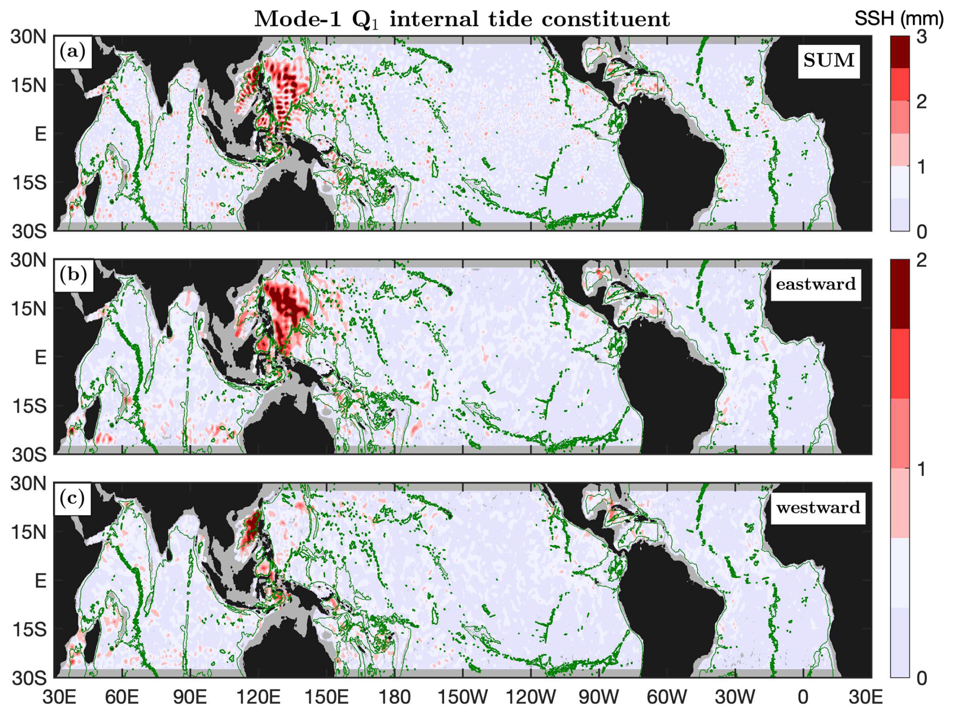
Figure 15As in Fig. 10 but for the mode-1 Q1 internal tide constituent.
The decomposed components show numerous long-range internal tidal beams, which contain important information on their generation and propagation. To better extract the information, one should study them region by region and beam by beam. This section showcases two examples: the semidiurnal beams off the Amazon shelf and the diurnal beams in the Arabian Sea.
6.1 Semidiurnal internal tidal beams off the Amazon shelf
The Amazon shelf (60–35° W, 5° S–20° N) is chosen as an example because of its strong internal tides and frequent occurrence of internal solitary waves (Magalhaes et al., 2016; Barbot et al., 2021; Egbert and Erofeeva, 2021; Tchilibou et al., 2022; de Macedo et al., 2023; Assene et al., 2024). However, previous studies mainly focused on the dominant M2 internal tides. Here I show internal tidal beams for six semidiurnal constituents including mode-1 M2, S2, N2, and K2 and mode-2 M2 and S2. Figure 16 shows the six internal tide constituents in the region. Each constituent is divided into northeastward and southwestward components. The northeastward component contains the largest waves at each grid point with propagation direction ranging −45–135°, and the southwestward component contains the largest waves ranging 135–315° (Fig. S18). The six constituents are shown using the same color map but different ranges because their amplitudes may vary by an order of magnitude. For all constituents, internal tides with low amplitudes are shown in light blue. The 0° co-phase lines are plotted to highlight internal tidal beams.
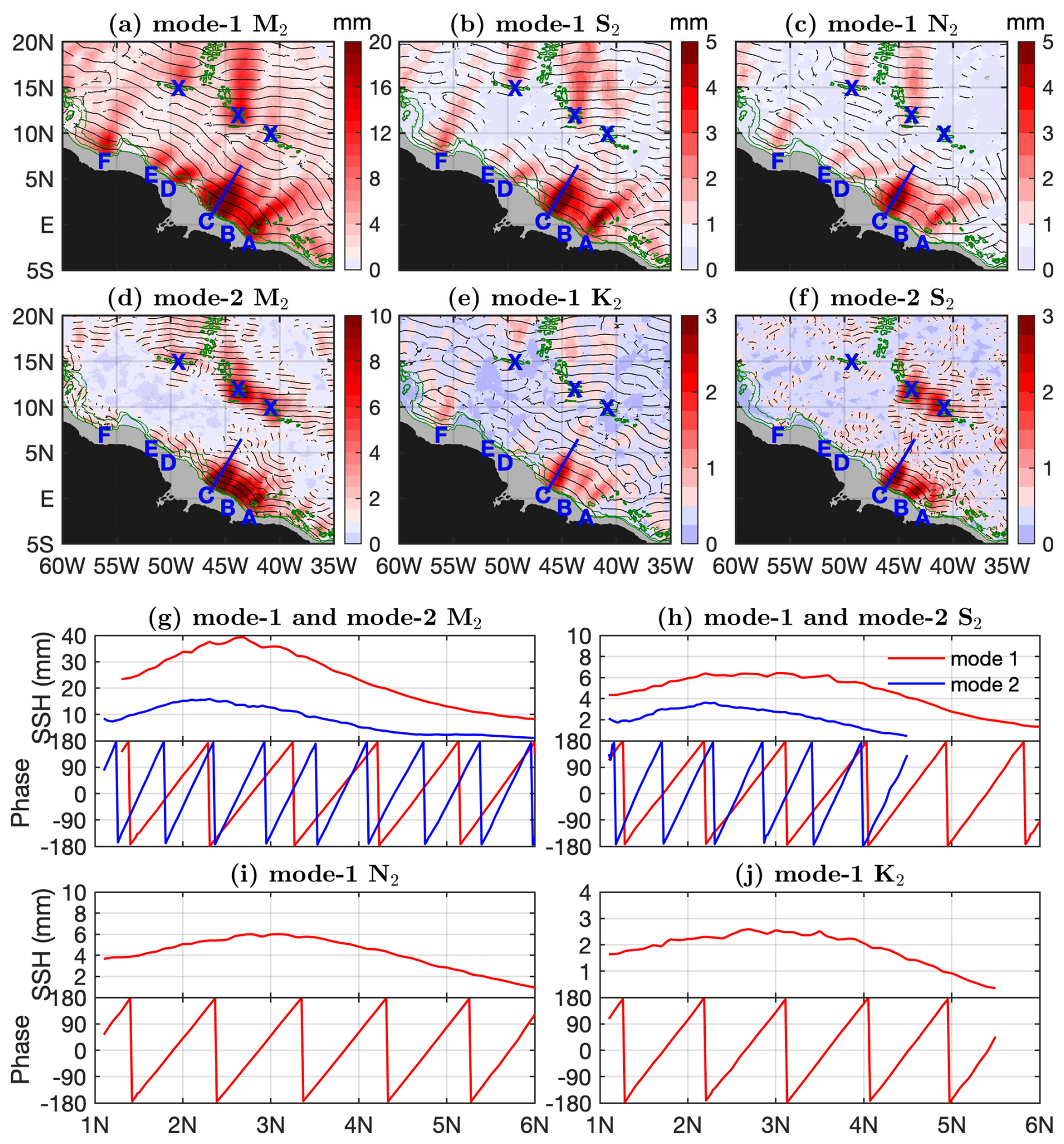
Figure 16Northeastward semidiurnal internal tidal beams off the Amazon shelf. (a–f) Northeastward internal tide components (−45–135°). Black lines indicate the 0° co-phase charts. Green contours indicate the 1000, 2000, and 3000 m isobaths. Each constituent has up to six isolated beams off the Amazon shelf (a–f). Blue lines highlight the strongest beams generated at the mouth of the Amazon River. Beams generated at the Mid-Atlantic Ridge are marked. (g–j) Along-beam amplitudes and phases.
Compared to the multiwave summed products, the decomposed products present a much clearer view of the isolated internal tidal beams off the Amazon shelf. The four mode-1 constituents (M2, S2, N2, and K2) have similar spatial patterns. Among them, M2, S2, and N2 show six isolated internal tidal beams propagating northeastward from the Amazon shelf. They are labeled A–F (Fig. 16). The K2 constituent shows only five beams, A–D and F. Its beam E is missing, most likely because the much weaker K2 (lower than 2 mm) is affected by model errors. The co-phase lines are parallel to one another and across the internal tidal beams. For these constituents, the strongest beams (blue lines) radiate from the mouth of the Amazon River. The along-beam amplitudes and phases are shown in Fig. 16g–j. One can see that their amplitudes are smooth and their phases increase linearly with propagation. These features suggest that these beams are successfully extracted. Otherwise, they would show standing-wave features (half-wavelength fluctuations). Along the strongest beams, their amplitudes range from 40 mm for M2 to 3 mm for K2. The strongest M2 beam can be tracked for about 700 km from the Amazon shelf to the Mid-Atlantic Ridge. For comparison, the S2, N2, and K2 beams disappear sooner, likely because their lower amplitudes are masked by the still large model errors. In addition, my satellite observations also reveal internal tidal beams generated over the Mid-Atlantic Ridge (Fig. 16, “X”). Maximum SSH amplitudes along all beams do not appear on the Amazon shelf but about one wavelength away from their source. It is likely an artificial feature caused by the large spatial windows used in plane wave fitting and Fourier bandpass filtering. It is also likely because the distances are needed for the internal tidal rays to bounce to the sea surface for the first time (Merrifield and Holloway, 2002; Carter et al., 2008).
Our satellite observations are generally consistent with previous numerical simulations, which mainly focused on M2 internal tides. Isolated M2 internal tidal beams are observed by Tchilibou et al. (2022, Fig. 7) and Assene et al. (2024, Fig. 2). For example, Tchilibou et al. (2022) identified six strong internal tidal beams off the Amazon shelf. Their generation sites are consistent with satellite observations. One exception is that they suggest that the strong beam (Fig. 16a, beam C) is composed of two beams. Previous studies found that the strong beams overlap with internal solitary waves very well, in that internal solitary waves are generated by nonlinear internal tides. Tchilibou et al. (2022) showed the temporal variation of internal tides in two contrasting time periods: September–November and March–June. Likewise, M2 internal tide maps have been constructed using four seasonal subsets (Zhao, 2021) and decadal maps (Zhao, 2023a). It would be interesting to compare the satellite observations, numerical models, semi-analytical results, and in situ measurements in future research (Pollmann and Nycander, 2023; Assene et al., 2024; Zaron and Elipot, 2024; Geoffroy et al., 2025). The six beams are spatially collocated for the four constituents, suggesting that they are generated by the same topographic features. Their superposition will lead to the temporal variability of semidiurnal internal tides (strong beats and weak beats).
Our decomposed products also reveal mode-2 M2 and S2 internal tidal beams (Fig. 16d, f). Both constituents show three beams, A–C. There are no outstanding mode-2 beams at D–F. Figure 16g and h show the along-beam amplitudes and phases for mode-2 M2 and S2 (blue lines). It shows that the mode-2 M2 amplitudes may be up to 15 mm, and the mode-2 S2 amplitudes are up to 4 mm. Similarly, the mode-2 beams have large and smooth amplitudes and their phases increase linearly with propagation. The mode-2 M2 constituent is larger than mode-1 S2 and N2 constituents; therefore, the missing beams, D–F, are not likely because of its weak signals. Rather, it is likely that the local specific topography favors the generation of mode-1 constituents, but not mode-2 constituents.
6.2 Diurnal beams in the Arabian Sea
The westward diurnal internal tidal beams in the Arabian Sea are examined next. In this region, the dominant M2 internal tides have been well documented in previous studies (Kaur et al., 2024; Ma et al., 2021; Subeesh and Unnikrishnan, 2016; Subeesh et al., 2021; Zhao, 2021). Figure 17 shows the lowest two modes of the diurnal O1 and K1 constituents. Each constituent is divided into eastward and westward components. The eastward component contains the largest waves at each grid point ranging −90–90° (Fig. S19), and the westward component contains the largest waves ranging 90–270°. Overlain are the 0 and 180° co-phase lines. The intervals between two neighboring co-phase lines are half of one wavelength. Topographic features are indicated by the 1000, 2000, and 3000 m isobaths. My new model reveals isolated long-range internal tidal beams for both O1 and K1.
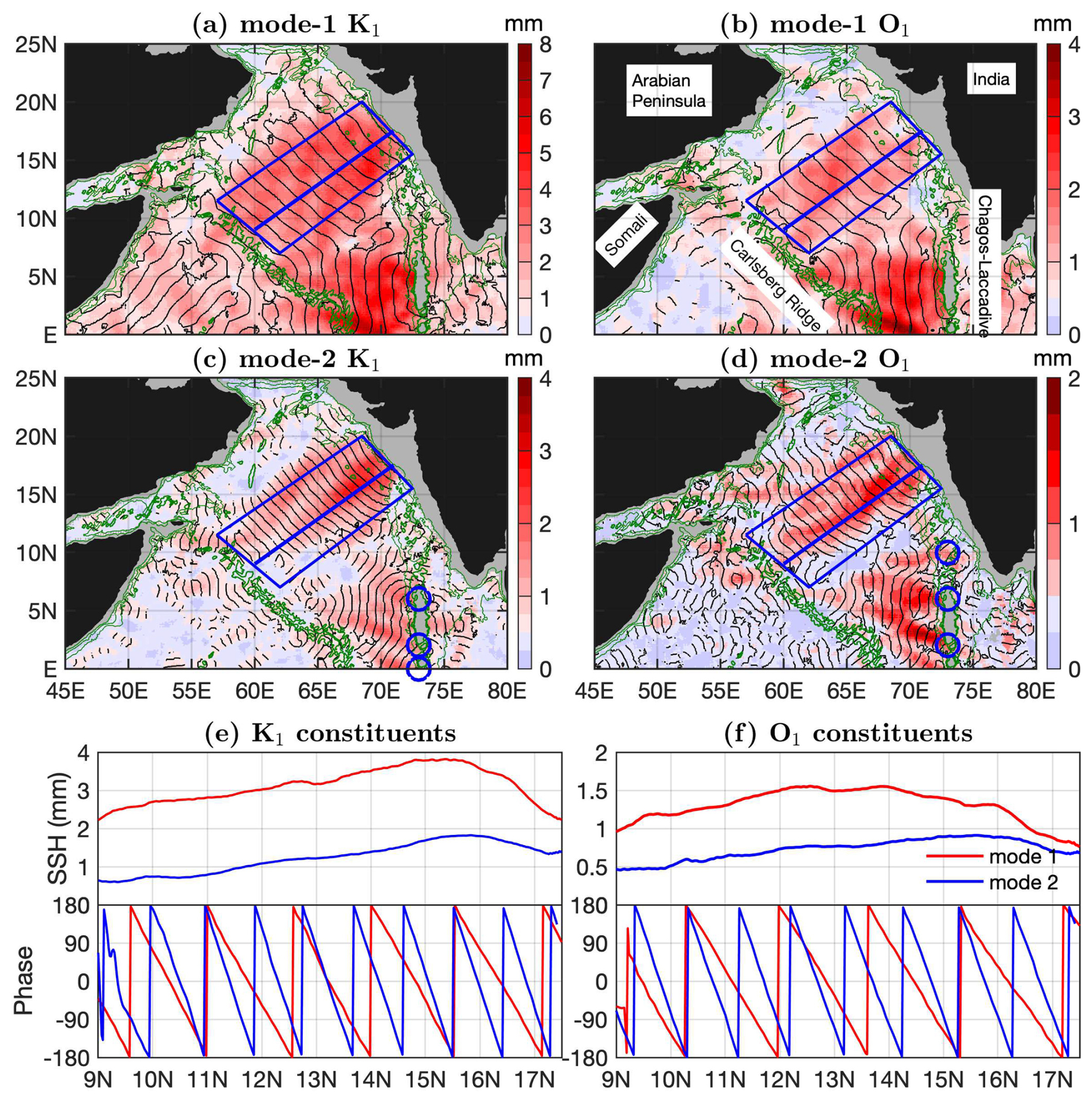
Figure 17Westward diurnal internal tidal beams in the Arabian Sea. (a–d) Westward internal tide components (90–270°). Black lines indicate the 0 and 180° co-phase charts. Internal tides with amplitudes lower than 0.5 mm are shown in light blue. Green contours indicate the 1000, 2000, and 3000 m isobaths. Blue circles mark some isolated mode-2 beams at the Chagos–Laccadive Ridge. (e, f) Along-beam amplitudes (averaged across the beam) and phases (along the central line).
Figure 17 shows that diurnal internal tides have two outstanding generation sites. One set of beams originates at the Indian western shelf along 15–20° N. The beams propagate toward 210° for about 2000 km from the Indian coast to the Carlsberg Ridge. It takes about six (10) repeat diurnal tidal cycles for mode-1 (mode-2) K1 and O1 internal tides to travel across the distance. Another set of beams radiates from the Chagos–Laccadive Ridge (along 73° E) and travels over 1000 km before disappearance. The mode-2 beams from the Chagos–Laccadive Ridge appear to be composed of several isolated narrow beams (blue circles). Note that the two generation sites also generate strong M2 internal tides (Subeesh et al., 2021; Ma et al., 2021). For comparison, the diurnal internal tidal beams are wider than semidiurnal beams. The southwestward mode-2 beams from the Indian western shelf are about 500 km wide.
Figure 17e and f show along-beam amplitudes and phases for the first two modes of the K1 and O1 constituents. Their smooth amplitudes and linear increasing phases suggest that the beams have been successfully separated. The diurnal internal tidal beams have small amplitudes, ranging from 4 mm for mode-1 K1 to 1 mm for mode-2 O1 internal tides. This feature again suggests that my new internal tide model has low model errors. However, the even weaker P1 and Q1 constituents (lower than 1 mm) do not show well-defined internal tidal beams (Figs. 14 and 15). The regional maps reveal isolated beams and generation sites. Such an examination can be conducted constituent by constituent and region by region.
In this work, I have mapped global internal tides by applying my recently improved mapping technique to 30 years of satellite altimetry data from 1993 to 2022 (Fig. 1). My mapping technique consists of two rounds of plane wave analysis with a spatial bandpass filter in between (Zhao, 2022a, b). The data record is 120 satellite years long, including all the nadir altimetry data collected by 15 altimetry missions. My main findings and conclusions are summarized as follows.
-
I have constructed a new internal tide model that contains 12 internal tide constituents (Fig. S3): eight mode-1 constituents (M2, S2, N2, K2, K1, O1, P1, and Q1) and four mode-2 constituents (M2, S2, K1, and O1). The combination of a long data record and an improved mapping technique significantly suppresses model errors down to lower than 1 mm on global average (Fig. 2), which makes it possible to map weak mode-2 and minor internal tide constituents.
-
I have decomposed the multiconstituent, multimodal, multidirectional internal tide field into a series of simple plane waves. In frequency, eight principal constituents are extracted. In the vertical direction, the two lowest baroclinic modes are extracted for the four major constituents. In the horizontal direction, each internal tide constituent is decomposed into five plane waves in different directions. All together, the internal tide field is decomposed into 60 plane waves at each grid point (Figs. S4–S15). The multiwave decomposition reveals a new view of the global internal tide field.
-
I have validated the new internal tide model using independent altimetry data for 2023 (Fig. 3). On global average, 10 constituents (but for K2 and Q1) can cause positive variance reductions because these constituents are sufficiently strong to overcome model errors. The weak K2 and Q1 constituents can overcome model errors near their sources in the western Pacific Ocean.
-
I have shown that ZHAO30yr performs much better than ZHAO20yr (Figs. S16 and S17), a model developed using 20 years of altimetry data by an obsolete mapping technique (Zhao et al., 2016). The improvement is mainly because ZHAO30yr is developed using a longer data record and an improved mapping technique.
-
I have observed numerous isolated internal tidal beams for all 12 internal tide constituents. Their decomposed components reveal well-defined long-range internal tidal beams (Figs. 4–15). These beams are associated with notable topographic features. For all constituents, mode-2 beams are shorter and narrower than corresponding mode-1 beams. One can acquire important information on their generation, propagation, and dissipation by tracking these long-range internal tidal beams.
-
I have studied the semidiurnal internal tidal beams off the Amazon shelf (Fig. 16). For mode-1 constituents (M2, S2, N2, and K2), six isolated beams propagating northeastward off the Amazon shelf have been recognized. Along the strongest beams from the mouth of the Amazon River, their amplitudes range from 40 mm for M2 to 3 mm for K2. For mode-2 M2 and S2 constituents, there are three isolated beams off the Amazon shelf.
-
I have studied the diurnal internal tidal beams in the Arabian Sea (Fig. 17). For both mode-1 and mode-2 O1 and K1 constituents, westward beams radiate from the Indian western shelf and the Chagos–Laccadive Ridge. Their along-beam amplitudes range from 4 mm for mode-1 K1 to 1 mm for mode-2 O1. Isolated mode-2 O1 and K1 beams are from the Chagos–Laccadive Ridge.
The internal tide model ZHAO30yr is available at https://doi.org/10.6084/m9.figshare.28078523.v1 (Zhao, 2024b). Model errors are available at https://doi.org/10.6084/m9.figshare.28559978.v3 (Zhao, 2025).
ZHAO30yr has limitations stemming from (1) the complex nature of the global internal tide field and (2) the spatial and temporal under-sampling by satellite altimetry. If the internal tide field were sufficiently sampled in time and space, mapping internal tides would not a problem anymore. I notice three major limitations in the model. First, ZHAO30yr only extracts the 30-year phase-locked internal tides, missing the incoherent component caused by the time-varying ocean environment. Some mitigation methods exist. Incoherent internal tides can be mapped from the de-correlation of covariance (Zaron, 2015; Buijsman et al., 2017; Geoffroy and Nycander, 2022). The seasonal, interannual, and decadal variations of internal tides can be mapped using subsetted satellite altimetry data (Zhao, 2021, 2022a, 2023a). Second, ZHAO30yr is constructed using empirical mapping parameters (Table 1). These parameters are tested and chosen for mapping internal tides on a global scale; however, they are not necessarily the best choices in one given region. Regional internal tide models can be further improved by optimizing these mapping parameters. Third, ZHAO30yr still has large model errors. ZHAO30yr has significantly reduced model errors to lower than 1 mm; however, the model errors are still large for the minor and mode-2 internal tide constituents. In most of the global ocean, the minor and mode-2 constituents in ZHAO30yr are slightly larger than model errors. Future efforts are needed to further reduce model errors to obtain reliable high-mode internal tides.
The advances in mapping internal tides by satellite altimetry are attributed to the multiyear, multimission accumulation of satellite altimetry data. All empirical internal tide models are limited by the spatially and temporally low sampling rates of the conventional nadir-looking altimetry. Since December 2022, the new Surface Water and Ocean Topography (SWOT) mission has been measuring SSH along a 120 km swath using the Ka-band Radar Interferometer (KaRIn) technique (Fu et al., 2024). The SWOT SSH measurements have instrumental errors about 1 order of magnitude lower than the conventional radar technique. Recent studies have demonstrated that SWOT greatly improves our capability of mapping internal tides (Zhao, 2024a; Tchilibou et al., 2025). However, SWOT has a repeat cycle of about 21 days. In each cycle, SWOT samples one given position once at low latitudes and up to ∼ 20 times at high latitudes (Morrow et al., 2019). The low temporal sampling rate is still an issue for high-frequency internal tides. SWOT thus poses new challenges but also offers a great opportunity for mapping internal tides by satellite altimetry.
The supplement related to this article is available online at https://doi.org/10.5194/essd-17-3949-2025-supplement.
The author has declared that there are no competing interests.
Publisher’s note: Copernicus Publications remains neutral with regard to jurisdictional claims made in the text, published maps, institutional affiliations, or any other geographical representation in this paper. While Copernicus Publications makes every effort to include appropriate place names, the final responsibility lies with the authors.
The author thanks two anonymous reviewers for their constructive suggestions and comments that have greatly improved this paper.
This research has been supported by the National Aeronautics and Space Administration (grant no. NNX17AH57G) and the National Science Foundation (grant no. OCE1947592).
This paper was edited by Davide Bonaldo and reviewed by two anonymous referees.
Alford, M. H.: Redistribution of energy available for ocean mixing by long-range propagation of internal waves, Nature, 423, 159–162, 2003. a, b
Arbic, B. K.: Incorporating tides and internal gravity waves within global ocean general circulation models: A review, Prog. Oceanogr., 206, 102824, https://doi.org/10.1016/j.pocean.2022.102824, 2022. a
Arbic, B. K., Alford, M., Ansong, J., Buijsman, M., Ciotti, R., Farrar, J., Hallberg, R., Henze, C., Hill, C., Luecke, C., Menemenlis, D., Metzger, E., Müeller, M., Nelson, A., Nelson, B., Ngodock, H., Ponte, R., Richman, J., Savage, A., and Zhao, Z.: A Primer on Global Internal Tide and Internal Gravity Wave Continuum Modeling in HYCOM and MITgcm, New Frontiers In Operational Oceanography, 307–392, https://doi.org/10.17125/gov2018.ch13, 2018. a, b
Assene, F., Koch-Larrouy, A., Dadou, I., Tchilibou, M., Morvan, G., Chanut, J., Costa da Silva, A., Vantrepotte, V., Allain, D., and Tran, T.-K.: Internal tides off the Amazon shelf – Part 1: The importance of the structuring of ocean temperature during two contrasted seasons, Ocean Sci., 20, 43–67, https://doi.org/10.5194/os-20-43-2024, 2024. a, b, c
Barbot, S., Lyard, F., Tchilibou, M., and Carrere, L.: Background stratification impacts on internal tide generation and abyssal propagation in the western equatorial Atlantic and the Bay of Biscay, Ocean Sci., 17, 1563–1583, https://doi.org/10.5194/os-17-1563-2021, 2021. a
Buijsman, M. C., Arbic, B. K., Richman, J. G., Shriver, J. F., Wallcraft, A. J., and Zamudio, L.: Semidiurnal internal tide incoherence in the equatorial Pacific, J. Geophys. Res.-Oceans, 122, 5286–5305, https://doi.org/10.1002/2016JC012590, 2017. a, b
Carrere, L., Arbic, B. K., Dushaw, B., Egbert, G., Erofeeva, S., Lyard, F., Ray, R. D., Ubelmann, C., Zaron, E., Zhao, Z., Shriver, J. F., Buijsman, M. C., and Picot, N.: Accuracy assessment of global internal-tide models using satellite altimetry, Ocean Sci., 17, 147–180, https://doi.org/10.5194/os-17-147-2021, 2021. a, b, c, d
Carter, G. S., Merrifield, M. A., Becker, J. M., Katsumata, K., Gregg, M. C., Luther, D. S., Levine, M. D., Boyd, T. J., and Firing, Y. L.: Energetics of M2 Barotropic-to-Baroclinic Tidal Conversion at the Hawaiian Islands, J. Phys. Oceanogr., 38, 2205–2223, https://doi.org/10.1175/2008JPO3860.1, 2008. a
CMS2025a: Global Ocean Along Track L3 Sea Surface Heights Reprocessed 1993 Ongoing Tailored For Data Assimilation, E.U. Copernicus Marine Service [data set], SEALEVEL_GLO_PHY_L3_MY_008_062, https://doi.org/10.48670/moi-00146, 2025. a
CMS2025b: Global Ocean Gridded L4 Sea Surface Heights And Derived Variables Reprocessed 1993 Ongoing, E.U. Copernicus Marine Service [data set], SEALEVEL_GLO_PHY_L4_MY_008_047, https://doi.org/10.48670/moi-00148, 2025. a
Colosi, J. A. and Munk, W.: Tales of the venerable Honolulu tide gauge, J. Phys. Oceanogr., 36, 967–996, https://doi.org/10.1175/JPO2876.1, 2006. a
de Lavergne, C., Falahat, S., Madec, G., Roquet, F., Nycander, J., and Vic, C.: Toward global maps of internal tide energy sinks, Ocean Model., 137, 52–75, https://doi.org/10.1016/j.ocemod.2019.03.010, 2019. a
de Macedo, C. R., Koch-Larrouy, A., da Silva, J. C. B., Magalhães, J. M., Lentini, C. A. D., Tran, T. K., Rosa, M. C. B., and Vantrepotte, V.: Spatial and temporal variability in mode-1 and mode-2 internal solitary waves from MODIS-Terra sun glint off the Amazon shelf, Ocean Sci., 19, 1357–1374, https://doi.org/10.5194/os-19-1357-2023, 2023. a
Dushaw, B. D.: Mode-1 internal tides in the western North Atlantic Ocean, Deep-Sea Res. Pt. I, 53, 449–473, https://doi.org/10.1016/j.dsr.2005.12.009, 2006. a
Dushaw, B. D.: Surprises in Physical Oceanography: Contributions from Ocean Acoustic Tomography, Tellus A, 74, 33–67, https://doi.org/10.16993/tellusa.39, 2022. a, b
Dushaw, B. D. and Menemenlis, D.: Resonant Diurnal Internal Tides in the North Atlantic: 2. Modeling, Geophys. Res. Lett., 50, e2022GL101193, https://doi.org/10.1029/2022GL101193, 2023. a
Egbert, G. D. and Erofeeva, S. Y.: Efficient inverse modeling of barotropic ocean tides, J. Atmos. Ocean. Tech., 19, 183–204, 2002. a
Egbert, G. D. and Erofeeva, S. Y.: An approach to empirical mapping of incoherent internal tides with altimetry data, Geophys. Res. Lett., 48, e2021GL095863, https://doi.org/10.1029/2021GL095863, 2021. a
Egbert, G. D. and Ray, R. D.: Significant dissipation of tidal energy in the deep ocean inferred from satellite altimeter data, Nature, 405, 775–778, https://doi.org/10.1038/35015531, 2000. a
Egbert, G. D. and Ray, R. D.: Semi-diurnal and diurnal tidal dissipation from TOPEX/Poseidon altimetry, Geophys. Res. Lett., 30, 1907, https://doi.org/10.1029/2003GL017676, 2003. a
Falahat, S., Nycander, J., Roquet, F., and Zarroug, M.: Global Calculation of Tidal Energy Conversion into Vertical Normal Modes, J. Phys. Oceanogr., 44, 3225–3244, https://doi.org/10.1175/JPO-D-14-0002.1, 2014. a
Fu, L.-L., Pavelsky, T., Cretaux, J.-F., Morrow, R., Farrar, J. T., Vaze, P., Sengenes, P., Vinogradova-Shiffer, N., Sylvestre-Baron, A., Picot, N., and Dibarboure, G.: The Surface Water and Ocean Topography Mission: A Breakthrough in Radar Remote Sensing of the Ocean and Land Surface Water, Geophys. Res. Lett., 51, e2023GL107652, https://doi.org/10.1029/2023GL107652, 2024. a
Garrett, C. and Kunze, E.: Internal tide generation in the deep ocean, Annu. Rev. Fluid Mech., 39, 57–87, https://doi.org/10.1146/annurev.fluid.39.050905.110227, 2007. a
Geoffroy, G. and Nycander, J.: Global Mapping of the Nonstationary Semidiurnal Internal Tide Using Argo Data, J. Geophys. Res.-Oceans, 127, e2021JC018283, https://doi.org/10.1029/2021JC018283, 2022. a
Geoffroy, G., Pollmann, F., and Nycander, J.: Tidal Conversion into Vertical Normal Modes by Near-Critical Topography, J. Phys. Oceanogr., 54, 1949–1970, https://doi.org/10.1175/JPO-D-23-0255.1, 2024. a
Geoffroy, G., Kelly, S. M., and Nycander, J.: Tidal Conversion Into Vertical Normal Modes by Continental Margins, Geophys. Res. Lett., 52, e2024GL112865, https://doi.org/10.1029/2024GL112865, 2025. a, b
Gill, A. E.: Atmosphere-Ocean Dynamics, Academic Press, ISBN 9780080570525, 1982. a
Guan, S., Jin, F.-F., Tian, J., Lin, I.-I., Pun, I.-F., Zhao, W., Huthnance, J., Xu, Z., Cai, W., Jing, Z., Zhou, L., Liu, P., Zhang, Y., Zhang, Z., Zhou, C., Yang, Q., Huang, X., Hou, Y., and Song, J.: Ocean internal tides suppress tropical cyclones in the South China Sea, Nat. Commun., 15, 3903, https://doi.org/10.1038/s41467-024-48003-y, 2024. a
Jacobsen, J. R., Edwards, C. A., Powell, B. S., Colosi, J. A., and Fiechter, J.: Nutricline adjustment by internal tidal beam generation enhances primary production in idealized numerical models, Frontiers in Marine Science, 10, 1309011, https://doi.org/10.3389/fmars.2023.1309011, 2023. a
Jayne, S. R. and St. Laurent, L. C.: Parameterizing tidal dissipation over rough topography, Geophys. Res. Lett., 28, 811–814, https://doi.org/10.1029/2000GL012044, 2001. a
Kaur, H., Buijsman, M. C., Zhao, Z., and Shriver, J. F.: Seasonal variability in the semidiurnal internal tide – a comparison between sea surface height and energetics, Ocean Sci., 20, 1187–1208, https://doi.org/10.5194/os-20-1187-2024, 2024. a
Kelly, S. M.: The vertical mode decomposition of surface and internal tides in the presence of a free surface and arbitrary topography, J. Phys. Oceanogr., 46, 3777–3788, https://doi.org/10.1175/JPO-D-16-0131.1, 2016. a, b
Li, Z. and von Storch, J.-S.: M2 Internal-Tide Generation in STORMTIDE2, J. Geophys. Res.-Oceans, 125, e2019JC015453, https://doi.org/10.1029/2019JC015453, 2020. a
Li, Z., von Storch, J.-S., and Müller, M.: The M2 Internal Tide Simulated by a ° OGCM, J. Phys. Oceanogr., 45, 3119–3135, https://doi.org/10.1175/JPO-D-14-0228.1, 2015. a
Llewellyn Smith, S. G. and Young, W. R.: Conversion of the Barotropic Tide, J. Phys. Oceanogr., 32, 1554–1566, https://doi.org/10.1175/1520-0485(2002)032<1554:COTBT>2.0.CO;2, 2002. a
Ma, J., Guo, D., Zhan, P., and Hoteit, I.: Seasonal M2 Internal Tides in the Arabian Sea, Remote Sensing, 13, 2823, https://doi.org/10.3390/rs13142823, 2021. a, b
MacKinnon, J. A., Zhao, Z., Whalen, C. B., Waterhouse, A. F., Trossman, D. S., Sun, O. M., Laurent, L. C. S., Simmons, H. L., Polzin, K., Pinkel, R., Pickering, A., Norton, N. J., Nash, J. D., Musgrave, R., Merchant, L. M., Melet, A. V., Mater, B., Legg, S., Large, W. G., Kunze, E., Klymak, J. M., Jochum, M., Jayne, S. R., Hallberg, R. W., Griffies, S. M., Diggs, S., Danabasoglu, G., Chassignet, E. P., Buijsman, M. C., Bryan, F. O., Briegleb, B. P., Barna, A., Arbic, B. K., Ansong, J. K., and Alford, M. H.: Climate process team on internal wave-driven ocean mixing, B. Am. Meteorol. Soc., 98, 2429–2454, https://doi.org/10.1175/BAMS-D-16-0030.1, 2017. a
Magalhaes, J. M., da Silva, J. C. B., Buijsman, M. C., and Garcia, C. A. E.: Effect of the North Equatorial Counter Current on the generation and propagation of internal solitary waves off the Amazon shelf (SAR observations), Ocean Sci., 12, 243–255, https://doi.org/10.5194/os-12-243-2016, 2016. a
Merrifield, M. A. and Holloway, P. E.: Model estimates of M2 internal tide energetics at the Hawaiian Ridge, J. Geophys. Res., 107, 3179, https://doi.org/10.1029/2001JC000996, 2002. a
Morrow, R., Fu, L.-L., Ardhuin, F., Benkiran, M., Chapron, B., Cosme, E., d'Ovidio, F., Farrar, J. T., Gille, S. T., Lapeyre, G., Le Traon, P.-Y., Pascual, A., Ponte, A., Qiu, B., Rascle, N., Ubelmann, C., Wang, J., and Zaron, E. D.: Global observations of fine-scale ocean surface topography with the Surface Water and Ocean Topography (SWOT) mission, Frontiers in Marine Science, 6, 232, https://doi.org/10.3389/fmars.2019.00232, 2019. a, b
Müller, M., Cherniawsky, J. Y., Foreman, M. G. G., and von Storch, J.-S.: Global M2 internal tide and its seasonal variability from high resolution ocean circulation and tide modeling, Geophys. Res. Lett., 39, L19607, https://doi.org/10.1029/2012GL053320, 2012. a
Munk, W. H. and Wunsch, C.: Abyssal recipes II: Energetics of tidal and wind mixing, Deep-Sea Res. Pt. I, 45, 1977–2010, https://doi.org/10.1016/S0967-0637(98)00070-3, 1998. a
Nycander, J.: Generation of internal waves in the deep ocean by tides, J. Geophys. Res., 110, C10028, https://doi.org/10.1029/2004JC002487, 2005. a, b, c
Pawlowicz, R., Beardsley, B., and Lentz, S.: Classical tidal harmonic analysis including error estimates in MATLAB using T_TIDE, Comput. Geosci., 28, 929–937, https://doi.org/10.1016/S0098-3004(02)00013-4, 2002. a
Pollmann, F. and Nycander, J.: Resolving the Horizontal Direction of Internal Tide Generation: Global Application for the M2 Tide's First Mode, J. Phys. Oceanogr., 53, 1251–1267, https://doi.org/10.1175/JPO-D-22-0144.1, 2023. a, b
Pugh, D. and Woodworth, P.: Sea-Level Science: Understanding Tides, Surges, Tsunamis and Mean Sea-Level Changes, Cambridge University Press, Cambridge, UK, https://doi.org/10.1017/CBO9781139235778, 2014. a, b
Pujol, M.-I., Schaeffer, P., Faugère, Y., Raynal, M., Dibarboure, G., and Picot, N.: Gauging the Improvement of Recent Mean Sea Surface Models: A New Approach for Identifying and Quantifying Their Errors, J. Geophys. Res.-Oceans, 123, 5889–5911, https://doi.org/10.1029/2017JC013503, 2018. a
Rainville, L. and Pinkel, R.: Propagation of Low-Mode Internal Waves through the Ocean, J. Phys. Oceanogr., 36, 1220–1236, https://doi.org/10.1175/JPO2889.1, 2006. a
Rainville, L., Johnston, T. M. S., Carter, G. S., Merrifield, M. A., Pinkel, R., Worcester, P. F., and Dushaw, B. D.: Interference Pattern and Propagation of the M2 Internal Tide South of the Hawaiian Ridge, J. Phys. Oceanogr., 40, 311–325, https://doi.org/10.1175/2009JPO4256.1, 2010. a
Ray, R. D. and Byrne, D. A.: Bottom pressure tides along a line in the southeast Atlantic Ocean and comparisons with satellite altimetry, Ocean Dynam., 60, 1167–1176, https://doi.org/10.1007/s10236-010-0316-0, 2010. a, b
Ray, R. D. and Cartwright, D. E.: Estimates of internal tide energy fluxes from TOPEX/Poseidon altimetry: Central North Pacific, Geophys. Res. Lett., 28, 1259–1262, https://doi.org/10.1029/2000GL012447, 2001. a
Ray, R. D. and Mitchum, G. T.: Surface manifestation of internal tides generated near Hawaii, Geophys. Res. Lett., 23, 2101–2104, https://doi.org/10.1029/96GL02050, 1996. a, b
Ray, R. D. and Zaron, E.: M2 internal tides and their observed wavenumber spectra from satellite altimetry, J. Phys. Oceanogr., 46, 3–22, https://doi.org/10.1175/JPO-D-15-0065.1, 2016. a, b, c, d, e, f
Shriver, J. F., Arbic, B. K., Richman, J. G., Ray, R. D., Metzger, E. J., Wallcraft, A. J., and Timko, P. G.: An evaluation of the barotropic and internal tides in a high-resolution global ocean circulation model, J. Geophys. Res., 117, C10024, https://doi.org/10.1029/2012JC008170, 2012. a
Simmons, H. L., Hallberg, R. W., and Arbic, B. K.: Internal wave generation in a global baroclinic tide model, Deep-Sea Res. Pt. II, 51, 3043–3068, https://doi.org/10.1016/j.dsr2.2004.09.015, 2004. a, b
Smith, S. G. L. and Young, W. R.: Conversion of the Barotropic Tide, J. Phys. Oceanogr., 32, 1554–1566, https://doi.org/10.1175/1520-0485(2002)032<1554:COTBT>2.0.CO;2, 2002. a
Subeesh, M. P. and Unnikrishnan, A. S.: Observed internal tides and near-inertial waves on the continental shelf and slope off Jaigarh, central west coast of India, J. Marine Syst., 157, 1–19, https://doi.org/10.1016/j.jmarsys.2015.12.005, 2016. a
Subeesh, M. P., Unnikrishnan, A. S., and Francis, P. A.: Generation, propagation and dissipation of internal tides on the continental shelf and slope off the west coast of India, Cont. Shelf Res., 214, 104321, https://doi.org/10.1016/j.csr.2020.104321, 2021. a, b
Taburet, G., Sanchez-Roman, A., Ballarotta, M., Pujol, M.-I., Legeais, J.-F., Fournier, F., Faugere, Y., and Dibarboure, G.: DUACS DT2018: 25 years of reprocessed sea level altimetry products, Ocean Sci., 15, 1207–1224, https://doi.org/10.5194/os-15-1207-2019, 2019. a
Tchilibou, M., Koch-Larrouy, A., Barbot, S., Lyard, F., Morel, Y., Jouanno, J., and Morrow, R.: Internal tides off the Amazon shelf during two contrasted seasons: interactions with background circulation and SSH imprints, Ocean Sci., 18, 1591–1618, https://doi.org/10.5194/os-18-1591-2022, 2022. a, b, c, d
Tchilibou, M., Carrere, L., Lyard, F., Ubelmann, C., Dibarboure, G., Zaron, E. D., and Arbic, B. K.: Internal tides off the Amazon shelf in the western tropical Atlantic: analysis of SWOT Cal/Val mission data, Ocean Sci., 21, 325–342, https://doi.org/10.5194/os-21-325-2025, 2025. a
Tuerena, R. E., Williams, R. G., Mahaffey, C., Vic, C., Green, J. A. M., Naveira-Garabato, A., Forryan, A., and Sharples, J.: Internal Tides Drive Nutrient Fluxes Into the Deep Chlorophyll Maximum Over Mid-ocean Ridges, Global Biogeochem. Cy., 33, 995–1009, https://doi.org/10.1029/2019GB006214, 2019. a
Ubelmann, C., Carrere, L., Durand, C., Dibarboure, G., Faugère, Y., Ballarotta, M., Briol, F., and Lyard, F.: Simultaneous estimation of ocean mesoscale and coherent internal tide sea surface height signatures from the global altimetry record, Ocean Sci., 18, 469–481, https://doi.org/10.5194/os-18-469-2022, 2022. a
Whalen, C. B., de Lavergne, C., Naveira Garabato, A. C., Klymak, J. M., MacKinnon, J. A., and Sheen, K. L.: Internal wave-driven mixing: governing processes and consequences for climate, Nature Reviews Earth and Environment, 1, 606–621, https://doi.org/10.1038/s43017-020-0097-z, 2020. a
Wingham, D. J., Francis, C. R., Baker, S., Bouzinac, C., Cullen, R., de Chateau-Thierry, P., Laxon, S. W., Mallow, U., Mavrocordatos, C., Phalippou, L., Ratier, G., Rey, L., Rostan, F., Viau, P., and Wallis, D.: CryoSat: A mission to determine the fluctuations in Earth's land and marine ice fields, Adv. Space Res., 37, 841–871, 2006. a
Wunsch, C.: Internal tides in the ocean, Rev. Geophys., 13, 167–182, 1975. a
Yadidya, B., Arbic, B. K., Shriver, J. F., Nelson, A. D., Zaron, E. D., Buijsman, M. C., and Thakur, R.: Phase-Accurate Internal Tides in a Global Ocean Forecast Model: Potential Applications for Nadir and Wide-Swath Altimetry, Geophys. Res. Lett., 51, e2023GL107232, https://doi.org/10.1029/2023GL107232, 2024. a
Zaron, E. D.: Nonstationary internal tides observed using dual-satellite altimetry, J. Phys. Oceanogr., 45, 2239–2246, https://doi.org/10.1175/JPO-D-15-0020.1, 2015. a
Zaron, E. D.: Mapping the nonstationary internal tide with satellite altimetry, J. Geophys. Res.-Oceans, 122, 539–554, https://doi.org/10.1002/2016JC012487, 2017. a
Zaron, E. D.: Baroclinic tidal sea level from exact-repeating mission altimetry, J. Phys. Oceanogr., 49, 193–210, https://doi.org/10.1175/JPO-D-18-0127.1, 2019. a, b, c, d, e
Zaron, E. D. and Elipot, S.: Estimates of Baroclinic Tidal Sea Level and Currents from Lagrangian Drifters and Satellite Altimetry, J. Atmos. Ocean. Tech., 41, 781–802, https://doi.org/10.1175/JTECH-D-23-0159.1, 2024. a, b, c
Zaron, E. D. and Ray, R. D.: Aliased tidal variability in mesoscale sea level anomaly maps, J. Atmos. Ocean. Tech., 35, 2421–2435, https://doi.org/10.1175/JTECH-D-18-0089.1, 2018. a
Zhang, W. G., Cheng, Z., and Ashton, A. D.: Exploring the potential for internal tides to reshape the continental shelf edge seafloor, Prog. Oceanogr., 195, 102575, https://doi.org/10.1016/j.pocean.2021.102575, 2021. a
Zhao, Z.: Internal tide radiation from the Luzon Strait, J. Geophys. Res.-Oceans, 119, 5434–5448, https://doi.org/10.1002/2014JC010014, 2014. a, b, c, d, e
Zhao, Z.: Internal tide oceanic tomography, Geophys. Res. Lett., 43, 9157–9164, https://doi.org/10.1002/2016GL070567, 2016. a
Zhao, Z.: The Global mode-1 S2 internal tide, J. Geophys. Res.-Oceans, 122, 8794–8812, https://doi.org/10.1002/2017JC013112, 2017. a, b, c
Zhao, Z.: The global mode-2 M2 internal tides, J. Geophys. Res.-Oceans, 123, 7725–7746, https://doi.org/10.1029/2018JC014475, 2018. a, b, c
Zhao, Z.: Seasonal mode-1 M2 internal tides from satellite altimetry, J. Phys. Oceanogr., 51, 3015–3035, https://doi.org/10.1175/JPO-D-21-0001.1, 2021. a, b, c, d
Zhao, Z.: Satellite estimates of mode-1 M2 internal tides using nonrepeat altimetry missions, J. Phys. Oceanogr., 52, 3065–3076, https://doi.org/10.1175/JPO-D-21-0287.1, 2022a. a, b, c, d, e, f, g, h, i, j, k
Zhao, Z.: Development of the yearly mode-1 M2 internal tide model in 2019, J. Atmos. Ocean. Tech., 39, 463–478, https://doi.org/10.1175/JTECH-D-21-0116.1, 2022b. a, b, c, d, e, f, g, h, i
Zhao, Z.: Satellite Evidence for Strengthened M2 Internal Tides in the Past 30 Years, Geophys. Res. Lett., 50, e2023GL105764, https://doi.org/10.1029/2023GL105764, 2023a. a, b, c
Zhao, Z.: Mode-1 N2 internal tides observed by satellite altimetry, Ocean Sci., 19, 1067–1082, https://doi.org/10.5194/os-19-1067-2023, 2023b. a, b, c, d, e, f, g, h, i
Zhao, Z.: Internal Tides from SWOT: A 75-day Instantaneous Mode-1 M2 Internal Tide Model, J. Geophys. Res.-Oceans, 129, e2024JC021174, https://doi.org/10.1029/2024JC021174, 2024a. a
Zhao, Z.: ZHAO30yr: An internal tide model based on 30 years of satellite sea surface height measurements, figshare [data set], https://doi.org/10.6084/m9.figshare.28078523.v1, 2024b. a, b
Zhao, Z.: ZHAO30yr: model errors and geographic mask, figshare [data set], https://doi.org/10.6084/m9.figshare.28559978.v3, 2025. a, b, c
Zhao, Z. and Alford, M. H.: New altimetric estimates of mode-1 M2 internal tides in the central North Pacific Ocean, J. Phys. Oceanogr., 39, 1669–1684, https://doi.org/10.1175/2009JPO3922.1, 2009. a, b, c
Zhao, Z., Alford, M. H., Girton, J. B., Rainville, L., and Simmons, H. L.: Global observations of open-ocean mode-1 M2 internal tides, J. Phys. Oceanogr., 46, 1657–1684, https://doi.org/10.1175/JPO-D-15-0105.1, 2016. a, b, c, d, e, f, g, h, i, j, k, l, m
Zhao, Z., Wang, J., Menemenlis, D., Fu, L.-L., Chen, S., and Qiu, B.: Decomposition of the multimodal multidirectional M2 internal tide field, J. Atmos. Ocean. Tech., 36, 1157–1173, https://doi.org/10.1175/JTECH-D-19-0022.1, 2019. a