Global biogeography of N₂-fixing microbes: nifH amplicon database and analytics workflow

Marine dinitrogen (N₂) fixation is a globally significant biogeochemical process carried out by a specialized group of prokaryotes (diazotrophs), yet our understanding of their ecology is constantly evolving. Although marine N₂ fixation is often ascribed to cyanobacterial diazotrophs, indirect evidence suggests that non-cyanobacterial diazotrophs (NCDs) might also be important. One widely used approach for understanding diazotroph diversity and biogeography is polymerase chain reaction (PCR) amplification of a portion of the nifH gene, which encodes a structural component of the N₂-fixing enzyme complex, nitrogenase. An array of bioinformatic tools exists to process nifH amplicon data; however, the lack of standardized practices has hindered cross-study comparisons. This has led to a missed opportunity to more thoroughly assess diazotroph diversity and biogeography, as well as their potential contributions to the marine N cycle. To address these knowledge gaps, a bioinformatic workflow was designed that standardizes the processing of nifH amplicon datasets originating from high-throughput sequencing (HTS). Multiple datasets are efficiently and consistently processed with a specialized DADA2 pipeline to identify amplicon sequence variants (ASVs). A series of customizable post-pipeline stages then detect and discard spurious nifH sequences and annotate the subsequent quality-filtered nifH ASVs using multiple reference databases and classification approaches. This newly developed workflow was used to reprocess nearly all publicly available nifH amplicon HTS datasets from marine studies and to generate a comprehensive nifH ASV database containing 9383 ASVs aggregated from 21 studies that represent the diazotrophic populations in the global ocean. For each sample, the database includes physical and chemical metadata obtained from the Simons Collaborative Marine Atlas Project (CMAP). Here we demonstrate the utility of this database for revealing global biogeographical patterns of prominent diazotroph groups and highlight the influence of sea surface temperature. The workflow and nifH ASV database provide a robust framework for studying marine N₂ fixation and diazotrophic diversity captured by nifH amplicon HTS. Future datasets that target understudied ocean regions can be added easily, and users can tune parameters and studies included for their specific focus. The workflow and database are available, respectively, on GitHub (https://github.com/jdmagasin/nifH-ASV-workflow, last access: 21 January 2025; Morando et al., 2024c) and Figshare (https://doi.org/10.6084/m9.figshare.23795943.v2; Morando et al., 2024b).

1 Introduction

Dinitrogen (N₂) fixation, the reduction of N₂ into bioavailable NH₃, is a source of new nitrogen (N) in the oceans and can support as much as 70 % of new primary production in N-limited oligotrophic gyres (Jickells et al., 2017). Over millennia, N₂ fixation may balance the loss of N from the marine system through denitrification and annamox (anaerobic ammonium oxidation) (Zehr and Capone, 2020). N₂ fixation was thought to be performed exclusively by prokaryotes, yet it was recently demonstrated that the marine haptophyte alga Braarudosphaera bigelowii contains a cyanobacterially derived organelle specialized for N₂ fixation (Coale et al., 2024). Noting this exception, microorganisms able to fix N₂ (diazotrophs) are broadly characterized into two main groups: cyanobacterial diazotrophs (those phylogenetically related to cyanobacteria) and non-cyanobacterial diazotrophs (NCDs). Historically, cyanobacterial diazotrophs have been considered the most important contributors to marine N₂ fixation (Villareal, 1994; Capone et al., 2005). NCDs, first detected by Zehr et al. (1998), have since been demonstrated to be ubiquitous in pelagic marine waters, and are generally thought to be putative chemoheterotrophs with a highly diverse lineage that includes the massive phylum Proteobacteria as well as Firmicutes, Actinobacteria, and Chloroflexi (Turk-Kubo et al., 2022). However, their contribution of fixed N and their role in the global ocean is not well understood (Moisander et al., 2017).

Diazotrophs are often present in low abundances relative to other members of ocean microbiomes, which makes them challenging to study (Moisander et al., 2017; Benavides et al., 2021). Distinctive pigments and morphologies that enable some cyanobacterial diazotrophs to be identified by microscopy are lacking in many diazotrophs (Carpenter and Capone, 1983; Carpenter and Foster, 2002), including NCDs. Furthermore, many marine diazotrophs are uncultivated, which has required the use of cultivation-independent approaches such as PCR and quantitative PCR (qPCR) (Luo et al., 2012; Shao and Luo, 2022; Turk-Kubo et al., 2022). The nifH gene encodes the identical subunits of the Fe protein of nitrogenase, the enzyme that catalyzes the N₂ fixation reaction, and contains both highly conserved and variable regions, enabling its use as a phylogenetic marker and as a proxy for N₂-fixing potential in marine ecosystems globally (Gaby and Buckley, 2011).

Although the importance of marine N₂ fixation is well established, knowledge gaps remain, and discoveries continue to be made (Zehr and Capone, 2020). For example, high-throughput sequencing (HTS) of nifH amplicons is expanding our knowledge of diazotroph biogeography and activity and has revealed surprising new diversity. However, HTS studies often utilize different or custom software pipelines and parameters, rendering direct comparisons between studies difficult. Additionally, many studies do not address the full breadth of diazotrophic diversity, because they focus on cyanobacterial diazotrophs while providing only a superficial analysis of the NCDs present. The resulting lack of information on NCD in situ distributions limits our understanding of diazotroph ecology and N₂ fixation as well as our ability to predict how these populations will respond, e.g., trait-based ecological models, to a continually changing ocean.

To address these issues, we compiled published nifH amplicon HTS datasets along with two new datasets. Twenty-one studies were reprocessed by our newly developed software workflow, which streamlines the integration of multiple, large amplicon datasets for reproducible analyses. The workflow identifies amplicon sequence variants (ASVs) using a pipeline developed around DADA2 (Callahan et al., 2016) – the DADA2 nifH pipeline – and then executes rigorous post-pipeline stages to remove spurious nifH ASVs, annotate the remaining quality-filtered ASVs using multiple reference databases and classification approaches, and obtain in situ and modeled environmental data for each sample from the Simons Collaborative Marine Atlas Project (CMAP; https://simonscmap.com, last access: 21 January 2025). Although created to support research on N₂ fixation (nifH), the complete workflow (ASV pipeline followed by the post-pipeline stages) can be adapted for use with other amplicon datasets, including other functional genes or taxonomic markers (16S rRNA genes), with some simple modifications.

In addition to the workflow, our efforts resulted in the construction of a comprehensive database of nifH ASVs with contextual metadata that will be a community resource for marine diazotroph investigations, enhancing comparability between previous and future nifH amplicon datasets. The nifH ASV database is available on Figshare (https://doi.org/10.6084/m9.figshare.23795943.v2; Morando et al., 2024b). The entire workflow required to produce the nifH ASV database is available in two GitHub repositories: the DADA2 nifH pipeline (https://github.com/jdmagasin/nifH_amplicons_DADA2, last access: 21 January 2025; Morando et al., 2024a) and the post-pipeline stages (https://github.com/jdmagasin/nifH-ASV-workflow; Morando et al., 2024c).

2 Data and methods

2.1 Overview of nifH amplicon workflow and nifH ASV database generation

The full workflow is comprised of two parts: (1) the DADA2 nifH pipeline and (2) a series of post-pipeline stages (Fig. 1).

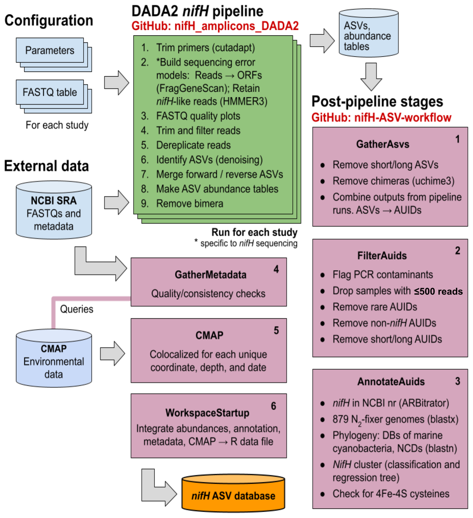
Figure 1 Schematic of the nifH amplicon data workflow. Data from all studies that met our criteria (Sect. 2.2) were downloaded from the NCBI (National Center for Biotechnology Information) Sequence Read Archive (SRA) and processed separately through the DADA2 nifH pipeline (green; Sect. 2.3.2), generally using identical parameters. ASV sequences and abundance tables from all studies were then combined and processed through each stage of the post-pipeline workflow (purple, Sect. 2.3.3) by executing the Makefile associated with each stage. Post-pipeline stages quality-filtered and then annotated the ASVs by reference to several nifH databases (DBs) and downloaded CMAP environmental data matched to the date, coordinates, and depth of each amplicon dataset. The main output of the entire workflow (pipeline and post-pipeline) is the nifH ASV database, which is available on Figshare (https://doi.org/10.6084/m9.figshare.23795943.v2; Morando et al., 2024b). The workflow is maintained in two GitHub repositories: one for the DADA2 nifH pipeline (https://github.com/jdmagasin/nifH_amplicons_DADA2; Morando et al., 2024a) and one for the post-pipeline stages (https://github.com/jdmagasin/nifH-ASV-workflow; Morando et al., 2024c).

Required inputs for the pipeline are raw nifH amplicon sequencing reads and sample collection metadata (at minimum the latitude and longitude, depth, and sample collection date and time) used to acquire environmental metadata from CMAP. Criteria for including publicly available datasets are detailed in Sect. 2.2.1.

The DADA2 software package is frequently used for processing 16/18S rRNA gene amplicon sequencing data due to its ability to remove base calling errors (“denoising”) and thereby infer error-free ASVs (Callahan et al., 2016). We have developed a customizable pipeline to improve the error models utilized by DADA2 by training them only on reads in a dataset that are valid nifH sequences (not PCR artifacts). The DADA2 pipeline runs from the command line in a Unix-like shell, moving through nine steps (Fig. 1, “DADA2 nifH pipeline”) described in Sect. 2.3.2 for each study independently. After the DADA2 pipeline is completed, outputs from all studies are integrated and refined by the six post-pipeline stages of the workflow, which perform additional quality filtering (e.g., size- and abundance-based selection), identify and remove spurious sequences (e.g., potential contaminants and non-target sequences), and annotate the ASVs (Fig. 1, “Post-pipeline stages”). By considering ASVs from all studies simultaneously, the workflow considers rare ASVs that might be discarded as irrelevant in a single-study analysis. Workflow stages are executed manually by running their associated Makefiles and Snakefiles within a Unix-like shell.

The workflow generates the final data product published in this work, the nifH ASV database, which includes ASV sequences, abundance and annotation tables, sample collection metadata, and sample environmental data from CMAP (Fig. 1). The database is available on Figshare (https://doi.org/10.6084/m9.figshare.23795943.v2; Morando et al., 2024b) as a set of tables (comma-separated value files) and an ASV FASTA file. However, these are also provided within an R data file, workspace.RData, in the WorkspaceStartup directory in the workflow GitHub repository for users who wish to analyze, curate, or customize the database using R packages for ecological analysis. All documentation, scripts, and data needed to run the workflow and produce the nifH ASV database are provided in the workflow GitHub repository (https://github.com/jdmagasin/nifH-ASV-workflow; Morando et al., 2024c). This includes pregenerated pipeline results for each of the 21 studies as well as the pipeline parameter files.

In summary, the workflow facilitates the systematic and reproducible exploration of nifH-based diversity within microbial communities and was applied to available nifH amplicon data to generate a globally distributed nifH ASV database. Together, the workflow and nifH ASV database will serve as valuable community resources, fostering future investigations while ensuring comparability between previous and forthcoming studies. In the following sections, detailed descriptions of each stage of the workflow are provided.

2.2 Compilation of nifH amplicon studies

2.2.1 Published studies

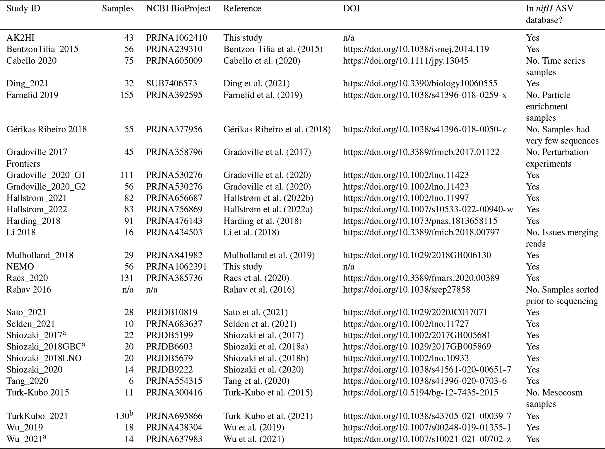
We compiled all publicly available nifH amplicon HTS data that were generated using the nifH1–4 primers (Zani et al., 2000; Zehr and McReynolds, 1989) and subsequently sequenced on the Illumina MiSeq/HiSeq platform, totaling 21 studies (Table 1). Limiting the scope to investigations that used the same amplification primers enabled a more tractable comparison across studies by different research groups that employed varying approaches to sample collection and preparation for sequencing by different centers. Datasets were downloaded from the National Center for Biotechnology Information (NCBI) Sequence Read Archive (SRA) using the GrabSeqs tool (Taylor et al., 2020) by specifying the study's NCBI project accession. Each dataset obtained included paired-end sequencing reads (in FASTQ files) and a table with the collection metadata for each sample. Some datasets could not be retrieved directly from the SRA and were obtained from the authors (Table A1). Note that we did not include studies where data were generated from experimental perturbations or particle enrichments (Table A1). Data were last accessed from NCBI SRA on 17 April 2024.

Table 1 Information on the studies compiled to generate the nifH ASV database. This includes the study ID used to refer to each dataset, the number of samples, NCBI BioProject accession, a reference to each publication, and its corresponding DOI.

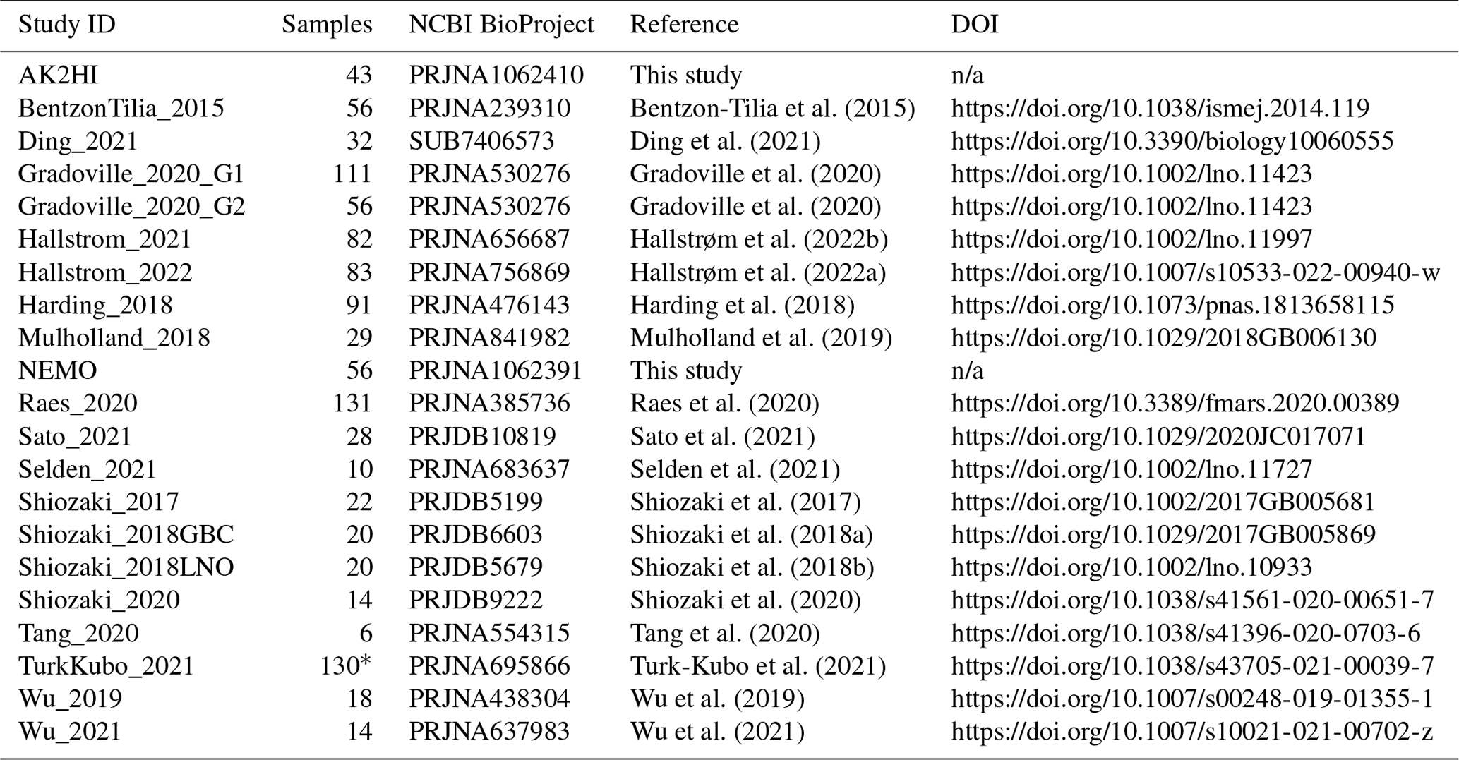
n/a: not applicable. ^∗ For TurkKubo_2021 only surface samples (n=59) are in the first release of the nifH ASV database.

Sample quality was validated prior to processing through the DADA2 nifH pipeline. Samples were discarded if they did not contain unmerged pairs of forward and reverse reads with properly oriented primer sequences (Table A1). There were two exceptions, studies by Shiozaki et al. (2017) and Shiozaki et al. (2018a), that used mixed-orientation sequence libraries and required preprocessing. The reads in each of these studies were partitioned by whether they captured the coding or template strand of nifH, determined by primer orientation. Because the quality of HTS reads generally degrades from 5^′ to 3^′, the partitioned data were run separately through the pipeline to preserve their sequencing error profiles for DADA2. The ASVs from the misoriented reads (e.g., forward reads with template sequence) were then reverse-complemented and combined with the properly oriented ASVs into a single ASV abundance table and FASTA file. Tables 1 and A1 provide information for obtaining the raw FASTQ files for all samples evaluated for the nifH ASV database including information regarding studies excluded from the database.

2.2.2 Unpublished nifH amplicon datasets

Additional nifH gene HTS datasets were included from DNA samples collected on two cruises in the North Pacific. One was a transect cruise across the eastern North Pacific (NEMO; R/V New Horizon, August 2014; Shilova et al., 2017) and the other was a transect cruise from Alaska to Hawaii (AK2HI; R/V Kilo Moana, September 2017). Euphotic zone samples were collected from Niskin bottles deployed on a CTD (conductivity–temperature–depth) rosette (NEMO) or from the underway water system (5 m; AK2HI). NEMO samples (2–4 L) were filtered through 0.2 and 3 µm pore-size filters (in series), while AK2HI samples (ca. 2 L) were filtered through 0.2 µm pore-size filters using gentle peristaltic pumping. Filters were dried, flash frozen, and stored at −80 °C until processing. DNA was extracted using a modified DNEasy Plant Mini Kit (Qiagen, Germantown, MD, USA) protocol, described in detail in Moisander et al. (2008), with on-column washing steps automated by a QIAcube (Qiagen).

Partial nifH DNA sequences were PCR amplified using the nifH1–4 primers in a nested nifH PCR assay (Zani et al., 2000; Zehr and McReynolds, 1989), according to details in Cabello et al. (2020). All samples were amplified in duplicate and pooled prior to sequencing. A targeted amplicon sequencing approach was used to create barcoded libraries as described in Green et al. (2015), using 5^′ common sequence linkers (Moonsamy et al., 2013) on second-round primers, nifH1 and nifH2. Sequence libraries were prepared at the DNA Service Facility at the University of Illinois at Chicago, and multiplexed amplicons were bidirectionally sequenced (2×300 bp, base pair) using the Illumina MiSeq platform at the W. M. Keck Center for Comparative and Functional Genomics at the University of Illinois at Urbana-Champaign. Samples were multiplexed to achieve ca. 40 000 high-quality paired reads per sample. The AK2HI and NEMO datasets can be found in the SRA (BioProject PRJNA1062410 and PRJNA1062391, respectively).

2.2.3 Sample collection data and co-localized CMAP environmental data

Sample collection data (e.g., coordinates, depth, date) and environmental data provide essential context for the interpretation of diazotroph omics datasets. Large-scale multivariate analyses depend on properly formatted, complete, and ideally quality-checked metadata from consistently collected and analyzed measurements. However, accessibility to this information is often limited (especially environmental data) for datasets published across multiple decades. Therefore, we first obtained sample collection metadata from the SRA and corrected or flagged errors and inconsistencies in the GatherMetadata stage of our post-pipeline workflow (described below) to ensure consistency and completeness. For each sample, the geographic coordinates, depth, and collection date (at local noon) from the SRA were used to query the Simons Collaborative Marine Atlas Project on 24 March 2023 (CMAP; https://simonscmap.com/; Ashkezari et al., 2021) for co-localized environmental data using a custom script (query_CMAP.py) in the CMAP stage of the workflow (Fig. 1). CMAP is an open-source data portal designed for retrieving, visualizing, and analyzing diverse ocean datasets, including research-cruise-based and autonomous measurements of biological, chemical, and physical properties; multi-decadal global satellite products; and output from global-scale biogeochemical models. For each sample, a mixture of 100 satellite-derived and modeled environmental variables from the CMAP repository were obtained. These, along with the SRA collection data, are included in our database. Aggregated metadata for all samples are summarized in Table S1 in the Supplement, but a detailed description of environmental metadata can be found at the CMAP website (https://simonscmap.com/catalog, last access: 21 January 2025). Metadata are available in the nifH ASV database (metaTab.csv for sample metadata and cmapTab.csv for environmental data).

2.3 Automated workflow for processing datasets with the DADA2 nifH pipeline

2.3.1 Installation of the DADA2 nifH pipeline and the post-pipeline workflow

The workflow (Fig. 1) comprises two software projects installed from separate GitHub repositories: nifH_amplicons_DADA2 which contains the ASV pipeline and ancillary scripts and nifH-ASV-workflow which integrates pipeline results for all datasets with annotation and CMAP environmental data to produce the data deliverable of the present work, i.e., the nifH ASV database. Installation requires cloning the nifH_amplicons_DADA2 repository (https://github.com/jdmagasin/nifH_amplicons_DADA2; Morando et al., 2024a) to a local machine and then downloading several external software packages using miniconda3. Detailed installation instructions are available from the GitHub web page, as well as a small tutorial to verify the installation on a small nifH amplicon dataset and introduce the two main pipeline commands (organizeFastqs.R and run_DADA2_pipeline.sh). Altogether, the installation and example take 30–40 min.

After installing the ASV pipeline, installation of the nifH-ASV-workflow proceeds similarly: clone the GitHub repository (https://github.com/jdmagasin/nifH-ASV-workflow; Morando et al., 2024c) and then download a few additional packages with miniconda3 (∼10 min to complete). For each study, the nifH-ASV-workflow includes the pipeline outputs (ASVs and abundance tables) which were used to create the nifH ASV database. Pipeline parameters and FASTQ input tables for each study are also provided for users who instead wish to rerun the pipeline starting from FASTQ files downloaded from the SRA. Because the nifH-ASV-workflow includes data and parameters specific to the studies used in this work, it has a separate GitHub repository from the pipeline. However, we emphasize that together they comprise the nifH amplicon workflow in Fig. 1.

Adding a new dataset to the workflow can be summarized in four steps. (1) Start a Unix-like shell that includes the required software (by “activating” a minconda3 environment called nifH_ASV_workflow). (2) Generate ASVs for the new dataset by running it through the pipeline, likely multiple times to tune parameters (Table 2). Output can be placed in the Data directory alongside other studies used in this work, and SRA metadata must be added to Data/StudyMetadata. (3) Include the new ASVs in the workflow by appending rows to the table GatherASVs/asvs.noChimera.fasta_table.tsv, which has file paths to all ASV abundance tables. (4) For each stage shown in Fig. 1, run the associated Makefile or Snakefile from the Unix-like shell by executing “make” or “snakemake -c1–use-conda”, respectively. Documentation resides within each Makefile or Snakefile. Input tables from the post-pipeline workflow also have embedded documentation.

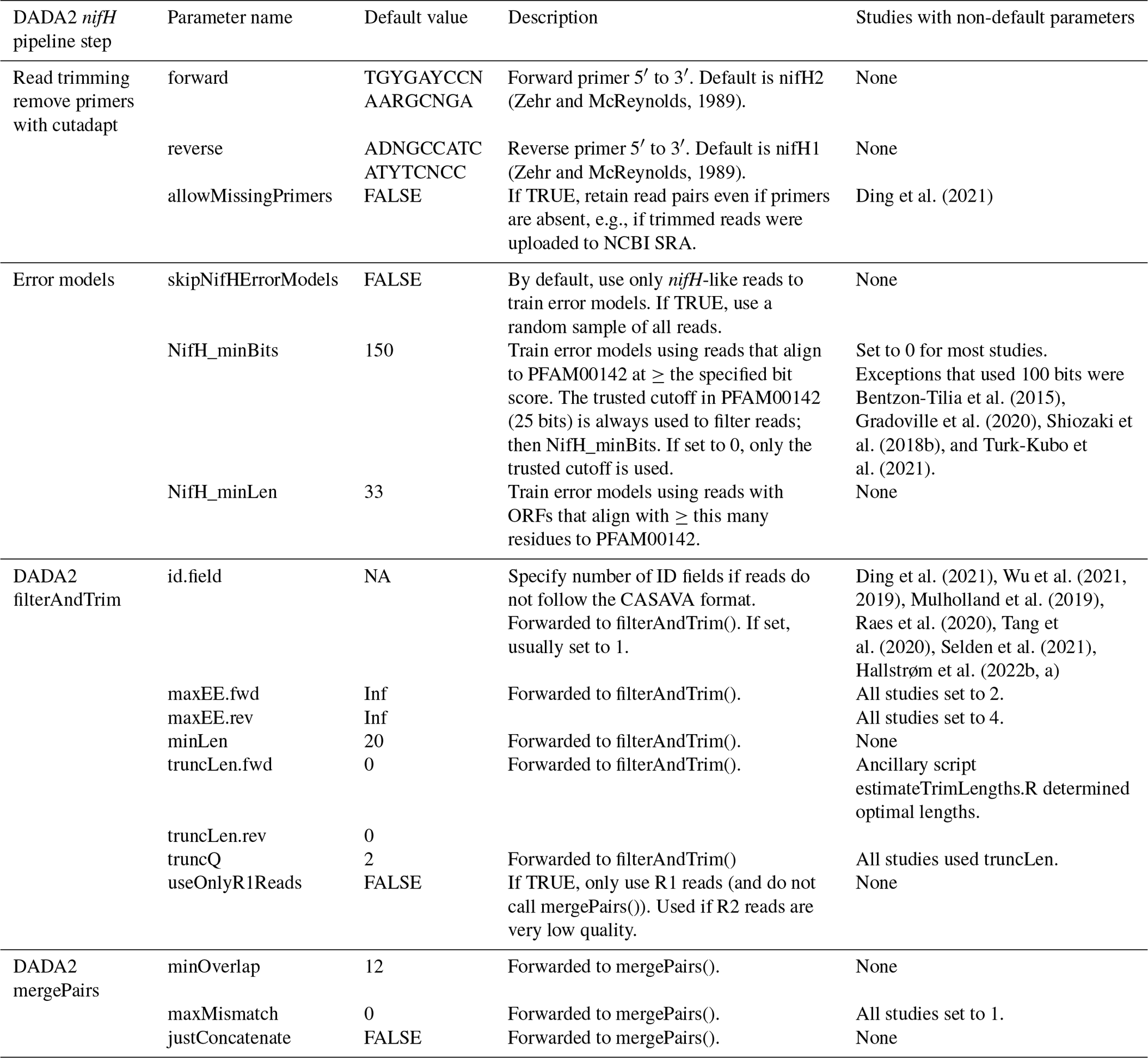
Table 2 Parameters for controlling the DADA2 nifH pipeline. Default values can be overridden in the text file that is passed to run_DADA2_pipeline.sh. Parameters for “Read trimming” and “Error models” are used in steps 1 and 2 of the pipeline (Fig. 1). The remaining parameters are important for controlling how DADA2 trims and quality filters the reads and merges forward and reverse sequences to create ASVs. The “Default value” column includes R constants for missing data (NA) and infinity (Inf).

2.3.2 DADA2 nifH pipeline

To encourage reproducible outputs and usage by non-programmers, the DADA2 pipeline (GitHub repository: nifH_amplicons_DADA2) is controlled by a plain text parameter file (Table 2) and a descriptive table of input samples (the “FASTQ map”). Since a study might include samples with vastly different diazotroph communities and relative abundances, potentially impacting ASV inferences by DADA2, the FASTQ map for a study enables samples to be partitioned into “processing groups” that are each run separately through DADA2. For example, in the present work processing groups usually partitioned the samples in a study by the unique combinations of collection station or date, nucleic acid type (DNA or RNA), size fraction, and collection depth. Pipeline outputs for each processing group are stored in a directory hierarchy with levels that follow the processing group definition. Partitioning datasets into processing groups greatly improves the overall speed of DADA2 and simplifies subsequent analyses that compare ASVs detected in different kinds of samples (e.g., detected versus transcriptionally active diazotrophs or presence across different stations, depths, and/or size fractions). For generating the nifH ASV database, studies that met selection criteria (Sect. 2.2.1 and Table 1) were run through the pipeline using the study-specific FASTQ maps and parameters available in the Data directory of the nifH-ASV-workflow GitHub repository.

The DADA2 pipeline runs from the command line in a Unix-like shell, moving through nine main steps (Fig. 1, DADA2 nifH pipeline): (1) trim reads of primers using cutadapt (Martin, 2011), (2) build sequencing error models, (3) make FASTQ quality plots, (4) trim and filter reads based on quality, (5) dereplicate, (6) denoise (ASV inference), (7) merge forward and reverse sequences, (8) make the ASV abundance table, and (9) remove bimera (see Callahan et al., 2016, for steps 2 through 9). These steps will be familiar to DADA2 users, except that for step 2 the error models are only trained on nifH-like reads (discussed below). To run the pipeline on other functional genes, the parameter file would need to be edited to disable nifH-based error models and to include the expected primers. We again note that the DADA2 pipeline is distinct from the post-pipeline workflow stages which are specific to this work, but together they comprise the workflow in Fig. 1.

DADA2 parameters impact the ASV sequences identified and the number of reads used. Thus, exploring parameters is essential for checking the robustness of ASVs (particularly rare ones) and their relative abundances. The method and parameters used to trim the reads are especially important because most pipeline steps occur after filterAndTrim (Fig. 1). Two methods are supported: one can trim each read based on its quality degradation (truncQ parameter to the DADA2 filterAndTrim function; Table 2) or all reads at the same position determined by inspecting sample FASTQ quality plots (truncLen parameter; Table 2, and comparison of methods in Appendix B). The latter approach can be labor-intensive and unsystematic for studies with tens to hundreds of samples. To address this, the ancillary script estimateTrimLengths.R can be used to determine trimming lengths that will maximize the percentage of reads that make it through the pipeline. For each FASTQ file in a study, the script chooses 1000 read pairs at random and removes the primers. Then the read pairs are trimmed using every combination of lengths over a window (from 55 %–85 % of the median read length in 15 bp steps), and successful merges (with ≥12 bp overlapping and ≤2 mismatches) are counted. The counts are averaged across all samples (weighting by sequencing depths), and the top 10 combinations of forward and reverse trimming lengths are reported in a table, with estimates for the percentages of reads retained and the mean errors per read to help choose the maxEE parameters (Table 2).

The pipeline allows one to rerun DADA2 steps 3–9, with outputs saved in separate, date-stamped directories. Primer removal and error models (steps 1–2) are unlikely to benefit much from parameter tuning, so the pipeline reuses outputs from those steps. Log files and diagnostic plots created by the pipeline are intended to facilitate parameter evaluation as well as to capture statistics to support publication. Moreover, logs and other pipeline outputs are consistently formatted across pipeline runs, which enables scripts to aggregate and analyze results across datasets such as in our workflow.

Step 1 only consisted of primer removal using cutadapt (Martin, 2011). Raw reads were retained only if the forward (nifH2) and reverse (nifH1) primers were both found on the R1 and R2 reads, respectively. DADA2 sequencing error models were built at step 2 using only the reads predicted to be nifH rather than a subsample of all reads as in typical use of DADA2. Reads likely to encode nifH were identified as follows: FragGeneScan (version 1.31; Rho et al., 2010) was used to predict open reading frames (ORFs) on R1 reads which were then aligned to the nitrogenase Pfam (Mistry et al., 2021) model (PF00142.20) using HMMer3 (hmmsearch version 3.3.2; http://hmmer.org, last access: 21 January 2025). ORFs with >33 residues and a bit score that exceeded the trusted cutoff encoded in the model (25.0 bits) were retained. Prefiltering the reads aims to reduce the effects of PCR artifacts on the error models. For some studies, this approach resulted in increases (∼3 %–10 %) in the total percentage of reads retained in ASVs and fewer total ASVs compared to using error models based on a subsample of all reads. Adapting the pipeline to a different marker gene would only require substituting an appropriate Pfam model or disabling step 2 (by setting skipNifHErrorModels to TRUE; Table 2), which forces the pipeline to make error models by subsampling from all reads. At step 4, DADA2 filterAndTrim() trimmed forward and reverse reads using the lengths suggested by estimateTrimLengths.R and then discarded read pairs that had excessive errors (>2 for R1 reads, >4 for R2 reads) or were <20 bp. Conservative parameters were used for merging sequences: at most 1 bp was allowed to mismatch in the forward and reverse sequence overlap of minimally 12 bp (stage 7). Dereplicating (step 5), denoising, ASV calling (step 6), generating an abundance table (step 8), and bimera detection (step 9) were all performed with default DADA2 parameters. Datasets that passed preprocessing steps (Table 1) were run through the DADA2 pipeline using mostly identical parameters, except for the trimming lengths (truncLen.fwd and truncLen.rev in Table 2).

2.3.3 Post-pipeline stages

The workflow post-pipeline stages (GitHub repository: nifH-ASV-workflow) combine the pipeline outputs, conduct further quality control steps, co-locate the samples with environmental data from the CMAP data portal, and annotate the ASVs (Fig. 1, Post-pipeline stages). Key outputs from the post-pipeline are the following: a unified FASTA with all the unique ASVs detected across all the studies (i.e., all samples), tables of ASV total counts and relative abundances in all studies, multiple annotations for each ASV by comparison to several nifH reference databases, and CMAP environmental data for each sample. These outputs comprise the nifH ASV database and are all available within an R image file (workspace.RData) generated by the workflow which is included in the nifH-ASV-workflow repository. Provision as an R image will make the outputs immediately accessible to many researchers who prefer R due to its extensive packages for ecological analysis. The nifH ASV database is also available on Figshare (https://doi.org/10.6084/m9.figshare.23795943.v2; Morando et al., 2024b). The remainder of this section describes each of the post-pipeline stages.

The GatherAsvs stage aggregated ASV sequences and abundances across all DADA2 pipeline runs (i.e., from all samples and studies). First, ASVs were filtered based on length. Chimera sequences were then removed using UCHIME3 denovo (Edgar, 2016a) via VSEARCH (Rognes et al., 2016). Chimera sequences were identified within each sample, but the final classification was based on majority vote (chimera or not) across the samples in the processing group. Second, the GatherAsvs stage combined the non-chimeric ASVs from all studies into a single abundance table and FASTA file. Since each study is run independently through the DADA2 pipeline, ASV identifiers are not consistent across studies. Therefore, each unique ASV sequence was renamed with a new unique identifier of the form AUID.i, where AUID stands for ASV Universal IDentifier. The scripts used to rename the ASVs (assignAUIDs2ASVs.R) and to create the new abundance table (makeAUIDCountTable.R) are available at the nifH_amplicons_DADA2 GitHub repository (in scripts.ancillary/ASVs_to_AUIDs). The script assignAUIDs2ASVs.R optionally takes an AUID reference FASTA so that AUIDs can be preserved as new datasets are added to future versions of the nifH ASV database.

Both rare and potential non-nifH sequences were assessed on the unified AUID tables in the next stage, FilterAuids (Fig. 1). First, possible contaminants were identified by the Makefile invocation of check_nifH_contaminants.sh, provided as an ancillary script in the pipeline GitHub repository. In brief, check_nifH_contaminants.sh first translated all ASVs into amino acid sequences using FragGeneScan (Rho et al., 2010), which were then compared using blastp to 26 contaminants known from previous nifH amplicon studies (Zehr et al., 2003; Goto et al., 2005; Farnelid et al., 2009; Turk et al., 2011). ASVs that aligned at >96 % amino acid identity to known contaminants were flagged. Next FilterAuids removed samples with ≤500 reads and rare ASVs, defined as those that did not have at least 1 read in at least two samples or ≥1000 reads in one sample.

Next, the ancillary script, classifyNifH.sh, was employed to identify and remove non-nifH-like sequences. The script utilized blastx to search each ASV against ∼44 000 positive and ∼15 000 negative examples of NifH protein sequences that were found in NCBI GenBank by ARBitrator (run on 28 April 2020; Heller et al., 2014). ASVs were classified based on the relative quality of their best hits in the two databases, similar to the “superiority” check in ARBitrator. An ASV was classified as positive if the E value of its best positive hit was ≥10 times smaller than the E value for the best negative hit, and vice versa for negative classifications. ASVs failing to meet these criteria were classified as “uncertain”. The blastx searches used the same effective sizes for the two databases (-dbsize 1 000 000), so that E values could be compared, and retained up to 10 hits (-max_target_seqs 10).

The FilterAuids stage of the workflow exclusively discarded ASVs with negative classifications. “Uncertain” ASVs were retained as potential nifH sequences not in GenBank. In the last stage, FilterAuids excluded ASVs with lengths that fell outside 281–359 nucleotides, a size range which in our experience encompasses the majority of valid nifH amplicon sequences generated by nested PCR with nifH1–4 primers.

For each AUID in the nifH ASV database, we provide taxonomical annotations using several different approaches, encompassed by the AnnotateAuids stage (Fig. 1) and accessible through ancillary scripts in the GitHub repository (in scripts.ancillary/Annotation). The script blastxGenome879.sh enables a protein-level comparison via blastx against a database of 879 sequenced diazotroph genomes (“genome879”, https://www.jzehrlab.com/nifh, last access: 21 January 2025). Here, the closest cultivated relative for each AUID was determined by the smallest E value among alignments with ≥50 % amino acid identity and ≥90 % query sequence coverage. Cautious interpretation is suggested, because the reference database is small and contains only cultivable taxa. Similarly, the top nucleotide match of each AUID was identified by an E value within alignments possessing ≥70 % nucleotide identity and ≥90 % query sequence coverage obtained by blastn against a curated database of nifH sequences (July 2017 nifH database, https://www.jzehrlab.com/nifh) by executing the blastnARB2017.sh script. Additionally, nifH cluster annotations were assigned to each ASV using the classification and regression tree (CART) method of Frank et al. (2016). This approach was implemented as part of a custom tool that predicted ORFs for the ASVs with FragGeneScan, then performed a multiple sequence alignment on the ORFs, and then applied the CART classifier. The tool is available as the ancillary script: assignNifHclustersToNuclSeqs.sh.

The Makefile created and searched against two “phylotype” databases, one containing 223 nifH sequences from prominent marine diazotrophs including NCDs (Turk-Kubo et al., 2022) and another with 44 UCYN-A nifH oligotype sequences (Turk-Kubo et al., 2017). These databases were searched using blastn with the effective database size of the ARB2017 database (-dbsize set to ∼29 million bases) to enable E-value comparisons across all three searches. For each ASV, we provide phylotype annotations based on the top hit by E value if the alignment had ≥97 % nucleotide identity and covered ≥70 % of the ASV. Finally, ORFs for all ASVs were searched for highly conserved residues which are thought to coordinate the 4Fe-4S cluster in NifH, specifically for paired cysteines shortly followed by alanine, methionine, and proline residues (AMP; described in Schlessman et al., 1998). This simple check, performed by the script check_CCAMP.R, was intended to complement the reference-based annotations above. The presence of cysteines and AMP could be used to retain ASVs that have no close reference. Absence could be used to flag ASVs that, despite high similarity to a reference sequence, might not represent functional nifH (e.g., due to frame shifts).

Since the annotation scripts provided multiple taxonomic identifications for most of the AUIDs, a primary taxonomic ID was assigned for each AUID using the script make_primary_taxon_id.py. If a phylotype annotation (e.g., Gamma A) was assigned, this became the primary taxonomic ID; otherwise, cultivated diazotrophs from genome879 were used (e.g., Pseudomonas stutzeri). Finally, when neither a phylotype nor a cultivated diazotroph could be determined, the nifH cluster (e.g., “unknown 1G”) was used. AUIDs without an assigned nifH cluster or taxonomic rank below domain were removed from the final nifH ASV database unless paired cysteines and AMP were detected. This final data filtration step occurred in the WorkspaceStartup stage described below.

The CMAP stage was managed by a Snakefile that called the script query_cmap.py to query the CMAP data portal for co-localized environmental data (Fig. 1). The script was given the main output from the GatherMetadata stage, metadata.cmap.tsv, which is a table of the collection coordinates, dates at local noon, and depths from all the samples. GatherMetadata reported any samples with missing metadata and ensured standardized formats for the required query fields. Additionally, query_cmap.py validated fields prior to querying CMAP. It should be noted that the precision of values obtained from CMAP depend on floating-point arithmetic and not the significant digits of the underlying measurement or model. Therefore, prior to an analysis requiring high precision for specific CMAP variables, it is recommended to consult the original producer of the data to determine the significant digits.

The last stage of the workflow, WorkspaceStartup, filtered out AUIDs that had no annotation and then generated the final nifH ASV database, which is comprised of AUID abundance tables (counts and relative), AUID annotations, sample metadata, and corresponding environmental data. These data are provided as text files (.csv and FASTA) within a single compressed file (.tgz) that is available on Figshare (https://doi.org/10.6084/m9.figshare.23795943.v2; Morando et al., 2024b) as well as within the workflow GitHub repository within an R image file (workspace.RData).

2.4 Diazotroph biogeography from a DNA dataset of the nifH ASV database

The DNA dataset, a custom version of the nifH ASV database restricted to DNA samples (representing a majority of the database, only removing 108 cDNA samples out of 944 total samples), was created to showcase the utility of the workflow. Additional data reduction steps were conducted, averaging replicates and samples from the same location but different size fractions, to enable comparisons between different sampling methodologies.

3 Results and discussion

3.1 Generation of the marine nifH ASV database

All publicly available marine nifH amplicon HTS data from studies that met our criteria, including two new studies, were compiled in the present investigation (see Sect. 2.2 and Table A1). Altogether 982 samples from 21 studies, comprising a total of 87.7 million reads (Table 3), were processed through the entire workflow, i.e., the DADA2 nifH pipeline (Sect. 2.2.2) as well as the post-pipeline stages (Sect. 2.2.3). The nifH ASV database, i.e., the ASV sequences, abundances, and annotations, as well as sample collection and CMAP environmental data, was generated from the 944 samples, 9383 ASVs, and 43.0 million reads that were retained by this workflow (Figs. 1 and 2 and Table 3). To our knowledge, it is the only global database for marine diazotrophs detected using nifH HTS amplicon sequencing, with comprehensive and standardized ancillary data (Fig. 2 and Table S1).

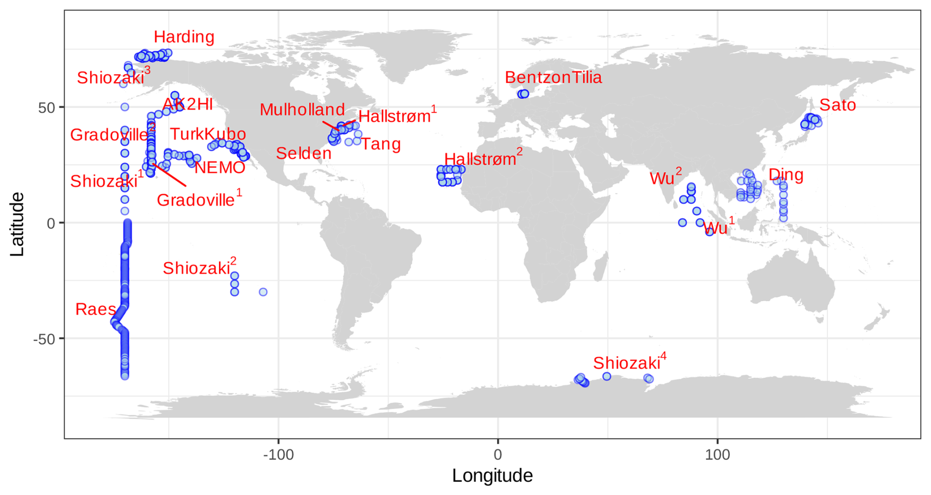
Figure 2 Global sampling distribution of the nifH ASV database. World map of sampling locations for the datasets compiled and processed to construct the nifH ASV database. Abbreviated study IDs are used with superscripts ordered by publication year for Shiozaki (2017, 2018a, b, and 2020), Hallstrøm (2021 and 2022), and Wu (2019 and 2021). For Gradoville, the superscripts indicate Gradients cruises 1 and 2. See Table 1 for the citation source linked to each study ID.

Table 3 Summary of the full nifH workflow. The table shows the number of samples, ASVs, and reads retained through the entire workflow (the DADA2 nifH pipeline and major post-pipeline stages) to create the nifH ASV database. The vast majority of ASVs that were removed by GatherAsvs fell outside 200–450 nt. WorkspaceStartup removed ASVs with no annotation and samples that had zero reads after ASV filtering.

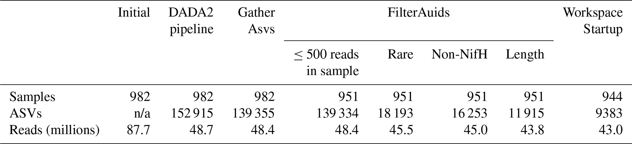
n/a: not applicable

Interestingly, studies were affected differently by each step of the DADA2 nifH pipeline (Fig. 3 and Table 4). There were major losses of reads during ASV merging, with several studies retaining <40 % of their total reads by the end of the pipeline (i.e., Hallstrom_2022, Sato_2021, and Shiozaki_2020), though on average about 60 % of the reads were retained across studies (Fig. 3 and Table 4).

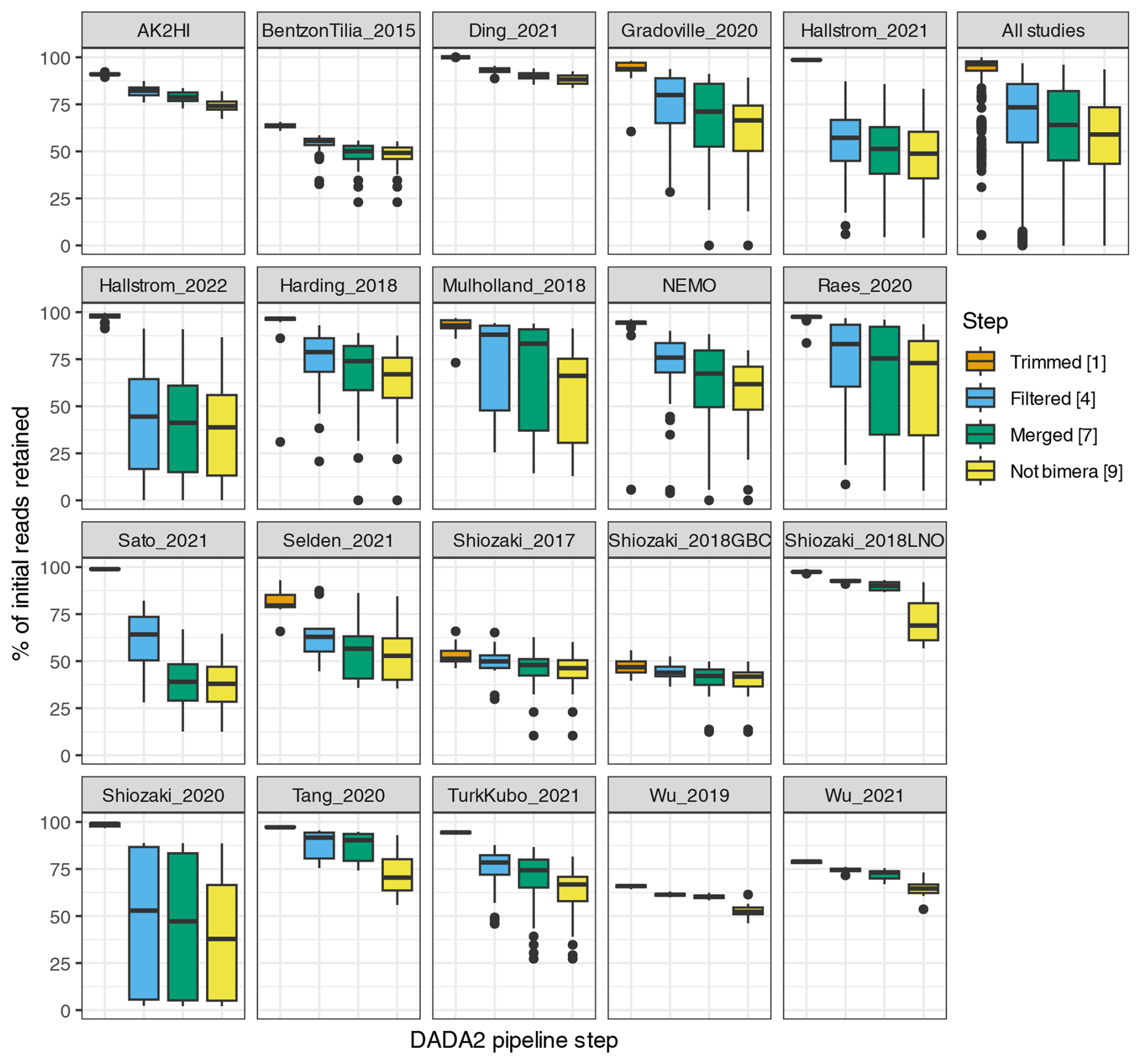
Figure 3 Study-specific retention of reads at each stage of the pipeline. The proportion of total reads in each sample that are retained at the completion of each step of the DADA2 nifH pipeline is shown. Each box shows the distribution for samples in the indicated study (using study IDs in Table 1) or for all samples together (top right). Proportions for Shiozaki_2017 and Shiozaki_2018GBC reflect that approximately half the amplicons were not in the orientation expected by the pipeline (see text). Numbers in the legend indicate pipeline steps in Fig. 1.

Table 4 Quality filtering by the DADA2 nifH pipeline. For each study, the mean numbers of reads retained per sample at the end of each stage of the DADA2 nifH pipeline, as well as the mean percentage of reads retained, are shown. Statistics in the bottom three rows pool all samples. “Initial”, “Trimmed⁴”, “Filtered⁴”, “Merged⁷”, and “Non-bimera⁹” with their superscripts are specific to the pipeline steps in Fig. 1. At each step (column), the calculations only include the samples that have more than zero reads.

Post-pipeline stages of the workflow further refined the data (detailed in Methods) (Fig. 4). First, GatherAsvs identified and removed 163 chimeras using uchime3 denovo (distinct from the bimera filtering done by the pipeline), and then removed ∼8700 ASVs that were far outside expected nifH lengths (200–450 nt). AUIDs were assigned to the remaining ∼139 000 unique non-chimeric ASVs (comprising 48.4 million total reads; Tables 3 and 5). The FilterAuids stage had the largest impacts on retained data. Thirty-one samples with ≤500 reads were removed because they would likely misrepresent their diazotrophic communities. The FilterAuids rarity check had the greatest reduction to pipeline outputs (∼121 000 ASVs removed and 6.0 % of reads), followed by the length filter (∼4000 ASVs and 2.7 % of reads; Tables 3 and 5).

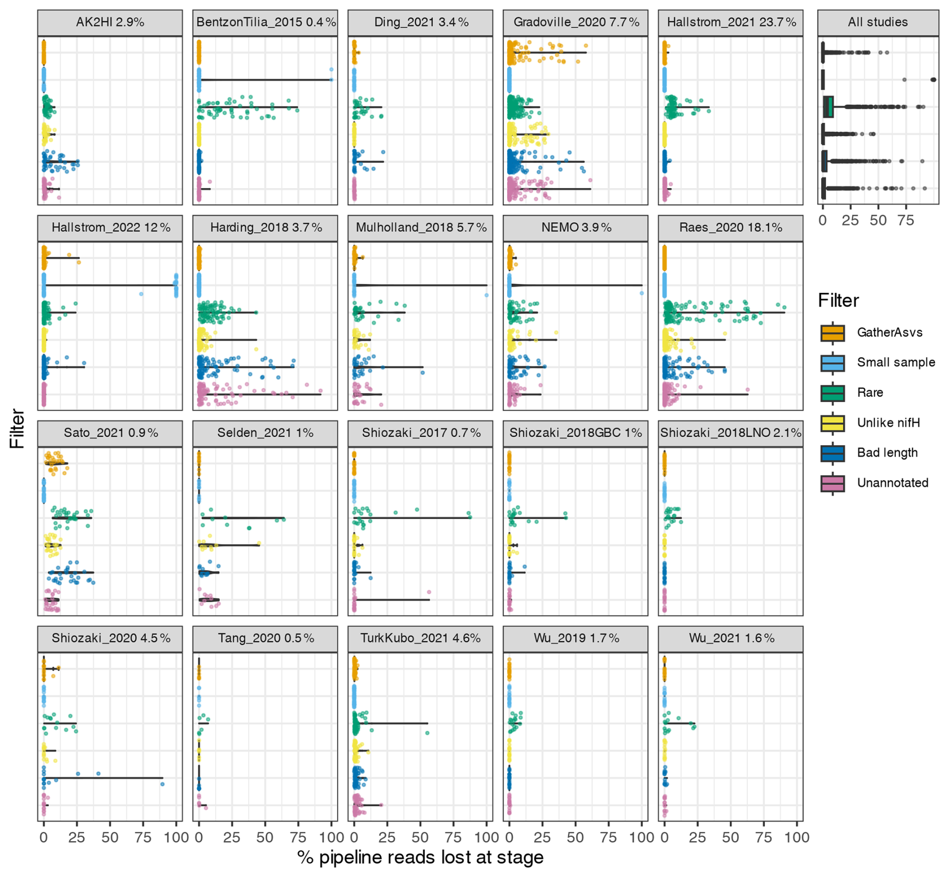
Figure 4 Study-specific loss of reads at each stage of the post-pipeline workflow. For each study, the violin plots show how many reads from the pipeline were removed by GatherAsvs due to length, the four filtering steps of FilterAuids, or WorkspaceStartup due to the ASV having no annotation (shown in Fig. 1). Losses for all samples combined are shown in the box plot (top right). Bracketed numbers after each study ID indicate the percentage of reads that contributed to the nifH ASV database, e.g., 23.7 % of all the reads in the database were from Hallstrom_2021.

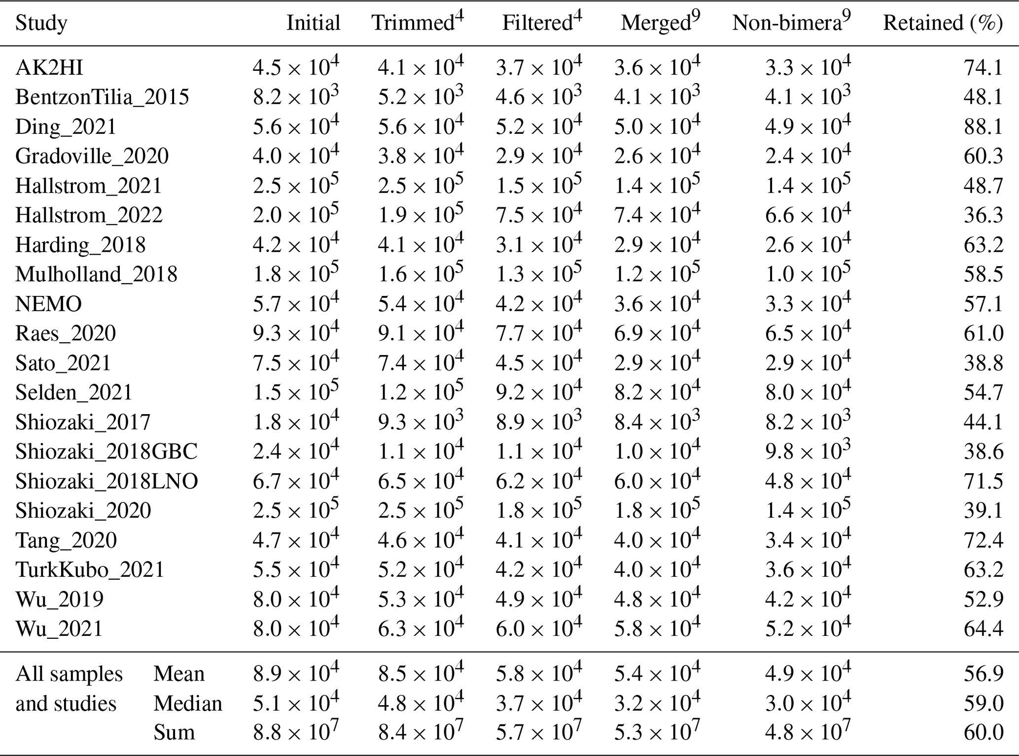
Table 5 Quality filtering by the post-pipeline workflow. For each study, the mean numbers of reads per sample that were output by the DADA2 nifH pipeline and retained by the GatherAsvs, FilterAuids, and WorkspaceStartup stages of the post-pipeline workflow are shown. The “Retained (%)” column has the mean percentages of reads retained per sample (relative to column “DADA2 pipeline” values). Additionally, the last three rows show the overall means, medians, and sums of reads across all samples and studies. Superscripts correspond to stage numbers in Fig. 1, “Post-pipeline stages”. The “GatherAsvs¹” column mainly reflects length filtering (200–450 nt), and the “WorkspaceStartup⁶” column reflects discarding of ASVs that had no annotation. At each stage (column), the calculations include only the samples that have more than zero reads.

Finally, ASVs were removed if they were classified as non-nifH, based on a strong alignment to sequences in NCBI GenBank that ARBitrator (Heller et al., 2014) classified as non-nifH. Specifically, an ASV was classified as non-nifH if the ratio of E values for its best positive and negative hits, among sequences classified by ARBitrator, was >10. A total of 137 366 of the 139 355 non-chimera ASVs had database hits which resulted in 50 233 positive, 20 528 negative, and 66 605 uncertain classifications. This approach was used to leverage ARBitrator's high specificity for detecting nifH as well as to enable users to identify ASVs that have high percent identity matches to sequences in GenBank. An alternative approach would have been to classify the ASVs based on their alignments to HMMs (hidden Markov models) for NifH versus NifH-like proteins (e.g., protochlorophyllide reductase), used by the NifMAP pipeline for nifH operational taxonomic units (Angel et al., 2018). Finally, FilterAuids removed ASVs with lengths outside 281–359 nt, a total of 4338 ASVs comprising 1.2 million reads (Figs. 1 and 4 and Tables 3 and 5). After FilterAuids, the total number of samples in the dataset was reduced from 982 to 951, and the number of ASVs was reduced from 139 355 to 11 915.

FilterAuids also flagged a total of 2342 ASVs as possible PCR contaminants. Although we opted to flag, not remove, these ASVs, the workflow can be easily altered to remove contaminants. Most studies contained low levels of contamination (≤1 %) based on our criteria. However, several studies were flagged with ∼9 %–29 % of their reads being similar to known contaminants. Identifying potential contaminants is challenging given their numerous sources, study-specific nature (Zehr et al., 2003), and lack of control sequence data from blanks.

Next, AnnotateAuids assigned annotations using our three nifH reference databases and CART (Fig. 1). In total, 9406 of the 11 915 quality-filtered ASVs were annotated, usually with multiple references (Fig. A1). Most (9322 ASVs) had hits to both genome879 and ARB2017, likely because the 879 sequenced diazotrophs had nifH homologs in GenBank that were found by ARBitrator. Fewer ASVs had hits to the databases that targeted UCYN-A oligonucleotide sequences (217 ASVs) and other marine diazotrophs (938 ASVs; 211 ASVs also had UCYN-A hits). Most ASVs (9380 total) were assigned to NifH clusters 1–4 by CART (respectively 4923, 101, 4205, and 151 ASVs), including five ASVs that had no hits for our databases. The majority of ASVs (9257 total) had open reading frames (ORFs) that contained paired cysteines and AMP which might coordinate the 4Fe-4S cluster, and all 9257 also had annotation from the reference databases or CART. A few ASVs had annotations but lacked residues to coordinate 4Fe-4S: 29 ORFs lacked the paired cysteines, and another 120 ORFs had paired cysteines but no AMP, usually due to a substitution for M. The last step of AnnotateAuids assigned primary IDs (described above) to 9383 ASVs. All of them were retained in the final stage of the post-pipeline workflow, WorkspaceStartup (below).

In the CMAP stage, sample collection metadata (date, latitude, longitude, and depth) were used to download CMAP environmental data (100 variables) for each sample in the nifH ASV database (Fig. 1). The CMAP data will enable analyses of potential factors that influence the global distribution of the diazotrophic community. Aggregated metadata for all samples are available in the nifH ASV database (metaTab.csv for sample metadata and cmapTab.csv for environmental data).

The last stage of the post-pipeline workflow is WorkspaceStartup, which generates the nifH ASV database (Fig. 1). ASVs with no annotation are removed as well as samples with zero total reads due to ASV filtering steps. The nifH ASV database consisted of 21 studies, 944 samples, 9383 ASVs, and 43.0 million total reads (Tables 3 and 5). The database is heavily biased toward euphotic zone DNA samples, with euphotic heuristically defined as follows. Samples were classified as coastal (<200 km from a major landmass) or open ocean. Euphotic samples were then identified as those collected above a depth cutoff, 50 m for coastal samples and 100 m for open ocean. Samples obtained from DNA (n=836) far exceeded those from RNA (n=108) extracts. Likewise, a majority of the samples were from the euphotic zone (861 compared to 83 from the aphotic zone). The database also includes replicate samples (n=286) and size-fractionated samples (n=170).

3.2 Global nifH ASV database

3.2.1 Comparison to an operational taxonomic unit database

New studies with Illumina amplicon data have mainly used DADA2 (Callahan et al., 2016) and other methods that distinguish fine-scale variation from sequencing errors (Eren et al., 2014; Edgar, 2016b; Amir et al., 2017). Earlier studies, including 13 of the 19 previously published studies in the nifH ASV database (Table C1), used de novo operational taxonomic units (OTUs) which were obtained by clustering the sequences at 97 % nucleotide identity. OTUs masked sequencing errors as well as fine-scale variation and had other disadvantages compared to ASV approaches (Callahan et al., 2017). Although cross-study comparisons ideally will use the same pipeline for all the studies (the motivation for our workflow), previously published results should be considered. Therefore, for each study in the nifH ASV database, diazotroph communities were compared to versions generated using the NifMAP OTU pipeline (Appendix C). The ASV and OTU communities mainly had similar nifH clusters, except for several studies where the workflow retained substantially more sequencing reads (Fig. C1, Table C1).

3.2.2 Sample distribution

Investigations of N₂ fixation and diazotrophic communities have focused on specific ocean regions, and this is reflected by the uneven global distribution of nifH amplicon datasets in the nifH ASV database (Figs. 2, 5a and b). There is an outsized influence of the Northern Hemisphere, especially in the Pacific Ocean where most of the database samples were located (439), and 68.3 % of these samples originated from the Northern Hemisphere (Figs. 2, 5a and b, and 6). Ten studies are found within the Pacific, with several containing >50 samples (Figs. 2 and 6). Notably, Raes_2020 (Raes et al., 2020) is the largest dataset stretching from the Equator to the Southern Ocean, making up almost the entirety of the Southern Hemisphere Pacific samples (Figs. 2 and 6). Two new studies carried out in the North Pacific constitute the only previously unpublished data of the nifH ASV database (Table 1). AK2HI was a latitudinal transect from Alaska (USA) to Hawaii (USA), and NEMO was a longitudinal transect across the eastern North Pacific from San Diego, CA (USA), to Hawaii (USA) (Fig. 2; Sect. 2.2.2). The amplicon data compiled for the nifH ASV database were primarily generated from DNA, with most RNA samples deriving from Atlantic Ocean studies and no contribution from RNA samples in the Arctic or Indian oceans (Fig. 6).

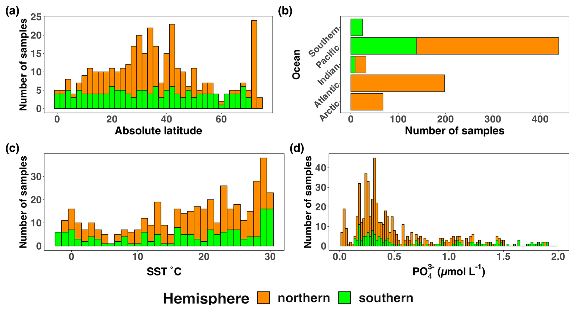
Figure 5 Location, temperature, and phosphate distributions of the nifH ASV database. The number of samples from the nifH ASV database by (a) absolute latitude, (b) the world's oceans, (c) sea surface temperature (SST, °C), and (d) Pisces-derived ${{\mathrm{PO}}_{\mathrm{4}}}^{\mathrm{3}-}$ (µmol L⁻¹). Environmental data, (c) and (d), were retrieved from the CMAP data portal. All bars are stacked.

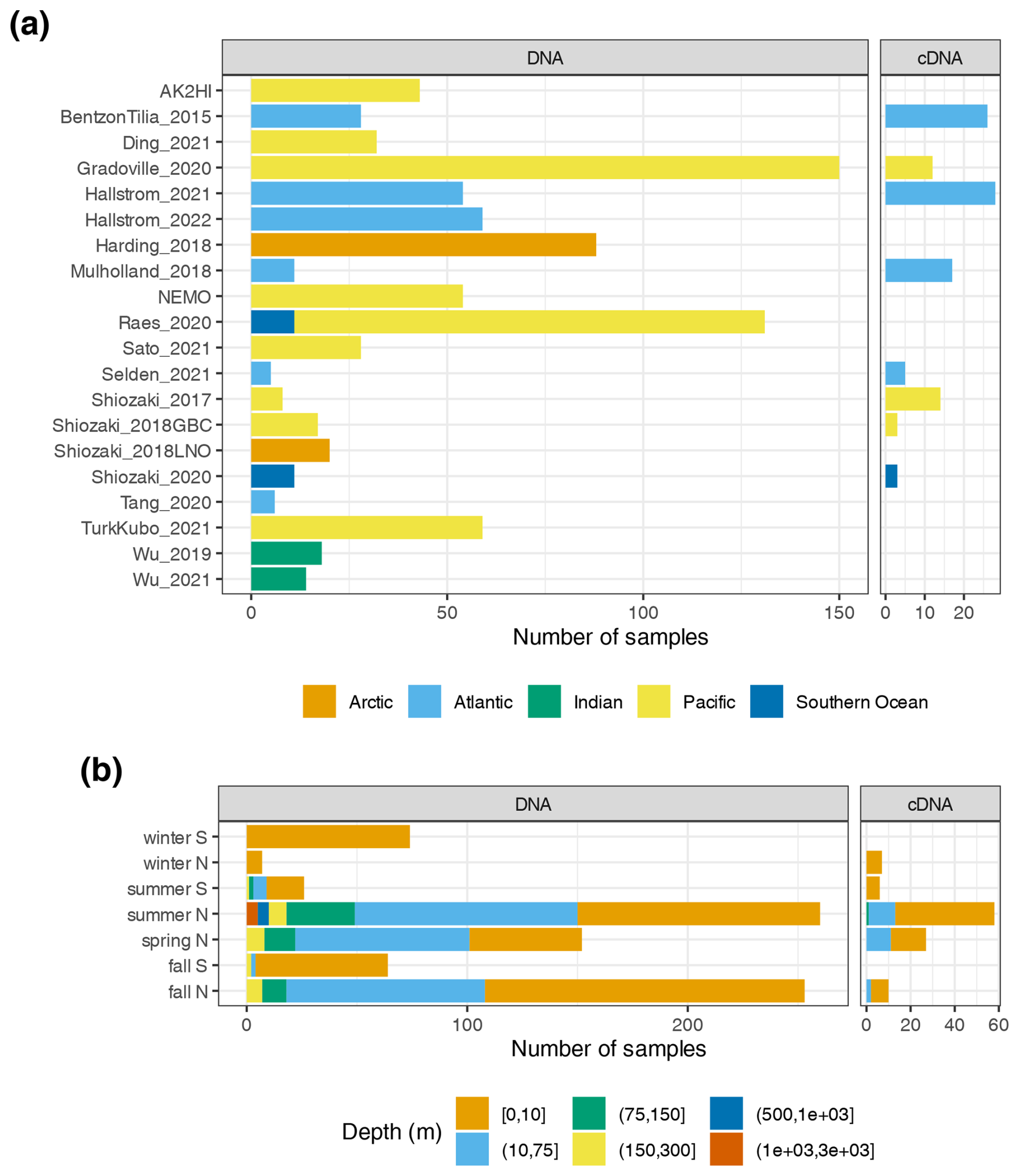
Figure 6 Samples in the nifH ASV database by collection location, season, and amplicon type. The numbers of samples from each study are shown by ocean and study (a), as well as by the collection season, hemisphere, and depth (b). For both panels, the amplicon type (DNA or cDNA) is shown, but x axis scales differ between (a) and (b). See Table 1 for citations for the studies in (a).

Undersampled regions include the eastern South Pacific (n=6) and the western Indian Ocean (n=0) (Figs. 2, 5a, and 6a). Only two studies originated from the Indian Ocean, a unique environment with intense weather and shifting circulation patterns that include monsoon seasons and upwelling conditions, that will require much greater sampling coverage to capture diazotroph biogeography. No South Atlantic samples were found during compilation that met the criteria for inclusion in the nifH ASV database, though there are several studies from this region (Table A1). Most Atlantic Ocean samples were coastal and from the North Atlantic. Thus, the Atlantic subtropical gyres, which are known to host diverse diazotrophs (Langlois et al., 2005), are underrepresented by nifH amplicon data (Fig. 2).

Tropical and subtropical regions, often associated with high temperatures and low nutrients, are highly represented in the database (Figs. 2 and 5a). This likely influenced the ranges of environmental variables with most samples in the database originating from locations with SST above 15 °C and ${{\mathrm{PO}}_{\mathrm{4}}}^{\mathrm{3}-}$ below 0.5 µmol L⁻¹ (Figs. 5c and d). Northern Hemisphere samples were collected in all seasons, though fewer from the winter. In contrast, most Southern Hemisphere samples were collected in the winter and fall (Fig. 6b). While most DNA samples are from the euphotic zone (Fig. 6b), cDNA samples are almost exclusively from the euphotic zone and mainly from the Northern Hemisphere during the spring and summer (Fig. 6b), indicating an incomplete picture of diazotroph activity.

The disproportionate spatial and seasonal coverage between hemispheres in the nifH ASV database mirrors collection biases in other N₂ fixation metrics: N₂ fixation rate measurements; diazotroph cell counts; and nifH qPCR data, which are heavily sourced from the North Atlantic (Shao et al., 2023) or, when targeting NCDs, also the North Pacific (Turk-Kubo et al., 2022). These biases underscore the need for future work in understudied regions and seasons.

3.3 Global diazotroph assemblages of the DNA dataset

3.3.1 Clusters 1B and 1G were dominant in most studies

To demonstrate how the nifH ASV database can be used, a subset of the data was created that comprised all DNA samples (88.8 % of the total dataset; Fig. 7) and is referred to herein as the “DNA dataset.” Samples derived from cDNA (n=108; Fig. 6) were removed. Replicate samples (n=286) or those with multiple size fractions (n=170) were combined by averaging across replicates or size fractions. This reduced the number of DNA samples to 762, and the total number of reads in the count table was reduced to 36.6 million from 43.0 million.

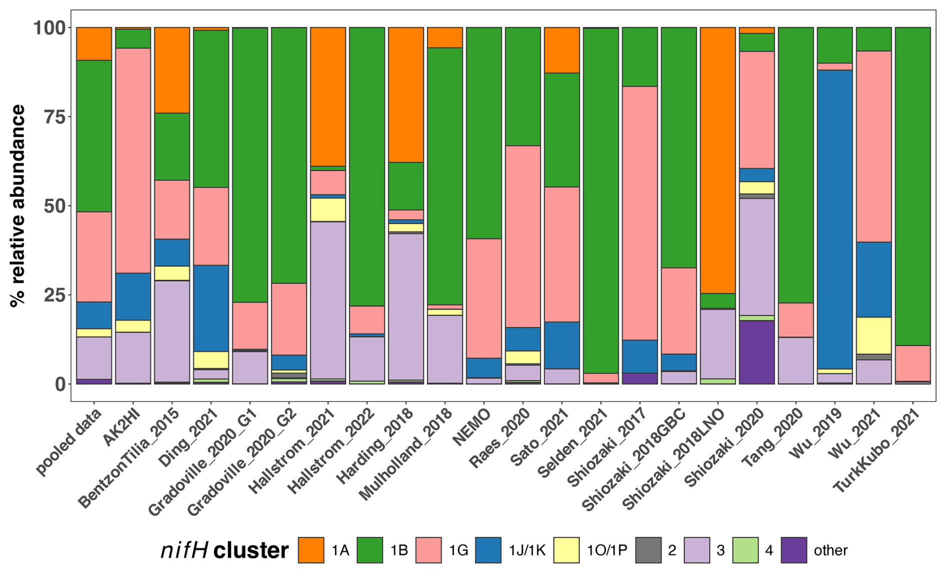
Figure 7 Study-specific diazotroph assemblage patterns in the DNA dataset. The percentages of relative abundance over the DNA dataset for each major nifH cluster are shown. The first column (“pooled data”) uses all the compiled data, while each subsequent column only uses data from the indicated study. Colors represent different nifH subclusters; “other” represents the remaining nifH clusters.

As demonstrated in a previous global analysis of diazotroph assemblages (Farnelid et al., 2011), cyanobacterial sequences (cluster 1B) dominate the samples, making up 42 % of the total relative abundance (Fig. 7). Although photosynthetic cyanobacteria would be expected to thrive in euphotic waters, NCDs are also widespread in the ocean surface (Langlois et al., 2005; Delmont et al., 2018, 2022; Pierella Karlusich et al., 2021; Turk-Kubo et al., 2022). Indeed, among the NCDs, Gammaproteobacteria (nifH cluster 1G) were the most prevalent, comprising 27 % of the total relative abundance, while Deltaproteobacteria (clusters 1A and 3) accounted for 21 % of the total relative abundance of the DNA dataset (Fig. 7). Less prominent clusters 1J/1K (Alphaproteobacteria and Betaproteobacteria) and 1O/1P (Gamma/Betaproteobacteria and Deferribacteres) were 4 % and 3 % of the relative abundance, respectively. The remaining ASVs comprised <1.5 % of the total relative abundance and came from clusters associated with nitrogenases that do not use iron (e.g., cluster 2) or that are uncharacterized (cluster 4) (Fig. 7).

Cluster 1B (cyanobacteria) were generally high in individual studies across the nifH DNA dataset, comprising ≥25 % of the community in two-thirds of the studies (Fig. 7), which is the highest of any cluster. Studies carried out in polar regions (Harding_2018, Shiozaki_2018LNO, Shiozaki_2020) and the Indian Ocean (Wu_2019 and Wu_2021) were distinct from this pattern, with low relative abundances of cluster 1B. Instead, Arctic studies had high relative abundances of clusters 1A and 3 (both primarily comprised of Deltaproteobacteria), and clusters 1J/1K (Alphaproteobacteria and Betaproteobacteria) and 1O/1P (Gamma/Betaproteobacteria and Deferribacteres) were the predominant groups in the Indian Ocean.

The second most abundant group was cluster 1G (Gammaproteobacteria), making up ca. 25 % of the total relative abundance across the DNA dataset, with study-specific relative abundances greater than 25 % in 8 out of 21 studies (Fig. 7). Members of this group were often found at high relative abundances in Pacific Ocean studies (AK2HI, NEMO, Raes_2020, Sato_2021, Shiozaki_2017), as well as in other ocean regions including the Atlantic (BentzonTilia_2015), Indian (Wu_2021) and Southern oceans (Shiozaki_2020). The notable exception is in Arctic studies (Harding_2018, Shiozaki_2018LNO), where cluster 1G was almost absent (Fig. 7).

In several studies, including BentzonTilia_2015, Hallstrom_2021, Mulholland_2018, Selden_2021, Tang_2020, and Hallstrom_2022, diazotroph assemblages had high relative abundances of putative Deltaproteobacteria (clusters 1A and 3), possibly reflecting a coastal/shelf or upwelling signature (Figs. 2 and 7). The only study with samples primarily from the Southern Ocean (Shiozaki_2020) was also the only study with a large portion of nifH cluster 1E (Bacillota).

3.3.2 Emerging global patterns in diazotroph assemblages

The nifH ASV database enables new analyses of global diazotroph biogeography in the context of environmental parameters, through co-localization with satellite and model outputs publicly available through CMAP (Ashkezari et al., 2021). To demonstrate the utility of the nifH ASV database, we present here patterns in relative abundances of nifH clusters across absolute latitude and SST in the DNA dataset. Cosmopolitan distributions were evident for gammaproteobacterial (1G) and cyanobacterial diazotrophs (1B; Fig. 8a), corroborating and extending previous findings (Farnelid et al., 2011; Shao and Luo, 2022; Halm et al., 2012; Fernandez et al., 2011; Löscher et al., 2014; Cheung et al., 2016). At low-to-middle latitudes, gammaproteobacterial (1G) diazotrophs generally had high relative abundances and were often the dominant taxa when present. However, they declined within the gyre regions, ranging between ∼25 %–50 % of the population when present, while cyanobacterial diazotrophs (1B) increased and became dominant in the subtropical gyres (Fig. 8a). Notably, cluster 1G diazotrophs reached high relative abundances in each transitional zone, before mainly disappearing at latitudes above 56° (Fig. 8a). However, as mentioned previously, sampling bias likely plays a large role at these higher latitudes where the numbers of studies and samples are sparse (Figs. 2 and 5).

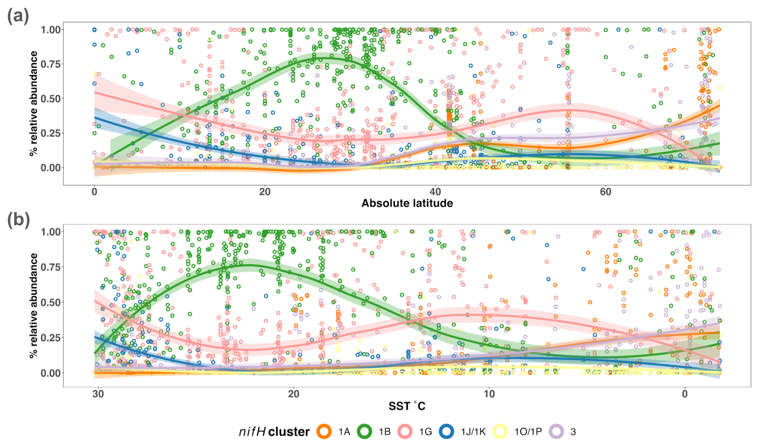
Figure 8 Influence of SST on the global distribution of major nifH clusters in the photic zone of the DNA dataset. The relative abundances of nifH genes for each major nifH cluster from every photic zone sample compiled in the DNA dataset versus (a) absolute latitude and (b) SST are shown. Smoothing averages (lines) were calculated using local polynomial regression fitting (LOESS) with 95 % confidence intervals (translucent colored areas). Each color represents a different nifH cluster. SST in (b) is from warmest to coldest temperatures to show that trends are similar to those in (a).

Clusters 1B and 1G were both detected over the full range of SST (approximately −2 to 30 °C), but peaks in their relative abundances occurred in distinct SST ranges. Cyanobacterial diazotrophs had multiple peaks in relative abundance in waters >18 °C, underscoring their dominance in tropical gyre regions (Fig. 8b). The 1G cluster also spanned the entire temperature spectrum but had notably higher presence and relative abundance above SSTs of 8 and 11 °C, respectively (Fig. 8b). The overlap between 1G and 1B has been reported previously; however, the factors controlling this are unknown (Moisander et al., 2014; Shiozaki et al., 2017, 2018a; Liu et al., 2020; Tang et al., 2020; Messer et al., 2015).

Deltaproteobacterial diazotrophs (clusters 1A and 3) were generally found in cooler, higher-latitude waters. Notably, both clusters 1A and 3 were mainly found below ∼10 °C (Fig. 8b). Deltaproteobacteria associated with cluster 1A were generally found at latitudes >32° and reached maximum relative abundances near the poles, including in the Beaufort Sea, the highest latitude region surveyed (72°; Figs. 2, 5, and 8a). The vast majority of cluster 1A Deltaproteobacteria was found at SST ≤5 °C (Fig. 8b). Although cluster 3 and 1A distributions were similar, cluster 3 showed broader spatial and temperature ranges, with consistent but low relative abundances in the subtropics and tropics (Fig. 8).

In contrast, the relative abundances of cluster 1J/1K and 1O/1P diazotrophs declined as SST decreased and latitude increased, becoming rare at higher latitudes (Fig. 8). The highest relative abundances for these clusters were observed near the Equator and, in some cases, comprised 100 % of the diazotroph assemblage in high-SST, tropical samples. These patterns suggest that temperature was an important factor controlling the narrow SST band (≥26 °C) that clusters 1J/1K and 1O/1P occupied, establishing them as the nifH clusters with the smallest geographic range in the nifH ASV database (Fig. 8).

3.4 Limits and caveats to interpreting nifH amplicon data

The PCR amplification of the nifH gene and its transcripts has been vital in advancing the knowledge of diazotroph ecology due to its high sensitivity, detecting diazotrophs at abundances that are often orders of magnitude lower than other marine microbes. This approach has facilitated the discovery of many novel diazotrophs and provided the first evidence of the widespread distribution of unicellular diazotrophs throughout the open ocean (Falcón et al., 2004, 2002; Zehr et al., 1998, 2001). Advances in HTS technologies have revealed diverse diazotrophic assemblages, including the ubiquitously distributed NCDs (Turk-Kubo et al., 2014; Shiozaki et al., 2017; Raes et al., 2020). These discoveries have fostered a new perspective of global diazotrophic ecology (Zehr and Capone, 2020), improved our models of diazotrophic distributions and global N fixation rates (Tang et al., 2019), and will continue to drive new research questions.

However, interpreting nifH PCR-based data requires the consideration of several important caveats. Diazotrophs constitute a small fraction of the total microbial community and thus often require numerous PCR cycles in conjunction with nested PCR for detection. Increasing the number of cycles can exacerbate known amplification biases (Turk et al., 2011) and increase the likelihood of detecting contaminant sequences (Zehr et al., 2003). Strategies to mitigate and assess contamination exist, e.g., by employing ultrafiltration of reagents and including blanks at different stages of the sampling and sequencing process (Bostrom et al., 2007; Farnelid et al., 2011; Blais et al., 2012; Moisander et al., 2014; Langlois et al., 2015; Fernández-Méndez et al., 2016; Cheung et al., 2021), but such strategies have not been universally adopted. Additionally, relative abundances of PCR amplicons cannot easily be related to absolute abundances. For example, the relative abundance of a taxon can change even if its absolute abundance remains constant, or the relative abundance can remain constant despite changes in the total assemblage size. Moreover, the complexity of the diazotroph assemblage can, if the HTS sequencing depth is insufficient, cause rare ASVs to go undetected or have relative abundances which are too low to interpret.

Primary objectives in studying marine diazotrophic populations include understanding the contribution of each group to N₂ fixation, the factors influencing their activity, and their global distributions. The relative abundances of nifH genes and transcripts estimated by the workflow can point to potentially significant contributors to N₂ fixation rates. Yet, the presence of nifH genes or transcripts does not always correlate with N₂ fixation rates (e.g., Gradoville et al., 2017). This underscores the need for cell-specific rates to better constrain N₂ fixation, the assemblages driving given rates, and the taxa-specific regulatory factors of N₂ fixation to better constrain global biogeochemical modeling.

Various methods are available to target specific diazotroph taxa over space and time (e.g., qPCR/ddPCR (droplet digital PCR), fluorescent in situ hybridization (FISH)-based methods). Universal PCR assays, e.g., those used in the studies compiled here (nifH1–4), are an important complement, because they better capture the overall diversity of the diazotrophic assemblage. Unlike primers designed for specific sequences, universal primers can amplify unknown or ambiguous sequences, enabling the discovery of genetic diversity. This includes microdiversity, where sequences show subtle variations from known ones, or even identifying entirely novel taxa. Primers specific to novel sequences can then be developed for use in the mentioned quantitative methods, enabling experiments to characterize the growth, activity, and controlling factors/dynamics of putative diazotrophs.

Tools like RT-qPCR, where transcript abundances are assessed directly, or FISH-based methods, where single cells are identified for cell-specific analysis, provide complementary perspectives into the activities of putative diazotrophs. Enumerating diazotrophs using techniques like these can help standardize the relative abundances associated with amplicon sequencing via matching taxa across each method. By assessing diversity and abundance simultaneously, major players can potentially be identified and monitored.

Through genome reconstruction, omics studies can enhance the characterization of putative diazotroph amplicon sequences by providing a robust suite of associated genetic data, e.g., taxonomic, phylogenetic, and metabolic. Previous studies have led to the assembly of dozens of diazotrophic genomes (Delmont et al., 2022, 2018). However, omics methods often require massive amounts of data to detect rare community members, and linking genes of interest to other genomic information, e.g., taxonomy, remains quite difficult. Gene-specific models are also required to retrieve diazotrophic information, and these models can benefit greatly from the high-quality diazotrophic sequences of the nifH ASV database. In summary, the complementary perspectives afforded by the methods just described should all be used to obtain robust insights into diazotrophic assemblages.

4 Code availability

The workflow used to generate the nifH ASV database is freely available in two GitHub repositories: one for the DADA2 nifH pipeline (https://github.com/jdmagasin/nifH_amplicons_DADA2; Morando et al., 2024a) and one for the post-pipeline stages (https://github.com/jdmagasin/nifH-ASV-workflow; Morando et al., 2024c).

5 Data availability

The nifH ASV database is freely available on Figshare (https://doi.org/10.6084/m9.figshare.23795943.v2; Morando et al., 2024b). HTS datasets for the 21 studies in the database can be obtained from the NCBI Sequence Read Archive using the NCBI BioProject accessions in Table 1.

6 Conclusions

The workflow and nifH ASV database represent a significant step toward a unified framework that facilitates cross-study comparisons of marine diazotroph diversity and biogeography. Furthermore, they could guide future research, including cruise planning, e.g., focusing more on the Southern Hemisphere and areas outside of the tropics, and molecular assay development, e.g., assays to characterize NCDs for single-cell activity rates.

To demonstrate the utility of our framework, the DNA dataset was used to identify potentially important ASVs and diazotrophic groups, establishing global biogeographic patterns from this aggregated amplicon data. Cyanobacteria were the dominant diazotrophic group, but cumulatively the NCDs made up more than half of the total data. Distinct latitudinal patterns were seen among these major diazotrophic groups, with NCDs (clusters 1G, 1J/K, 1O/1P, 1A, and 3) having a greater contribution to relative abundances near the Equator and at higher latitudes, while cyanobacteria (1B) comprised a majority of the diazotroph assemblage in the subtropics. SST appeared to restrict and differentiate the biogeography of clusters 1J/1K and 1O/1P (warm tropics/subtropics) from clusters 3 and 1A (cool, high-latitude waters) but did not play as large of a role for the biogeography of clusters 1B and 1G.

We provide the workflow and database for future investigations into the ecological factors driving global diazotrophic biogeography and responses to a changing climate. Ultimately, we hope that insights derived from the use of our framework will inform global biogeochemical models and improve predictions of future assemblages.

Appendix A

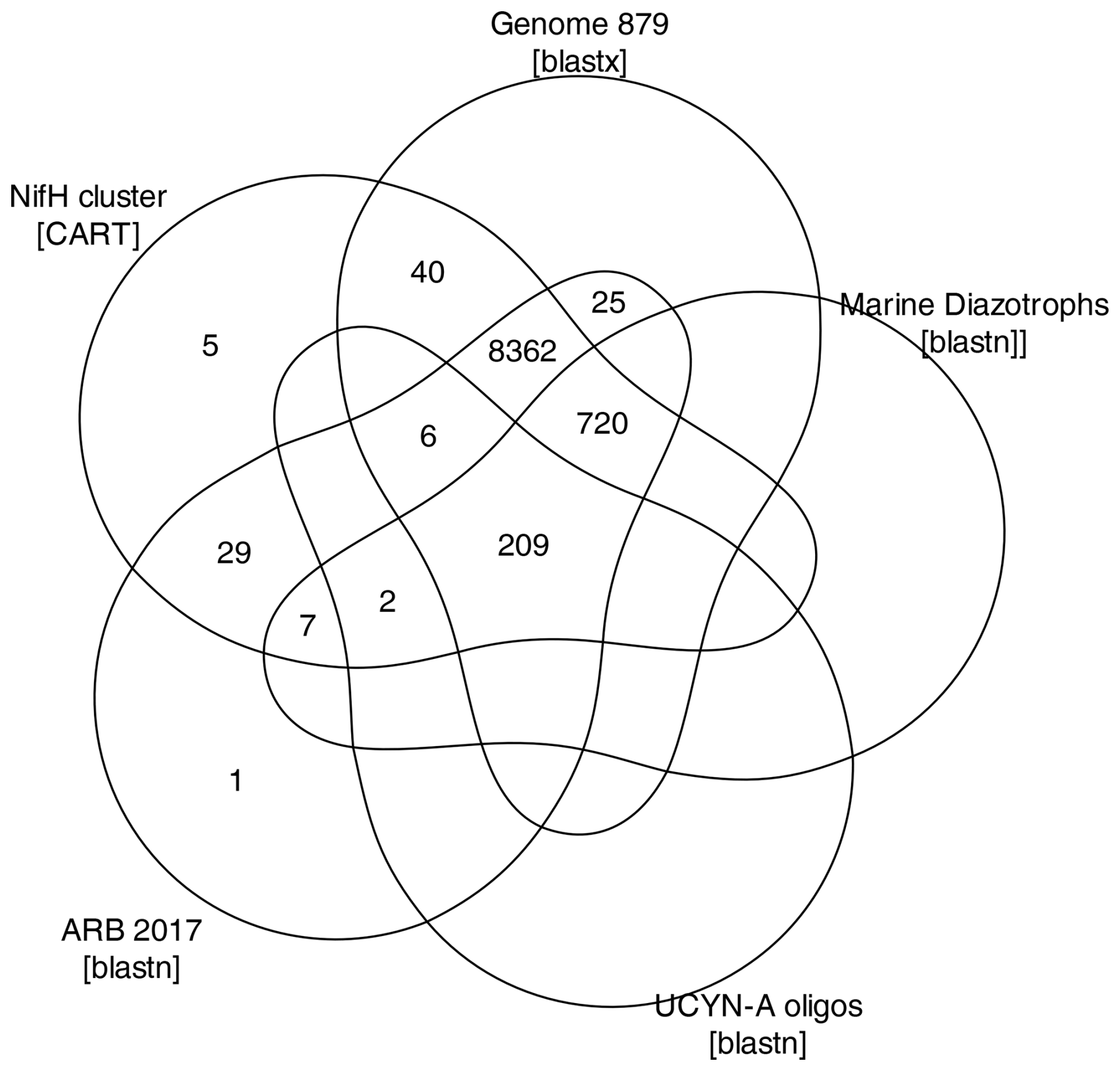
Figure A1 ASV annotations. The Venn diagram summarizes annotations assigned to 9406 ASVs during the AnnotateAuids stage of the workflow (Fig. 1). Numbers indicate how many ASVs received each type of annotation. Of the 11 915 ASVs from the preceding workflow stage (FilterAuids), only the 9406 ASVs shown received annotations.

Table A1 Compiled nifH amplicon studies. Information on all studies compiled to generate the nifH ASV database is shown, as well as studies that were not ultimately included and the reasons for this. The table provides the study ID used to refer to each dataset, the NCBI BioProject accession, the number of samples, and the DOI of the publication in which the dataset became public.

n/a: not applicable. ^a Data were obtained from authors, not the SRA. ^b For TurkKubo_2021 only surface samples (n=59) are in the first release of the nifH ASV database.

Appendix B: Read trimming method effects on workflow outputs

It is well established that error rates increase with the number of PCR cycles during Illumina sequencing (Manley et al., 2016). DADA2 trims the reads to remove the low-quality tails, an important early step that impacts the proportion of sequences retained during quality filtering and merging, as well as the ASVs detected (Fig. 1). Usually, sequencing quality plots are inspected to identify a trimming length that will, on average, cut the reads before quality declines significantly. However, inspecting tens to hundreds of quality plots (depending on the study size) is laborious and unsystematic. For the present work, the pipeline ancillary script estimateTrimLengths.R was used to efficiently identify lengths that maximized the percentages of reads retained for each study (Sect. 2.3.2). The optimized lengths appeared in the parameter files as truncLen.fwd and truncLen.rev as used by DADA2 filterAndTrim (Table 2).

An alternative to fixed-length trimming is to trim each read based on its individual quality profile, at the first position where the estimated sequencing error rate exceeds a threshold specified in the truncQ parameter to filterAndTrim (Table 2). This approach might reduce mismatches in the overlapping regions during the merge step and thus retain more read pairs. However, spurious low-quality bases could cause overly aggressive trimming, and picking a threshold that allows most sequences to overlap is not straightforward.

The quality of the raw sequencing data is a critical factor in the generation of the final ASV table. When analyzing a new dataset, testing both the fixed-length (truncLen) and quality-based (truncQ) trimming methods is suggested; they are fundamentally different, and filterAndTrim impacts all downstream DADA2 steps. If both methods produce similar ASVs and abundances, additional parameter tuning is unlikely to impact the analysis meaningfully.

To illustrate how the trimming approach can impact workflow outputs, a version of the nifH ASV database was generated as shown in Fig. 1 except that reads were trimmed at the first position where the estimated error rate was >2.5 % (truncQ = 16 in Table 2). This threshold typically produces forward and reverse ASVs of sufficient length to overlap without mismatches. The truncQ version of the database had substantially fewer samples, reads, and ASVs (Table B1), partly because truncQ appeared more affected by low-quality reads (discussed below). Only 1783 ASVs out of 9383 in the nifH ASV database were detected by both trimming methods, but they comprised 88.3 % of the total reads in the database (Table B1). The 7600 ASVs (16.7 % of reads) that were found only using truncLen had mainly low abundances and were detected mainly in one to several samples. Although truncQ was less sensitive to rare ASVs, for most studies the relative abundances of nifH groups were similar using either trimming approach (Fig. B1).

Table B1 Impact of the read trimming method on workflow outputs. The table compares the nifH ASV database, generated using fixed-length read trimming (truncLen for DADA2 filterAndTrim), to an alternative database for which reads were trimmed at the first nucleotide where the error rate was >2.5 % (truncQ = 16). No other pipeline or post-pipeline parameters were changed.

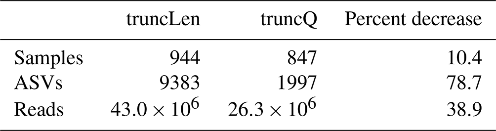
There were three exceptions where sequencing quality issues caused substantial differences in the results from truncQ and truncLen, i.e., BentzonTilia_2015, Hallstrom_2022, and Shiozaki_2020. Using either trimming method, all three studies lost high percentages of reads during filterAndTrim (Fig. 3; losses using truncQ were comparable). This indicates that sequencing errors remained after trimming (>2 errors in the trimmed forward reads and >4 in the reverse; maxEE in Table 2). However, the subsequent losses during mergePairs were much higher using truncQ (vs. truncLen), respectively, 58 % (10 %), 61 % (5 %), and 72 % (6 %) of reads. This suggests that trimming with truncQ = 16 more frequently produced reads that failed to overlap during the merge step. For these three studies, the workflow discarded many samples due to having ≤500 reads but discarded more with truncQ (vs. truncLen), respectively, n=54 (34), 59 (29), and 14 (5) samples discarded. These three exceptions suggest that truncLen-based trimming can retain substantially more reads and samples for FASTQ files with lower quality reads, which could impact relative abundances (Fig. B1).

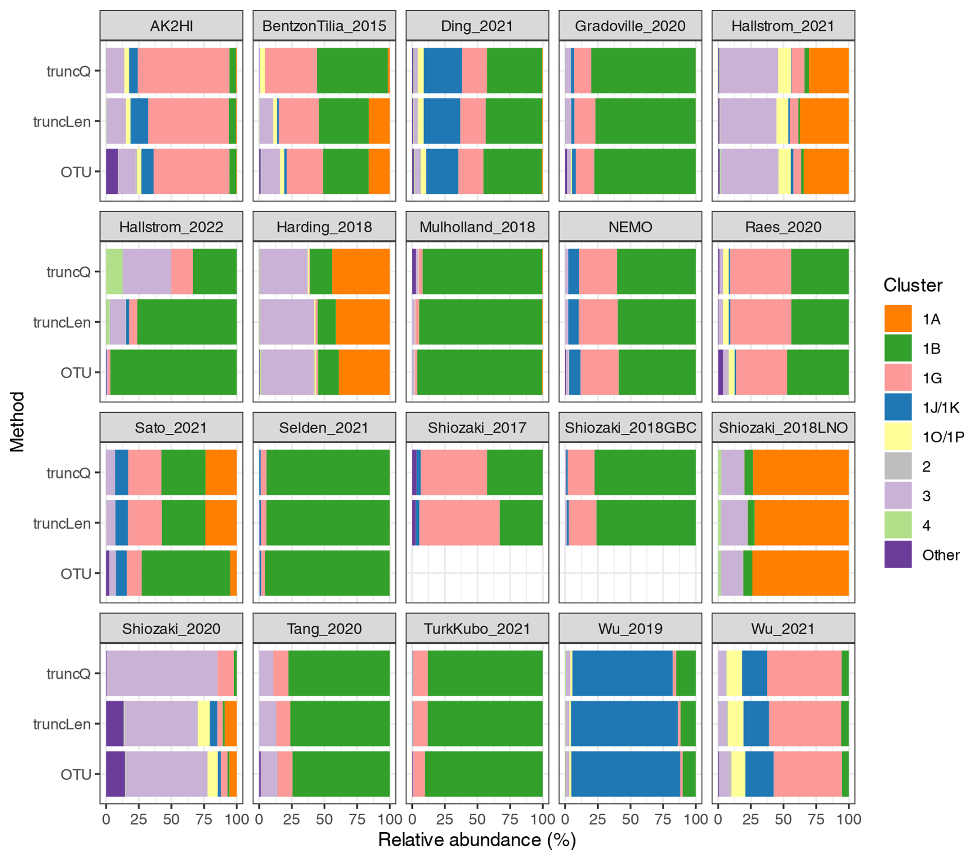
Figure B1 Relative abundances using different DADA2 trimming methods and the NifMAP OTU pipeline. The nifH cluster relative abundances are shown for each study when processed using the NifMAP OTU pipeline (Angel et al., 2018) or by the nifH workflow using two methods for trimming reads: quality-based (truncQ) or fixed-length (truncLen) methods. ASV or OTU abundances for the samples in a study were pooled to calculate the relative abundances shown. The three results for each study were calculated using only the samples that were retained by both runs of the nifH workflow. Shiozaki_2017 and Shiozaki_2018GBC used mixed-orientation sequencing libraries and could not be processed by NifMAP.

Appendix C: Comparison of communities from the workflow to previous studies

Prior to DADA2 (Callahan et al., 2016) and other approaches that distinguish fine-scale variation from sequencing errors (Eren et al., 2014, Edgar 2016b, Amir et al., 2017), most amplicon studies – for 16S rRNA as well as functional genes – processed their sequencing data into operational taxonomic units (OTUs). Usually, this meant de novo clustering the amplicon sequences at 97 % nucleotide identity and using a representative sequence from each of the OTUs (clusters) for subsequent analyses. For 16S rRNA genes, it is known that PCR artifacts and sequencing errors can inflate the number of OTUs and cause diversity to be overestimated (Quince et al., 2009; Eren et al., 2013). For nifH amplicon data, these issues have been mitigated in previously published OTU analyses by analyzing broad diazotroph groups (Table C1).

To demonstrate whether communities derived from the workflow differ substantially from those previously published, a comparison was made between the results from the nifH workflow and another nifH pipeline, NifMAP (Angel et al., 2018). NifMAP is an OTU pipeline that uses hidden Markov models in an attempt to distinguish true nifH sequences from orthologs often mistaken for nifH. NifMAP was used to generate proxies for most of the 21 studies since complete OTU sequences and abundances were not available for the 19 original studies. Using NifMAP for all studies was more systematic than trying to reproduce the original results which depended on different software and methods for quality filtering. Additionally, the workflow and NifMAP both use CART (Frank et al., 2016) to identify nifH clusters, enabling the cross-comparison of major nifH groups. Both also distinguish nifH from orthologs (the workflow using classifyNifH.sh described in Sect. 2.3.3). Only the samples that were processed by both the workflow and NifMAP were compared (n=902).

The main result was that similar diazotroph communities were detected by the nifH workflow and NifMAP (Fig. B1). For every study, they agreed on the two most abundant nifH subclusters, usually with ≤3 % difference between the relative abundances from the workflow and NifMAP. These results suggest that comparisons between new and previously published nifH amplicon studies are possible, especially if both use similarly broad taxonomic levels, e.g., nifH subclusters.

However, for two studies there were clear differences between the nifH workflow and NifMAP that speak to the utility of the workflow. For Hallstrom_2022, the workflow detected additional nifH subclusters, mainly 3 and 1G, and for Sato_20201 the workflow detected 1G and 1A at much higher levels (Fig. B1). These compositional differences likely stemmed from vastly greater numbers of reads retained by the workflow compared to NifMAP (1034 % and 264 % more reads, respectively, for the two studies; Table C1). The NifMAP logs revealed that poor read quality caused NifMAP to discard the majority of reads in the first two steps. Only 10 % of the Hallstrom_2022 reads could be merged, the lowest of any study (median 78 %, range 10 %–94 %), and 56 % of the reads from Sato_2021 could be merged. The merged reads were short for both Hallstrom_2022 (mean 174 nt) and Sato_2021 (198 nt) in comparison to all studies (median of 307 nt). NifMAP then discarded, respectively, 66 % and 58 % of the merged reads due to lengths <200 nt. In comparison, for Hallstrom_2022 the workflow discarded most reads during DADA2 filterAndTrim (using truncLen) due to sequencing errors but discarded few reads during mergePairs (Fig. 3 and Table 4). This suggests that DADA2 denoising worked very well for this dataset, because the forward and reverse ASVs were allowed at most one mismatch in their overlapping region (Table 2). In contrast, Sato_2021 had substantial losses of reads during both filterAndTrim and mergePairs (Fig. 3 and Table 4). Together, these results indicate that the nifH workflow can potentially retain more reads than NifMAP, particularly when data quality is low, with noticeable impacts on community composition.

Although community compositions from the workflow and NifMAP were mainly similar (Fig. B1), the workflow tended to retain more of the sequencing reads (Table C1). For 9 of the 18 studies analyzed by both the workflow and NifMAP, there was a <10 % difference in the number of reads retained in the final sequences (ASVs or OTUs; Table C1). However, 6 of the other 9 studies had more reads retained by the workflow (14 %–1034 %) and 3 had more reads retained by NifMAP (10 %–23 %). Although the workflow retained more reads, usually there were fewer ASVs than OTUs despite compression from clustering at 97 % nucleotide identity (Table C1). This is consistent with the known limitations of OTUs mentioned earlier, i.e., errors and overestimated diversity.

Table C1 Summary of the total reads and final sequences obtained by the workflow (ASVs) and NifMAP (OTUs) applied to the same samples. A total of 902 of 944 samples in the nifH ASV database were compared. This excludes 42 samples from Shiozaki_2017 and Shiozaki_2018GBC that used mixed-orientation sequencing libraries that could not be processed by NifMAP. The “Change (%)” column is relative to reads in OTUs. OTUs in the sixth column count clusters (97 % nucleotide identity).

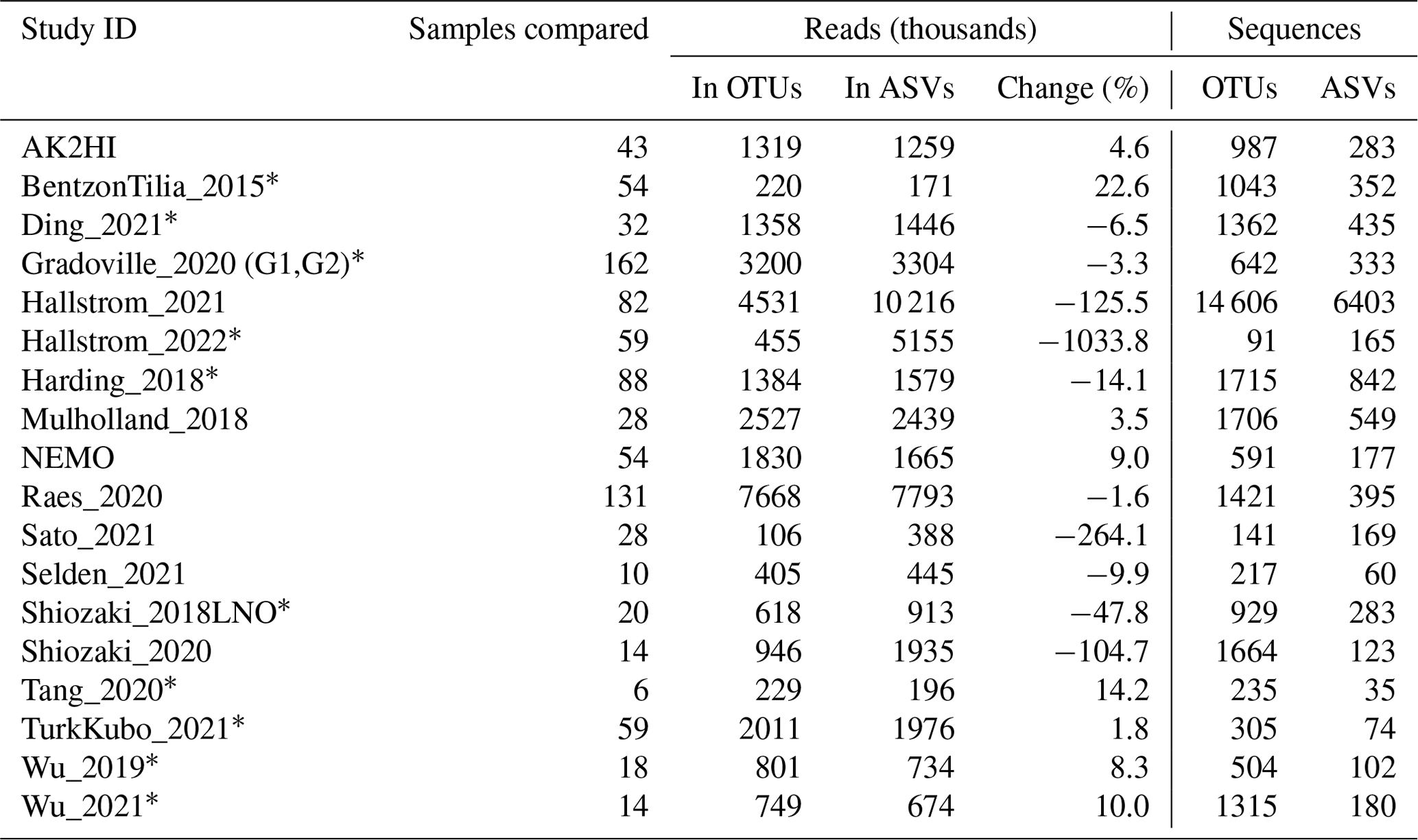
^∗ The original publication analyzed OTUs.