A derecho climatology (2004–2021) in the United States based on machine learning identification of bow echoes

Due to their persistent widespread severe winds, derechos pose significant threats to human safety and property, with impacts comparable to many tornadoes and hurricanes. Yet, automated detection of derechos remains challenging due to the absence of spatiotemporally continuous observations and the complex criteria employed to define the phenomenon. This study presents an objective derecho detection approach capable of automatically identifying derechos through both observations and model results. The approach is grounded in a physically based definition of derechos and integrates three algorithms: (1) the Python Flexible Object Tracker (PyFLEXTRKR) algorithm to track mesoscale convective systems (MCSs), (2) a semantic segmentation convolutional neural network to identify bow echoes, and (3) a comprehensive classification algorithm to detect derechos within MCS life cycles and distinguish derecho-producing from non-derecho-producing MCSs. Using this approach, we developed a novel high-resolution (4 km and hourly) observational dataset of derechos and accompanying derecho-producing MCSs over the United States east of the Rocky Mountains from 2004 to 2021. The dataset consists of two subsets based on different gust speed data sources and is analyzed to document the climatology of derechos in the United States. On average, 12–15 derechos are identified per year, aligning with previous estimations (∼6–21 events annually). The spatial distribution and seasonal variation patterns are consistent with prior studies, showing peak occurrences in the Great Plains and the Midwest during the warm season. Additionally, during the study period, derechos account for approximately 3.1 % of measured damaging gusts (≥25.93 m s⁻¹) over the eastern United States. The dataset is publicly available at https://doi.org/10.5281/zenodo.14835362 (Li et al., 2025).

1 Introduction

A derecho is qualitatively defined as a widespread, long-lived straight-line windstorm associated with a fast-moving mesoscale convective system (MCS), and the latter is named a derecho-producing MCS (DMCS). Figure 1 shows two of the most destructive derechos and their accompanying DMCSs in the United States: the June 2012 North American derecho and the August 2020 Midwest derecho. Both events lasted for over 10 h, with apparent bow echoes and extensive damaging wind gusts (≥25.93 m s⁻¹; https://www.weather.gov/mlb/wind_threat, last access: 8 April 2025). Due to the persistent widespread damaging gusts, derechos can severely damage property and threaten human lives, as exemplified by the extensive power outages and more than 10 fatalities caused by the two derechos. Ashley and Mote (2005) demonstrated that derechos could be as hazardous as and were comparable in impact to most hurricanes and tornadoes in the United States between 1986 and 2003.

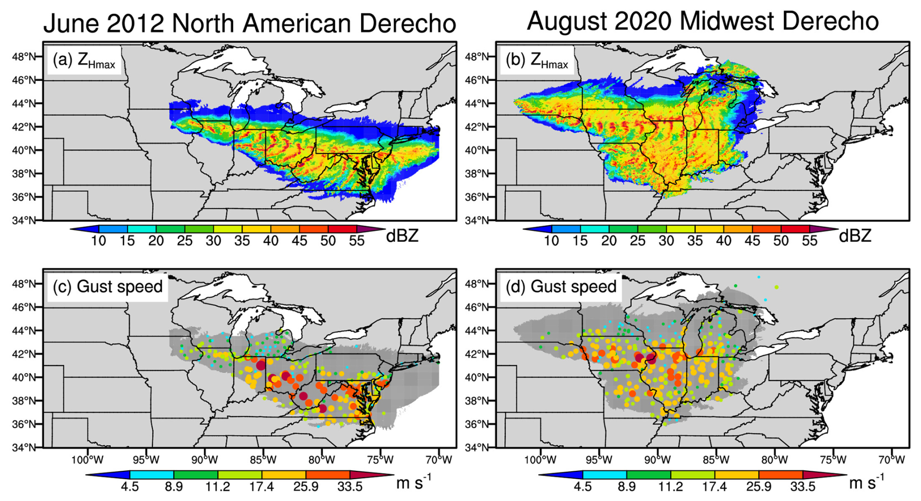
Figure 1 Spatial evolutions of the (a, b) composite (column-maximum) radar reflectivity (Z_Hmax) signatures and (c, d) surface gust speeds (colored dots) of two DMCSs. The first column is for the DMCS associated with the June 2012 North American derecho, which occurred on 29–30 June 2012, and the second column is for the DMCS that accompanied the August 2020 Midwest derecho, which occurred on 10–11 August 2020. Due to spatiotemporal overlapping, multiple Z_Hmax and gust speed values may exist for a given grid cell or weather station, in which case only the corresponding maximums are shown in the figure. In (c) and (d), the dark-gray shading refers to DMCS cold cloud coverage. The dot sizes in (c) and (d) are proportional to the gust speed magnitudes. Notably, gust speed in (c) and (d) is based on the hourly maximum gust speed (gust_{hourly_max}), which is the largest gust speed within 1 h if multiple gust speed measurements are available.

A reliable derecho dataset is foundational for understanding the underlying physical mechanisms of derecho initiation and development and their socioeconomic impacts. Johns and Hirt (1987) developed the first derecho climatology in the warm seasons of 1980–1983 in the United States by quantitatively defining a derecho as a family of downburst clusters produced by an extratropical MCS. Specifically, they required a derecho to satisfy the following six criteria.

1. There must be a concentrated area of reports with wind damage or convective gusts > 25.7 m s⁻¹, and the major axis length of the area must be at least 400 km.

2. Those wind damage or convective gust reports must show a pattern of chronological progression, as either a singular swath or a series of swaths.

3. The concentrated area must have at least three reports of either F₁ damage (32.7–50.3 m s⁻¹) (Fujita, 1971) or convective gusts of at least 33.4 m s⁻¹ separated by ≥64 km.

4. At most, 3 h can elapse between successive reports of wind damage or gusts > 25.7 m s⁻¹.

5. The associated convective system must have temporal and spatial continuity in surface pressure and wind fields.

6. If multiple swaths of wind damage or gust reports > 25.7 m s⁻¹ exist, they must be from the same MCS event.

Since then, several other studies have developed derecho climatologies during other periods using slightly different criteria (Bentley and Mote, 1998; Evans and Doswell, 2001; Bentley and Sparks, 2003; Coniglio and Stensrud, 2004; Guastini and Bosart, 2016). For example, Bentley and Mote (1998) removed the third requirement and reduced the elapsed time in the fourth condition from no more than 3 h to no more than 2 h in their derecho climatology from 1986 to 1996. In Coniglio and Stensrud (2004), the elapsed time was further changed to no more than 2.5 h, and gust reports of at least 33 m s⁻¹ were used to separate derechos of different intensities.

Although the aforementioned derecho datasets were generated using different criteria and during different periods (Johns and Hirt, 1987; Bentley and Mote, 1998; Evans and Doswell, 2001; Bentley and Sparks, 2003; Coniglio and Stensrud, 2004; Guastini and Bosart, 2016), they showed many similar derecho climatological characteristics in the United States. For example, derechos occur more frequently in the warm than cold seasons; the Great Plains, Midwest, and Ohio Valley are regions most favorable for derecho development, and few derechos occur in eastern and western coastal areas. Considering the inconsistent thresholds used in the above studies and the lack of physical mechanisms in their derecho definitions, Corfidi et al. (2016) proposed a stricter and more physically based derecho definition, which required the existence of sustained bow echoes with mesoscale vortices or rear-inflow jets and a nearly continuous wind damage swath at least 100 km wide along most of its extent and 650 km long. In addition, the wind damage must occur after the convective system was organized into a cold-pool-driven forward-propagating MCS. Most derechos satisfying this definition would be classified as “progressive” but not “serial”. A serial derecho typically originates in strongly forced environments and develops from a mature squall line with multiple embedded bow echoes. In contrast, progressive derechos generally originate from small convective clusters that grow upscale into large organized forward-propagating MCSs in synoptic environments with weak forcing (Squitieri et al., 2023; Corfidi et al., 2016).

It is difficult to develop a derecho climatology using the definition proposed by Corfidi et al. (2016) with current operational measurements, as it involves the identification of bow echoes, rear-inflow jets, and cold pools. However, rear-inflow jets and cold pools are generally associated with bow echoes (Weisman, 1993; Adams-Selin and Johnson, 2010). Once long-lived bow echoes are found in an MCS, we can expect the simultaneous existence of rear-inflow jets and cold pools. Nevertheless, identifying bow echoes, features typically identified visually from radar observations, is still challenging for large volumes of data, such as the 30+ years of data in the National Oceanic and Atmospheric Administration (NOAA) Next Generation Weather Radar (NEXRAD) archive, consisting of 159 radars. The manual examination is time-consuming and sensitive to subjective biases. The present study applies a semantic segmentation convolutional neural network (CNN) to detect bow echoes automatically from two-dimensional composite (column-maximum) reflectivity (Z_Hmax) data in the United States, which are then combined with an MCS tracking dataset and surface gust speeds to identify derechos using criteria adjusted from Corfidi et al. (2016). After manual examination and validation, we produced a high-resolution observational derecho and DMCS dataset for the United States east of the Rocky Mountains from 2004 to 2021 at 4 km spatial and hourly temporal resolution. The dataset comprises two subsets based on different gust speed data sources: one uses gust speed measurements from the global hourly Integrated Surface Database (ISD) (NOAA/NCEI, 2001), and the other exploits gust speed reports from the NOAA Storm Events Database (SED). As the first derecho climatology that utilizes a machine learning technique following physically based criteria and covers the recent decades, the dataset provides a reference for future derecho research, enabling investigation of derecho initiation and development mechanisms, climatological impacts of derechos on hazardous weather, and their potential damage to infrastructure and property.

The remainder of the paper is organized as follows. Section 2 introduces the MCS and gust speed datasets used to generate the derecho dataset. Section 3 describes the machine learning (i.e., semantic segmentation CNN) methodology to detect bow echoes, including sampling, training, and evaluation. Section 4 explains our derecho identification criteria in detail. Section 5 evaluates our derecho dataset through cross-validation of the two subsets (ISD-based vs. SED-based) and compares them with previous derecho estimations and the observational data from the NOAA Storm Prediction Center (SPC) for 2004 and 2005. Section 6 analyzes the derecho climatological characteristics. Section 7 shows how to access our derecho dataset, and the study is summarized in Sect. 8.

2 Source datasets

2.1 MCS dataset

Since previous MCS datasets only cover the period from 2004 to 2017 (Li et al., 2021; Feng et al., 2019), we use an updated version of the Python Flexible Object Tracker (PyFLEXTRKR) software (Feng et al., 2023), which exploits collocated radar signatures, satellite infrared brightness temperature, and precipitation to identify robust MCS events (Feng et al., 2019), to produce an updated 4 km and hourly MCS dataset for the United States east of the Rocky Mountains from 2004 to 2021 (Feng, 2024). Several hourly source datasets are used in the generation of the MCS dataset, including the National Centers for Environmental Prediction (NCEP)/the Climate Prediction Center (CPP) L3 4 km Global Merged IR V1 brightness temperature dataset (Janowiak et al., 2017), the three-dimensional Gridded NEXRAD Radar (GridRad) dataset (Bowman and Homeyer, 2017), the NCEP Stage IV precipitation dataset (CDIACS/EOL/NCAR/UCAR and CPC/NCEP/NWS/NOAA, 2000), and melting level heights derived from ERA5 (European Centre for Medium-Range Weather Forecasts (ECMWF) Reanalysis v5) (Hersbach et al., 2023). The MCS definition criteria are almost the same as those in Feng et al. (2019), such as the cold cloud shield (CCS) area > 60 000 km², the precipitation feature (PF, which is a continuous convective or stratiform area with surface rain rate > 2 mm h⁻¹) with a major axis length > 100 km, and the existence of 45 dBZ convective echoes, except that the duration requirement is lowered to include those convective systems lasting for just 6 h. This adjustment allows us to capture slightly shorter-lived MCSs that may produce intense wind gusts but are missed in the previous MCS datasets. Convective and stratiform radar echo classification in PyFLEXTRKR follows the Storm Labeling in 3D (SL3D) algorithm (Starzec et al., 2017), which uses horizontal texture and vertical structure of radar reflectivity from the GridRad product. Notably, the GridRad data are available for each month from 2004 to 2017 but only between April and August from 2018 to 2021. Since most derechos occur in the warm season (Ashley and Mote, 2005; Coniglio and Stensrud, 2004), missing the cold months between 2018 and 2021 does not affect our derecho climatological analyses in Sect. 6. For brevity, we do not mention the missing cold months between 2018 and 2021 in the following sections unless stated otherwise.

2.2 Surface gust speed datasets

2.2.1 ISD gust speed measurements

The ISD is developed by the NOAA National Centers for Environmental Information (NCEI) in collaboration with several other institutions. The ISD compiles global hourly and synoptic surface observations from numerous sources (e.g., the Automated Surface Observing System and the Automated Weather Observing System) into a single common format and data model. Besides internal quality control procedures conducted by the source datasets, the ISD applies additional quality control algorithms to process each observation through a series of validity checks, extreme value checks, and internal and external continuity checks (Smith et al., 2011). This study uses ISD gust speed measurements passing all quality control checks (NOAA/NCEI, 2018). Notably, there may be multiple measurements at different times within 1 h for some stations. To keep the sampling consistency across different datasets used in the derecho identification, we calculate gust_{hourly_max}, which is the largest gust speed of all available measurements within 1 h, for each observational site, unless stated otherwise. A total of 4260 observational sites provided gust speed measurements between 2004 and 2021 in the study domain, of which 3954 are over land and the rest are over the ocean or lakes (Fig. S1 in the Supplement). We have excluded one observational site (ISD station ID: 726130-14755) in the northeastern United States, which has an unrealistic number of damaging gust measurements (more than 1000 h) and is inconsistent with the surrounding sites. We note that, although we only use measurements passing all the available quality control checks, spatial quality control is missing in the ISD (Smith et al., 2011). Figure S2a shows that some sites in the eastern United States have apparently more damaging gust occurrences than their surrounding sites, but the occurrence frequencies are less than those stations around the Rocky Mountains. We do not have enough evidence to exclude them from the study. The quality of the ISD gust speed measurements will undoubtedly be a source of uncertainty for our derecho dataset. In addition, only 420 ISD sites have continuous gust measurements from 2004 to 2021, while the rest have gust measurements only during part of the study period. The availability of ISD observational sites is another source of uncertainty when identifying derechos.

2.2.2 SED gust speed reports

The SED is also maintained by the NOAA NCEI and serves as NOAA's official publication documenting storms and other significant weather phenomena that are intense enough to cause socioeconomic damage (NOAA/NCEI, 2025). The National Weather Service (NWS) compiles storm data from a wide range of sources beyond meteorological weather stations and submits them to NCEI. These sources include, but are not limited to, local and federal law enforcement agencies, government officials, Skywarn spotters, NWS damage surveys, the insurance industry, newspaper clipping services, media reports, private companies, and individuals. While the NWS strives to use the best available information, some data in the SED remain unverified due to time and resource constraints. Consequently, the dataset suffers from inaccuracies, inconsistencies, and gaps (Santos, 2016). For example, Ardon-Dryer et al. (2023) found that half of the “dust storms” recorded in the SED had visibilities larger than 1 km, indicating misclassification, while many actual dust storms with visibilities of ≤1 km were missing from the dataset. These issues were attributed in part to the diverse sources contributing to the SED and the lack of systematic verification and consistency checks. Considering these limitations, particularly the fact that many strong (≥17.43 m s⁻¹) and damaging gust reports in the SED are estimated rather than measured, the derecho and DMCS dataset developed from SED in this study is published as a supplement to the dataset derived from the ISD.

From the SED, we extract measured and estimated gusts, along with their corresponding locations and timestamps, for the period from 2004 to 2021. The raw SED files are available at https://www.ncei.noaa.gov/pub/data/swdi/stormevents/csvfiles/ (last access: 27 August 2024) (NOAA/NCEI, 2025). If a gust report is recorded as a segment containing both a start and end location with respective timestamps, we process it as two independent reports: one at the start location and time and another at the end location and time. Although the accuracy of the SED gust speeds is not guaranteed, the database provides significantly more strong and damaging gust reports than the ISD due to its inclusion of estimated gusts from various sources. Approximately 82 % of SED gust reports from 2004 to 2021 are estimated, while only 18 % are measured. However, it is important to note that not all measured strong or damaging gusts are captured in the SED. Given the distinct limitations of both the ISD and SED datasets, we apply different threshold criteria for derecho detection depending on the dataset used. These criteria are described in detail in Sect. 4.

3 Machine learning identification of bow echoes

A bow echo is a bow-shaped pattern with high-reflectivity values on a radar image, but its vague definition makes it hard to identify bow echoes extensively and efficiently using traditional methods. Instead, we train a semantic segmentation CNN to identify bow echoes automatically from two-dimensional Z_Hmax images by performing pixel-level labeling of the bow echo extent. Compared to the manual examination of radar images, machine learning can save a tremendous amount of time and eliminate subjective bias.

3.1 Bow echo samples

3.1.1 Initial manual sampling

Our initial bow echo samples are generated based on the named derechos on Wikipedia (https://en.wikipedia.org/wiki/List_of_derecho_events; last access: 19 March 2023), corresponding to 54 accompanying DMCSs in the MCS dataset. We manually labeled times with apparent bow echoes through visual inspection of hourly Z_Hmax associated with the tracked DMCSs. Each positive sample is a 384×384 px (∼1536 km × 1536 km) Z_Hmax image centered at the corresponding DMCS with a bow echo embedded (Fig. 2). The number of bow echo samples varies among different DMCSs, and 566 positive samples (with bow echoes) are obtained in total. 5400 negative samples (generally without bow echoes) are also randomly selected from the entire 18 years of radar reflectivity data embedded in the MCS dataset.

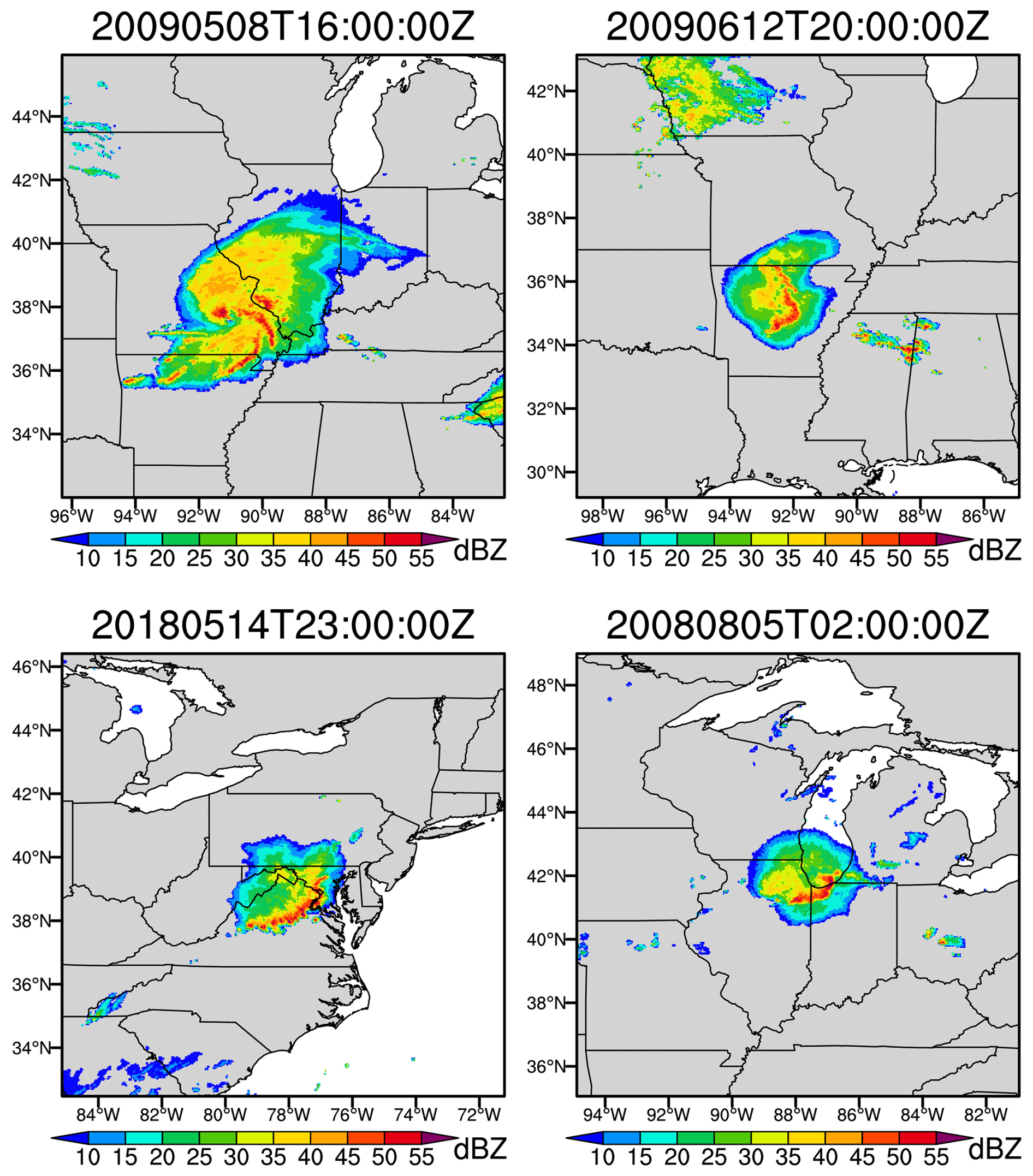
Figure 2 Four examples of bow echoes from the named derecho accompanying DMCSs. The color shading is for Z_Hmax. The subplot titles indicate the bow echo occurrence times. For example, 20130613T04:00:00Z represents 04:00 UTC on 13 June 2013.

3.1.2 CNN-based selection of additional bow echo samples

Our initial attempt at developing an automated bow echo detection scheme was to train a classifier CNN – “Dense Net” (Huang et al., 2019) – that ingests 384×384 px single-channel Z_Hmax images and outputs a single classification indicating the presence of a bow echo. Dense Nets are notable for their large number of skip connections (which create multiple paths for data to flow through the network without passing through every layer), and they can achieve comparable performance to very large classifier CNNs with only a fraction of the trainable parameters. Unfortunately, our manual inspection finds that a Dense Net trained on the aforementioned initial samples has a very high false positive rate when applied to the full radar dataset. Although this Dense Net is unsuitable for deployment, the collection of new positive samples it successfully identified allowed us to supplement the list of known bow echoes and develop a more diverse training set for the following segmentation model.

3.1.3 Pseudo-labeling

By combining the initial samples and the manually selected true positives from the low-quality Dense Net model, we built a semantic segmentation training dataset of 500 unique bow echo snapshots and corresponding hand-drawn bow echo masks. While 500 positive samples are relatively small for a deep learning application, these samples have higher diversity than the initial bow echoes generated from the named derechos on Wikipedia because they are drawn from a broader range of events, and, in general, semantic segmentation CNNs can be successfully trained with far fewer samples than image classification CNNs (Bardis et al., 2020).

A relatively low-skill version of the semantic segmentation CNN is trained using the 500 hand-labeled radar images and then applied to the entire Z_Hmax dataset. We manually review the bow echo masks produced by this segmentation model and add some of the high-quality masks to a new training dataset. We also collect some of its false positive masks as new negative samples in the new training dataset. This is a semi-supervised learning approach known as “pseudo-labeling” or “bootstrapping” (Van Engelen and Hoos, 2020; Ouali et al., 2020) and is commonly applied to semantic segmentation problems because of the high expense of hand-drawn labels (Peláez-Vegas et al., 2023). The pseudo-labels and hand labels are combined into a final training dataset with 3677 samples, including 1699 bow echoes and 1978 negative samples, which is used to train the much more skillful semantic segmentation model in Sect. 3.2.

3.1.4 Data augmentation

To combat the limited training data further, we use several data augmentation strategies when constructing training batches. During training, positive and negative samples are selected with equal probability, and a batch size of 8 is used. First, random salt and pepper noise is added to 10 % of the pixels in each sample with a probability of 0.1 (i.e., it has a probability of 0.1 to add random noise to a pixel). Second, weak random Gaussian noise with a standard deviation of 5 dBZ is added to all the pixels in each sample with a probability of 0.1. Third, samples are flipped in up–down and left–right directions, each with a likelihood of 0.5. Fourth, samples are rotated by 0, 90, 180, or 270°, each with a probability of 0.25. Fifth, samples are randomly shifted vertically and horizontally by −5 to 5 px. Sixth, the brightness of the sample image is adjusted by a random factor of −0.6 to +0.2, and the image contrast is randomly adjusted by −0.2 to 0.2. Seventh, the binary target bow echo masks are multiplied by 0.9, and random noise drawn from a uniform distribution between 0 and 0.1 is added. This is known as “soft labels”. Lastly, both positive and negative samples are blended with randomly selected negative samples by taking the pixel-wise maximum reflectivity values of the two samples with a 0.5 likelihood. This last data augmentation is unusual but works well in our application because (a) reflectivity features typically occupy only a fraction of the sample area, with most pixels being echo-free, and (b) bow echoes are high-reflectivity features. When the last data augmentation is applied to a positive sample, the resulting image will typically still contain a bow echo that matches the target mask well.

3.2 Training of U-Net 3+ CNN

Our final semantic segmentation CNN model (Fig. 3) uses the U-Net 3+ architecture (Huang et al., 2020). U-Net 3+ is a modern variant of the U-Net architecture (Ronneberger et al., 2015) and differs from the U-Net primarily in the addition of many more skip connections and its multi-resolution loss, which computes loss on rescaled classification masks generated from feature representations at various model levels.

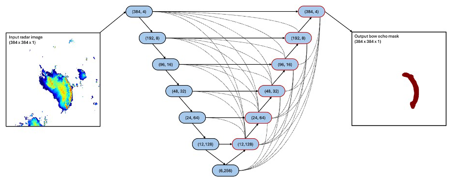
Figure 3 A diagram of our semantic segmentation CNN architecture. The CNN inputs a 384×384 px radar image (Z_Hmax scaled to 0–255) and outputs a bow echo mask of the same size. The blue rounded rectangles represent 3×3 convolutional layers, each followed by a batch normalization layer and a leaky rectified linear unit (ReLU) activation function. The first number in each blue rounded rectangle indicates the spatial size (for both the width and height) of the output tensor, and the second number represents the number of output channels. The solid arrows indicate connections in a standard U-Net architecture, with the downward arrows corresponding to 2×2 max pooling and the upward arrows corresponding to 2×2 bilinear upsampling operations. The dashed lines represent the skip connections introduced in the U-Net 3+ architecture. These skip connections use max pooling for spatial downsampling and bilinear interpolation for upsampling, followed by a 16-channel 3×3 convolutional layer with a linear activation. Layers with multiple inputs use channel-wise concatenation to combine those inputs. During training, the output tensors from the layers in the upsampling branch (blue rounded rectangles with red boundaries) are scaled to the output spatial resolution and passed through a 1-channel 1×1 convolutional layer with sigmoid activation. Training loss is computed on all 6 of the resulting masks. At the inference time, only the mask outputted from the upper-rightmost layer is used.

U-Net models were originally developed for the segmentation of biomedical imagery but have been applied to image segmentation problems in other fields and are broadly useful for any image-to-image mapping tasks where the input and target data are the same (or similar) size and shape and merging multi-resolution information from the input data is important. U-Net CNNs have been applied to a myriad of problems in the atmospheric sciences, such as segmentation (Galea et al., 2024; Kumler-Bonfanti et al., 2020), super-resolution (Geiss and Hardin, 2020; White et al., 2024), physics parameterization (Lagerquist et al., 2021), downscaling (Sha et al., 2020), and weather forecasting (Weyn et al., 2021). Perhaps most closely related to this study is Mounier et al. (2022), who used a U-Net to detect bow echoes in simulated radar reflectivity images from a forecast model. A U-Net is an appropriate choice for the segmentation of bow echoes because merging multi-resolution information is crucial for identifying these features. For example, bow echoes have high reflectivity at the pixel scale, strong reflectivity gradients in the transverse direction at the mid-scale (tens of pixels), and the characteristic bow shape at the large scale (hundreds of pixels).

Our U-Net 3+ CNN ingests 384×384 px Z_Hmax images where Z_Hmax has been clipped to a 0–50 dBZ range and then linearly mapped to a range of 0–255. It is trained using binary cross-entropy loss (Bishop, 2006) on masks generated from its 384, 192, 96, 48, 24, and 12 px resolution feature representations (Huang et al., 2020), though only the full-resolution (384×384 px) output mask is used at inference time. A detailed diagram of the model architecture is shown in Fig. 3. Notably, although the model is trained using 384×384 px samples, it is a fully convolutional model and can process inputs of variable sizes.

We use the Adam optimizer (Kingma and Ba, 2014) with the Keras default settings (Ketkar, 2017) and an initial learning rate of 0.001 for training. The U-Net 3+ CNN is first trained for 60 epochs composed of 1000 randomly generated training batches of 8 samples each. Then, we decrease the learning rate to 0.0001 and train the CNN for an additional 20 epochs. The training duration is determined by performing an initial 5 rounds of training with 5-fold cross-validation and approximating the epoch numbers to reduce the learning rate and stop training when the mean intersection over union metric plateaus for the validation set. Instead of random shuffling, the validation sets are separated from the training dataset in temporally contiguous chunks to avoid any overlap because, sometimes, multiple samples may be drawn from different times of the same convective system.

3.3 Evaluation of the semantic segmentation CNN

We apply the trained U-Net 3+ CNN to the entire Z_Hmax dataset and obtain potential bow echo masks over the United States between 2004 and 2021 (Fig. 4). As a final post-processing step, we ignore “bow echo” masks with less than 20 px (∼320 km²), which are too small to be classified as bow echoes.

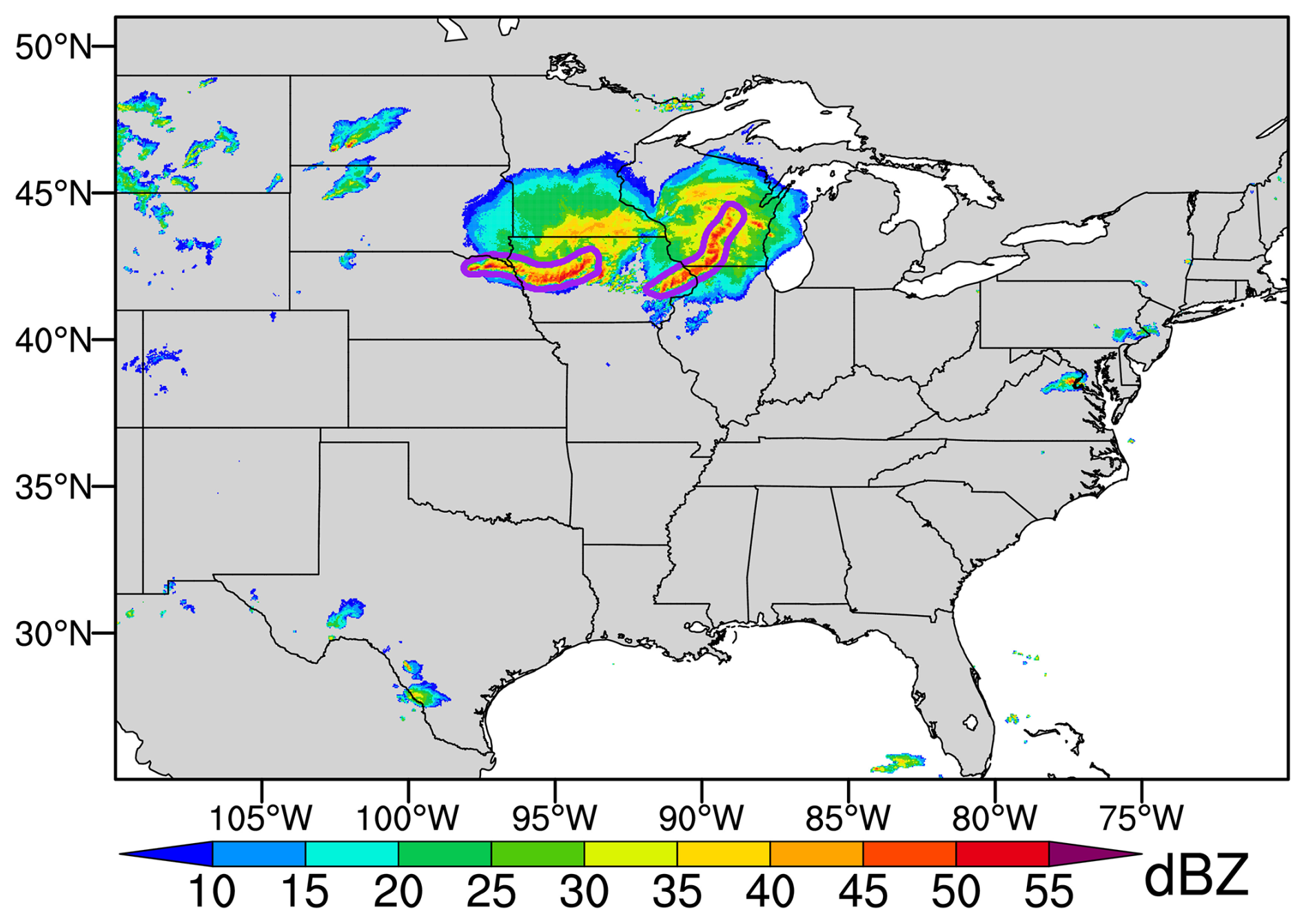
Figure 4 Examples of the U-Net 3+ CNN-identified bow echoes (purple contours) based on Z_Hmax (color shading) at 05:00 UTC on 17 June 2014.

Instead of validating our segmentation model at a pixel scale, as we had done during the training stage, we prefer evaluating its performance in detecting bulk bow echo features. In other words, we care about whether the segmentation model can recognize the existence of bow echoes and capture their rough locations. Minor spatial biases in bow echo coverage do not much affect our derecho identification described below, which contains various flexible criteria to minimize their impacts, such as the buffer zone within 100 km of bow echoes. We also choose to validate the segmentation CNN specifically using MCS events where high-reflectivity features are present. Identifying low-reflectivity and echo-free images as non-bow echoes is desirable for our segmentation model but trivial and not of particular interest for creating a derecho climatology.

To build a testing dataset, we randomly select 217 MCS-associated Z_Hmax images in 2010 based on the following requirements. Each image is from a different MCS event. The images have variable sizes and contain the full spatial extents of the MCSs at the selected times; however, they must be at least 192×192 px and cannot be drawn from a day that also has a sample in the training dataset. Three of the authors independently assessed the presence of bow echoes in each image, the results of which are then compared to the segmentation CNN (Table 1). Overall, the CNN model identifies 57 bow echoes, while human labelers 1, 2, and 3 identify 46, 76, and 66, respectively. The average human–human agreement and F₁ scores are 82 % and 0.69, while the average human–CNN agreement and F₁ scores are 82 % and 0.67 (Table 1). The test indicates that, on the one hand, the detection of bow echoes in radar images is prone to subjective bias; on the other hand, the performance of the segmentation CNN is comparable to that of a human in identifying bow echoes. We emphasize that the CNN bow echo identification is only one component in our following derecho detection criteria, and the adverse impact of this uncertainty is mitigated by other constraints (e.g., almost continuous bow echo existence and strong gusts in proximity with bow echoes).

Table 1 Evaluation of the performance of the segmentation CNN in the bow echo identification.^a

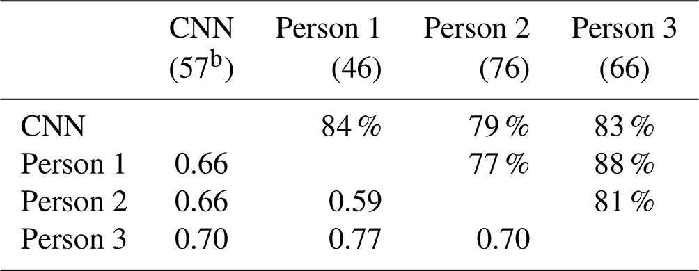
^a The upper triangular part of the table (percentages) shows agreement between two independent identifications $\left(\mathrm{agreement}=\frac{\mathrm{TP}+\mathrm{TN}}{\mathrm{TP}+\mathrm{TN}+\mathrm{FP}+\mathrm{FN}}\right)$, and the lower triangular part shows F₁ scores $\left(F_{\mathrm{1}}=\frac{\mathrm{2}\mathrm{TP}}{\mathrm{2}\mathrm{TP}+\mathrm{FP}+\mathrm{FN}}\right)$, which is a better indication of the ability to agree on positives when positives are a minority (Taha and Hanbury, 2015). Here, TP denotes true positive, TN refers to true negative, FP is false positive, and FN is false negative. Notably, for the comparison between any two independent identifications, we consider one “true” and evaluate the other against it (which set of classifications is considered true does not impact these two metrics). ^b The number of identified bow echoes from the 217 images.

We match the segmentation-CNN-detected bow echoes with MCS events from the MCS dataset and identify those MCS-associated bow echoes, which are used to identify derechos in the following section. Figure 5 shows the spatial distribution of MCS-associated bow echo occurrences from 2004 to 2021, which is similar to the MCS spatial distribution with more frequent occurrences in the Great Plains (Li et al., 2021).

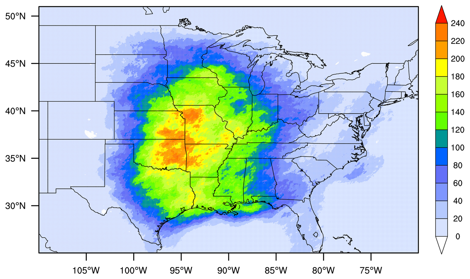
Figure 5 Spatial distribution of the number of MCS-associated bow echoes from 2004 to 2021. Here, we used bow echo masks produced by the segmentation CNN and excluded bow echoes that did not overlap with MCS events. This figure excludes bow echoes from those non-derecho-producing MCSs that overlap with tropical cyclones (TCs) from the International Best Track Archive for Climate Stewardship (IBTrACS) Version 4 data over the North Atlantic basin (Knapp et al., 2010) following the approach of Feng et al. (2021).

4 Derecho identification

4.1 Derecho definition

As mentioned above, we adopted the derecho definition proposed by Corfidi et al. (2016) but revised certain criteria based on previous studies (Johns and Hirt, 1987; Bentley and Mote, 1998) and dataset limitations to facilitate objective identification of derechos. Our final criteria are summarized below, with detailed explanations provided afterward (Fig. 6).

1. A derecho must be attached to an MCS from the MCS dataset.

2. The derecho must persist for at least 5 h, with a bow echo present for at least 80 % of its lifetime. In addition, gaps between successive bow echo occurrences cannot exceed 2 h. All bow echoes must belong to the same bow echo series, as defined in the subsequent explanation.

3. The derecho bow echo series must exhibit forward propagation based on two modified criteria from Corfidi et al. (2016):

   • The acute angle between the averaged bow echo orientation and the bow echo series' propagation direction must exceed 45° (Fig. 6).

   • The propagation speed of the bow echo series must be at least 30 % greater than the background mean wind speed at 500 hPa, derived from ERA5 data. The methodology for calculating the averaged bow echo orientation, the bow echo series' propagation direction and speed, and the background mean wind speed is detailed in Appendix A.

4. Derecho-associated gust speed criteria vary based on the gust speed source dataset.

   • For ISD data, within 100 km of the derecho-accompanied bow echoes (termed the “derecho area”), there must be at least 10 sites with strong gusts (≥17.43 m s⁻¹) and at least 1 site with damaging gusts (≥25.93 m s⁻¹).

   • For SED data, at least 10 locations must report damaging gusts.

   • The fraction of sites with strong/damaging gusts (ISD) or damaging gusts (SED) must be ≥20 %.

   • Gaps between successive strong (ISD) or damaging (SED) gust reports cannot exceed 2 h.

   • The gust swath must be at least 650 km in length and 100 km in width. Swath length and width calculations are explained below.

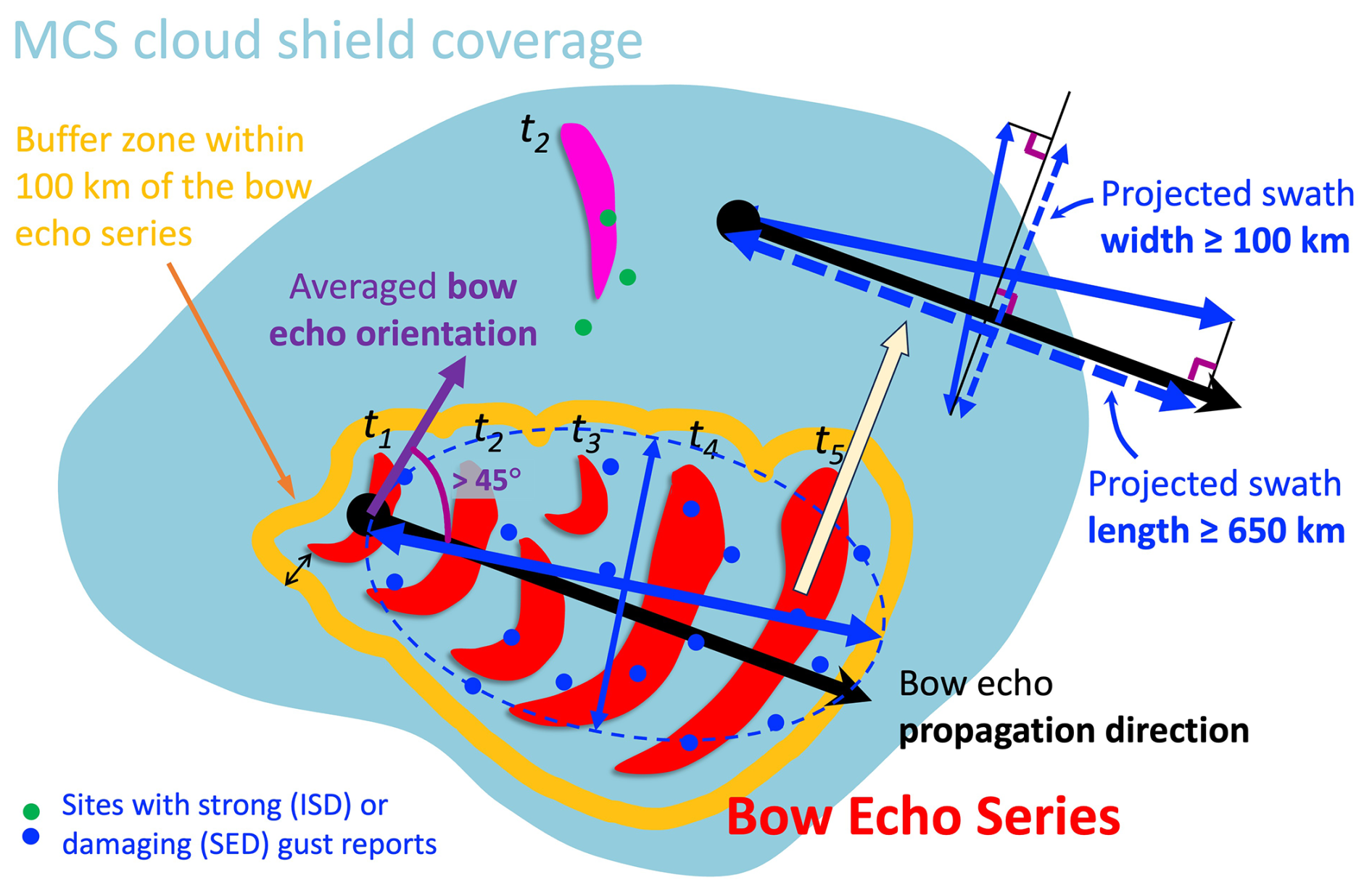
Figure 6 Schematic of the automated detection algorithm. Red and pink objects represent bow echoes. At time t₂, there are two bow echoes belonging to different bow echo series due to their great distance from each other. In contrast, the two bow echoes at t₃ are from the same bow echo series since they are close to each other. The pink bow echo at t₂ is far from the bow echoes at t₁ and t₃. Therefore, they belong to different bow echo series. The sites (green dots) with strong (for ISD) or damaging (for SED) gusts outside the 100 km buffer zone of the bow echo series (i.e., the derecho area) are excluded from the strong (ISD) or damaging (SED) gust swath calculation. The black arrow indicates the propagation direction of the bow echo series, and the violet arrow indicates the averaged bow echo orientation. Their acute angle must be > 45° for a derecho. The upper-right corner illustrates how the major and minor axis lengths of the gust-fitted ellipse are projected onto another coordinate that is parallel to the bow echo series' propagation direction to calculate gust swath length and width.

4.2 Explanation of key criteria and adjustments

4.2.1 Criterion 1: MCS association

This is a straightforward requirement and a major advantage of our approach. Due to the lack of a reliable MCS dataset, previous studies often spent considerable effort identifying spatiotemporally continuously propagating convective systems (Squitieri et al., 2023).

4.2.2 Criterion 2: bow echo occurrence and series definition

The 80 % bow echo occurrence threshold and the ≤2 h lapse time between consecutive bow echoes account for uncertainties in the segmentation CNN identification process and the diversity of MCS events.

A bow echo series was defined in two steps.

1. Spatial grouping. Within a given MCS, bow echoes occurring in the same hour are categorized into separate series if they are more than 100 km apart.

2. Temporal linking. Successive bow echoes (no more than 2 h can elapse between their occurrences) are considered part of the same series if they are less than 200 km apart, even if they were initially classified as separate series.

Due to merging or splitting or the complex nature of some convective systems, a bow echo at 1 h may be far from the bow echoes right after or before that hour or another bow echo during that hour (Fig. 6). In such a rare situation, these bow echoes are unlikely to be caused by the same physical process and, therefore, do not belong to the same bow echo series (Fig. 6). The above stepwise approach ensures that bow echoes from different physical processes are not incorrectly grouped.

4.2.3 Criterion 3: forward-propagation adjustment

We modify the Corfidi et al. (2016) criterion of “nearly orthogonal” to >45° for the acute angle between the averaged bow echo orientation and the bow echo series' propagation direction. This adjustment

• accounts for segmentation CNN uncertainties, particularly in the propagation direction estimation, and

• reduces false exclusions caused by minor variations in orientation.

4.2.4 Criterion 4: gust speed and swath calculation

The 20 % fraction threshold was introduced to exclude MCSs potentially associated with extratropical cyclones, which often produce isolated strong or damaging gusts but weaker gusts across most sites. It is noteworthy that this criterion is primary applicable to ISD data, and its implementation for SED data excludes only one MCS from being considered a potential DMCS.

To determine the gust swath length and width, we did the following:

1. We fit an ellipse around sites with strong (ISD) or damaging (SED) gusts in the derecho area (Fig. 6).

2. Since the ellipse may not align with the bow echo series' propagation direction, we project its major and minor axes onto a new coordinate system based on the bow echo propagation direction, as shown in the upper-right corner of Fig. 6. The projected major or minor axis length that is parallel to the bow echo propagation direction is the gust swath length, and the projected minor or major axis length that is perpendicular to the propagation direction is the swath width. Notably, both major and minor axis lengths can be projected parallelly and perpendicularly. If a major axis length is projected parallelly, the minor axis length must be projected perpendicularly, and vice versa. Thus, we obtain two pairs of swath length and width measurements.

3. We consider the uncertainties in the bow echo propagation direction when conducting the projection. In detail, we conduct projections iteratively by varying the propagation direction values with an interval of 0.2° within ±10° of the initial calculated bow echo series' propagation direction. Therefore, we obtain $\left(\frac{\mathrm{20}}{\mathrm{0.2}}+\mathrm{1}\right)\times \mathrm{2}=\mathrm{202}$ pairs of swath length and width in total. As long as one pair of swath length and width has a length ≥ 650 km and a width ≥ 100 km, Criterion 4 is satisfied.

If no derecho is identified for a given MCS using the above definition criteria, we can relax the distance requirement (100 km) in Criterion 4 to be within 200 km of the derecho-associated bow echoes that satisfy the condition that there is no bow echo from the same bow echo series 1 h ago or later during the derecho's lifetime. If the bow echo is in the first hour of the derecho's lifetime and there are no bow echoes for the corresponding MCS 1 h ago, we can also extend the distance threshold to 200 km. This is similar to the bow echo in the last hour of the derecho's life cycle but without CNN-identified bow echoes 1 h later. Notably, the distance extension is optional. For the bow echoes satisfying the above conditions, the distance threshold can be either 100 or 200 km. Using 100 km is superior to using 200 km until we find a derecho if it exists. The distance extension is also intended to minimize the impacts of the bow echo identification error. If a bow echo is missed in the semantic segmentation procedure, extending the distance threshold can include strong and damaging gusts associated with the missed bow echo, thus slightly reducing the derecho detection error.

We emphasize that, in Criterion 4, our ISD gust speed criteria are weaker than the SED gust speed criteria as well as those of previous studies (Squitieri et al., 2023; Bentley and Mote, 1998; Johns and Hirt, 1987), which also estimated the gust swath based on SED damaging gusts. As mentioned in Sect. 2.2.2, most SED gust reports are estimates, while ISD provides gust measurements from weather stations. SED estimates can capture potential damaging gust occurrences over a much larger area, although with large uncertainties. In contrast, due to the limited coverage of observational sites, real-time ISD measurements may miss substantial damaging gust occurrences in nearby regions. Therefore, we lower the gust speed criteria to capture potential derechos when using ISD measurements. This does not mean that the ISD-based derechos are weaker than the SED-based ones or even not derechos, as elaborated in Sect. 5.

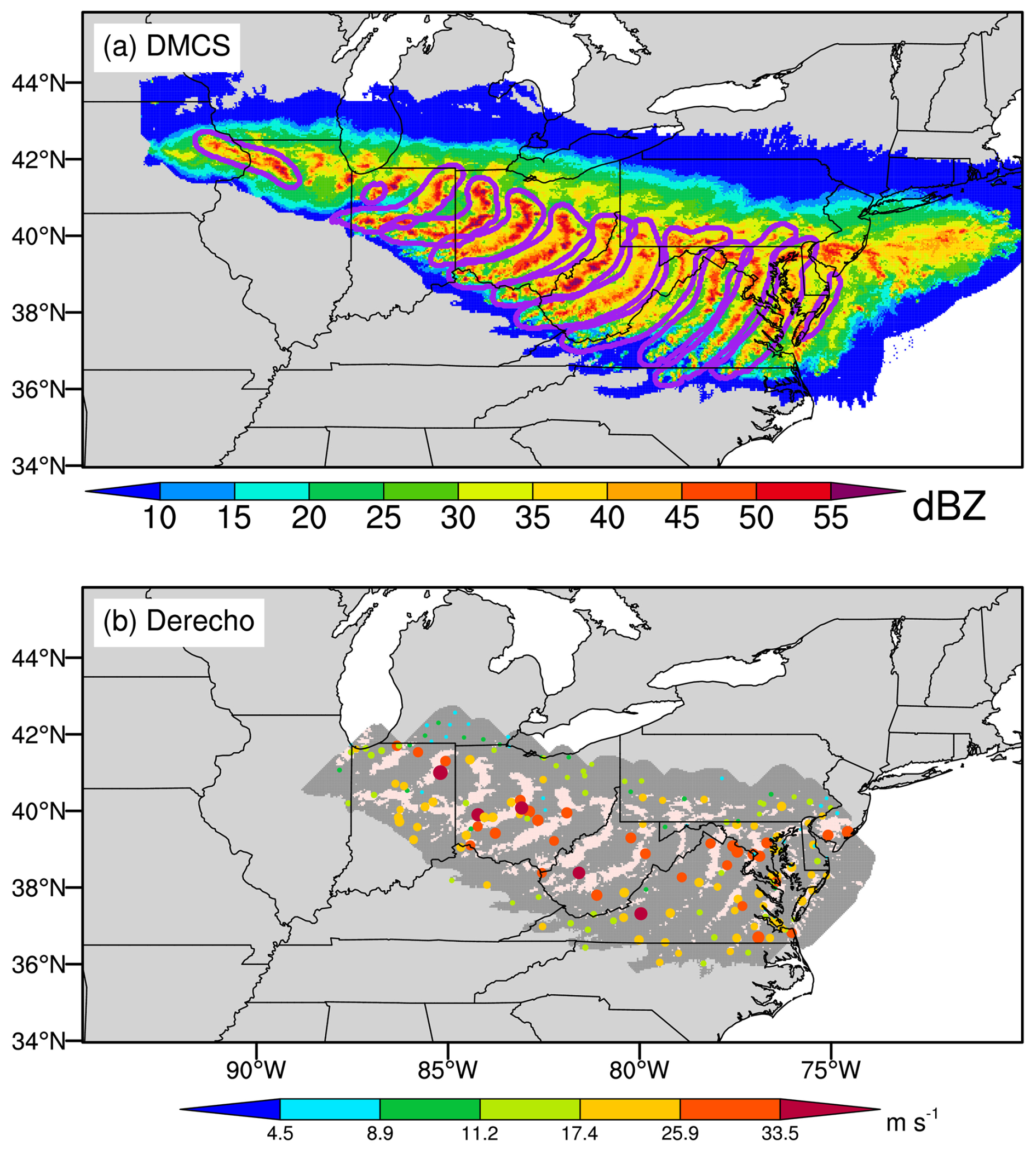
Figure 7 (a) Spatial evolution of Z_Hmax (color shading) and CNN-identified bow echoes (purple contours) from the DMCS associated with the June 2012 North American derecho. (b) Similar to (a) but for the derecho period. The derecho lasted from 17:00 UTC on 29 June to 06:00 UTC on 30 June 2012. The misty-rose shading in (b) corresponds to Z_Hmax≥40 dBZ, while the gray shading refers to the derecho area. Colored dots are the same as those in Fig. 1c, except only the derecho-associated gust measurements are shown.

4.3 Derecho detection results and post-processing

Using ISD gust measurements, the objective detection algorithm identified 245 derechos and associated DMCSs between 2004 and 2021. A notable example is the June 2012 North American derecho (Fig. 7). Figure 7a displays the CNN-identified bow echoes of the DMCS, and Fig. 7b shows the derecho area and associated gust speeds. As expected, the derecho produced widespread strong gusts.

To further refine the ISD dataset, we manually reviewed all detected derechos and DMCSs, removing 31 false detections due to erroneous bow echo identification (Fig. S3). In addition, we examined 1099 MCS events that produced extensive strong (≥10 observational sites) and damaging (≥1) gusts over land areas with a strong and damaging gust swath (fitted ellipse) of at least 650×100 km² (the ellipse's major and minor axis lengths). Our manual examination primarily focuses on bow echo identification errors but also slightly lowers the forward-propagating criteria thresholds for two potential derechos. For those MCSs that are potential DMCSs based on our visual inspection, we manually labeled their bow echo occurrences that failed the segmentation identification during potential derecho lifetimes (Fig. S4) and reran the automated derecho detection algorithm. Finally, 60 additional derechos were added, bringing the final total to 274 ($\mathrm{245}-\mathrm{31}+\mathrm{60}=\mathrm{274}$).

Using the same procedures for SED gust reports, we identified 220 derechos.

5 Dataset evaluation and uncertainty

5.1 Evaluation against existing datasets

Between 2004 and 2021, our automated detection algorithm identified 274 derechos (∼15 per year) using ISD gust measurements and 220 derechos (∼12 per year) using SED gust reports. These numbers fall within the range of previous estimations (6.1–20.9 per year) based on a 400 km swath length threshold and conventional derecho definitions, as introduced in Sect. 1 (Squitieri et al., 2023; Johns and Hirt, 1987; Bentley and Mote, 1998; Evans and Doswell, 2001; Guastini and Bosart, 2016; Ashley and Mote, 2005). However, our derecho counts are substantially higher than those reported by Corfidi et al. (2016), who identified only 25 SED-based derechos in the warm seasons of 2010–2014 using a 650 km swath length threshold. Our derecho numbers are also higher than those from Squitieri et al. (2025b), who identified 70 SED-based derechos during 2000–2022 based on the physically based definition criteria from Corfidi et al. (2016) but with much stricter gust requirements (e.g., at least five reports of very damaging gusts (≥33.53 m s⁻¹)) for a 400 km long gust swath (Squitieri et al., 2025a, b). The discrepancies among the present study, Corfidi et al. (2016), and Squitieri et al. (2025b) could be attributed to the different gust criteria used in the derecho definitions but also likely stem from differences in the methods used to calculate gust swath length and width, the criteria for forward propagation, and the diverse observational source datasets used in the derecho detection.

To further evaluate our dataset, we compare it against the NOAA Storm Prediction Center (SPC) derecho data from 2004 and 2005 (https://www.spc.noaa.gov/misc/AbtDerechos/annualevents.htm, last access: 17 November 2023) (Table 2). This dataset provides detailed timings and locations of derechos or convective windstorms of near-derecho size, and it is the only available dataset that we can use to evaluate our derecho dataset at the event scale. However, it is important to note that the NOAA SPC data do not explicitly distinguish between derechos and convective windstorms of near-derecho size, and they rely on the conventional derecho definition, which can significantly influence derecho counts. Additionally, the NOAA SPC data are based on SED gust reports and lack an underlying MCS database.

Table 2 Evaluation of our derecho dataset against the NOAA SPC data in 2004 and 2005.

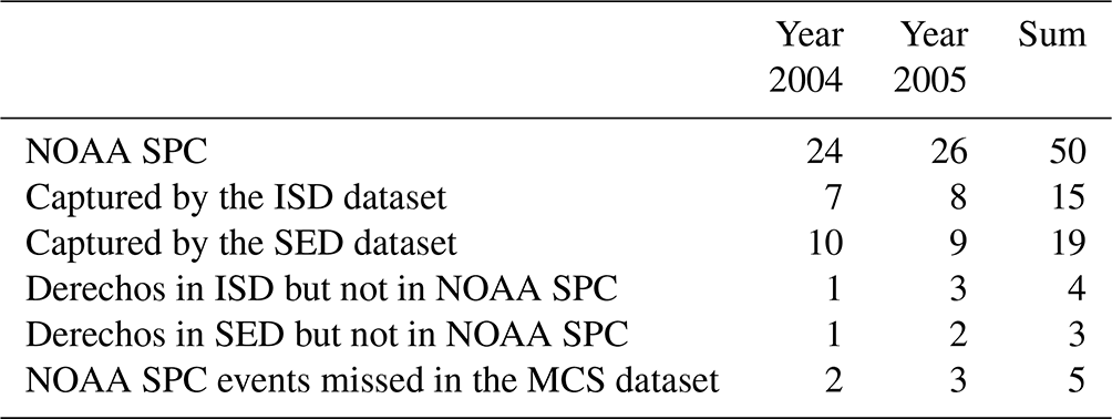
The NOAA SPC dataset contains 50 derechos and near-derecho size convective windstorms for 2004 and 2005, 15 of which are detected by our algorithm using ISD gust measurements. The number increases to 19 when using SED gust reports. Five of the 50 events are entirely absent in our MCS dataset, possibly because their associated MCSs moved too rapidly to satisfy PyFLEXTRKR's 50 % areal overlap criterion using hourly satellite and NEXRAD datasets or because they failed to meet other MCS requirements in PyFLEXTRKR (Feng et al., 2019). The remaining discrepancies arose from factors such as an insufficient number of damaging gust reports or bow echoes, too small a gust swath, or a lack of forward propagation. Conversely, our detection algorithm identified several derechos (4 from ISD and 3 from SED) that are not present in the NOAA SPC dataset. Overall, while most derechos identified by our algorithm were captured in the NOAA SPC data, our derecho counts were notably lower due to our stricter physically based derecho definition, which reduced the number of events classified as derechos compared to conventional definitions.

Cross-validation between the ISD-based and SED-based datasets further supports the robustness of our detection algorithm (Fig. 8). A total of 172 derechos were detected by both datasets, while 48 events were identified only in SED and 102 events are unique to ISD. Figure 8 also highlights discrepancies between the two datasets, with more ISD-based than SED-based derechos in 2008, 2010, 2014, 2015, 2019, and 2020, while their counts remain similar in other years. Despite these differences, the two datasets exhibit similar interannual variability, with a temporal correlation coefficient of 0.72. The general agreement between the two datasets supported our decision to use different gust speed thresholds for ISD and SED in the detection algorithm. However, the observed discrepancies also underscored the critical role of the source datasets in influencing detection results, highlighting the need for more reliable gust speed observations.

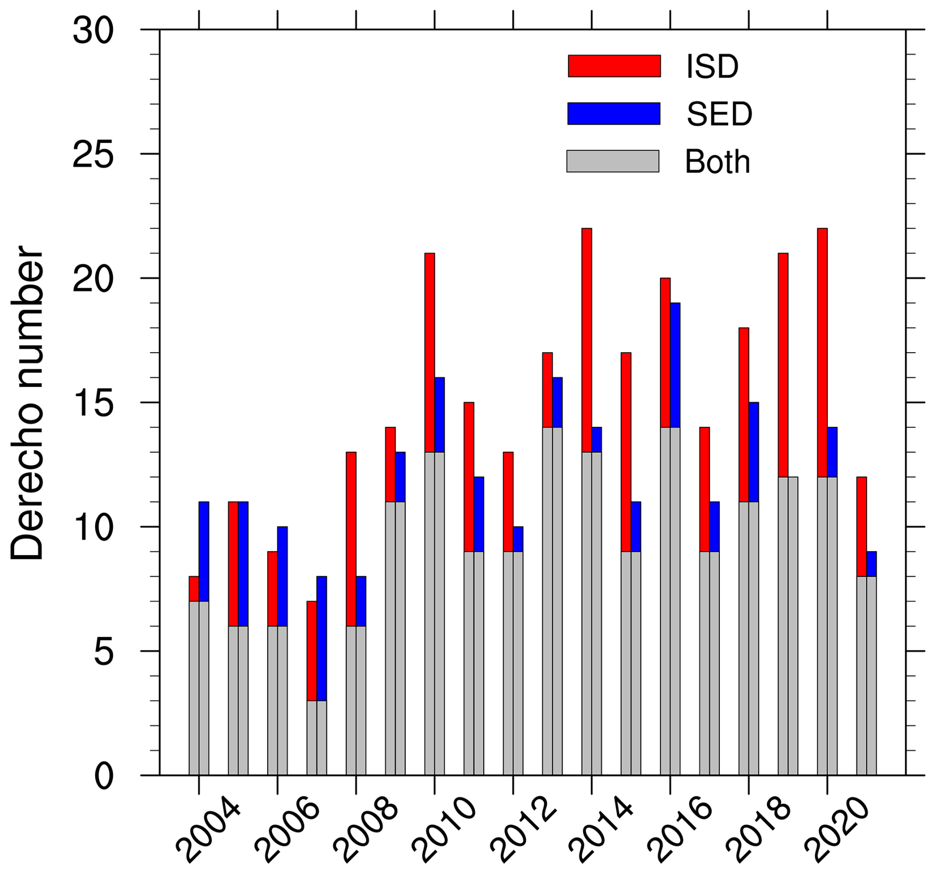
Figure 8 Bar chart of the annual derecho numbers from the ISD-based and SED-based datasets from 2004 to 2021. Gray shading denotes derechos captured by both datasets, red shading refers to derechos only identified when using ISD gust observations, and blue shading represents SED-only derechos.

5.2 Discussion on dataset uncertainty

Besides the uncertainties in gust speed observations, we acknowledge additional sources of uncertainty affecting our dataset.

5.2.1 Uncertainty from the MCS dataset

As noted in our evaluation against the NOAA SPC data, uncertainties arose from the MCS dataset used in derecho detection. The 50 % areal overlap threshold in PyFLEXTRKR, which links consecutive cold cloud shields (CCSs), may fail to capture very fast-moving convective systems using hourly satellite observations and NEXRAD data. Lowering this threshold would undoubtedly increase the number of identified MCSs and derechos, but it could also introduce false tracks that do not belong to the same storm system. The 50 % threshold is widely used in various versions of the FLEXTRKR algorithms (Li et al., 2021; Feng et al., 2023; Feng et al., 2019) and other tracking algorithms based on overlap (e.g., Whitehall et al., 2015). While we maintained this threshold in our study, users should be aware of uncertainties related to adjustable parameters (e.g., areal overlap threshold, MCS duration, and major axis length) and limitations in the observational datasets used by PyFLEXTRKR (Feng et al., 2019; Li et al., 2021).

5.2.2 Uncertainty from the bow echo identification

Another key uncertainty arose from the segmentation CNN used to identify bow echoes. While our evaluation in Sect. 3.3 confirms high accuracy, we acknowledge that some derechos may be missed, while some non-derechos may be falsely classified as derechos due to the bow echo identification errors. To mitigate this issue, we conducted extensive manual verification of derecho and DMCS events, as well as of other MCS events producing widespread strong gusts. However, the manual examination introduces subjective biases, and completely eliminating bow echo identification uncertainties remains challenging.

5.2.3 Uncertainty from derecho definition criteria

Our detection algorithm relied on several adjustable parameters and methodological choices, all of which influenced the number of identified derechos. For example, to reduce the ISD-based derecho count to the SED-based level, we had to increase the ISD gust speed threshold in Criterion 4 in Sect. 4.1 from 17.43 to 18.5 m s⁻¹; using the latter threshold produced a derecho number of 229, 152 of which overlapped with the SED-based derecho dataset. However, when we required at least five very damaging gust reports when using SED, the derecho count decreased substantially from 220 to 125, which is still larger than but much closer to the estimates by Squitieri et al. (2025b) (70 derechos between 2000 and 2022). As the first climatological derecho dataset to incorporate bow echoes and provide detailed event tracking, a full uncertainty assessment of all tunable parameters is beyond the scope of this study. However, our sensitivity tests indicated that changes to key parameters (e.g., reducing the strong gust fraction threshold to 10 % or the number of sites with strong gust reports to 5) do not substantially alter the derecho spatial distribution or seasonal variation patterns (see Sect. 6). Furthermore, our dataset was designed to be flexible: we store all key parameters (e.g., gust swath length and width and bow echo series' propagation speed), allowing users to apply stricter thresholds if needed to focus on stronger derechos.

In summary, although our automated detection algorithm employed a physically based derecho definition rather than conventional definitions, our derecho counts were comparable to or slightly lower than previous estimations, which was expected given our stricter criteria. Cross-validation between ISD-based and SED-based datasets supported the high quality of our derecho dataset and the reliability of our detection algorithm. However, users should be aware of the various sources of uncertainty in the dataset generation, particularly those related to gust speed observations, MCS tracking criteria, bow echo identification, and the choice of derecho definition parameters.

6 Derecho climatological characteristics

We primarily used the ISD-based derecho dataset to conduct the following climatological analyses, unless stated otherwise.

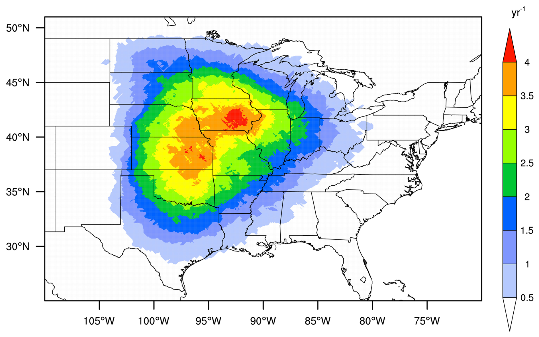
Figure 9 Spatial distribution of yearly averaged annual derecho numbers (ISD-based) over the United States east of the Rocky Mountains between 2004 and 2021. Here, we use derecho areas as the derecho spatial coverage.

6.1 Annual statistics

Figure 8 displays the annual derecho numbers from 2004 to 2021. There is an apparent jump in the derecho number before (∼10 derechos per year) and after 2007 (∼15 derechos per year), which may be partially related to the general increase in the number of gust speed observational sites from 2004 to 2010 (Fig. S5). Figure 9 shows the spatial distribution of yearly averaged annual ISD-based derecho numbers between 2004 and 2021. The central Great Plains has the most frequent derecho occurrences, extending to Oklahoma in the south, Iowa in the north, Kansas in the west, and Illinois in the east. The areas with frequent derecho occurrences are generally consistent with previous studies (Coniglio and Stensrud, 2004; Guastini and Bosart, 2016; Johns and Hirt, 1987; Ashley and Mote, 2005; Squitieri et al., 2025b), although some differences are identified. For example, several studies identified a remarkable northwest–southeast axis with frequent derecho occurrences extending from southern Minnesota to Ohio, which is observable but not apparent in our spatial distribution (Johns and Hirt, 1987; Coniglio and Stensrud, 2004; Guastini and Bosart, 2016; Squitieri et al., 2025b). The differences can be caused by many factors, such as distinct derecho definitions and observational datasets used in these studies. When we used SED gust reports in derecho detection, the spatial distribution of derecho counts showed a more noticeable northwest–southeast axis but with lower derecho numbers than the ISD-based dataset (Fig. S6).

6.2 Monthly statistics

Figure 10 displays the yearly averaged seasonal variations in the derecho count, with remarkably more derechos in the warm than cold seasons, a feature consistent between ISD- and SED-based datasets and widely captured by previous studies (Ashley and Mote, 2005; Squitieri et al., 2023, 2025b; Bentley and Sparks, 2003). However, our dataset has almost no derechos in the cold seasons, which is generally not the case in previous studies except for that of Squitieri et al. (2025b), which also used physically based criteria to detect derechos. We thus attribute the absence of cold-season derechos to our usage of a physically based derecho definition, which excludes many externally forced convective systems (e.g., extratropical cyclones), which have been considered serial derechos in previous studies.

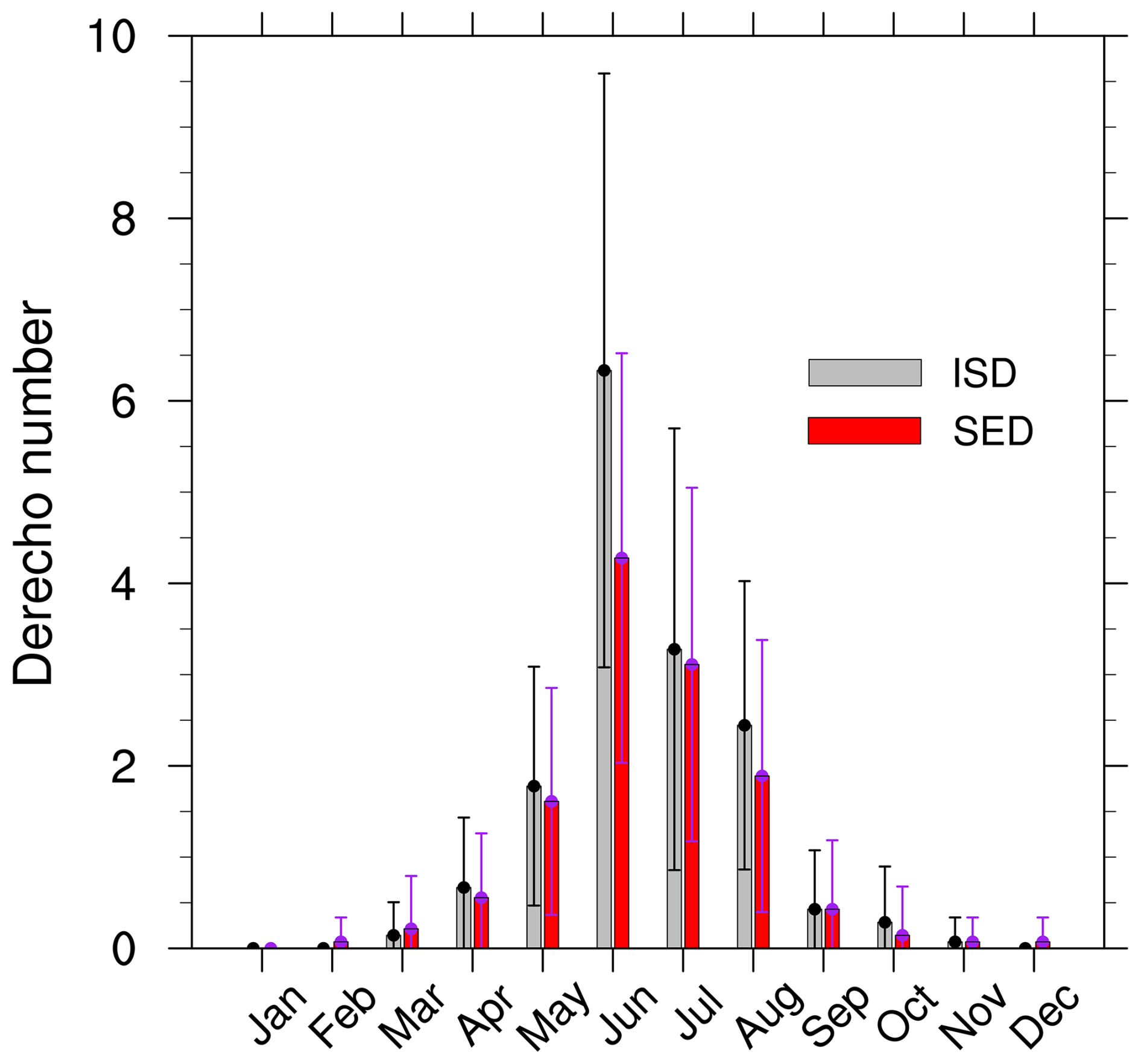
Figure 10 Yearly averaged monthly variations in the derecho numbers between 2004 and 2021. The error bars denote standard deviations. The gray color indicates ISD-based derechos, and the red color indicates SED-based derechos.

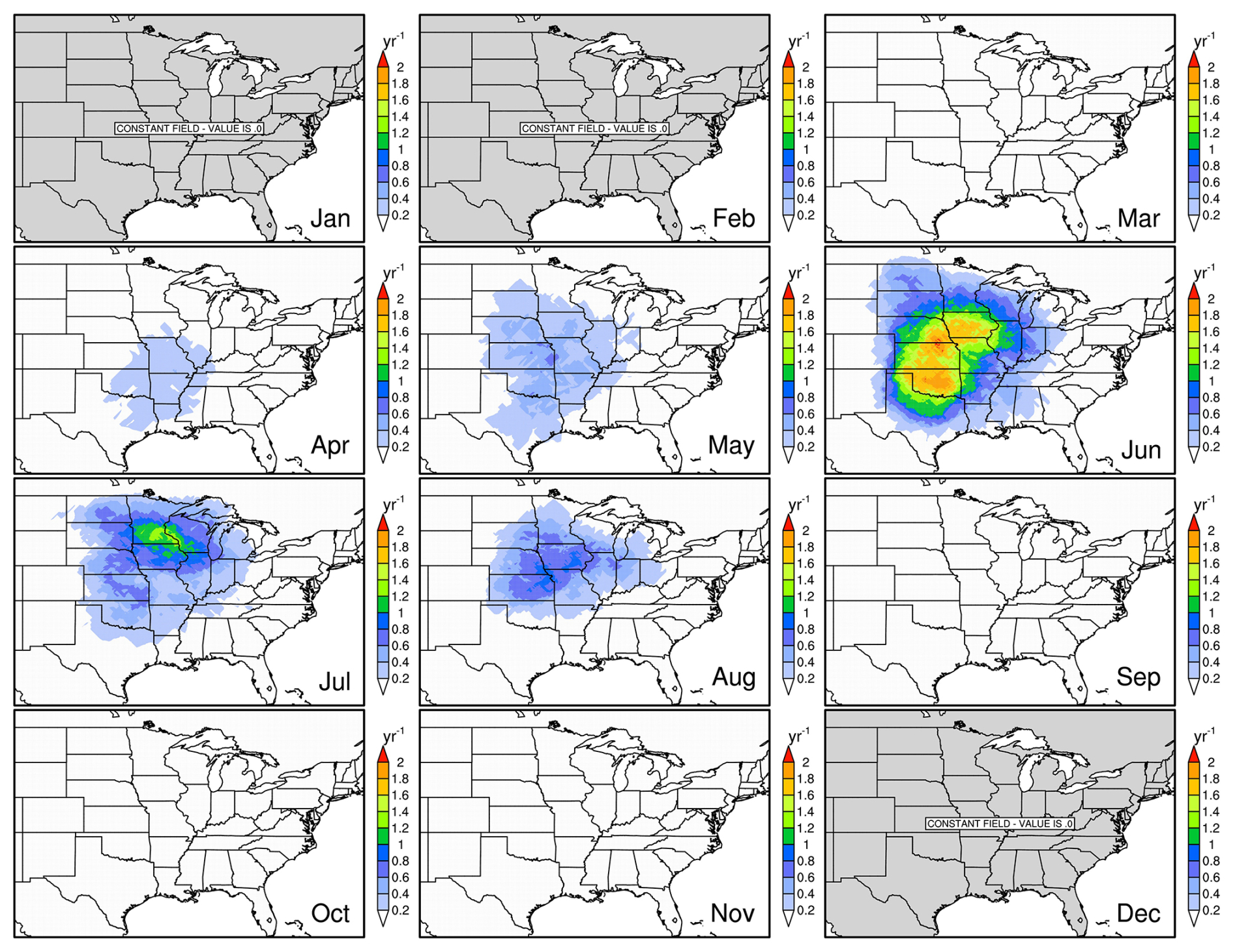
Figure 11 Same as Fig. 9 but for yearly averaged monthly derecho numbers (ISD-based) over 2004–2021.

Figure 11 shows the spatial distributions of the monthly-mean derecho counts based on ISD between 2004 and 2021. On the one hand, many more derechos occur in the warm than cold months. On the other hand, we find remarkable shifts in the areas with the most frequent derecho occurrences from April to August. The region with the most derechos moves northward during the warm season. The northward shifts resemble the MCS events (Li et al., 2021). We can identify two axes with frequent derecho occurrences. One is in the south–north direction along the Great Plains (e.g., June), and the other is in the west–east direction along the northern Great Plains and Midwest (e.g., July). The axes may represent two distinct types of progressive derechos associated with different large-scale meteorological patterns. The SED-based dataset shows similar features but with far fewer derechos in June (Fig. S7).

6.3 Wind damage characteristics

We examine the contributions of DMCSs and derechos to ISD damaging gust reports in the United States within our dataset from 2004 to 2021 (Figs. 12, S2, and S8). Notably, damaging gust reports associated with a DMCS include those from the corresponding derecho as well as those falling outside the derecho location or time window. Overall, MCSs account for about 15.6 % of all damaging gust reports, with the vast majority occurring east of the Rocky Mountains. On average, DMCSs contribute 4.0 % and derechos contribute 3.1 % of all damaging gust occurrences. This indicates that about one-quarter of the damaging gusts associated with MCS events are linked to DMCSs, which is much higher than the fraction (∼3.5 %) of DMCSs in MCSs. This finding aligns with the higher probabilities of extreme gusts in the gust speed probability density function of DMCSs compared to general MCSs, indicating that DMCSs are more likely to produce extreme gusts than general MCSs (Fig. S9). Understanding the mechanisms behind their contrast will be a key focus of a follow-up study. Additionally, approximately 75 % of DMCS-associated damaging gusts occur during the derecho period, reinforcing the validity of our derecho definition. As expected, the highest contributions of derechos to damaging gust reports are found in the Great Plains and Midwest (Fig. 12).

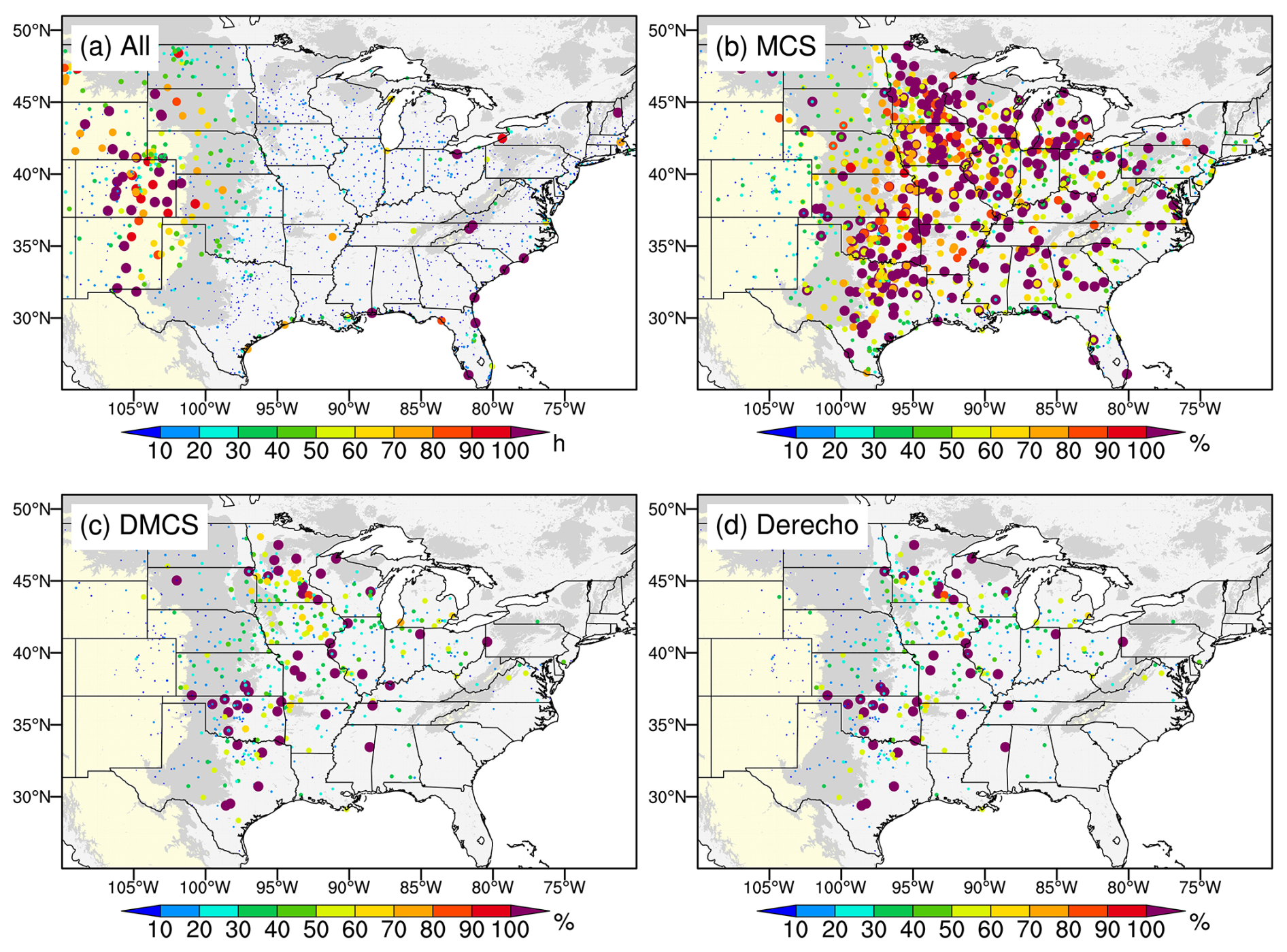
Figure 12 (a) The total numbers of damaging gust occurrences between 2004 and 2021 at ISD weather stations over the United States east of the Rocky Mountains. (b) Relative contributions of MCS events to the damaging gust occurrences in (a). Panel (c) is the same as panel (b) but for relative contributions of DMCSs. Panel (d) is the same as (c) but for derechos. Similar to Fig. 5, we exclude non-derecho-producing MCS events overlapping with TCs in panel (b). The dot sizes are proportional to the corresponding values. Light-yellow shading denotes an elevation greater than 1000 m; light-gray shading denotes an elevation between 400 and 1000 m; and smoke-white shading denotes an elevation less than 400 m. The white background denotes oceans and lakes.

7 Data availability

The final ISD-based and SED-based derecho and DMCS dataset, along with the corresponding user guide, is publicly available at https://doi.org/10.5281/zenodo.14835362 (Li et al., 2025). The dataset is stored in NetCDF-4 format and compressed by year for easier access. The user guide provides a detailed description of the data files, ensuring that users can effectively navigate and utilize the dataset.

For each pair of derecho and DMCS, the dataset includes two visualization figures (one for the derecho and one for the accompanying DMCS) illustrating the temporal evolutions of Z_Hmax, precipitation, wind speed, and gust speed throughout their respective lifetimes (e.g., Figs. 13 and S10). These figures offer users an immediate understanding of the basic characteristics of each derecho and DMCS. The dataset also contains all the derecho-associated gust speeds and various parameter values used in the derecho definition. This allows users to further categorize derechos by intensity or type, following approaches similar to Coniglio and Stensrud (2004).

For researchers interested in applying the segmentation CNN for bow echo detection in different regions or time periods or in leveraging the CNN-identified bow echoes for other studies, we provide access to the bow echo segmentation code and datasets at https://doi.org/10.5281/zenodo.10822721 (Geiss et al., 2024). This repository includes the trained CNN weights and detailed usage instructions. Additionally, a video supplement demonstrating the bow echo segmentation scheme is available at https://youtu.be/iHWY_OhaVUo (Geiss, 2024) and is permanently archived in the above Zenodo repository.

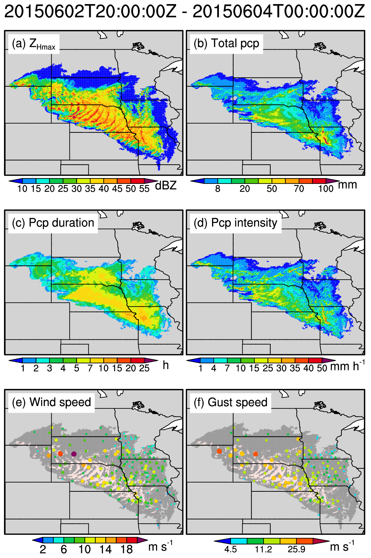
Figure 13 Similar to Fig. 1 but for the spatial evolutions of (a) Z_Hmax, (b) total accumulated precipitation, (c) precipitation duration, (d) mean precipitation intensity, (e) hourly maximum wind speed, and (f) hourly maximum gust speed for an ISD-based DMCS that occurred on 2–4 June 2015. In (e) and (f), the misty-rose shading corresponds to areas with Z_Hmax≥40 dBZ and the dark-gray shading refers to DMCS coverage with Z_Hmax<40 dBZ. The figure title refers to the DMCS timing range.

8 Conclusions

This study presents a high-resolution (4 km and hourly) observational derecho dataset covering the United States east of the Rocky Mountains from 2004 to 2021. We developed the dataset using a combination of an MCS dataset generated by PyFLEXTRKR, bow echoes identified by a semantic segmentation CNN, hourly gust speed data from ISD or SED, and physically based derecho identification criteria.

We evaluated the dataset and its potential uncertainties. The final dataset identifies 274 derechos using ISD gust measurements and 220 derechos using SED gust reports, with most events occurring in the warm season (April–August). Analyses indicate that derechos preferentially occur in the Great Plains and Midwest, with regions of highest frequency shifting northward from April to August. Derechos contributed 3.1 % of ISD land-based damaging gusts over the United States between 2004 and 2021. Additionally, approximately 20 % of MCS-associated damaging gusts were produced by derechos.

As the first derecho dataset that integrates machine-learning-based bow echo identification, physically based definition criteria, and two types of surface gust speed data, the dataset serves as an independent reference for derecho climatology, complementing previous studies. Beyond climatological analyses, the dataset can be used to investigate derecho initiation and development mechanisms, examine the environmental conditions that promote derecho formation and intensification, assess the impacts of derechos on human safety and property, and select specific events for case studies or to evaluate the numerical model simulations, thanks to its high spatiotemporal resolution.

Lastly, we emphasize that the automated derecho detection algorithm developed in this study is versatile and applicable to both observations and model results. The algorithm can be used to assess model performance and explore the impact of various factors on derechos (Kaminski et al., 2025).

Appendix A

For each bow echo in the derecho bow echo series, we used the formulas from the MATrix LABoratory (MATLAB) “regionprops” function (https://github.com/SBU-BMI/nscale/blob/master/original-matlab/features/regionprops.m, last access: 28 January 2025) to calculate its orientation. Then we applied the 3σ rule to the orientations to remove outliers until all the rest of the orientations lay within 3 standard deviations of their mean. The mean is the average bow echo orientation. Implementing the 3σ rule aims to minimize the adverse impact of the segmentation CNN identification uncertainties on calculating the averaged bow echo orientation.

The bow echo series' propagation direction and speed were calculated as follows. Firstly, we computed the moving direction and speed between any two consecutive bow echoes from the series. As exemplified in Fig. A1, we assumed that the bow echo at time t₁ would move to the location of bow echo $t_{\mathrm{1}}^{\prime }$ at time t₂ if the bow echo shape remained unchanged. The location of bow echo $t_{\mathrm{1}}^{\prime }$ was determined by its spatial correlation coefficient with bow echo t₂, and the location with the largest spatial correlation coefficient was what we wanted. Since bow echoes t₁ and $t_{\mathrm{1}}^{\prime }$ have the same shape, it was straightforward to calculate the moving direction and speed between them, which were considered the moving direction and speed between bow echoes t₁ and t₂. Compared to using the centroid points of bow echoes t₁ and t₂, our approach can reduce the calculation bias when bow echoes t₁ and t₂ have distinct shapes and sizes. After we obtained all the moving directions and speeds between any two consecutive bow echoes, we applied the 1.5 × interquartile range (IQR) rule to remove outliers, considering potential CNN bow echo identification errors. Lastly, the median of the remaining moving speed values was considered the bow echo series' propagation speed, while the average of the remaining move direction values was considered the bow echo series' propagation direction.

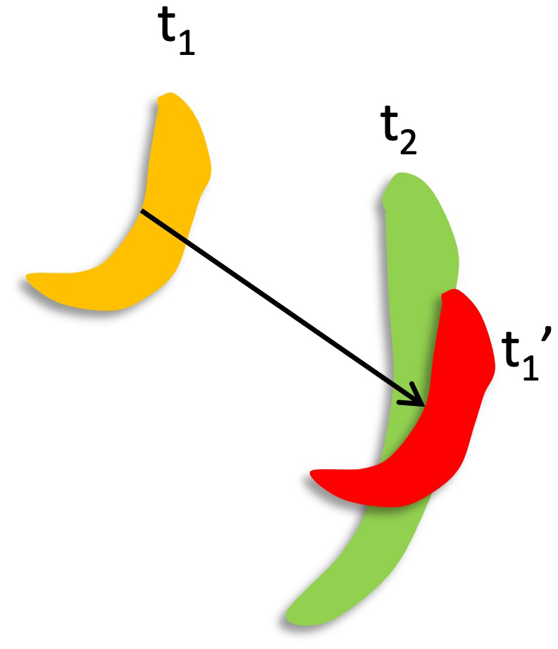
Figure A1 Schematic of the bow echo moving direction and speed calculation between two consecutive (t₁ and t₂) bow echoes. Bow echo $t_{\mathrm{1}}^{\prime }$ is the same as bow echo t₁ but at a different location so that the spatial correlation coefficient between bow echoes $t_{\mathrm{1}}^{\prime }$ and t₂ reaches the maximum. The moving direction and speed between bow echoes t₁ and $t_{\mathrm{1}}^{\prime }$ are considered the moving direction and speed between bow echoes t₁ and t₂.

We used wind speeds at 500 hPa from ERA5 to compute the background mean wind speed. Considering the potential spatiotemporal variability of 500 hPa winds, we only counted wind speeds covered by bow echoes from the bow echo series during the corresponding period. In detail, at time t_i during the bow echo series period (t₁−t_n), we only considered winds at time t_i that were covered by bow echoes from time t_i+1 to $\min (t_{i+\mathrm{3}},t_n)$. Here, we excluded the bow echo at time t_i to minimize the potential impact of the bow echo on the background environment, while using up to 3 h ($t_{i+\mathrm{1}}-t_{i+\mathrm{3}}$) of bow echoes aims to reduce the potential spatial noise since a bow echo is often too small. We averaged all wind speeds obtained from the above procedure to derive the background mean wind speed.