CAMELS-FR dataset: a large-sample hydroclimatic dataset for France to explore hydrological diversity and support model benchmarking

Over the last decade, large-sample approaches, i.e., based on large catchment sets, have become increasingly popular in hydrological studies. Efforts were made to assemble and disseminate national catchment datasets. This article aims to make a contribution to the construction of a large international database of catchments by proposing the CAMELS-FR dataset, a contribution to the CAMELS (Catchment Attributes and MEteorology for Large-sample Studies) initiative. The first version presented here gathers hydroclimatic data and physical attributes for a set of 654 catchments in France. These catchments cover a wide spectrum of hydroclimatic conditions (from oceanic to continental, mountainous, or Mediterranean conditions) and are considered to have limited human influence. Data include time series of daily streamflow (with at least 30 years over the 1970–2021 period, also aggregated to monthly and yearly time steps) and of 11 catchment-scale daily climate variables (including precipitation, potential evaporation, and air temperature), as well as a total of 255 catchment attributes organized into 10 classes (e.g., geology, soil, land cover). River flow time series were quality-checked. Along with the database itself, two graphical tools are proposed, namely dynamic graphs to visualize time series and graphical fact sheets to summarize the main catchment characteristics. Care was taken to provide as many metadata as possible to help users interpret their results based on this dataset. We intend to update the database regularly to include new available data and account for end users' feedback. CAMELS-FR (Delaigue et al., 2024c) is available at https://doi.org/10.57745/WH7FJR.

1 Introduction

In the early days of hydrological modeling, access to data, followed by computing resources, was a major limiting factor of progress, and many of the scientific articles of that time reported results obtained for a single catchment (and sometimes using only a few flood events). The precursors of modern hydrological models were conscious that this was a major shortcoming. Linsley (1982, p. 15) for example recommended that “because almost any model with sufficient free parameters can yield good results when applied to a short sample from a single catchment, effective testing requires that models be tried on many catchments of widely differing characteristics, and that each trial cover a period of many years.” Roughly 20 years later, under the tireless leadership of John Schaake, the so-called MOPEX dataset started to be used worldwide (Schaake et al., 2006), breathing new life into the hard drives of data-thirsty modelers. The paper published by Gupta et al. (2014) 10 years later presented an already impressive list of 94 “large-sample” studies focusing on rainfall-runoff modeling, which had used a dataset of more than 30 catchments. Today, the number of such studies would probably be multiplied by 10, and it has become almost impossible to keep track of all of them. Obviously, computing time difficulties and data sharing possibilities have completely changed.

In France, there has been a long tradition of working with large datasets, following the recommendations of two French leading hydrologists of the 20th century: Maurice Pardé and Marcel Roche. Later, however, large datasets were sometimes mocked as “hydro-bulimia” (Andréassian et al., 2009), and during a certain time, the academic world favored the production of individual basin monographs rather than modeling studies involving large datasets. Over the last decade, progress has been made towards automation of the production (and the updating) of large catchment datasets. In collaboration with the main data producers of hydrometric and meteorological data, we worked to produce the reference hydrological dataset that we present in this paper. For the selection of this dataset, we used what we considered to be “high” quality standards, and because we do acknowledge that there is some subjectivity in this, let us paraphrase Ghislain de Marsily's comment on model validation and state that we strove to do “our level best” (de Marsily et al., 1992) using a variety of automatic data verification procedures, which were complemented by manual checks (including a time-consuming – but clearly necessary – visual data inspection).

With this work, we wish to contribute to the general effort to provide large hydroclimatic datasets as was done in the United States of America (Newman et al., 2015; Addor et al., 2017), Canada (Arsenault et al., 2016), Chile (Alvarez-Garreton et al., 2018), Great Britain (Coxon et al., 2020), Brazil (Chagas et al., 2020; Almagro et al., 2021), Australia (Fowler et al., 2021), central Europe (Klingler et al., 2021), Africa (Tramblay et al., 2021), Denmark (Koch, 2021; Liu et al., 2024), Switzerland (Höge et al., 2023), Saxony (Hauffe et al., 2023), and Germany (Loritz et al., 2024), with many others that will follow. As a national dataset, CAMELS-FR should also be seen as complementary to other datasets built at larger scales that include France, e.g., the EStreams dataset at the European scale (do Nascimento et al., 2024a, b). CAMELS-FR differs from such datasets in the criteria used in the catchment selection process, the data analysis methods, and the choices in data sources that may be available at national but not larger scales.

Before moving to the presentation of the dataset, let us warn the reader that for reasons of scientific ethics, we refused to exclude hydrological “outliers” (i.e., catchments that exhibit unusual hydrological behavior, such as karstic catchments, groundwater-dominated catchments fed by the chalk aquifer of the Parisian Basin, and those with very high baseflow indices) from the CAMELS-FR dataset. We did so because we believe that the outliers are part of the “natural hydrological diversity” (Andréassian et al., 2010) and also because, from a scientific point of view, even good-looking catchments can turn into a “modeler's nightmare” (Refsgaard and Hansen, 2010). This is why we kept, for example, the karstic catchments which have been excluded from other datasets. Note that other catchment sets at the national scale already exist in France for more specific purposes, for example the Reference Low Flow Network to study the long-term evolution of low flows (see Giuntoli et al., 2013; Hodgkins et al., 2024) and elsewhere (see a review of large-sample studies in Gupta et al., 2014).

2 French physical and hydroclimatic context

2.1 Physical characteristics

Metropolitan France (see Fig. 1) covers an area of 550 000 km², including mainland France (spanning 1000 km from north to south and 1000 km from east to west) and Corsica, the fourth-largest Mediterranean island (8700 km²). It is mainly bounded by coastlines (with the North Sea, the English Channel, the Atlantic Ocean, and the Mediterranean Sea) and shares terrestrial borders with eight neighboring countries (Belgium, Luxembourg, Germany, Switzerland, Italy, Monaco, Spain, Andorra). Metropolitan France offers a wide variety of natural landscapes inherited from several geological phases, giving rise to ancient (e.g., Armorican Massif, Massif des Vosges, and Massif Central) and younger mountain ranges such as the Jura, Alps, and Pyrenees (see Fig. 2a). The average altitude is 344 m, and the elevation reaches a maximum of 4806 m at Mont Blanc (in the Alps). These mountain ranges form the boundaries of several sedimentary basins, including the Aquitaine Basin in the southwest and the Paris Basin to the north.

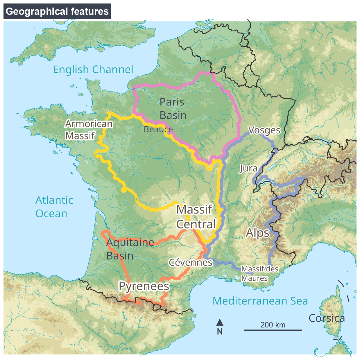
Figure 1 Map of the main geographical features of France: mountain ranges (text with white outline), regions (text without outline), and main basins (pink: Seine; yellow: Loire; orange: Garonne; purple: Rhône) (river network: Lehner and Grill, 2013; digital terrain model, DTM: Lehner et al., 2008; shoreline and political boundaries: Wessel and Smith, 1996; NOAA, 2017).

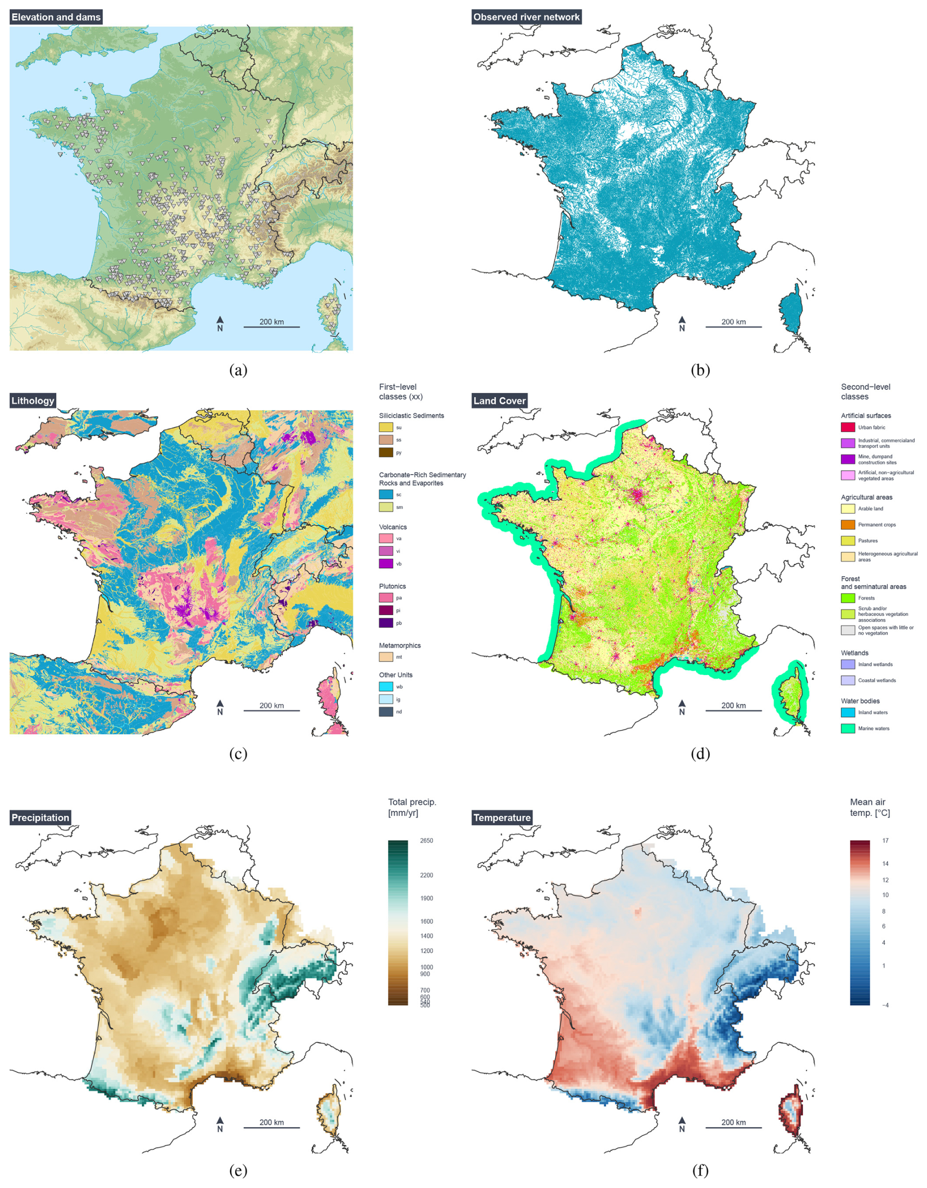
Figure 2 Maps describing metropolitan France territory. (a) Elevation, main rivers, and main dam locations (triangles) (river network: Lehner and Grill, 2013; DTM: Lehner et al., 2008; shoreline and political boundaries: Wessel and Smith, 1996; NOAA, 2017); (b) observed river network (CARTHAGE: French water agencies, 2017b); (c) lithology (GLiM v2.0: Hartmann and Moosdorf, 2012a, b; su: unconsolidated sediment; ss: siliciclastic sedimentary rocks; py: pyroclastics; sc: carbonate sedimentary rocks; sm: mixed sedimentary rocks; va: acid volcanics; vi: intermediate volcanics; vb: basic volcanics; pa: acid plutonics; pi: intermediate plutonics; pb: basic plutonics; mt: metamorphics; wb: water bodies; ig: ice and glaciers; nd: non-defined); (d) land cover (CLC: French Ministry of the Environment, 1990); (e) mean annual total precipitation over the 1991–2020 period (SAFRAN: Quintana-Segui et al., 2008; Vidal et al., 2010); (f) mean air temperature over the 1991–2020 period (SAFRAN).

The French geological diversity is illustrated with the wide range of colors found on the lithological map of France (see Fig. 2c). We give here a short description of the (complex) geology of France, focusing on its implications for understanding the hydrogeology of French catchments. A more detailed account is provided by Pelletier (2021).

• A quarter of France is covered by basement rocks that are metamorphic or igneous in origin. Basement formations host small local aquifers, but no large-scale aquifers. The two main areas are the Armorican Massif in the northwest, almost exclusively composed of ancient formations, and the Massif Central in the center of the country (a more complex area where Hercynian basement, sedimentary formations and recent volcanic formations coexist). Basement rocks also outcrop in smaller massifs of lesser extent (e.g., the Massif du Morvan in the upper Yonne basin, the Massif des Albères at the border of France and Spain in Catalonia, the Massif ardennais around the Meuse River at the border with Belgium, the Massif de la Serre in the Jura Mountains near the Swiss border, and the Massif des Maures on the Mediterranean coast near Saint-Tropez). Note that the Massif des Vosges is divided between basement formations to the south and sedimentary formations to the north.

• Intensely folded areas are hydrogeologically very complex because in these regions, aquifers, if they exist, are of limited spatial extent and therefore difficult to identify for mapping on a regional or national scale. These areas correspond to the most recent massifs: the central and inner part of the Alpine arc, the Pyrenees, and the Languedoc massifs.

• The rest of the territory is occupied by two main types of formations: sedimentary formations and alluvial plains. The sedimentary formations form two major basins: the Paris Basin, which covers a third of metropolitan France, and the Aquitaine Basin in the southwest. Formed by sedimentary deposits left by marine intrusions, they appear as a succession of geological layers with diverse aquifer properties, whose outcrop areas form rings, known as the “pile d'assiettes” (plate stack) in the Paris Basin.

• Alluvial plains and the accompanying aquifers are formed by the scouring and degradation by rivers of various materials, which are then deposited along the river bed. In mainland France, they are generally of limited geographical extent, unlike in other parts of the world. Two alluvial aquifers, however, are of greater importance: they are located in the upper Rhine plain in Alsace and in Bresse (around the Saône River, north of Lyon).

• The variability in surface aquifer properties is clearly apparent when one looks at the density of the observed river network in Fig. 2c, where for example the large areas underlaid by chalk formations in the Paris Basin stand out with their much lower drainage density, while the Champagne Humide region, characterized by clayey and loamy soils, has a much denser river network. The Beauce region, underlaid by the Beauce limestone aquifer complex, is clearly visible as a white spot southwest of Paris, at the border of the Seine and the Loire basins.

In 2015, farmland covered around 51 % of metropolitan France, compared with around 40 % for soils not directly subject to anthropogenic pressures (woodlands, wetlands, and water surfaces) and around 9 % for artificialized soils (see Fig. 2d).

2.2 Hydroclimatic characteristics

According to the Köppen–Geiger climate classification (see, e.g., Peel et al., 2007, and Strohmenger et al., 2024, for a recent analysis of France), more than 90 % of the French territory belongs to the Cfb class (i.e., temperate without dry season and with warm summers), with Corsica and the Mediterranean shore belonging to the Csa and Csb classes (temperate with dry and, respectively, hot or warm summers). The mountain ranges belong to class Dfb (continental without dry season and warm summers), Dfc (continental without dry season and cold summers), and the high-elevation summits belong to the ET class (polar climate). Average annual precipitation ranges from 500 mm yr⁻¹ for the driest regions (e.g., Mediterranean coasts) to more than 2000 mm yr⁻¹ in mountainous regions (see Fig. 2e and f). While precipitation usually varies in a progressive manner over much of the country, a few mountain ranges are characterized by strong differences: one can mention for example the Cévennes range in the south, where average rainfall reaches 2000 mm yr⁻¹, located not far from the Crau lowlands, where average rainfall is less than 500 mm yr⁻¹. A similar situation exists near the Rhine valley in Alsace, where average rainfall in the Massif des Vosges reaches 2000 mm yr⁻¹, while it is less than 500 mm yr⁻¹ in the Colmar plain. As far as temperature is concerned, it is probably enough to mention the mild winter temperatures on the ocean coast and the Mediterranean sea, the lowest temperatures being reached on the high mountain ranges, where a few glaciers still exist despite the global warming trend.

Metropolitan France's hydrographic network (Fig. 2b) is mainly organized around four major rivers (the Loire, Seine, Garonne, and Rhône), whose catchments cover more than 60 % of mainland France. The Rhône and the Garonne catchments are transboundary, with their sources in Switzerland and Spain, respectively. Other transboundary rivers are found in France, such as the Meuse (crossing France, Belgium, and the Netherlands), the Rhine (crossing Switzerland, Liechtenstein, Austria, Germany, France, and the Netherlands), and the Roya (crossing France and Italy), among others (e.g., the Saar, the Oise). The French rivers are characterized by different hydrological regimes, with rain-dominated catchments, both rain- and snow-dominated catchments, snow-dominated catchments, Mediterranean catchments, and groundwater-dominated catchments. The most upstream parts of a few mountainous catchments are still influenced by glaciers. In metropolitan France, glaciers are located in the Alps and in the Pyrenees. Most of them cover rather small areas, especially when related to the area of catchments. The two main glaciers are the Argentière glacier and the Mer de Glace, in the Mont Blanc massif. Vincent et al. (2019) showed that, due to climate change, these two glaciers lost 34 and 45 m of water-equivalent depth, respectively, since the beginning of 20th century, representing 25 % and 32 % of their thickness, respectively. Some other glaciers are located in the Écrins and Vanoise massifs.

Most of France's catchments are impacted by human activities through the presence of large dams (for water supply, hydropower, or flood and low-flow management), river abstraction, and groundwater pumping for agricultural, industrial, and drinking water use; therefore we aimed to exclude the most influenced catchments. The locations of the main French reservoirs are shown in Fig. 2a. Note that a large number of small artificial water bodies exist in France for various uses (recreation, irrigation, boating, fishing, etc.), but often with more limited information available.

2.3 Main data producers

The French hydrosystems have been monitored for several decades through various observational networks, maintained by different organizations. These mainly include national agencies such as Météo-France for climatic data, the French geological survey (Bureau de recherches géologiques et minières, BRGM) for geological and hydrogeological information, the National Institute of Geographic and Forest Information (Institut national de l'information géographique et forestière, IGN) for geographic and forest information, and different state services and independent producers (e.g., EDF, Électricité de France; CNR, Compagnie nationale du Rhône; universities) for hydrological data. These streamflow data are made available by the central service for hydrometeorology and inundation forecasting (Service central d'hydrométéorologie et d'appui á la prévision des inondations, SCHAPI).

3 Catchment boundaries

The first step to build the CAMELS-FR dataset was to delineate the contours of the catchment boundaries, which were then used to calculate hydroclimatic time series at this scale.

3.1 Making a flow direction grid to delineate catchment boundaries at the national scale

Hydrological analysis and modeling require climatic forcing averaged at the catchment scale to be associated with the streamflow measurements recorded at the outlet of a catchment. It was therefore necessary to identify the geographic extent of all French catchments.

To do so, we used a flow direction grid, i.e., a matrix summarizing the topological relationships for metropolitan France. This grid is derived from a topographic analysis of two digital terrain models (DTMs). For continental metropolitan France, we used the DTM from the Shuttle Radar Topography Mission (SRTM) project with a resolution of 100 m × 100 m (Rabus et al., 2003; Farr et al., 2007), and for Corsica, we used the BD ALTI v1.0 from the IGN (2001) with a resolution of 25 m × 25 m.

Because no DTM is error-free, we used an “observed” river network to force the geometry of the theoretical river network to be closer to reality. To constrain the flow directions via the stream-burning method, we used the CARTHAGE river network (French water agencies, 2017b) with removed channels. This method consists of initially burning the vector network in the DTM by artificially lowering the altitude of the pixels belonging to the network. For more details about the method, see Bourgin et al. (2010).

3.2 Geographic repositioning of hydrometric stations on the flow direction grid

When the metadata linked to the gauging stations are well filled in, the geographical coordinates (latitude, longitude, and altitude) and the area of the upstream catchment of the station are available. However, this information is not always consistent with the flow direction grid that we made. Sometimes the resolution of a DTM is not sufficient, and sometimes the gauging station's coordinates are erroneous or not sufficiently precise. Geographically repositioning the hydrometric stations on the calculated flow direction grid is therefore often necessary. Each hydrometric station must be linked with the “river” pixel of the flow direction grid. Only then can the contour and area of the catchment be delineated.

For the gauging stations that are not positioned in a “river” pixel, we searched the theoretical position of the gauging station in the 24 surrounding pixels (i.e., radius of 200 m for continental, metropolitan France) by iteratively calculating the catchment area located upstream of each surrounding pixel. The objective is then to minimize the difference between the area indicated by the data producer (if available) and the area calculated on the flow direction grid. This method allows us to automatically place a large part of the hydrometric stations on the flow direction grid.

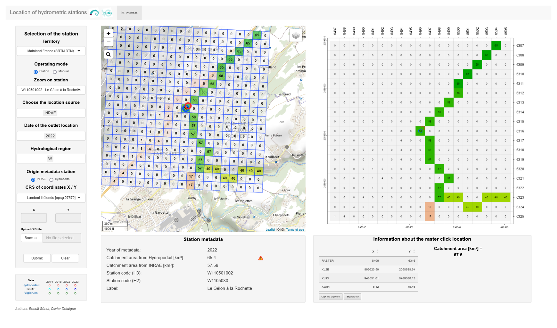
Figure 3 Screenshot of the graphical user interface helping to relocate hydrometric stations in the theoretical river network (Génot and Delaigue, 2018). The left panel is for option selection, where we can select the territory (mainland France or Corsica), a specific station by providing its code or by directly inputting the coordinates, and the metadata year. The middle panel shows the zoomed location of the station on a map layer (“Plan IGN” v2 map layer; IGN, 2020), a superposition of the raster layer with a contributing area grid to aid identification of the correct location of the hydrometric stations. The producer's gauging station is in the red circle, and our own location snapped on the theoretical river network is in the blue circle. The metadata for the searched gauging station are displayed below this map. On the right panel, the contributing area grid and the hydrometric station locations are displayed again, allowing the map to be clicked and the raster information, such as pixel location and its corresponding catchment area, to be extracted.

However, errors still exist at some stations. Therefore, all outlets were checked manually using a graphical user interface (GUI) we developed for this specific goal (Génot and Delaigue, 2018). This GUI (see screenshot on Fig. 3; not made available with the dataset) provides means to analyze the geographical location of the hydrometric station by visualizing maps (e.g., maps or aerial photos) and the comparison between the observed and the theoretical river networks, but also by facilitating the comparison of catchment areas.

4 Selection of the catchment set

The second step to build the CAMELS-FR dataset was to select the catchments based on the following criteria: (i) hydrometric time series availability (Sect. 4.1), (ii) limited influence of artificial reservoirs (Sect. 4.2), (iii) consistency in catchment areas (Sect. 4.3), (iv) sufficient streamflow quality (Sect. 4.4). Starting from 4667 catchments, the successive application of these four selection criteria resulted in sub-sets of 1313, 1055, 1031, and 654 catchments, respectively.

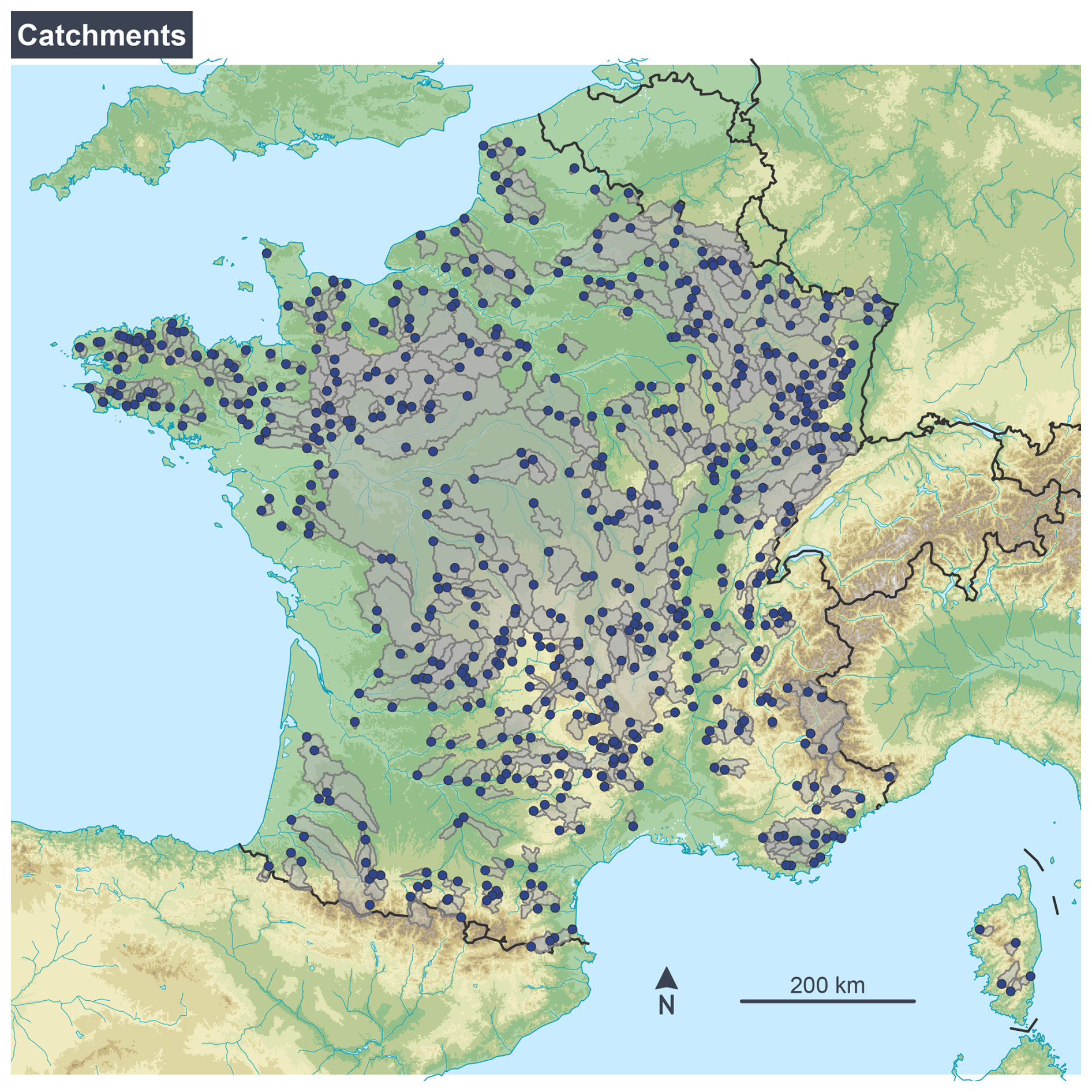
Figure 4 Location map of the 654 catchments and their outlets of the CAMELS-FR dataset v1 (river network: Lehner and Grill, 2013; DTM: Lehner et al., 2008; shoreline and political boundaries: Wessel and Smith, 1996; NOAA, 2017).

4.1 Hydrometric time series availability

We excluded catchments with less than 30 years of complete data over the 1970–2021 period. This record length was arbitrarily chosen because it allows robust statistical analyses. A year was considered complete if less than 20 % of the data were missing.

4.2 Influence of artificial reservoirs

Our objective was to only select catchments displaying a level of human disturbance as low as possible. Here, we only consider influences due to artificial reservoirs. Therefore, the MADAM dataset v1.0 (Delaigue et al., 2024b) was used to estimate these influences. To build this dataset, two sources of information were used, namely the work of Payan (2007) and Payan et al. (2008) and the GEOBS datasets (OFB and partners, 2023), in order to provide locations and volumes of dams in metropolitan France (mainland and Corsica). Each time, we calculated a theoretical level of influence by estimating the equivalent water depth of the total water storage capacity of all dams in the catchment (sum of capacities divided by catchment area).

We cross-checked the two sources of information. The positions of the dams were manually checked. When the storage capacity was inconsistent among the datasets, we validated the dam volume using the website of the French Committee for Dams and Reservoirs (Comité français des barrages et réservoirs, CFBR, 2023), by collecting information from various technical documents of the operators freely available on the internet, or by directly contacting the operators.

Only the catchments with an equivalent water depth of storage capacity lower than 10 mm were selected, thus removing catchments considered highly influenced from our selection. This threshold comes from experience from past studies on this issue (e.g., Payan et al., 2008) but remains arbitrary. The actual level of influence may depend on the local context (location of the dam(s) within the catchment, management objectives of the dam(s), etc.). But we preferred to stick to a single threshold value to have a homogeneous selection criterion.

Note that other types of influence may significantly modify natural streamflow in the selected catchments, typically water withdrawals for various uses or inter-basin water transfers. However, since this information could not be accessed and processed easily, it was not considered here as selection criteria. Thus, the CAMELS-FR catchment set should not be considered to contain strictly non-influenced catchments. For this reason, we also include in the catchment attributes descriptors giving the qualitative estimation of the local and general impact of human influences as provided by the data producers.

4.3 Consistency in catchment areas

The repositioning of the catchment outlets (reported by the data producers, alongside the catchment area) on the flow direction raster was manually checked. We wished to have similar catchment areas between the automatically computed procedure using the flow direction raster and the information provided by the data producers. The catchments whose areas differ by more than 10 % were discarded from the selection. Further investigation would be needed to clarify the reasons for these differences, which may lead to additional catchments in the CAMELS-FR dataset in the coming years. For example, there may exist two types of catchment areas (topographic and hydrogeologic) for karstic catchments in the metadata provided by the producers.

4.4 Streamflow quality inspection

Finally, a visual analysis of streamflow time series was performed in order to identify obvious errors in the streamflow series, such as flow interpolation, sudden drops, and noises not referenced as such. The time series were evaluated by four observers. If at least two observers considered a time series to be incorrect, it was removed from the dataset. If only one observer deemed a time series incorrect, it underwent group re-evaluation to get a consensus on the data quality. Catchments with such errors have been discarded from the dataset, pending data correction from the data producers. This qualitative analysis of streamflow series may lead to the addition (or removal) of catchments in the CAMELS-FR dataset in the coming years. The difficulty of detecting non-natural records in streamflow time series has been recently illustrated and discussed by Strohmenger et al. (2023) on a large set of French catchments.

5 Hydroclimatic time series

5.1 Climatic time series

The SAFRAN atmospheric reanalysis (Quintana-Segui et al., 2008; Vidal et al., 2010) was used as a source of daily climatic time series, aggregated at the catchment scale. SAFRAN is a mesoscale analysis system of near-surface atmospheric variables from the SAFRAN–ISBA–MODCOU hydrometeorological model chain (SIM2; Le Moigne et al., 2020). The SAFRAN data are provided annually by Météo-France at a daily time step from 1958 to the present, and there are no missing data. The reanalysis methodology is regularly updated, and data are updated retroactively (since 1958). SAFRAN uses surface observations combined with data from meteorological models, in particular the ERA reanalysis of the European Centre for Medium-Range Weather Forecasts (ECMWF). Climate variables are analyzed by 300 m altitudinal steps. They are then interpolated on a regular grid with a resolution of 8 km × 8 km (note that catchment rainfall is interpolated from ground measurements). The climatic data cover the whole metropolitan territory (mainland France and Corsica) as well as areas at the borders to correspond to the catchments of rivers flowing into France, with a total of 9892 pixels. An evaluation of the SAFRAN reanalysis is provided in Vidal et al. (2010).

Table 1 List of daily SIM2 variables used in the CAMELS-FR dataset and their aggregation methods at a daily time step.

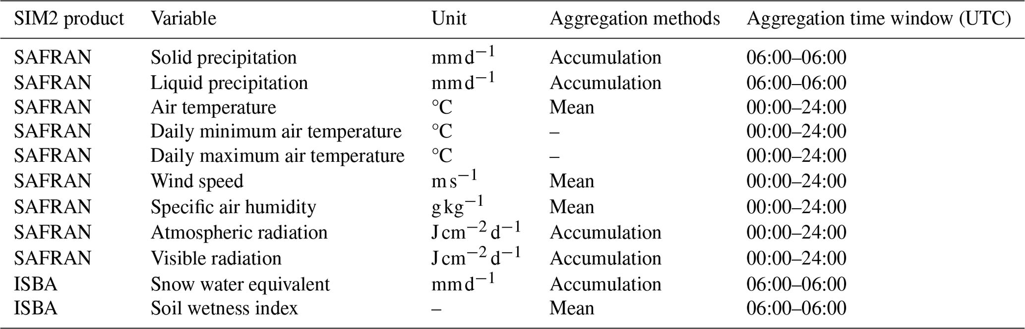
The SAFRAN variables used in the CAMELS-FR dataset are solid precipitation, liquid precipitation, air temperatures (minimum and maximum), wind speed, specific air humidity, and atmospheric and visible radiation. In addition, these climatic data feed a soil–vegetation–atmosphere (SVAT) model called ISBA (Le Moigne et al., 2020) to produce surface variables, such as snow water equivalent and a soil wetness index. Table 1 lists these variables and if they represent daily means or daily accumulations. Note that the aggregation time window may differ between the variables considered, which may have an impact on modeling results.

Using these variables, we calculated (i) three time series of potential evaporation estimates using three commonly used formulas – Penman (Penman, 1948), Penman–Monteith (Monteith, 1965), and Oudin (Oudin et al., 2005) – and (ii) a soil moisture index as computed by the GR4J rainfall-runoff model (Perrin et al., 2003; computed with a reservoir of 275 mm). Note that our versions of the Penman and the Penman–Monteith formulas use a snow-dependent albedo.

The catchment-scale climatic time series are obtained by spatial aggregation of the SAFRAN pixels intersecting the catchment contours. The SAFRAN variables are aggregated at the catchment scale using a weighted average, based on the proportion of pixels within the catchment boundary.

5.2 Hydrometric time series

The SCHAPI (2022) released the Hydroportail application for accessing hydrometric data at the national scale in January 2022. Hydroportail classifies the hydrometric entities into three levels: hydrometric site, hydrometric station, and hydrometric sensor. The hydrometric site refers to a portion of a watercourse on which flows are considered homogeneous. Several hydrometric (gauging) stations can be associated with a single site. A hydrometric station may include several sensors. The main benefit of dividing the hydrometric entities into these levels is to give the producers the possibility of setting a calendar (i.e., periods of validity of each station and sensor) at the site level and to unify the corresponding streamflow data to produce a consolidated time series with a better qualification procedure.

The CAMELS-FR dataset daily streamflow time series were retrieved from the Hydroportail website using the hydroportail R package (Delaigue, 2022). Streamflow data were retrieved at the station level to get all the data, even for sites where calendar information is missing or incomplete. For stations with sub-daily streamflow data, mean daily streamflows are calculated using a trapezoidal method, thus assuming a linear variation in streamflow between successive instantaneous streamflows. This was done directly by the data producer or by the Hydroportail procedure.

Streamflow data are available in the CAMELS-FR dataset in liters per second and were also converted to water depth (in millimeters per day) using the catchment area derived from the DTM (and not producer's area). As climatic data, the streamflow time series are provided at daily, monthly, and yearly time steps.

5.3 Rules for time series aggregation

The time series are provided at daily, monthly, and yearly time steps. For the calculation of monthly time series, a month was considered missing if it had more than 3 d of missing data. The time series at a yearly time step are provided using the hydrological year (considered to start on 1 October) as the basis of aggregation. Therefore the hydrological year of 1970 (first year of the dataset), which starts on 1 October 1969, is deemed incomplete because the first 3 months are missing. Moreover, these yearly data are computed based on the above-mentioned monthly times series. If 1 month is missing, the whole year is considered missing.

6 Catchment attributes

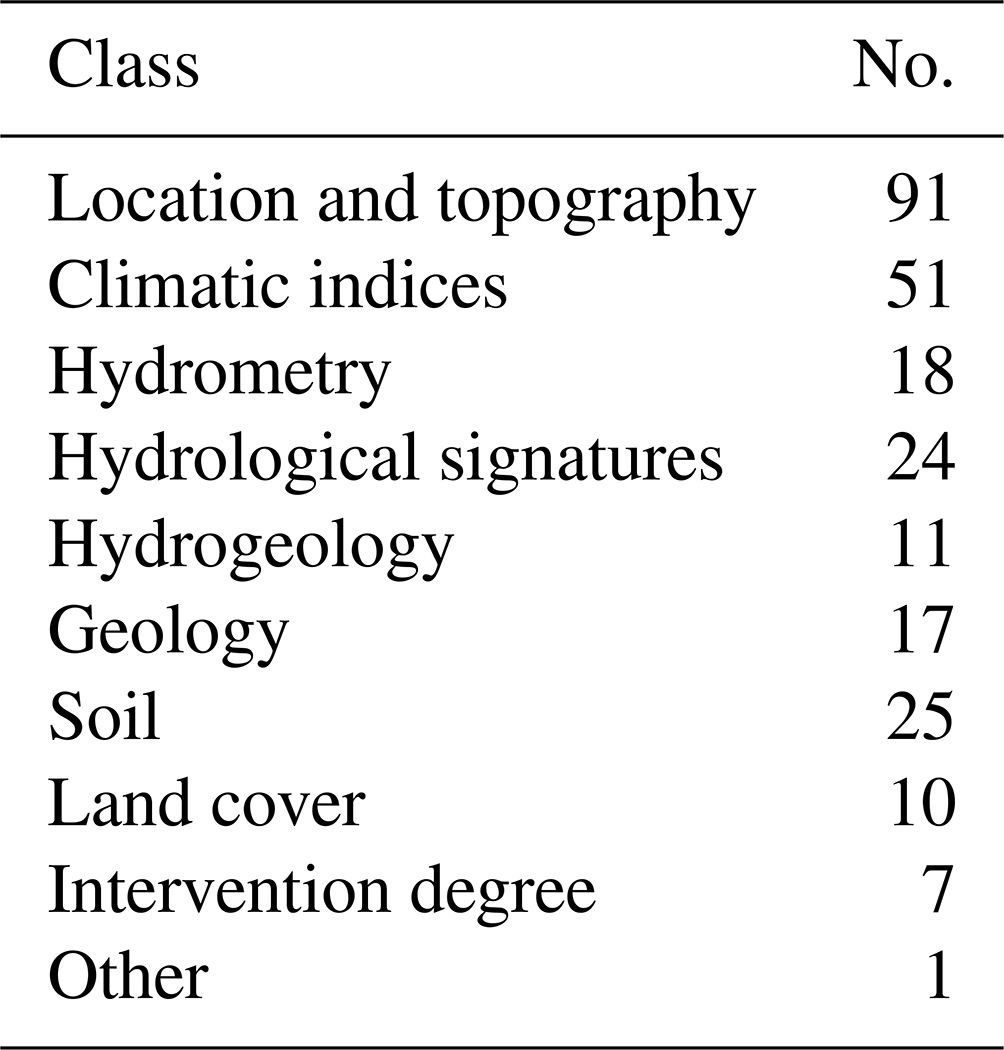
The CAMELS-FR dataset v1 contains 255 attributes, organized into 10 classes (see Table 2), described in the following sub-sections. A spreadsheet listing each catchment attribute is included in the CAMELS-FR dataset.

Table 2 Number of catchment attributes in each class for the CAMELS-FR dataset v1 (the “other” class is related to data access information).

6.1 Location

Most of the location attributes are information given by the data producer and extracted from Hydroportail. Such attributes include the station codes, names, location, type of station, etc. The data producer gives, for most catchments, an estimate of catchment area. Note that for some catchments this area is significantly different from the one derived from the DTM analysis (see Sect. 4.3). Other catchment attributes were computed for the CAMELS-FR dataset. They include station coordinates (after repositioning on the DTM-derived river network), catchment area (derived from the DTM), and information on the station nestedness (indicating whether the catchment is nested, the number of stations downstream, etc.).

6.2 Topography

Two DTMs (NASA and the National Geospatial-Intelligence Agency, NGA, DTM from the SRTM for catchments located on the continent and the BD ALTI v1.0 (IGN) for catchments in Corsica) were used to estimate various attributes describing catchment topography, drainage density, and morphometry. Among the topography attributes are the mean and the percentile distribution for elevation, slope, distance to catchment outlet, and topographic index. The methodology used to calculate the topographic index follows Ducharne (2009), which reformulates the index used in TOPMODEL (Beven and Kirby, 1979) to become a dimensionless index. The percentage of catchment slope classes (flat, gentle, moderate, strong, steep, and very steep) and orientation and the classical drainage density, which is measured as the ratio of total length of stream channels to catchment area (Horton, 1932), are also provided. Among the morphometry attributes, several catchment shape indicators are provided. These include three variants of basin form factor (Horton, 1932; Zăvoianu, 1978, cited by Zăvoianu, 1985, p. 109; Subramanya, 2013, p. 172), the compactness coefficient (Fitzpatrick, 2017), the circularity ratio proposed by Miller (1953) (cited by Zăvoianu, 1985, p. 104), the catchment relief ratio (Fryirs and Brierley, 2013, p. 35), and two variations of elongation ratio: (i) using a circle as a reference (Schumm, 1956) and (ii) using the catchment area as a reference (Fryirs and Brierley, 2013, p. 34).

6.3 Climatic indices

Numerous climatic attributes were estimated: annual mean of different variables (air temperature, potential evaporation, precipitation) over the entire studied period, aridity and seasonality indices, measure of the asynchronicity between the precipitation and potential evaporation, etc. The attributes that use potential evaporation are computed three times using the Penman, Penman–Monteith and Oudin formulas. The attributes of heavy-precipitation-day frequency (frequency of high-precipitation days, i.e., larger than 5 times the mean daily precipitation) and intensity (strongest rainfall on record) and dry-day frequency (average duration of dry periods, i.e., number of consecutive days with precipitation lower than 1 mm d⁻¹) were also computed. Time series of statistics at an annual time step using hydrological year are also provided, including annual daily maximum precipitation and annual seasonality index. As mentioned in Sect. 5.3, the first year (1970) is always missing. Furthermore, maps with a resolution of 1 km × 1 km of hourly and daily rainfall intensity, developed by Arnaud et al. (2008) from the SHYREG-Pluie database (Base de données SHYREG-Pluie ©, INRAE, 2016, all rights reserved), were used to calculate a normalized indicator of rainfall intensity at the catchment scale. This indicator is defined as the ratio of the hourly to daily rainfall intensity with 10-year return period (Poncelet, 2016).

6.4 Hydrometry

Several CAMELS-FR dataset attributes are related to streamflow data quality estimated for each gauging station. Some of these attributes are provided by the data producers. For example, the overall level of uncertainty is qualified by the producer for three flow ranges (high, mean, and low flow). Moreover, several quality codes are assigned to each streamflow value, depending on the way the value was estimated (classical flow estimation using a water level measurement and a rating curve or a value reconstituted a posteriori) (see Sect. 5.2).

Note that this information lacks consistency throughout the CAMELS-FR catchment set, since this qualification is done by regional services, which have different qualification methods according to the regional hydroclimatic context.

Additional attributes were estimated for each station to describe the number of gaps over the studied period (e.g., percentage of missing data in the total period, 1 January 1970 to 31 December 2021) and the overall percentage of streamflow data flagged as questionable or as unqualified by the data producer. A simple algorithm was also applied to identify potential errors due to linear interpolation between two values.

Finally, we attributed to each station an overall estimation of low-flow quality based on the visual analysis of temporal streamflow series: stations with low flows showing suspicious data or behavior have been identified; 52 % of catchments in the CAMELS-FR dataset v1 exhibit such issues.

6.5 Hydrological signatures

As for catchment climate, various hydrological attributes were estimated to describe the main catchment hydrological features. These include catchment aridity (i.e., the ratio of mean daily potential evaporation to mean daily precipitation), catchment yield, streamflow elasticity to precipitation, and catchment seasonality (e.g., month with the minimum mean monthly streamflow). The baseflow index (BFI) was estimated following three different approaches: (i) the method proposed by Ladson et al. (2013) that uses a digital filter, (ii) the method proposed by Gustard and Tallaksen (2008) through linear interpolation of a 5 d non-overlapping streamflow minima (computed with the lfstat R package; Laaha and Koffler, 2022), and (iii) the method proposed by Pelletier and Andréassian (2020) that uses a conceptual quadratic reservoir model (computed with the baseflow R package; Pelletier et al., 2021). For the latter, before calculating the BFI, we filled the gaps in time series with GR6J-CemaNeige (Pushpalatha et al., 2011; Valéry et al., 2014a, b) using the Penman (Penman, 1948), Penman–Monteith (Monteith, 1965), and Oudin (Oudin et al., 2005) formulas. However, we provide the BFI using only the Oudin potential evaporation formula because there were no significant BFI differences when using other formulas. The other attributes that use potential evaporation are computed three times using the three selected formulas. Time series of statistics at an annual time step are also provided for annual maximum daily streamflow and the mean monthly annual minimum streamflow (QMNA) using hydrological and calendar year, respectively.

6.6 Hydrogeology

The average catchment permeability and porosity were estimated thanks to the GLobal HYdrogeology MaPS database (GLHYMPS v2.0) (Huscroft et al., 2018). The national hydrogeological reference map (BDLISA v3) (Brugeron et al., 2018; BRGM, 2022) was used to calculate the karstic portion of the catchments and the percentages of each catchment covered by different hydrogeological formations (e.g., bedrock, sedimentary, alluvial zones).

6.7 Geology

The Global Lithological Map database (GLiM v1.0) (Hartmann and Moosdorf, 2012a, b) was used to characterize the catchment geology. This database, available at a 0.5° spatial resolution, provided estimates of (i) the dominant geological class of each catchment and (ii) the percentages of different lithologies (e.g., metamorphics, carbonate sedimentary rocks; see Fig. 2c).

6.8 Soil

Soil characteristics were described using four datasets. First, the Global 1-km Gridded Thickness of Soil, Regolith, and Sedimentary Deposit Layers v1 produced by Pelletier et al. (2016) was cropped in order to estimate, for each catchment, (i) the mean soil depth and (ii) the distribution (percentiles) of the soil depths over the catchment. The European Soil Database Derived data (ESDD) (JRC et al., 2013a, b) provide soil attributes with a resolution of 1 km × 1 km for a topsoil layer and a subsoil layer with the boundary at 30 cm soil depth for clay, sand, silt, and organic carbon content; bulk density; coarse fragments; and total available water content (TAWC). We therefore, aggregated these two layers from ESDD using the weighted arithmetic mean in cells based on their soil depth for each pixel. We consider the attribute “depth available to roots” to be the correspondent soil depth for each pixel. For the aggregation of TAWC, instead of calculating the weighted arithmetic mean, we calculated the sum of the two layers. Then we cropped the raster for each catchment to extract the percentiles, mean, and skewness of each attribute for the topsoil and the aggregated layer. The EU-SoilHydroGrids v1.0 (Tóth et al., 2017) with a resolution of 250 m × 250 m was used to extract the saturated hydraulic conductivity. This dataset has seven soil layers at 0, 5, 15, 30, 60, 100, and 200 cm depth. The first four layers, which are less than or equal to 30 cm depth, are considered to be topsoil. Therefore, we aggregated these layers to provide information on topsoil (using the first four layers) and the total seven layers as well using depth-weighted harmonic mean. The hydraulic saturated conductivity was divided by 24 in order to provide the results in cm h⁻¹ and then was cropped for each catchment to extract the percentiles, mean, and skewness. Finally, the TAWC was also estimated by INRAE over France from the Réservoir utile des sols de la France métropolitaine v1.2 database (Roman Dobarco et al., 2021; Le Bas, 2021) with a resolution of 90 m × 90 m, providing another distribution of TAWC at the catchment scale.

6.9 Land cover

The CORINE Land Cover dataset was used to estimate, for each catchment, (i) the dominant land cover class and the (ii) percentage of each class on two dates (French Ministry of the Environment, 1990, 2018). This analysis has been performed for all aggregation levels (1, 2, and 3) of the CORINE Land Cover classification.

6.10 Intervention degree

Influence level attributes gather (i) information given by the data producer on the estimated anthropogenic impacts on the observed streamflow time series (four attributes) and (ii) metrics we calculated to estimate the influence of dams present within each catchment (three attributes). Thus, we listed, for each catchment, the number of dams and the total volume of artificial storage.

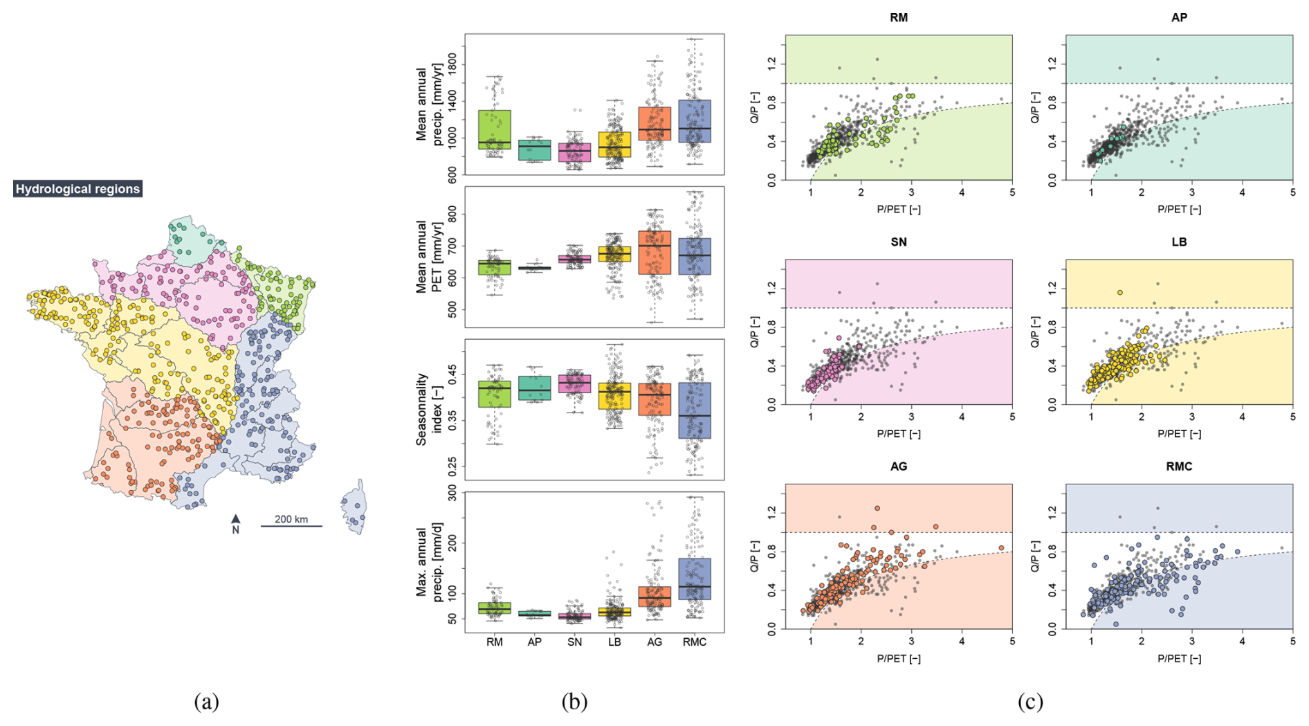
Figure 5 Distribution of CAMELS-FR catchment set over hydrological regions (AG: Adour–Garonne; AP: Artois–Picardie; LB: Loire–Bretagne; RM: Rhin–Meuse; RMC: Rhône–Méditerrannée–Corse; SN: Seine–Normandie; hydrological region boundaries: French water agencies, 2017a): (a) geographical locations, (b) boxplots of climatic indices, (c) projection onto a Budyko-like space (large colored dots: catchments inside the given hydrological region; small gray dots: all the other catchments).

7 Dataset description and add-on products

7.1 Illustration of several attributes of the CAMELS-FR dataset

Figure 5b shows the distribution of four climatic characteristics (mean annual precipitation, mean annual potential evaporation, seasonality index, and maximum annual precipitation) of the CAMELS-FR dataset catchment set, grouped by hydrological region (see Fig. 5a). The northwestern catchments have lower annual precipitation than those in the south, the latter being characterized by high variability in annual precipitation and also in mean annual potential evaporation. Southern catchments show lower seasonality index values, due to Mediterranean climate characterized by a winter maximum for precipitation and significant summer drought (de Lavenne and Andréassian, 2018). Figure 5c shows each CAMELS-FR dataset catchment in a Budyko-type nondimensional space (Andréassian and Perrin, 2012) and for each hydrological region, showing the diversity of hydroclimatic context. Several catchments are located over the water limit (Q=P) or under the energy limit ($Q=P-PET$) due to potential misestimation of precipitation, potential evaporation, or streamflow; errors in catchment area estimation; or non-conservative catchment behavior.

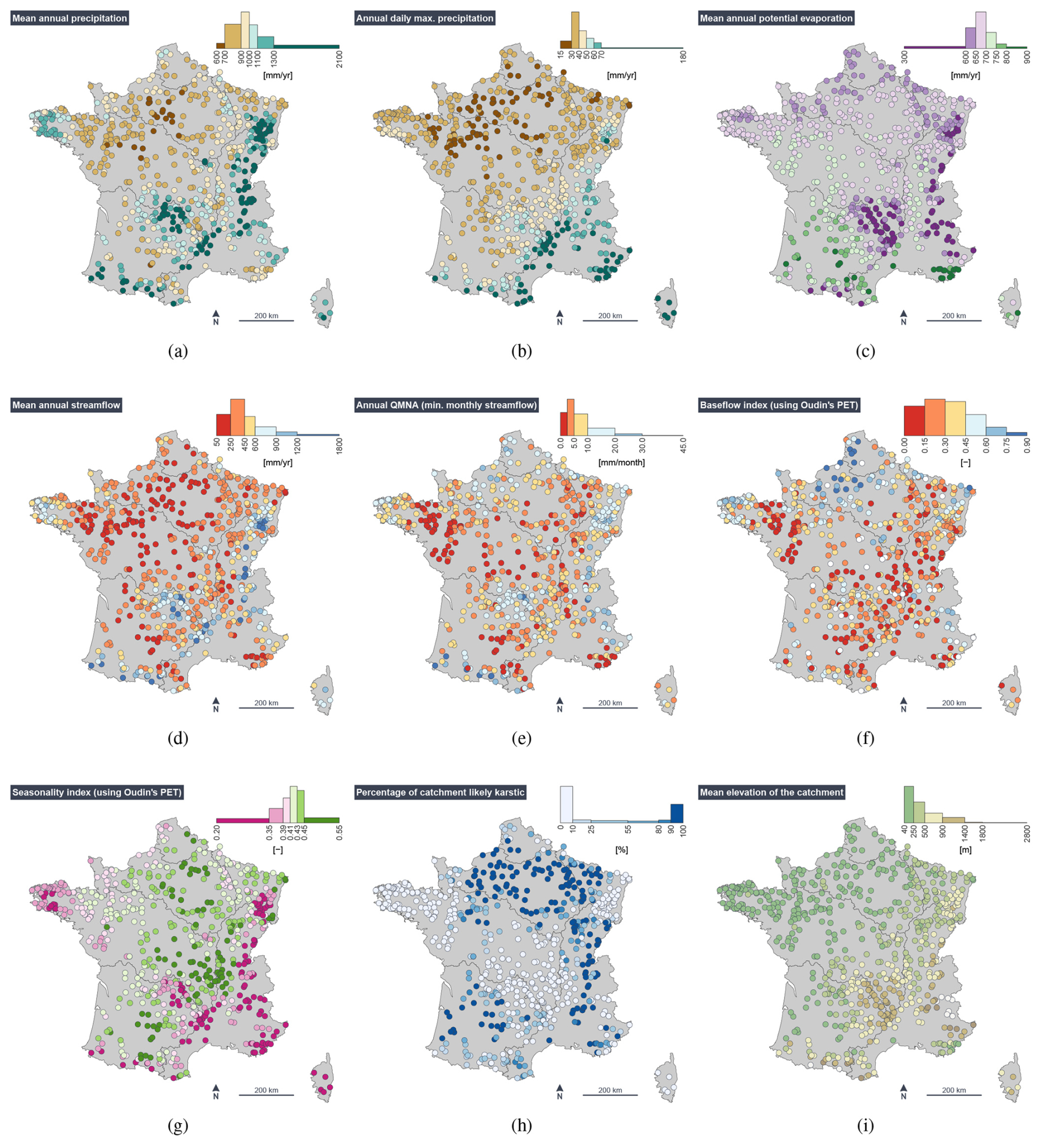
Figure 6 Maps and distributions of a few catchment-scale attributes (hydrological region boundaries: French water agencies, 2017a). (a) Mean annual precipitation, (b) mean annual daily maximum precipitation, (c) mean annual long-term potential evaporation (Oudin method), (d) mean annual streamflow, (e) mean annual minimum monthly streamflow (QMNA), (f) baseflow index using Pelletier and Andréassian (2020), (g) seasonality index (de Lavenne and Andréassian, 2018), (h) percentage of catchment that is likely karstic, (i) mean elevation of the catchment. Note that for those indices requiring a potential evaporation estimate, we consistently used the Oudin method.

Figure 6 presents maps and distributions of three climatic attributes (mean annual precipitation, mean annual potential evaporation, and seasonality index). One can clearly identify the regions with higher-than-average mean precipitation (Fig. 6a): Brittany in the west and all the mountain ranges (i.e., Vosges, Jura, Alps, Massif central, and the Pyrenees). Note that the spatial distribution of extreme precipitation shows a clear structure along a northwest–southeast axis (Fig. 6b), while potential evaporation is structured along a north–south axis, with some variations induced by the mountain ranges (Fig. 6c). Streamflow-related indices (Fig. 6d–f) do not show clear large-scale patterns because they reflect the complex interplay between the climatic factors and the pedo-lithologic factors (see Fig. 2b and c).

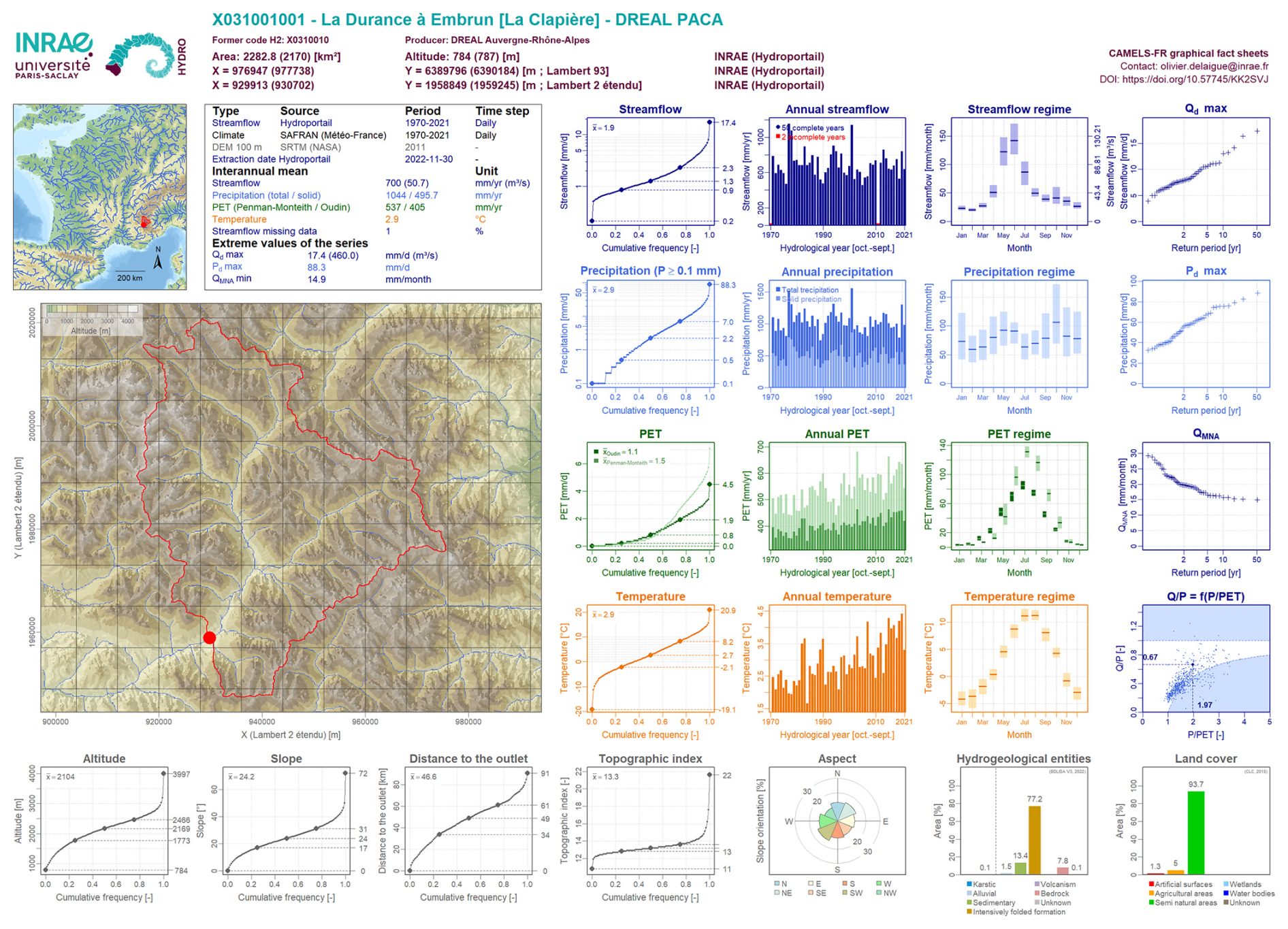
Figure 7 Example of CAMELS-FR graphical fact sheets (Delaigue et al., 2024a) for the X031001001 station (“La Durance á Embrun (La Clapière) – DREAL PACA”).

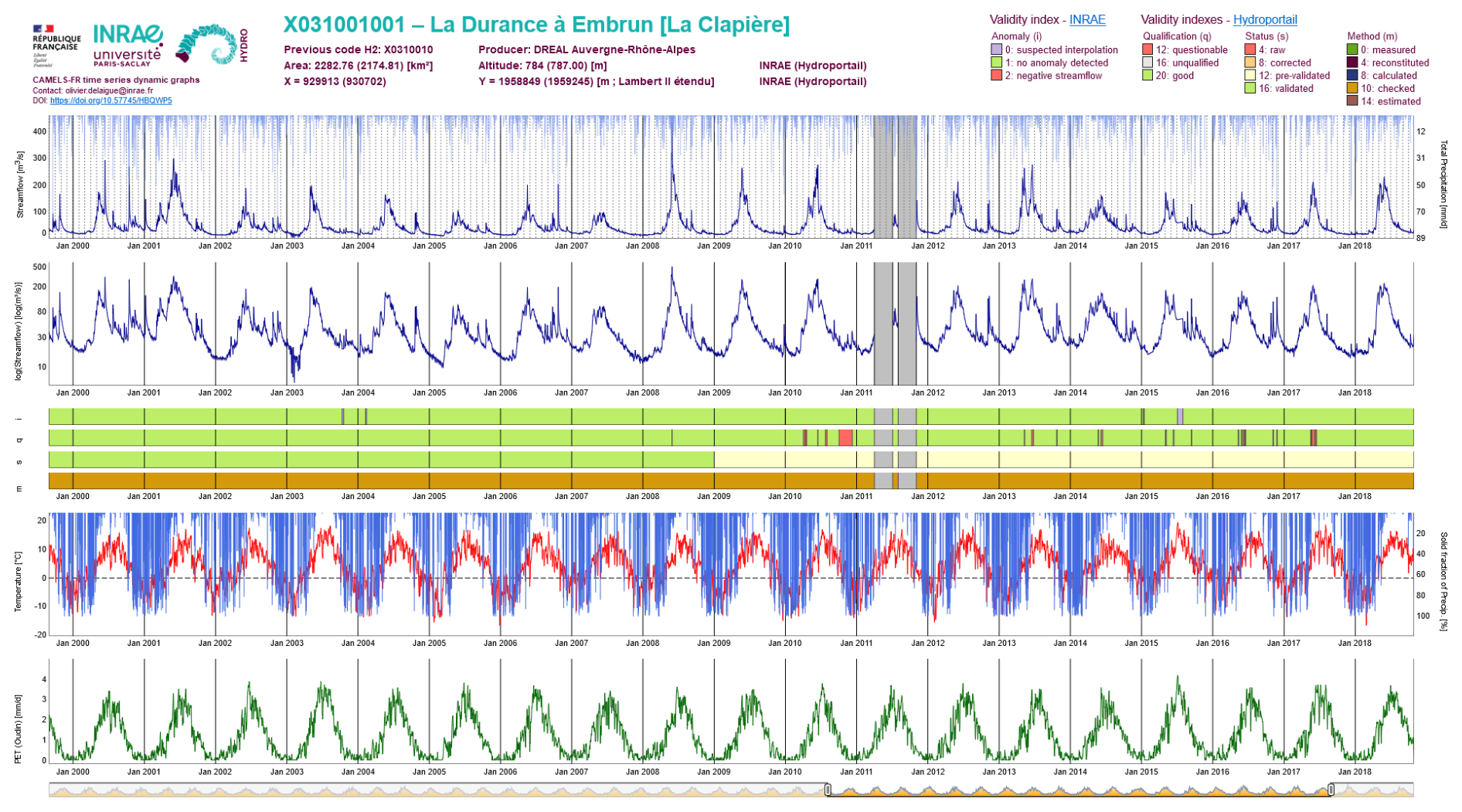
Figure 8 Example of CAMELS-FR time series dynamic graphs (Delaigue et al., 2024d) for the X031001001 station (“La Durance á Embrun (La Clapière) – DREAL PACA”).

7.2 CAMELS-FR add-on products

Two side products were developed around the CAMELS-FR dataset, to provide tools to visualize catchment-scale time series and synthetic summaries to give the user a good overview of the data.

• CAMELS-FR graphical fact sheets (Delaigue et al., 2024a): static plots summarizing hydroclimatic, topographical, hydrogeological, and land cover data (available in English and French) (see example Fig. 7);

• CAMELS-FR time series dynamic graphs (Delaigue et al., 2024d): HTML pages with dynamic plots of hydroclimatic time series (click-and-drag zooming and “onmouseover” display of legends and values; available in English and French) (see example Fig. 8).

8 Data availability

The CAMELS-FR dataset (Delaigue et al., 2024c) can be freely downloaded from the French governmental research data warehouse (https://entrepot.recherche.data.gouv.fr/, last access: 4 April 2025) using the following digital object identifier: https://doi.org/10.57745/WH7FJR. The CAMELS-FR time series dynamic graphs (Delaigue et al., 2024d) and the CAMELS-FR graphical fact sheets (Delaigue et al., 2024a) also have their own digital object identifier, https://doi.org/10.57745/KK2SVJ and https://doi.org/10.57745/HBQWP5, respectively. Most of the variables included in the dataset are based on the French State Open License version 2.0 (https://www.etalab.gouv.fr/licence-ouverte-open-licence, last access: 23 October 2024), which is compatible with the CC BY license. A few are based either on CC BY licenses version 3.0 or 4.0 or specific licenses (provided with the dataset). The CAMELS-FR dataset is distributed under the CC BY license version 4.0 (https://creativecommons.org/licenses/by/4.0, last access: 23 October 2024). Each modification to the dataset can be tracked, as the version number will be automatically updated. Older releases will remain available, even if the data have been updated. A “NEWS” file will be updated in order to track changes between versions.

9 Conclusions and perspectives

The CAMELS-FR dataset v1 gathers data over 654 catchments located in France, including daily hydroclimatic time series over the 1970–2021 period and 255 attributes split into 10 classes (see Table 2). These catchments represent a significant diversity of hydroclimatic contexts (e.g., snow- or groundwater-dominated catchments, Mediterranean catchments). The catchment selection was based on four criteria: (i) streamflow data availability over the 1970–2021 period, (ii) limited artificial influences (quantified based on upstream dam storage only), (iii) consistency between catchment area provided by the data producer and estimated by the DTM analysis, and (iv) visual analysis of the streamflow time series (at a daily time step). We did not consider any selection criteria based on hydrological model efficiency.

The CAMELS-FR dataset was designed to be a “living” dataset. Several changes and updates are planned in subsequent versions: time series lengthening, streamflow value correction by the data producers, addition of “new” catchments (e.g., from French overseas territories). Versions with data at finer temporal and spatial resolutions may also be developed. A web app devoted to the selection of catchment subsets using hydroclimatic, topographical, hydrogeological, or land cover criteria is currently under development. A CAMELS-FR dataset extension to the world-wide Caravan initiative (Kratzert et al., 2023) is also foreseen.