the Creative Commons Attribution 4.0 License.
the Creative Commons Attribution 4.0 License.
 | 26 Mar 2025
Revised and updated geospatial monitoring of 21st century forest carbon fluxes
Melissa Rose
Giacomo Grassi
Joana Melo
Simone Rossi
Viola Heinrich
Nancy L. Harris
Earth observation data are increasingly used to estimate the magnitude and geographic distribution of greenhouse gas (GHG) fluxes and reduce overall uncertainty in the global carbon budget, including for forests. Here, we report on a revised and updated geospatial, Earth-observation-based modeling framework that maps GHG emissions, carbon removals, and the net balance between them globally for forests from 2001 to 2023 at roughly 30 m resolution, hereafter referred to as the Global Forest Watch (GFW) model (see the “Code and data availability” section). Revisions address some of the original model's limitations, improve model inputs, and refine the uncertainty analysis. We found that, between 2001 and 2023, global forest ecosystems were, on average, a net sink of −5.5 ± 8.1 Gt CO2e yr−1 (gigatonnes of CO2 equivalent per year ± 1 standard deviation), which reflects the balance of 9.0 ± 2.7 Gt CO2e yr−1 of GHG emissions and −14.5 ± 7.7 Gt CO2 yr−1 of removals, with an additional −0.20 Gt CO2 yr−1 transferred into harvested wood products. Uncertainty in gross removals was greatly reduced compared with the original model due to the refinement of uncertainty for carbon removal factors in temperate secondary forests. After reallocating GFW's gross CO2 fluxes into anthropogenic fluxes from forest land and deforestation categories to increase the conceptual similarity with national greenhouse gas inventories (NGHGIs), we estimated a global net anthropogenic forest sink of −3.6 Gt CO2 yr−1, excluding harvested wood products, with the remaining net CO2 flux of −2.2 Gt CO2 yr−1 reported by the GFW model as non-anthropogenic. Although the magnitude of GFW's translated estimates aligns relatively well with aggregated NGHGIs, the temporal trends differ. Translating Earth-observation-based flux estimates into the same reporting framework that countries use for NGHGIs helps build confidence around land use carbon fluxes and supports independent evaluation of progress towards Paris Agreement goals. The data availability is as follows: carbon removals (Gibbs et al., 2024a, https://doi.org/10.7910/DVN/V2ISRH), GHG emissions (Gibbs et al., 2024b, https://doi.org/10.7910/DVN/LNPSGP), and net flux (Gibbs et al., 2024c, https://doi.org/10.7910/DVN/TVZVBI).
- Article
(5563 KB) - Full-text XML
- BibTeX
- EndNote


Land is the most uncertain component of the global carbon cycle (Friedlingstein et al., 2023). The highly dynamic and bidirectional nature of terrestrial carbon fluxes, both spatially and temporally, and the contributions of anthropogenic and non-anthropogenic processes pose unique challenges for monitoring fluxes. Top-down atmospheric observations (e.g., from sensors such as NASA's Orbiting Carbon Observatory) are not precise enough to attribute fluxes to specific drivers, and the current suite of bottom-up approaches for estimating global terrestrial carbon fluxes (Friedlingstein et al., 2023) is based on models that are not fully consistent with each other (i.e., bookkeeping models and dynamic global vegetation models (DGVMs) to estimate anthropogenic and natural fluxes, respectively) (Dorgeist et al., 2024; Walker et al., 2024). An additional complication is that these models separate anthropogenic and natural fluxes from land differently compared with national greenhouse gas inventories (NGHGIs), which are used within climate policy treaties to drive national climate actions (IPCC, 2024). This makes it difficult for models to provide estimates directly relevant to climate policy frameworks and national climate action. Top-down atmospheric approaches do not make this separation, while global estimates of anthropogenic land use fluxes from bookkeeping models (Friedlingstein et al., 2023) are 6.7 Gt CO2 yr−1 higher than aggregate NGHGIs (Grassi et al., 2023). This gap is primarily due to definitional and conceptual differences around what is classified as anthropogenic or natural fluxes from forests (Grassi et al., 2018), with recent studies focusing on reconciling these differences (e.g., Schwingshackl et al., 2022; Grassi et al., 2023). Thus, despite improved data acquisition and advances in modeling capabilities, large uncertainty and variation in estimates of land emissions and sinks remain. Moreover, the spatial distribution of forest emissions and, even more so, forest carbon removals are not well understood, impeding the ability of a range of actors, such as governments, companies, and civil society, to monitor the effectiveness of land-based climate mitigation actions that reduce emissions from forest loss and maintain or increase forest carbon sinks.
To address some of these limitations, Global Forest Watch (GFW) introduced an Earth-observation-based framework and model for estimating forest carbon fluxes globally (Harris et al., 2021) that aligns with calls for spatially explicit approaches for the monitoring of forest carbon fluxes (European Council, 2018; Nyawira et al., 2024; Ochiai et al., 2023; Turubanova et al., 2023). It was designed to fill a gap among existing forest carbon monitoring approaches by combining global forest change maps, benchmark carbon density maps, and other Earth observation data based on the Intergovernmental Panel on Climate Change (IPCC) Guidelines for National Greenhouse Gas Inventories (IPCC, 2006, 2019) that countries use to estimate emissions and removals for their NGHGIs. Within the scope of the Agriculture, Forestry, and Other Land Use (AFOLU) sector, only greenhouse gas (GHG) fluxes from forest-related land uses and land use changes (forest remaining forest, non-forest converted to forest, and forest converted to non-forest) were included. The framework was designed around the United Nations Framework Convention on Climate Change (UNFCCC) guiding principles for NGHGI preparation: transparency, accuracy, completeness, comparability, and consistency. All GFW carbon flux model inputs and outputs and code are publicly available (see the “Code and data availability” section).
Recognizing that both Earth observation and ground data increase and improve through time, we designed GFW's flux monitoring framework and the model implementing it with the flexibility to accommodate updates to existing components and add new components. Here, we document updates to the model, report results from the current version, present a revised uncertainty analysis, and – following the recommendations of the recent IPCC Expert Meeting on Reconciling Land Use Emissions (IPCC, 2024) – introduce a new translation of GFW model of CO2 emissions and removals into NGHGI reporting categories of deforestation and forest land that provides an Earth observation perspective on forest fluxes conceptually similar to what countries are expected to report under IPCC guidelines.
Harris et al. (2021) include a detailed explanation of the GFW forest flux monitoring framework, but some key elements are described here. The framework encompasses gross CO2 emissions from the loss of carbon in aboveground and belowground biomass pools, dead wood, litter, and soil organic carbon in mineral soils due to stand-replacing disturbances; carbon loss from drainage of organic soils; and methane (CH4) and nitrous oxide (N2O) emissions from forest fires and drainage of organic soils. Carbon removals include sequestration into aboveground and belowground forest biomass. All model inputs are resampled to the spatial resolution of a Landsat pixel (0.00025 × 0.00025°, roughly 30 × 30 m at the Equator), and outputs are generated at the same resolution. The model uses the Landsat resolution because it is the highest resolution at which the global forest change maps and an aboveground biomass map for the year 2000 are publicly available. Higher-resolution maps of forest change and biomass exist but are not publicly available, are available only for recent years, and/or include only certain regions (e.g., Vancutsem et al., 2021; Yang and Zeng, 2023).
The IPCC GHG inventory guidelines, the methodological basis of GFW's forest carbon flux monitoring framework, lay out two methods by which terrestrial carbon stock changes associated with land use, land use change, and forestry (LULUCF, part of the broader AFOLU sector) can be calculated: gain–loss and stock-difference (IPCC, 2006). Methods can be applied according to different tiers (from 1 to 3) with increasing complexity and presumed accuracy. In the gain–loss method, carbon emissions and removals are calculated separately by multiplying activity data, such as forest area lost, gained, or maintained (ha), by emission or removal factors (t C ha−1); the net carbon stock change, or flux, is the difference between gross emissions and gross removals. In the stock-difference method, carbon stocks are measured during repeated inventories, and the difference between remeasurements is the estimate of net carbon stock change, or flux. GFW's framework employs the gain–loss approach, in which the activity data and other contextual information are estimated using global Earth-observation-based maps trained on local ground plot data and/or airborne and spaceborne lidar observations.
GFW's gain–loss modeling approach is initialized in the year 2000 with global maps of carbon densities in five forest ecosystem carbon pools (Fig. 1). The model runs for all pixels with a canopy density ≥ 1 % in 2000 (Hansen et al., 2013), but default outputs define forests as follows: (1) > 30 % canopy cover in 2000 (Hansen et al., 2013) or subsequent tree cover gain (Potapov et al., 2022b), (2) nonzero aboveground biomass in 2000 (Harris et al., 2021), (3) mangroves in 2000 (Giri et al., 2011), and (4) exclusion of oil palm plantations in 2000 (see Table 2). We use this definition of forests because a canopy density of > 30 % is a common threshold employed for national definitions of forests (Harris et al., 2018) and because some of the input removal factors are specifically applicable to denser forest. All outputs and results use a canopy density > 30 % unless otherwise specified. However, because the model runs without any a priori canopy density threshold and the forest definition is applied after the fact, fluxes can be estimated for lower canopy density thresholds. Within pixels with canopy cover in 2000, gross removals are mapped based on locations of forest extent and regrowth, while gross emissions are subsequently mapped based on locations of stand-replacing forest disturbances. In this system of tracking the forest/non-forest status of individual pixels over time, the model adheres to IPCC Approach 3 for land representation (IPCC, 2019).
For activity data, rather than combining and reconciling national or regional geospatial forest monitoring data in the limited places where they exist continuously since 2000, we deliberately use global, independent (nongovernmental) data sources to maintain global consistency and comparability within the framework, recognizing that global data are generally not the most locally accurate or relevant data but that they remain useful for large-scale analyses and potentially for verification purposes of other approaches. To identify forest loss, the GFW model uses the Global Forest Change (GFC) data of Hansen et al. (2013), which are updated annually. Because of the framework's use of GFC, emissions are limited to those from stand-replacing disturbances or other disturbances severe enough to be detected by GFC. Tree cover gain (Potapov et al., 2022b) is gross gain and is assigned to the period from 2000 to 2020, not to a specific year. In the model, forest pixels can have loss only (assigned to a specific year), neither loss nor gain (i.e., no change), or both loss and gain (in which the order is unknown). Non-forest pixels can have either tree cover gain or no gain; in the latter case, they are outside the framework, as they are non-forest remaining non-forest.
Emission and removal factors likewise use spatially explicit data as much as possible to capture spatial variation in forest properties and dynamics and move beyond ecozone-level representation of forests. GFW model emission and removal factors are generally independent of national data sources, with the exception of some removal factors in temperate forests, which are derived directly from the Forest Inventory and Analysis (FIA) database maintained by the United States Forest Service (see Harris et al., 2021, and Glen et al., 2024, for details). The model uses a combination of IPCC default (Tier 1) and localized (Tier 2) emission/removal factors, with the goal of using more Tier 2 factors over time, just as countries are encouraged to do in their NGHGIs. (Note that some Tier 1 removal factors come from national forest inventories, particularly FIA data (IPCC, 2019).) For example, removal factors in primary forests use IPCC defaults (Tier 1; IPCC, 2019), while initial (year 2000) aboveground biomass carbon densities use a global benchmark map of woody biomass developed from field data and remote sensing (Tier 2; Harris et al., 2021). Removal factors are applied in a hierarchy from six sources: (1) mangrove-specific rates (IPCC, 2014a); (2) Europe-specific rates by forest type (combination of Table 4.11 of the updated IPCC guidelines, FAO planted forest assessment, and factors published in national forest inventories); (3) planted tree rates from the Spatial Database of Planted Trees (SDPT) Version 2.0 (Richter et al., 2024); (4) US-specific rates by region, forest type, and age class derived from the FIA database (Glen et al., 2024); (5) young secondary forest rates (Cook-Patton et al., 2020); and (6) IPCC default rates for all other areas (e.g., primary forest, older secondary forests in the tropics, and older temperate forests outside Europe and the US) (IPCC, 2019). The framework supports the addition of other geospatial removal factors as they become available. Gross removals are added to pre-disturbance biomass until the year of loss to determine the biomass in the year of loss. Emission factors are estimated using a map of tree cover loss drivers (Curtis et al., 2018) and burned area (Tyukavina et al., 2022); the combination of these determines the extent to which carbon pools (including soil organic carbon in mineral soils) are emitted by forest disturbance. Emission factors are estimated using “committed” emissions (Hansis et al., 2015) or instantaneous oxidation (IPCC, 2019), whereby carbon loss from all relevant pools is assumed to occur in the year of disturbance rather than modeling delayed carbon fluxes through time.
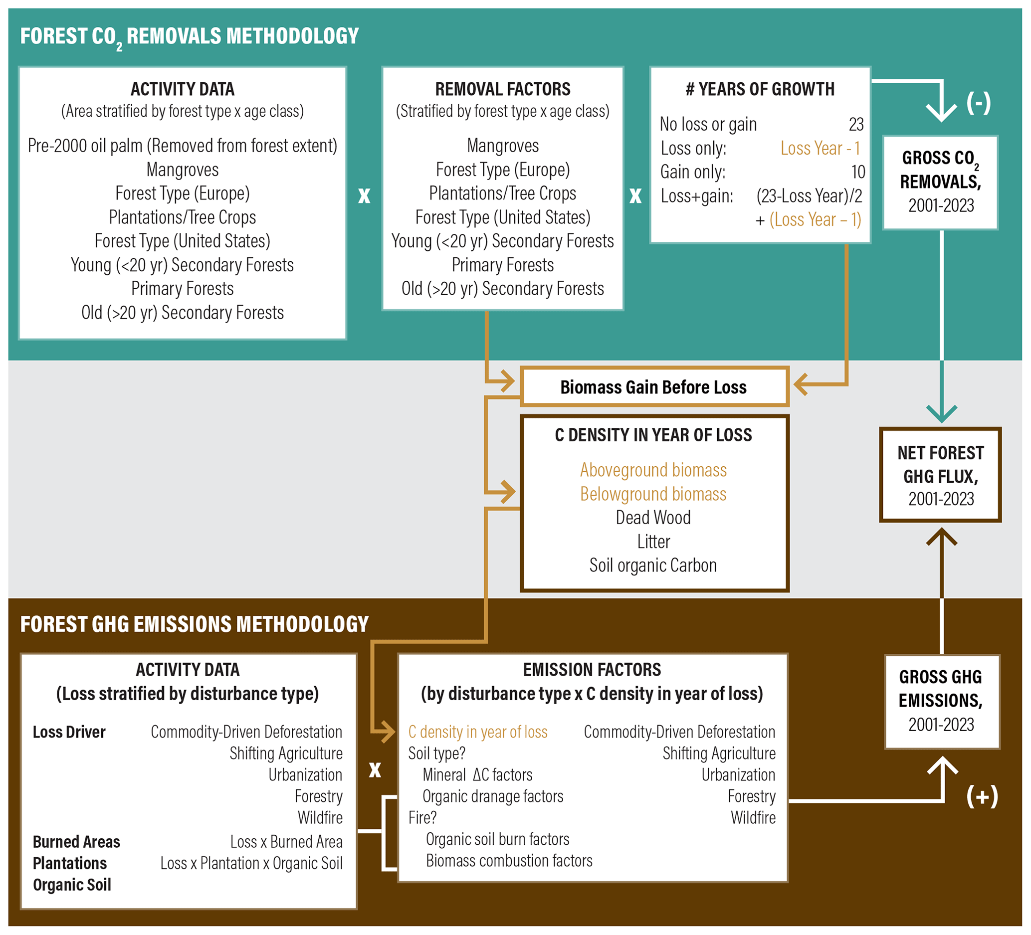
Figure 1Updated conceptual framework for modeling forest-related GHG fluxes. The model estimates gross forest-related emissions and removals as the product of activity data and emission/removal factors for each ∼ 30 m pixel. The net forest GHG flux is the sum of gross emissions (+) and removals (−). Text and arrows in gold are portions of the removals methodology that are passed into the emissions methodology.
2.1 Changes to GFW model input data
Since the original release of GFW's carbon model framework in 2021, which estimated forest carbon flux results through 2019, we have made several changes to the model inputs because new data were published or existing data were improved (Table 1). These changes keep the model aligned with recent advances in global Earth observation data and address some limitations in the original version, but they do not change the underlying conceptual framework. The updated geospatial inputs are shown in the context of all inputs in Table 2. We summarize changes to the input data with respect to extension of the model from 2019 to 2023 (Sect. 2.1.1), changes to activity data (Sect. 2.1.2), and changes to emission and removal factors (Sect. 2.1.3).
Table 1Changes to GFW model inputs since the original version (Harris et al., 2021).
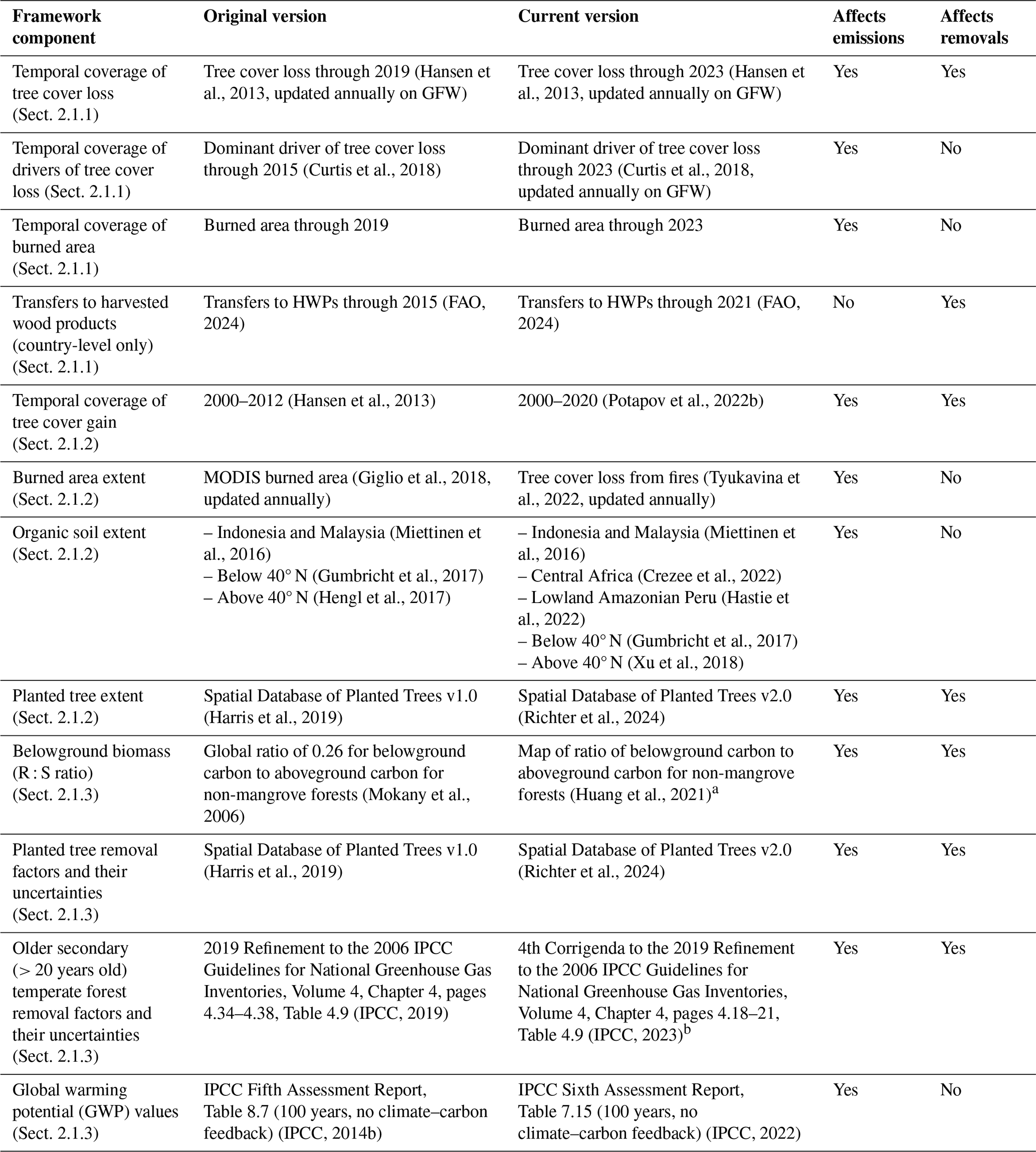
a The R : S ratio map was extended outwards to fill gaps in the original map. b Removal factors for other climate domains and ages were not updated.
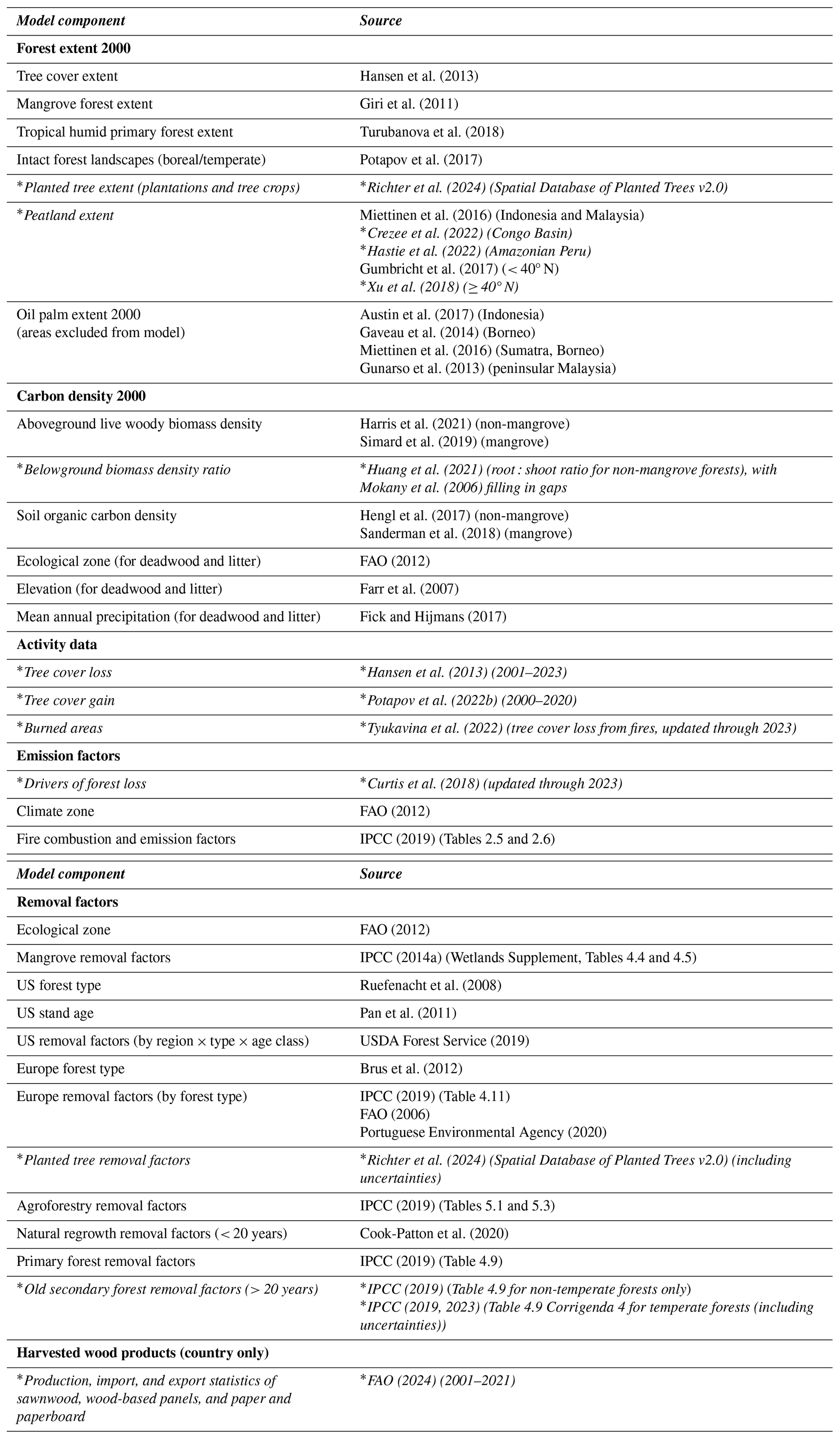
Table 2Geospatial data components and sources currently used in the GFW model. Updated components and sources are denoted using an asterisk (*) and italic font. This updates Table S3 in Harris et al. (2021).
2.1.1 Annually updated data
We have updated four inputs to the framework annually since the original GFW model was published: tree cover loss, dominant driver of tree cover loss, burned area, and country-level transfers to harvested wood products (HWPs). In the original version, they extended to 2019, 2015, 2019, and 2015, respectively. The first three inputs now extend through 2023, and we plan to continue to update them annually, lagging 1 year behind the calendar year. Country-level HWP transfers now extend through 2021 based on data from FAOSTAT that currently extend through 2022 (https://www.fao.org/faostat/en/, last access: 5 May 2024). These constitute the core updates to the model each year.
2.1.2 Updated activity data
Beyond the annual updates described above, we made the following four additional updates to the model's activity data:
-
Temporal coverage of tree cover gain. Tree cover gain originally covered 2000–2012 but now covers 2000–2020. In the original version, tree cover gain covered 7 fewer years than tree cover loss did (12 years of tree cover gain vs. 19 years of tree cover loss); currently, tree cover gain covers 3 fewer years than tree cover loss (20 years vs. 23 years). Tree cover gain is still reported in one interval, so the framework does not assign gain to a specific year within 2000–2020. The shorter duration of tree cover gain and its lack of information on timing is an ongoing limitation of the inputs to the framework (see Sect. 4.3 and 4.4).
-
Burned area extent. The original version of the GFW model used MODIS burned area (500 m resolution) (Giglio et al., 2018), but it now uses Global Land Analysis & Discovery laboratory tree cover loss due to fires (TCLF) (30 m resolution) (Tyukavina et al., 2022). This burned area product is designed to be used with GFC. As in the original version of the model, emissions from fires are included only where stand-replacing disturbances are detected by GFC, meaning that emissions from relatively low severity forest fires remain unquantified in the model.
-
Organic soil extent. We added two new regional tropical peatland maps (Peru and Congo Basin; Hastie et al., 2022; Crezee et al., 2022) and replaced the peat map above 40° N (Xu et al., 2018). These maps reflect a more recent understanding of the extent of organic soils in those regions. This is one of the few inputs to the model that composites regional maps with pan-tropical and global maps.
-
Planted tree extent. Planted trees are part of managed ecosystems, and using distinct removal factors for planted trees instead of removal factors for natural forests better represents the associated carbon sequestration of these managed landscapes. The original version of the GFW model used SDPT v1.0 (Harris et al., 2019), but it now uses SDPT v2.0 (Richter et al., 2024), which includes the planted tree extent in 45 additional countries. Richter et al. (2024) define planted trees as plantation forests and tree crops. This dataset aggregates maps of tree crops and planted forests globally in a bottom-up approach that captures roughly 90 % of the planted tree area globally circa 2020. Each polygon in the database has the most taxonomically resolved information available, from a broad type of production (e.g., orchard) to species.
2.1.3 Updated emission and removal factors
We made the following four updates to emission and removal factors:
-
Belowground biomass (R : S ratio). The original version of the GFW model used a single R : S ratio of 0.26 to estimate belowground biomass applied globally to non-mangrove forests (Mokany et al., 2006). (Mangroves had separate ratios from (IPCC, 2014a).) The updated model uses a global R : S ratio map from Huang et al. (2021) to incorporate spatial variability in the R : S ratio, ranging from less than 0.15 to greater than 0.5. Because the R : S ratio map does not cover all land where forest is present in our framework (e.g., some nearshore islands), we interpolated missing R : S ratio pixels from nearby ones; where interpolation was not possible (e.g., remote Pacific islands), we retained the original default ratio of 0.26. We applied this ratio map to aboveground biomass in the year of tree cover loss to calculate carbon emissions from loss of belowground biomass. We also used the R : S ratio map to calculate carbon removals by belowground biomass based on carbon removals by aboveground biomass. Including this input makes the belowground carbon stocks and removal factors reflect local forest types better than using a single global ratio.
-
Planted tree removal factors and their uncertainties. SDPT v2.0 (Richter et al., 2024) has a removal factor and uncertainty associated with every planted tree (planted forest and tree crop) polygon included in the database. The removal factors of polygons that were in SDPT v1.0 are largely unchanged in SDPT v2.0, but polygons newly included in SDPT v2.0 have been assigned removal factors based on information about what kind of planted tree is present using the most taxonomically resolved information available.
-
Older (> 20-year-old) secondary temperate forest removal factors and their uncertainties. The original version of the framework applied Tier 1 removal factors published in Table 4.9 of IPCC (2019) for primary and some secondary (>20-year-old) temperate forests. In 2023, IPCC released corrected default removal factors and their uncertainties for temperate secondary forests in North and South America, which are also applied in the GFW model to >20-year-old forests in temperate ecozones outside of the USA and Europe where no better sources of data are currently available. In the model update, we replaced the original IPCC defaults with the corrected ones.
-
Global warming potential (GWP) values. The original version of the framework converted non-CO2 emissions from CH4 and N2O into equivalent units of CO2 using GWP values published in IPCC's Fifth Assessment Report. The framework now uses GWP values for CH4 and N2O from IPCC's Sixth Assessment Report. This affects gross emissions and net flux outputs only where non-CO2 emissions are estimated (organic soil drainage, fires in organic soils, or biomass burning).
2.2 Updated uncertainty analysis
With the original version of the framework, we presented an uncertainty analysis that used an error propagation approach for inputs for which uncertainties (variances) were available and potentially substantial. This approach underlies Approach 1 (simple error propagation) outlined in the IPCC guidelines and produces similar results; however, it reflects exact calculations of variances and standard deviations, whereas the IPCC Approach 1 to uncertainty analysis is an approximated approach that yields 95 % confidence intervals (IPCC, 2019). For the model update, we repeated this uncertainty analysis with all of the changes and updates to the framework described in Sect. 2.1, using the same error propagation approach and the same components employed in the original analysis.
2.3 Anthropogenic fluxes from “managed” forests
GFW's Earth-observation-based modeling framework does not (and cannot) differentiate between anthropogenic and non-anthropogenic fluxes from forests. Rather, it includes fluxes from all forest land and, therefore, the combination of direct anthropogenic, indirect anthropogenic, and natural fluxes. Thus, results from our model are not directly comparable with those from NGHGIs or bookkeeping models, each of which define anthropogenic fluxes with different system boundaries for their specific purposes (Grassi et al., 2022, 2023). Under UNFCCC decisions and IPCC methodological guidance, countries report only anthropogenic fluxes in their NGHGIs, approximated by “managed land” (IPCC, 2006; Ogle et al., 2018). Therefore, if GFW's forest carbon flux monitoring framework is to serve as an independent, Earth-observation-based point of reference for NGHGIs, its results must be able to be reported in a conceptually similar way, covering the same scope. In doing so, we adopted the proposal of Grassi et al. (2023), who recommended adjusting global data to the NGHGI framework for analyses focused on country policy or action. In translating the GFW model's fluxes into the NGHGI reporting framework, we did what IPCC guidelines direct countries to do when compiling and reporting their inventories, rather than what countries necessarily do in practice for their inventories. The goal of this translation exercise was not to reproduce as closely as possible how countries prepare their NGHGIs using the GFW model, to achieve maximum quantitative similarity to NGHGIs, or to reconcile the GFW flux model with NGHGIs; rather, we aimed to present CO2 fluxes from a globally consistent, geospatial approach in the same conceptual terms that national policymakers use.
We developed a three-step process to translate the GFW model's gross CO2 emissions and removals into three IPCC reporting categories: anthropogenic flux from managed forest land, emissions from deforestation (anthropogenic), and non-anthropogenic flux from unmanaged forest (Table 3). It builds upon the simpler comparison between the GFW model and NGHGIs conducted in the IPCC Sixth Assessment Report (Nabuurs et al., 2022), in which anthropogenic fluxes from the GFW model were those outside primary forests in the tropics and intact forest landscapes in the non-tropics. This translation process does not change the GFW model's bottom-line net flux estimates; rather, it reclassifies the gross CO2 fluxes by intersecting the GFW model fluxes with other contextual geospatial data to provide fluxes more conceptually aligned with those of NGHGIs. The first step (Sect. 2.3.1) assigned each country to one of three cases based on how their NGHGI applies the managed land proxy (Fig. 2). The second and third steps reclassified the GFW model's emissions (Sect. 2.3.2) and removals (Sect. 2.3.3), respectively, into three IPCC reporting categories according to the three cases assigned in step 1 (Fig. 2). Emissions and removals within each IPCC reporting category were then summed to calculate net anthropogenic and non-anthropogenic forest-related CO2 fluxes for each country. The GFW model calculates annual emissions, corresponding to the year of tree cover loss, but does not calculate annual removals; instead, it calculates removals as an annualized average over the entire model period. Thus, to generate time series from the GFW model using the NGHGI reporting categories, we calculated the average annual removals in each reporting category by dividing gross removals by the number of model years. Therefore, the resulting time series for each reporting category is the difference between the annual emissions for that year and the average removals.
For this analysis, we used data from the GFW model for 2001–2022 to align with the temporal coverage of NGHGIs. We limited our comparison to CO2 fluxes only (i.e., excluding CH4 and N2O emissions from the GFW model) but note that some developing countries do not separately report CO2 and non-CO2 emissions. Because the GFW model cannot currently report emissions from organic soil separately from all other emissions, we combined NGHGIs' deforestation and organic soil emissions (including emissions from forest land, from peat decomposition and peat fires typically associated with deforestation, and from agriculture soils) to achieve the same scope as the model. We excluded transfers into the harvested wood products pool from both data sources in this translation analysis, as that is not a core element of our geospatial framework.
Table 3Translating GFW flux model gross CO2 emissions and removals to national greenhouse gas inventory (NGHGI) reporting categories. To calculate the total net CO2 flux for IPCC reporting categories, GFW flux model emissions and removals were reclassified according to managed land status (managed vs. unmanaged) and driver of tree cover loss. Following IPCC guidelines, for Case 2 countries, we used information about the driver of tree cover loss to reassign initially delineated unmanaged forest to managed forest where direct human activity is observed to result in tree cover loss (i.e., forestry; commodity-driven deforestation, CDD; urbanization; and shifting agriculture). Thus, all associated fluxes from unmanaged forests reassigned to managed forests are reported in the corresponding anthropogenic IPCC reporting category (anthropogenic forest land flux and deforestation).
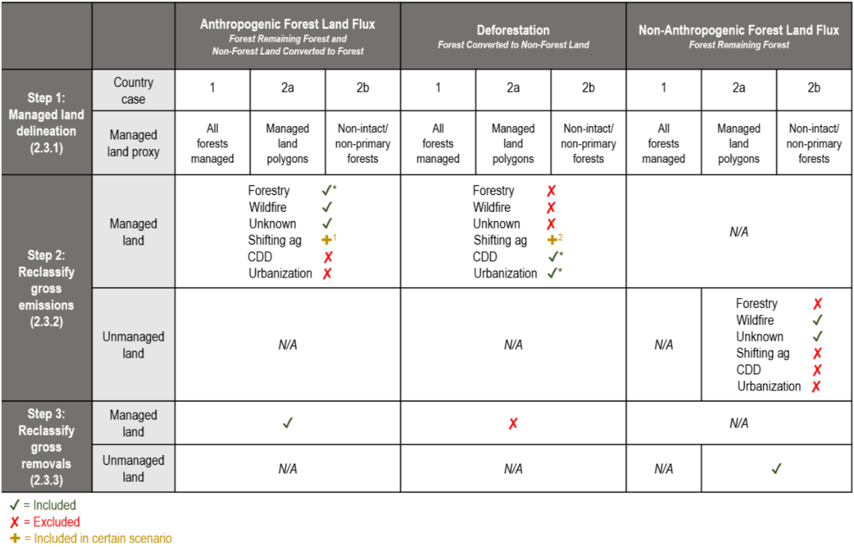
* Includes emissions from not only the initial delineation of managed forests but also from tree cover loss in unmanaged forests reassigned to managed forests due to direct human activity. 1 To calculate the maximum emissions in anthropogenic forest land, we count emissions from shifting agriculture (shifting ag) in secondary forest toward the anthropogenic forest land flux and emissions from shifting agriculture in primary forests toward deforestation. 2 To calculate the maximum emissions from deforestation, we count all emissions from shifting agriculture in both primary and secondary forest toward deforestation. This also corresponds to a larger sink in anthropogenic forest land. N/A denotes “not applicable”.
2.3.1 Managed land delineation
In the first step (top rows in Table 3), we assigned countries to one of three cases based on careful review of NGHGIs and the availability of in-country information on the distribution of managed and unmanaged forests. These cases describe which land is considered managed and unmanaged according to information that countries provide in their NGHGIs regarding their use of the managed land proxy (Fig. 2). Case 1 included 46 countries (primarily UNFCCC Annex 1 countries, i.e., advanced economies with annual GHG reporting commitments) that explicitly consider all forest land managed and another three countries (China, India, and Indonesia) for which we assumed that all forest land is considered managed, based on the information provided in their NGHGIs. Case 2 included all other countries, which do not consider all forest to be managed and, thus, consider some forest to be unmanaged. For the three Case 2a countries (Brazil, the USA, and Canada), we used the georeferenced boundaries of managed and unmanaged lands that they use in their NGHGIs. The remaining 143 countries (UNFCCC non-Annex 1 countries, i.e., countries with historically less stringent GHG reporting commitments) either report no information or not enough details regarding the use of the managed land proxy and its extent. For example, Russia's inventory explicitly includes unmanaged land but reports areas by administrative unit rather than spatially, which is not adequate for our analysis. For these Case 2b countries, we approximated managed forest in tropical regions as forests outside humid tropical primary forests from 2001 (Turubanova et al., 2018) and in extratropical regions as forests outside intact forest landscapes from 2000 (Potapov et al., 2017). For Case 2 countries, the initial managed forest delineation was modified in steps 2 and 3 to include unmanaged land reassigned to managed land due to direct anthropogenic activity. We note that while countries' definitions of forest land differ, we instead used a single, global definition of forest (as defined in Sect. 2): a tree cover density > 30 % (Hansen et al., 2013).
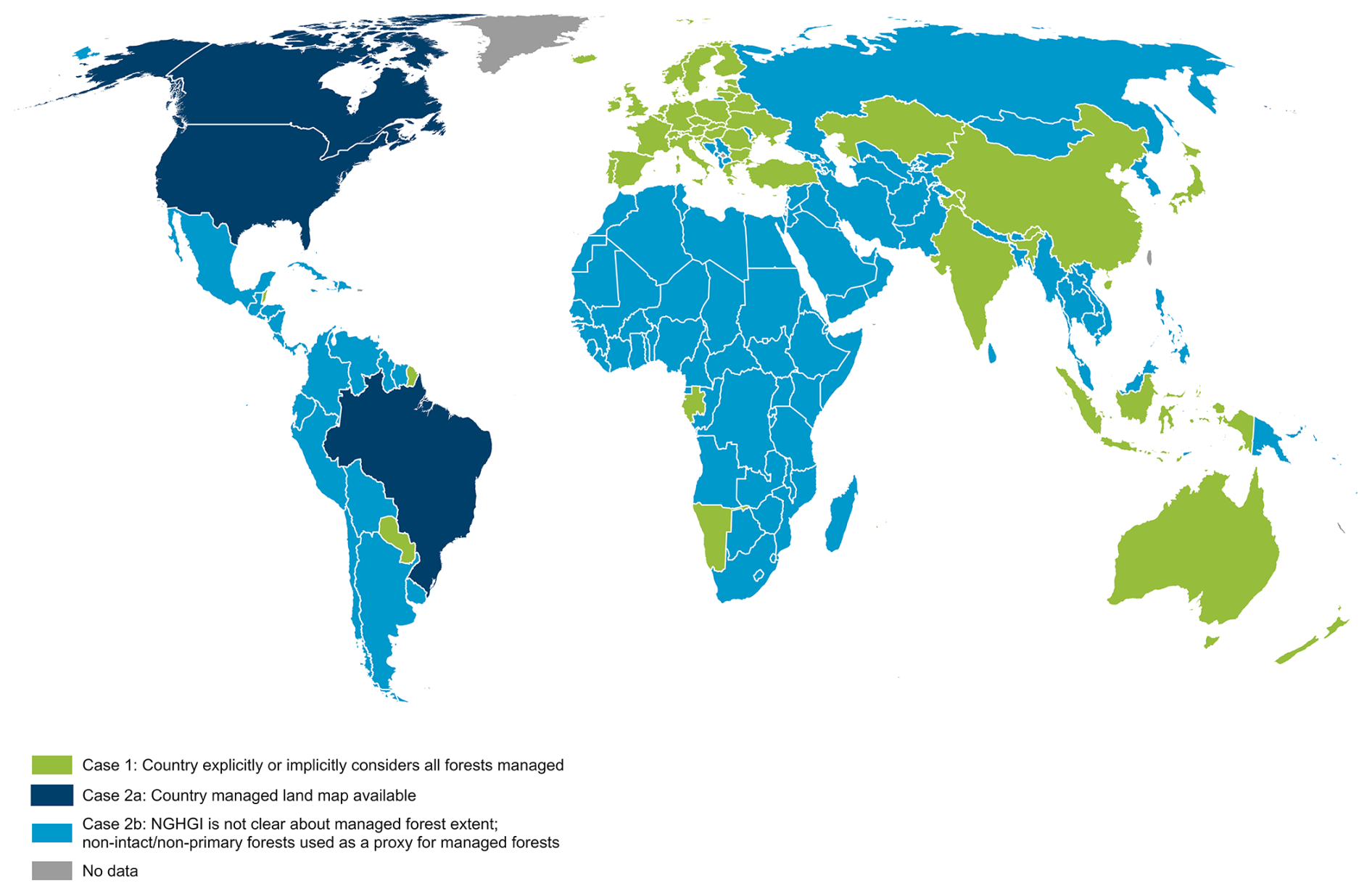
Figure 2Country representation of managed land in their national greenhouse gas inventories (NGHGIs) as of 2024, before transitioning to the Paris Agreement rules, and as interpreted for this study. Countries consider fluxes by forests in several ways in their national greenhouse gas inventories (Melo et al., 2025). Some countries explicitly or implicitly consider all forests to be managed and thus include all forest fluxes in their NGHGIs (Case 1). The rest do not consider all forests to be managed. Only a few countries (Case 2a) use maps of managed lands to delineate anthropogenic fluxes from non-anthropogenic fluxes. The rest are not clear in their NGHGIs regarding the spatial extent to which forests are or are not considered managed and thus which forest fluxes are included in their inventories (Case 2b). Publisher's remark: please note that the above figure contains disputed territories.
2.3.2 Reclassifying gross carbon dioxide emissions
In the second step (middle rows in Table 3), we combined the initial delineation of managed forests described in Sect. 2.3.1 with a map of drivers of tree cover loss (Curtis et al., 2018, updated through 2023) to partition the GFW model's gross CO2 emissions into IPCC reporting categories, as not all of the GFW model's gross emissions are from deforestation. For Case 1 countries, which classify all forests as managed, all emissions occurring within country borders were anthropogenic and no emissions were non-anthropogenic. For Case 2 countries, all emissions within managed forest boundaries (defined in Sect. 2.3.1) were anthropogenic and the remaining emissions within initially delineated unmanaged forest boundaries were either anthropogenic or non-anthropogenic depending on the driver of the tree cover loss. We expanded our definition of managed forests to include initial unmanaged forest (as defined in Sect. 2.3.1) where there is direct human activity, such as forest harvest or deforestation (IPCC, 2006). Thus, we considered all emissions from direct human activity to be anthropogenic. The remaining emissions – from natural or seminatural drivers of tree cover loss, such as wildfire, occurring within unmanaged forest boundaries – were the only emissions that we considered to be non-anthropogenic.
Using this delineation of anthropogenic vs. non-anthropogenic, we reclassified the GFW model's gross emissions into three categories that are conceptually aligned with IPCC reporting categories (Table 3): anthropogenic emissions from managed forest land (“forest remaining forest” plus “non-forest land converted to forest”), anthropogenic emissions from deforestation (“forest converted to non-forest land”), and emissions from unmanaged forest land that are non-anthropogenic by definition (“forest remaining forest”). These categories are outlined as follows:
-
Anthropogenic emissions from managed forest land. For all countries, this category included emissions from wildfire and the negligible emissions not assigned to a driver (Curtis et al., 2018) occurring within managed forest areas. This category also included emissions from forestry regardless of where they occurred (inside or outside of initial delineated managed land boundaries, as defined in Sect. 2.3.1), as harvest activity is a direct human activity and, thus, any tree cover loss from forestry activity results in the reclassification of unmanaged forest to managed forest.
-
Anthropogenic emissions from deforestation. For all countries, this category was the sum of all emissions from tree cover loss due to commodity-driven deforestation and urbanization, regardless of where they occurred, as well as emissions from the loss of intact/primary forests in areas of shifting agriculture, as this is considered a permanent change in land use.
-
Non-anthropogenic emissions from unmanaged forests. For Case 1 countries, we assumed (based on their NGHGIs) that all forests are considered managed and, thus, no emissions are considered non-anthropogenic. The two categories above represent all CO2 emissions from the GFW model for those countries. For Case 2 countries, which have some unmanaged forest (as defined in Sect. 2.3.1), non-anthropogenic emissions were the sum of the remaining emissions outside managed forests – emissions from tree cover loss due to wildfires and the (small) unassigned drivers class (Curtis et al., 2018). Although some fires in unmanaged land can be caused by humans, we classified emissions from them as non-anthropogenic to be consistent with IPCC guidelines; separating emissions from human-caused fires in unmanaged land and reporting them as anthropogenic forest land emissions could be improved in further iterations of this analysis.
It is often not clear which land use categories emissions from shifting agriculture cycles are allocated to in NGHGIs, as this distinction is not required by the IPCC guidelines (IPCC, 2019). Following Curtis et al. (2018), shifting agriculture landscapes are defined as “small- to medium-scale forest and shrubland conversion for agriculture that is later abandoned and followed by subsequent forest regrowth”. To highlight the sensitivity of how emissions from shifting agricultural landscapes are estimated, we created two scenarios for our emissions reclassification. In one scenario, we calculated the maximum emissions from deforestation by including all emissions from the loss of both primary and secondary forests within shifting agriculture landscapes; therefore, no emissions from shifting agriculture are considered to occur in forest remaining forest. In the other scenario, we calculated the maximum emissions from managed forest land by including emissions from the loss of secondary forests in shifting agriculture landscapes in the anthropogenic forest land flux. This transferred a subset of emissions considered to be deforestation under the alternative scenario to forest land. The remaining emissions from loss of intact/primary forests due to shifting agriculture were still considered deforestation emissions, as described above. The two scenarios do not change the total net anthropogenic forest flux (fluxes from forest land plus deforestation), as the same emissions are assigned to either category. In both scenarios, emissions from the loss of intact/primary forests due to shifting agriculture were always classified as deforestation because we considered them to arise from a permanent change from forest to a non-forest land use.
2.3.3 Reclassifying gross removals
In the third step (bottom rows in Table 3), we partitioned carbon removals occurring on forest land as either anthropogenic or non-anthropogenic. No forest carbon removals were included in deforested land; any removals in pixels with tree cover loss were assigned to either anthropogenic forest land removals or non-anthropogenic forest removals, as described below. As NGHGIs do not treat removals uniformly, we used the three managed land proxy cases to align GFW flux model removal estimates with how countries report removals in their NGHGIs (Fig. 2).
For Case 1 countries, which explicitly or implicitly consider all forest land to be managed, we classified all removals across the full GFW model extent as anthropogenic forest land. No removals for these countries were considered non-anthropogenic. For Case 2 countries, we separated removals into anthropogenic and non-anthropogenic categories following the same spatial proxy used to delineate managed forests (Sect. 2.3.1). In this approach, we classified all removals in managed forest land as anthropogenic, including unmanaged forest reclassified as managed forest due to tree cover loss from forestry and shifting agriculture. All removals in unmanaged forest land were classified as non-anthropogenic.
3.1 Emissions, removals, and net fluxes from GFW's updated flux model
In the updated GFW flux model, average annual global gross emissions from stand-replacing forest disturbances were 9.0 Gt CO2e yr−1 (gigatonnes of CO2 equivalent per year) between 2001 and 2023 (with 98 % from CO2 and 2.4 % from CH4 and N2O), average annual gross removals were 14.5 Gt CO2 yr−1, and the average annual net forest ecosystem sink was −5.5 Gt CO2e yr−1 (Table 4). Globally, the HWP pool was an additional net carbon sink of −0.20 Gt CO2 yr−1, resulting from the transfer of carbon out of forest ecosystems and into the HWP pool. Although the original and revised values in Table 4 are not directly comparable due to different temporal coverage and model updates, it does give a high-level view of the degree to which the collective changes to the model have affected (or not affected) fluxes. Figure 3 maps the updated gross emissions, gross removals, and net GHG flux for forests, derived from Gibbs et al. (2024a), Gibbs et al. (2024b), and Gibbs et al. (2024c), respectively.
Our framework allows flexible, yet consistent, estimates of carbon fluxes in a variety of forest types, at various spatial scales, and in a variety of regions. For example, defining forest as tree cover >10 % instead of >30 % (Hansen et al., 2013) results in gross emissions of 9.4 Gt CO2e yr−1, gross removals of −17.5 CO2 yr−1, and a net sink of −8.1 CO2e yr−1. Tropical and subtropical forests continued to be the largest contributors to global forest carbon fluxes, contributing 74 % of gross emissions (6.7 Gt CO2e yr−1) and 60 % of gross removals (−8.8 Gt CO2 yr−1). However, temperate forests were the largest net sink, comprising 40 % of the global net sink (−2.2 Gt CO2e yr−1). Together, humid tropical primary forests (Turubanova et al., 2018) and intact forest landscapes (Potapov et al., 2017) outside the tropics were a net sink of −0.26 Gt CO2e yr−1 (average annual emissions of 2.8 Gt CO2e yr−1 and removals of 3.1 Gt CO2 yr−1). Forests within protected areas (UNEP-WCMC, 2024) accounted for 31 % (−1.7 Gt CO2e yr−1) of the global net sink. In 2023, gross emissions from Canada's wildfires exceeded emissions from all humid tropical primary forests loss that year (3.0 vs. 2.4 Gt CO2e, respectively; MacCarthy et al., 2024). Updated emissions, removals, and net flux statistics by country and smaller administrative levels can be found at https://www.globalforestwatch.org (last access: 11 March 2025).
Table 4Average annual forest GHG fluxes by climate domain and globally, with uncertainties expressed as standard deviations, for the original (2010–2019) and revised (2001–2023) models. Values in parentheses are the percentage of the global flux that occurred in each climate domain. An asterisk (*) denotes fluxes with major changes in the uncertainties in the revised GFW model (see Sect. 3.3). In addition, the average annual gross emissions from the revised model for 2001–2019 are provided. The original and updated values are not directly comparable due to different temporal coverage and model updates.
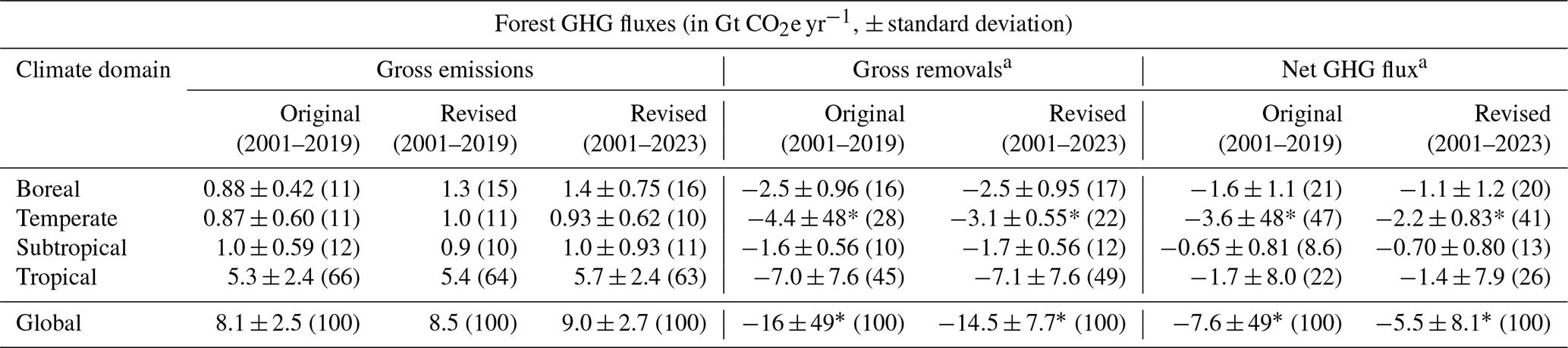
a The revised model does not have gross removals and net flux values for 2001–2019 because they are an annual average over the entire model period, rather than a time series, and thus cannot be calculated for a subset of years.
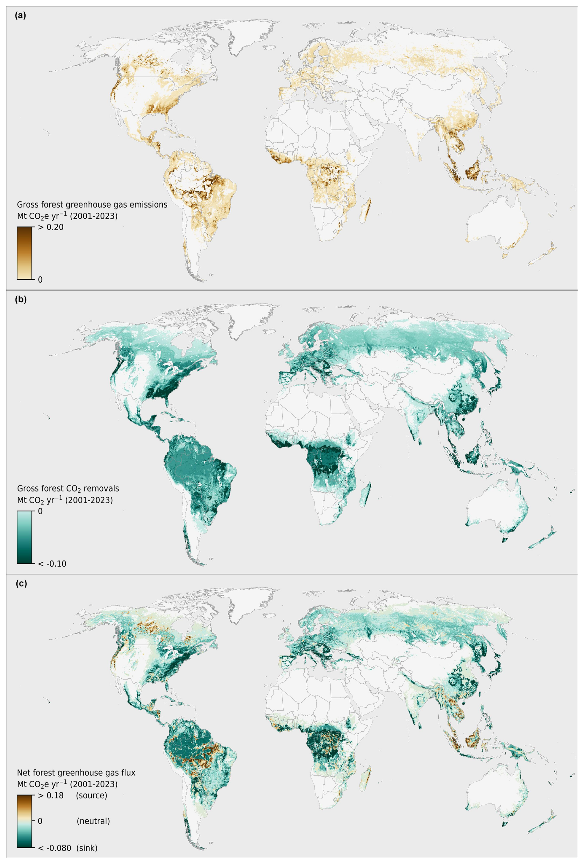
Figure 3Forest-related GHG fluxes (annual average, 2001–2023). (a) Gross GHG emissions. (b) Gross CO2 removals. (c) Net GHG flux. Fluxes are aggregated to 0.04×0.04° (approximately 4×4 km) cells for display purposes. Publisher's remark: please note that the above figure contains disputed territories.
3.2 Effect of GFW model changes on forest carbon flux estimates
Updates to the GFW flux model changed gross emissions, gross removals, and net flux over all spatial scales. Average annual gross emissions in the updated GFW model are 12 % higher than in the original version, primarily due to higher gross annual emissions since 2019 (8.5 Gt CO2e yr−1 between 2001 and 2019 vs. 11.4 Gt CO2e yr−1 between 2020 and 2023). Updated gross annual removals are 7.3% lower than in the original model, primarily due to the use of corrected, lower IPCC Tier 1 removal factors for temperate forests, which are applied to 290 Mha of secondary forests in the framework, primarily throughout Eurasia and Canada. Annual average net GHG flux decreased accordingly by 28 % from the original version because of both higher gross emissions and lower gross removals.
Although we did not quantify the degree to which each change to the model individually affects emissions and removals because we implemented multiple changes simultaneously, we describe how the inputs changed and some general impacts on gross emissions and removals.
For the activity data, we found the following:
-
Temporal coverage of tree cover gain. The area of tree cover gain increased globally from 78 Mha in the original version (gain through 2012) to 130 Mha in the current version (gain through 2020). Carbon removals associated with areas of tree cover gain increased from −0.57 to −0.62 Gt CO2 yr−1. As in the original model, carbon removals occurring in these young (< 20-year-old) forests remain relatively small compared with gross removals occurring in older, established forests that are much more extensive in total area (96 % of gross removals occurred in older forests).
-
Data source for burned area. Use of the new source of fire data with higher spatial resolution (TCLF) combined with an increase in forest fires across Australia, Spain, the USA, and Canada between 2020 and 2023 led to an increase in the global average annual burned area that coincided with tree cover loss from 4.3 Mha yr−1 (2001–2019) to 6.0 Mha yr−1 (2001–2023). Global average emissions increased from 1.0 to 1.7 Gt CO2e yr−1 in areas where tree cover loss was attributed to fire.
-
Data sources for organic soil extent. Improved data led to an increase in the extent of organic soils from 477 to 760 Mha, and the area of tree cover loss on organic soils increased from 0.77 to 2.4 Mha yr−1. Emissions from organic soil drainage in areas with tree cover loss increased from 0.21 to 0.91 Gt CO2e yr−1, occurring primarily in Indonesia and Malaysia (18 % and 3.1 % of the global total, respectively). Higher emissions from organic soil drainage is due to a combination of increased organic soil extent, planted tree extent, and tree cover loss compared with the original model.
-
Data sources for planted tree extent. Planted forest and tree crop extent increased from 140 to 230 Mha, and tree cover loss in planted tree polygons increased from 42 to 64 Mha.
For the emission and removal factors, we found the following:
-
Data source for R : S ratios. The previous global R : S ratio used across the full model extent was 0.26. Now, the average ratio of aboveground removals to belowground removals is 0.27, although with considerable geographic variation.
-
Planted tree removal factors and their uncertainties. The average aboveground removal factor in planted trees was originally 3.2 t C ha−1 yr−1 but it is 2.3 t C ha−1 yr−1 using SDPT v2.0. Global planted forests and trees were originally estimated to be a net sink of −0.30 Gt CO2e yr−1, but they are now a net sink of −0.54 Gt CO2e yr−1 using SDPT v2.0, with the increased area of planted trees compensating for the lower average removal factor.
-
Older (> 20-year-old) secondary temperate forest removal factors and their uncertainties. Older secondary temperate forests using IPCC Tier 1 removal factors (i.e., areas affected by this change) originally covered 310 Mha but now cover 290 Mha. Gross removals in these forests declined from −2.7 to −1.3 Gt CO2 yr−1.
-
Global warming potentials. Updated model results of non-CO2 emissions associated with biomass burning and drainage of organic soils were negligibly impacted by using updated GWPs.
3.3 Updated uncertainty analysis
Nearly all changes to the framework are represented in the error propagation approach and, therefore, affect the global and climate domain uncertainty analyses to some degree. However, the largest change to the uncertainty analysis in terms of input values was the corrected IPCC Tier 1 temperate forest removal factors, which the model applies across large areas of Eurasian and Canadian forests. Some of the largest changes for removal factors and their uncertainties include temperate mountain forest >20 years old (previously 4.4 t AGB ha−1 yr−1 ± 100.7 (± standard deviation), where AGB refers to aboveground biomass; now 2.1 ± 0.02 t AGB ha−1 yr−1) and temperate oceanic forest >20 years old (previously 9.1 t AGB ha−1 yr−1 ± 20.2; now 4.9 ± 0.25 t AGB ha−1 yr−1). We did not formally assess the contributions of individual model changes to uncertainty because the change in IPCC Tier 1 temperate forest removal factor uncertainties was so dominant.
Uncertainty (reported as ± 1 standard deviation) in temperate gross removals declined from 48 Gt CO2 yr−1 in the original GFW model to 0.55 Gt CO2 yr−1, with uncertainty for gross emissions in temperate forests increasing slightly from 0.60 to 0.62 Gt CO2e yr−1 and uncertainty for net flux decreasing from 48 to 0.83 Gt CO2e yr−1 (Table 4). Reduced uncertainty in temperate forest gross removals propagated to reduced uncertainty in global gross removals and net flux. In the uncertainty analysis for the current version of the model, tropical gross removals have the highest uncertainty, driven by relatively high uncertainty in IPCC's Tier 1 removal factors, which the GFW model applies to tropical primary forests and older secondary forests. Large uncertainties for climate domain and global net flux estimates should be interpreted with caution; their uncertainties are proportionately very large, in part because net fluxes reflect the sum of negative (removals) and positive (emissions) terms, compounding the addition of their uncertainties.
3.4 Anthropogenic fluxes from managed forests
When gross CO2 emissions and removals from the GFW flux model for 2001–2022 were reclassified into NGHGI reporting categories, the anthropogenic net flux in managed forest land ranged between −6.9 and −8.6 Gt CO2 yr−1 (with and without emissions from shifting agriculture in secondary forests, respectively) and emissions from deforestation ranged between 3.3 and 5.0 Gt CO2 yr−1 (without and with emissions from shifting agriculture in secondary forests, respectively) (Fig. 4; Table A1 in the Appendix). The resulting net anthropogenic forest flux – the combined flux from both anthropogenic forest land and deforestation – was −3.6 Gt CO2 yr−1. The non-anthropogenic net sink was −2.2 Gt CO2 yr−1, comprised of −2.5 Gt CO2 yr−1 removals and 0.32 Gt CO2 yr−1 emissions from fires and tree cover loss without an assigned driver in unmanaged forests. The combined NGHGI-translated anthropogenic and non-anthropogenic forest sink is about 0.3 Gt CO2 yr−1 larger than the untranslated net flux (−5.8 vs. −5.5 Gt CO2e yr−1, respectively), as the former does not include CH4 and N2O emissions, fluxes from 2023, or fluxes from 32 countries (mostly small island countries) that do not have comparable NGHGIs.
Under the scenario that included emissions from shifting agriculture from secondary forests in deforestation (hatched bars in Fig. 4), GFW's maximum estimate for global deforestation emissions aligned with the combined NGHGI deforestation and organic soil emissions (5.0 Gt CO2 yr−1). In that scenario, GFW's corresponding maximum estimate for the global net sink in anthropogenic forest land was larger than that estimated by NGHGIs. Under the alternative scenario, which included emissions from shifting agriculture in secondary forests in the anthropogenic forest land flux (non-hatched bars in Fig. 4), GFW's minimum estimate for the global net sink in anthropogenic forest land was similar to the NGHGI net forest sink (−6.6 Gt CO2 yr−1), but GFW's corresponding minimum estimate for global deforestation emissions was lower than that estimated by NGHGIs. The combined GFW flux model net anthropogenic forest sink in managed lands is 2.0 Gt CO2 yr−1 greater than in NGHGIs (−1.5 Gt CO2 yr−1).
For Non-Annex 1 countries, the GFW model high and low estimates for forest land and deforestation bracketed the corresponding NGHGI fluxes. However, GFW estimated the net anthropogenic forest flux for Non-Annex 1 countries to be a small net anthropogenic sink, whereas NGHGIs estimated them to be a small net anthropogenic source. For Annex 1 countries, deforestation emissions from the GFW model were much lower than those from NGHGIs (0.046–0.049 and 0.55 Gt CO2 yr−1, respectively) and the net forest sink was somewhat larger (−3.2 and −2.3 Gt CO2 yr−1, respectively).
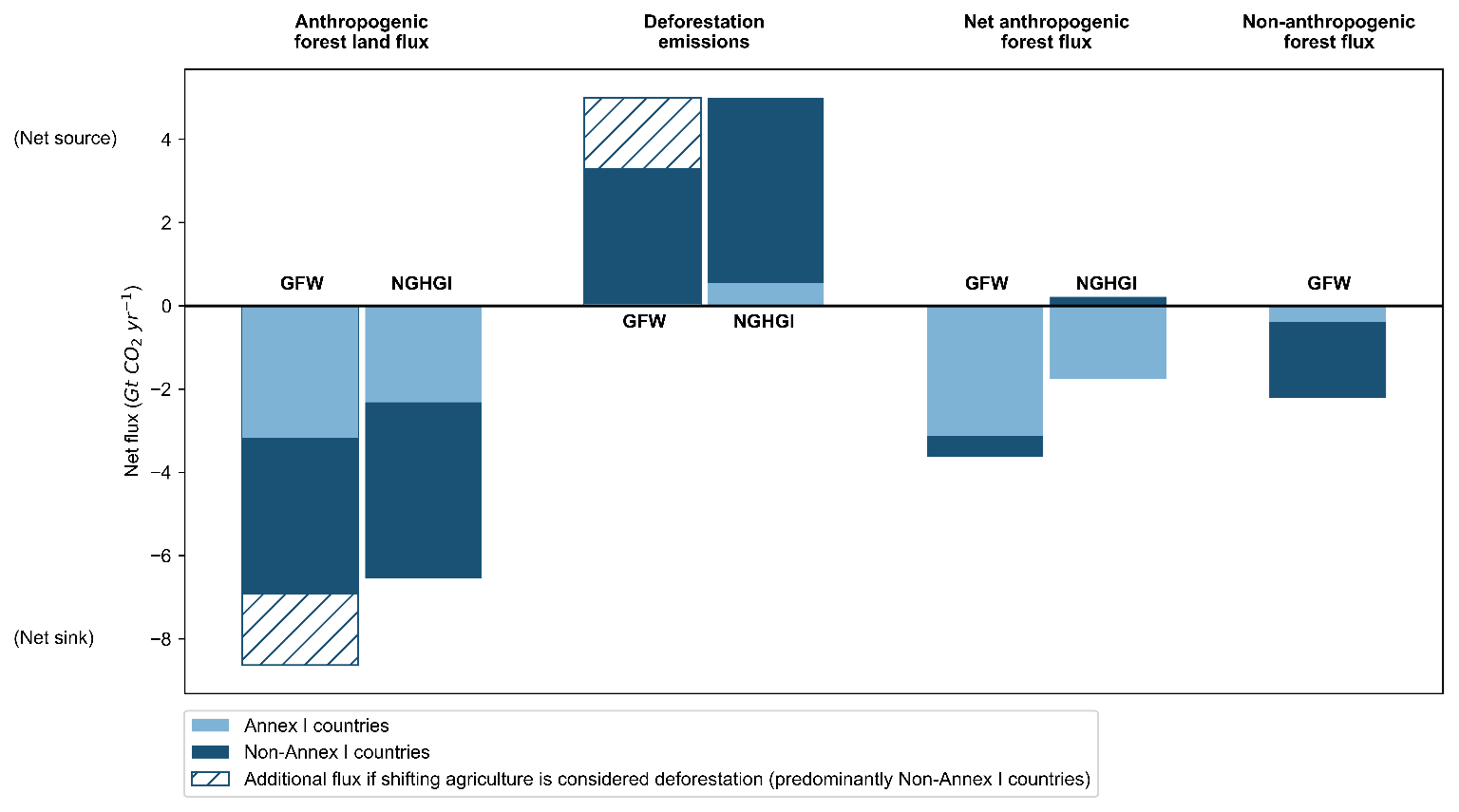
Figure 4Comparison of average annual forest carbon fluxes (2001–2022) between national greenhouse gas inventories (NGHGIs) and the updated GFW flux model. For the GFW flux model, net anthropogenic forest flux is calculated as the sum of the net anthropogenic forest land flux in managed forests and deforestation (Sect. 2.3). Non-anthropogenic forest flux is calculated as emissions and removals occurring outside of managed forests. Because country reporting on emissions from the loss of secondary forests associated with cycles of shifting agriculture is ambiguous, these emissions are shown as hatched bars for the GFW model to indicate how they impact totals depending on the reporting category (forest land or deforestation). Results from the GFW model are for CO2 fluxes only, and NGHGI results have also been limited to CO2 fluxes except for a few developing countries where non-CO2 emissions could not be separated.
Although the magnitude of the global GFW model estimates for deforestation emissions and the anthropogenic sink in forests align with the aggregated NGHGIs for 2001–2022 under different scenarios, their trends from 2001 to 2022 do not agree (Fig. 5). Both globally and for Non-Annex 1 countries, the NGHGIs suggest that forest land became a slightly larger sink from 2001 to 2022 and that deforestation emissions lacked a clear trend during the aforementioned period. However, the GFW flux model results suggest the opposite: a reduced sink in forest land and increased deforestation emissions. The forest land flux and deforestation emissions from NGHGIs and the GFW model for Non-Annex 1 countries appear to converge in the last 10 years (roughly −6 Gt CO2 yr−1 and 5 Gt CO2 yr−1, respectively). For Annex 1 countries, the forest land sink decreased much more according to the GFW model than NGHGIs, while deforestation emissions stayed fairly constant in both.
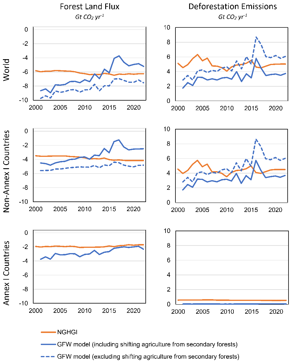
Figure 5Comparison of forest carbon flux time series (2001–2022) between the national greenhouse gas inventories (NGHGIs) and the updated GFW flux model for the world, Non-Annex 1 countries, and Annex 1 countries. The NGHGI values shown here exclude any fluxes from harvested wood products, and deforestation emissions are the combined emissions from both deforestation and organic soils to conceptually align with the scope of fluxes from the GFW framework. For the world and Non-Annex 1 countries, the GFW model results are shown in two time series: one in which emissions from shifting agriculture in secondary forests are included in that reporting category and one in which those emissions are not included. For the GFW model in Annex 1 countries, the two scenarios are essentially the same; thus, we show only one line. The GFW model has been limited to CO2 only; NGHGI data include only CO2 except for a few developing countries where non-CO2 emissions could not be separated.
We focus our discussion on the following topics. First, we examine how the updated GFW forest flux model compares with results from a recent global estimate of forest fluxes by Pan et al. (2024) and the Global Carbon Budget (GCB). Second, we discuss how fully geospatial, Earth-observation-based forest flux estimates can be translated into the reporting categories of NGHGIs and how transparency in both approaches can result in methodological improvements. Third, we discuss strengths and limitations of GFW's Earth-observation-based forest carbon flux model. Fourth, we outline future research priorities which provide partial solutions to the model's current limitations.
4.1 Comparison with other recent global flux estimates
Pan et al. (2024) is a relevant comparison for the GFW model, as both include only forests and report gross rather than net fluxes. Pan et al. (2024) estimated gross removals by forests, gross emissions from tropical deforestation, and the global forest carbon sink by synthesizing forest plot data (inventories and long-term monitoring sites) from 1990 onwards. The removal estimates are conceptually similar (e.g., both include established and new forests), but the emission estimates have a different geographic scope (global for GFW but tropical for Pan et al., 2024) (Table 5). The global net fluxes from Pan et al. (2024) and the updated GFW model are remarkably similar given their entirely different approaches, and thus provide multiple lines of evidence for a net forest sink of approximately −6 Gt CO2 yr−1. Differences in gross emissions and removals between the data sources likely arise from different scopes and system boundaries, but they may be balanced out when combined in the global net flux. Pan et al. (2024) estimated higher tropical gross emissions than the GFW model did for the tropics and subtropics for 2001–2019. When the GFW model's gross emissions (CO2 only) are limited to the tropics and subtropics and one geospatially implemented definition of deforestation (tree cover loss due to shifting agriculture in primary forest as well as all commodity- and urbanization-driven tree cover loss), it estimates 3.2 Gt CO2 yr−1, well below the tropical deforestation estimate of Pan et al. (2024). When more broadly including all tree cover loss in the tropics and subtropics, the GFW model estimates gross emissions of 6.3 Gt CO2 yr−1.
Table 5Comparison of GFW flux model results to Pan et al. (2024) and the Global Carbon Budget (GCB). Estimates from the three data sources are not directly comparable due to differences in scope, data, methodologies, and reporting structure. GFW model fluxes are limited to 2001–2022 for comparability with the GCB. The GFW model and Pan et al. (2024) are for forests only, while the GCB also includes non-forest land.
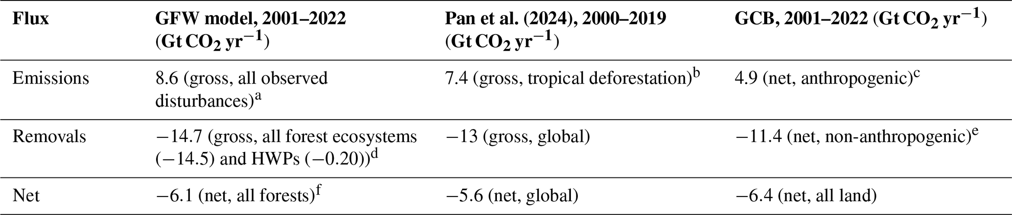
a Gross emissions from all forest disturbances (anthropogenic and non-anthropogenic) for 2001–2022. Estimate includes CO2 only for comparability with the GCB; non-CO2 emissions are 0.19 Gt CO2e yr−1. This value is lower than that in Table 4 (9.0 Gt CO2e yr−1), as this one includes emissions for 2001–2022 only and excludes non-CO2 gases. b Includes emissions from degradation. c Estimates only net direct anthropogenic effects, including deforestation, afforestation/reforestation, organic soils, and wood harvest. Gross fluxes higher but not reported. d Gross removals from all forest processes (direct, indirect, and natural). HWPs are transfers to harvested wood products. Removals are the annual average from 2001 to 2023. e Represents the land sink associated with indirect human-induced effects such as CO2 fertilization and nitrogen deposition. f Calculated as the net balance between gross forest ecosystem emissions and removals (8.6–14.5 Gt CO2 yr−1) in this table plus an additional net removal of −0.20 Gt CO2 yr−1 into HWPs. This value differs from that in Table 4 (−5.5 Gt CO2e yr−1), as this one uses lower gross emissions (see note a).
Another point of comparison is the GCB, released by the Global Carbon Project each year. The GCB provides annual estimates of GHG emissions and carbon sinks, when relevant, for all sectors. The GFW flux model is not designed to represent the land portion of the global carbon cycle, nor is it directly comparable with the land use fluxes included in the GCB because of differences in definitions, scope, reporting structure, and methods (Friedlingstein et al., 2023). Three overarching differences are as follows: (1) the GCB reports net sources and sinks for all land (including croplands, grasslands, semi-arid savannas, and shrublands), while the GFW model reports gross emissions and removals for forests only; (2) the GCB categorizes fluxes by process into net anthropogenic emissions from land use change and forestry and the “natural” land sink, while the GFW model categorizes fluxes by activity data; (3) the GCB uses global bookkeeping models to estimate net anthropogenic carbon fluxes from land use and dynamic global vegetation models (DGVMs) to estimate net carbon fluxes from the natural land sink (Walker et al., 2024), while the GFW flux model uses a single integrated approach to estimate emissions and removals. Nevertheless, comparison of the GFW model with the GCB is useful because they use entirely different data sources and approaches, and, as such, convergence between them would represent multiple lines of evidence towards the magnitude of the land sink.
We estimated a global net CO2 sink by forest ecosystems of −6.1 Gt CO2 yr−1 between 2001 and 2022, which is similar to the net CO2 land sink of −6.4 Gt CO2 yr−1 in the GCB for all terrestrial fluxes over the same period (Table 5). The GCB's net emission estimate (4.9 Gt CO2 yr−1) is lower than GFW's gross emissions estimate (8.6 Gt CO2 yr−1), partially because the GCB's land use change emissions (sources) reflect the net balance between anthropogenic emissions and anthropogenic removals associated with forest regrowth. Similarly, the GFW model's gross removals reflect removals across all forest lands, including removals implicit (but unreported) in the GCB net land use change estimate (Friedlingstein et al., 2023). Additional reclassification of fluxes from the GFW model into net anthropogenic fluxes from land use change and the natural land sink may be possible for further comparisons with the GCB, as has been done between the GCB and NGHGIs (Schwingshackl et al., 2022).
In the comparison of the original GFW model with the GCB, we included a nonspatial estimate of emissions from tropical forest degradation of 2.1 Gt CO2e yr−1 from Pearson et al. (2017) that potentially included some emissions from small-scale disturbances which we assumed our original model did not capture. For this and subsequent comparisons between the GFW flux framework and the GCB, we are discontinuing the inclusion of a nonspatial estimate of degradation emissions from a source external to our framework to maintain its internal consistency and fully geospatial nature. We acknowledge that the GFW model itself is likely omitting both emissions (e.g., from degradation not detected by TCL) and removals (e.g., from low canopy density or regenerating forest), but those are gaps that the model should be able to fill over time (see Sect. 4.4). Adding external data such as Pearson et al. (2017) results in the risk of double-counting emissions in the global total. As more geospatial data on distinguishing deforestation from degradation (Vancutsem et al., 2021) become available globally and geospatial data on the emission and removal factors associated with forest degradation (Holcomb et al., 2024) and recovery (Heinrich et al., 2023b) are developed, it may be possible to reintegrate forest degradation and its associated fluxes.
4.2 Translating between Earth-observation-based fluxes and NGHGIs
The 6.7 Gt CO2 yr−1 gap in global land use emissions between NGHGIs and the GCB has been largely explained (Grassi et al., 2023), and translation between NGHGIs (on the one hand) and bookkeeping models and DGVMs (on the other hand) is becoming routine (e.g., Schwingshackl et al., 2022); this work is the start of a similar process for explaining the gap between NGHGIs and Earth-observation-based models, primarily via the reallocation of emissions and removals to match NGHGIs' land use categories and filtering the results with maps of managed forest as a proxy to delineate anthropogenic from non-anthropogenic fluxes. This approach follows the recommendations of the recent IPCC Expert Meeting on Reconciling Land Use Emissions (IPCC, 2024). Our goal in translating GFW model results into a NGHGI reporting framework was to provide independent estimates of forest-based GHG fluxes based on globally consistent Earth-observation-based data in the reporting categories that national policymakers use. It was not to reproduce how countries classify their managed land, report their forest fluxes in practice, or compare fluxes for individual countries. For example, we did not rely solely on the use of managed land polygons for Case 2a countries to define managed forest; if our observations detected direct human activity in unmanaged polygons, we assigned those fluxes to anthropogenic forest land fluxes or deforestation. Thus, although this translation makes the GFW model more conceptually similar with NGHGIs in that the outputs are supposed to represent the same fluxes, they are still not necessarily entirely comparable because we did not exactly reproduce what countries do in practice within their NGHGIs. This demonstrates that the GFW model is sufficiently flexible to approximate the system boundaries of anthropogenic fluxes in the IPCC reporting framework and that Earth-observation-based models can be used to independently monitor anthropogenic GHG fluxes from forests if adequate country data are made publicly available.
Although the conceptual alignment produces quantitatively similar annual average fluxes for the GFW model and NGHGIs globally and for Non-Annex 1 countries, the trends from NGHGIs and the GFW model differ (Fig. 5). For Non-Annex 1 countries, where the trends in each data source are most evident, NGHGIs reported the forest land sink strengthening slightly, while deforestation emissions fluctuated but were generally steady. The GFW model, on the other hand, reported a weakening sink in forest land and deforestation emissions that increased correspondingly. The decreasing forest land sink in the GFW model is due to the use of average annual gross removals over time (i.e., a constant value), combined with increasing (i.e., annually variable) tree cover losses not associated with deforestation. In NGHGIs, forest land and deforestation can both change through time. The differing trends between the GFW flux model and aggregated NGHGIs is likely driven by generally increasing annual tree cover loss used in GFW (Hansen et al., 2013), as that has the greatest interannual variability present in either dataset. Quantitative similarity between the GFW model and NGHGIs may be further improved when the GFW model's gross removals can vary through time as well (Sect. 4.4). Moreover, for Non-Annex 1 countries, results from the GFW model and NGHGIs have converged for forest land and deforestation since around 2010, with the two GFW model scenarios bracketing NGHGI fluxes from both reporting categories after that year. This indicates that the GFW model and the tree cover loss data that underlie its gross emissions were perhaps under-detecting loss relative to NGHGIs in the early part of the time series.
Exploration of the differences between the GFW model and specific countries' NGHGIs is beyond the scope of this paper; future work may include more detailed reclassification of the GFW model's fluxes and comparisons with specific regions or countries. As an initial resource for country-level data, the European Union Joint Research Centre LULUCF data hub presents graphs of national land fluxes according to their NGHGIs, the Global Carbon Budget, and the translated fluxes from the GFW model (https://forest-observatory.ec.europa.eu/carbon/fluxes, last access: 11 March 2025). Further sub-setting results from our framework to differentiate anthropogenic and non-anthropogenic fluxes for comparison with NGHGIs for individual regions, countries, and other local-scale analyses is possible and encouraged. Indeed, comparison of the GFW model and countries' inventories is a way to explore the complementarity and discrepancies between Earth observation data and inventories, encourage transparency for both, and improve both approaches (Heinrich et al., 2023a). For example, one advantage of the GFW model, which includes forest fluxes undifferentiated by human contribution, is that it encompasses both anthropogenic and non-anthropogenic fluxes. When this translation exercise is conducted, GHG fluxes from managed forests can be put in the context of all forest fluxes and compared with fluxes from unmanaged forests. Because NGHGIs are not required to estimate fluxes from unmanaged land (just to report the area of unmanaged land), aggregation of NGHGIs does not provide context for managed land fluxes with unmanaged land fluxes. In other words, the GFW model can indicate the scale of non-anthropogenic fluxes that countries are not reporting in their NGHGIs (which nevertheless affect atmospheric CO2 concentrations and global temperature), while NGHGIs are necessary for the GFW model to approximate the anthropogenic fluxes that are being monitored by countries and the focus of the Paris Agreement. An alternative approach for reconciling global models and NGHGIs would be for NGHGIs to report all land fluxes in the country, in both managed and unmanaged land (Nabuurs et al., 2023), but adoption of this seems unlikely.
While our geospatial, Earth-observation-based framework permits estimation of fluxes for any geospatially defined forest and the inclusion (or exclusion) of any area of interest, it cannot distinguish between managed vs. unmanaged land without relevant spatial data. Thus, the ability of the GFW model, and Earth observation models in general, to be translated into IPCC categories largely depends on the transparency with which countries report on their managed lands. Only three countries have publicly available maps of managed and unmanaged forest (Canada, Brazil, and the USA) (Ogle et al., 2018). For all remaining countries, the use and application of the managed land proxy were assumed based on the available information from country reports. In the absence of this information, maps of primary or intact forest have been used as a proxy for unmanaged forest. With sufficient transparency and flexibility in both the Earth-observation-based products and NGHGIs, the differences between them can be explored.
A key driver of forest disturbance, and thus emissions, in the GFW model is shifting agriculture. However, the comparison between GFW and NGHGIs is complicated by the fact that countries typically do not provide specific information on shifting agriculture in their land representation; according to the IPCC guidelines, it can be implicitly included either in forest or in other land uses (e.g., cropland) (Grassi et al., 2023). Thus, we developed two scenarios for the treatment of fluxes from shifting agriculture (Fig. 4). Hopefully, as countries begin to submit their biennial transparency reports under the Paris Agreement, their use of the managed land proxy, the treatment of shifting agriculture, and other exclusions from inventories will be progressively clarified, and translation between approaches will become more accurate. Although they are time-consuming to implement, the goal should be for the kinds of Earth-observation-based adjustments described by Heinrich et al. (2023a) for Brazil to be achievable for all countries. This will ultimately facilitate comparisons between global models such as the GFW model and NGHGIs, provide national policymakers with timely geospatial data in their own reporting terms, and build confidence in the magnitude and trends of land-based anthropogenic emissions and sinks (Grassi et al., 2023).
Future improvements to our flux reclassifications, which may improve regional or country-level comparisons, could include customizing tree cover density thresholds that align more closely with countries' forest definitions to filter forest extent and, thus, the associated fluxes on a country-by-country basis. Additionally, we used maps of primary forests and intact forest landscapes from 2001 and 2000, respectively, to approximate the extent of unmanaged forests at the initial year of our model framework. Further refinement to the GFW model's estimates of fluxes from managed lands could include recategorizing forests as managed or unmanaged using updated primary/intact forest boundaries in different years to reflect changes to countries' managed land area over time whenever known. Furthermore, for simplicity, we considered all forest removals as forest land and did not differentiate the relatively small amount of removals from forest gain as “other land converted to forest”, which is a category that countries report in their NGHGIs. Another improvement would be to separate the emissions from drainage of organic soils and the emissions from deforestation in the GFW model; in the current translation, deforestation emissions and organic soil emissions are combined in both data sources. Separating them would refine the conceptual similarity. This would matter most in countries with high emissions from organic soils. Finally, emissions from fires occurring in unmanaged land could theoretically be differentiated into anthropogenic vs. non-anthropogenic using additional geospatial data, rather than our simplified assumption that all fires in unmanaged forests are of non-anthropogenic origin.
4.3 Strengths and limitations of the GFW flux monitoring framework
The strengths of the current GFW flux model are broadly similar to those described in Harris et al. (2021). Strengths include its transparency, operational nature, flexibility, and updatability as new information becomes available. Here, we focus on the complementarity of the GFW model with other land flux monitoring approaches. A strength of flux monitoring based on Earth observation (and therefore geospatial) data is its geographic specificity, while maintaining spatial consistency. Knowing where changes in land use and land cover – and the emissions and removals they have caused – occurred may help identify what factors are responsible for these changes and how to attribute them to specific human activities. While detailed information from ground surveys and activity data generated using local training data may provide more detail and accuracy at local scales, understanding the magnitude and distribution of global change requires a combination of both ground- and space-based observations (Houghton and Castanho, 2023). In this sense, it fills in the gaps among other flux monitoring approaches. In terms of global consistency, the GFW model's key data are global in breadth and independent of data from the United Nations Food and Agriculture Organization, giving it a separate source for forest change data from bookkeeping models (Hansis et al., 2015; Gasser et al., 2020; Houghton and Castanho, 2023). Moreover, by having an open-source model based on publicly available data, others can evaluate the model, make improvements, and/or adapt it to use national or local (rather than global) data. Users can keep some defaults while replacing others with better or more specific information and can understand how results are impacted by the various changes made for regions or at scales that interest them most.
Limitations are also broadly similar to those described in Harris et al. (2021). First, combining multiple spatially explicit data sources compounds the errors present in each individual source used in the framework. The GFW model partially manages this over larger areas through uncertainty propagation analysis to identify the relative contributions of different model components to uncertainty in each climate domain, but it cannot provide a pixel-level accuracy or uncertainty map. Extending the uncertainty framework to smaller regions (e.g., biomes or countries) would require uncertainty information for each of the individual data sources to be available at the desired scale of uncertainty propagation analysis. Second, the gain–loss approach of starting with baseline carbon densities and adding gains and subtracting losses over time has the potential to generate unrealistic estimates over longer periods due to drift from the original benchmark map. The GFW model could potentially address this through recalibration of carbon densities and forest extent at one or more intermediate years (e.g., 2010 and 2015). Finally, the GFW model continues to have temporal limitations for both activity data and removal factors. The shorter gain period compared with tree cover loss in the original publication (12 vs. 19 years, respectively) has largely been addressed with the extension of tree cover gain through 2020. More limiting than the mismatch of tree cover loss and gain durations is the non-temporal nature of the tree cover gain map. Because the year of tree cover gain is not known, the model does not necessarily include post-disturbance gross regrowth and removals, which may underestimate removals and decrease the net sink. This effect would be particularly pronounced in forest where disturbance occurs earlier in the model and regrowth is substantial. The tree cover loss time series also has its own inconsistencies (Weisse and Potapov, 2021). The improvement in Earth observation data and changes to processing confound apparent trends in gross emissions based on tree cover loss; it is difficult to determine how much the trends in emissions are due to real increases vs. better detection of disturbances through time. For removal factors, the concern is not so much temporal inconsistency as temporal constancy; the model makes the simplifying assumption of static removal factors (i.e., removal factors do not change as forests grow or climate changes over the 23-year model period). Thus, the GFW model does not incorporate growth–response curves or climate feedbacks, unlike in Earth system models.
4.3.1 Research priorities and anticipated model developments
Beyond annual updates to the GFW model, we anticipate continued, substantial changes to and research around both activity data and emission and removal factors. These do not change the underlying conceptual framework but rather its implementation as the model.
For activity data, anticipated model developments include the following:
-
Global forest change data. The model will use annual forest extent, loss, and gain maps for greater temporal detail (similar to Potapov et al., 2019, or Turubanova et al., 2023) and improved representation of carbon dynamics. For example, the year of tree cover gain will be known (at least approximately) and repeated forest disturbances in the same location will be captured (unlike in Hansen et al., 2013), allowing the generation of annual time series of gross emissions, gross removals, and net flux. This should further enhance comparability of temporal trends in GFW's fluxes with the GCB and NGHGIs.
-
Drivers of forest loss. The model currently uses a global map of drivers of forest loss at a 10 km resolution (Curtis et al., 2018, updated to 2023), but research on mapping drivers of forest loss is advancing. An anticipated 1 km resolution global map of drivers of forest loss (Sims et al., 2025) will detect drivers that are not dominant at 10 km (and are therefore not mapped) but are important at smaller scales, such as loss due to small-scale infrastructure and built-up areas amid loss due to agricultural commodity expansion. Moreover, a separate class of forest loss due to natural disturbances will further help with parsing natural and anthropogenic fluxes for translation into NGHGI reporting categories.
-
Delineation of organic soils and their drainage status. The GFW model currently compiles several different data sources (Table 2), which have different definitions and resolutions, to map organic soil extent. The GFW model would benefit from a globally consistent organic soil map based on a comprehensive aggregation of soil samples and standardized mapping methods. However, it is not just the extent of organic soils but their drainage that affects emissions in the GFW model. Thus, we are exploring improved mapping of organic soil drainage using recent improvements in delineating road networks (OSM, 2010; Meijer et al., 2018; Engert et al., 2024), drainage canal networks (Dadap et al., 2021), and land cover (Potapov et al., 2022a). More comprehensive maps of organic soil extent and drainage will improve where the GFW model reports these emissions, particularly affecting non-CO2 GHG emissions.
-
Improved initial forest age map. The GFW model currently classifies forested pixels into primary forest, secondary forest > 20 years old, and secondary forest < 20 years old in 2000 using a few simple rules (described in Harris et al., 2021). However, a forest age map such as Besnard et al. (2021) could be used to refine the assignment of starting age categories – particularly for secondary forests – or to determine where forest is along age–growth curves.
-
Extent of planted forests and trees. The model currently uses SDPT v2.0 (Richter et al., 2024), but plans are underway for SDPT v3.0, which will improve differentiation between natural and artificial stands in the USA and Canada, along with other improvements for delineating planted tree extent in other countries.
For emission and removal factors, anticipated model developments include the following:
-
Improved spatial and temporal resolution of forest carbon removals. The dominant role of removal factor uncertainties in the uncertainty analysis highlights the need to further improve understanding of spatial and temporal variation in forest carbon removals. Combining plot-level biomass estimates with spaceborne observations to produce static biomass maps is well established (e.g., Saatchi et al., 2011; Santoro et al., 2021) and mapping biomass change is being explored (Xu et al., 2021), but these methods do not provide spatiotemporally variable removal factors. An ecology-based, yet still spatial, way to map removal factors could combine tree-level information collected in field plots with machine learning methods to map forest population structure through time, including variables that influence biomass change like upgrowth, mortality, and recruitment for different forest types (Ma et al., 2020). Such an approach can generate spatial and temporal predictions of how biomass changes across space and time that can be validated with forest plot data. In conjunction with a time series of tree cover gain (in activity data list above), this would result in fully temporal gross removals. Alternatively, growth curves for natural regeneration of forests could be revised and expanded to include a greater range of forest ages, using similar methods to Cook-Patton et al. (2020) (Robinson et al., 2025).
-
Improved maps of soil carbon dynamics in mineral soils. The GFW model currently uses a benchmark map of soil organic carbon (SOC) density in mineral soil in 2000 and assumes loss of specific fractions of carbon under certain types of tree cover loss, following a Tier 1 approach from IPCC 2019. However, a time series of soil organic carbon density in mineral soil would support more realistic mapping of SOC losses and gains.
-
Improved maps of emissions from organic soil drainage. The GFW model currently assumes that organic soils are drained only wherever tree cover loss, organic soils, and planted trees (Richter et al., 2024) coincide. Future improvements could include (1) expanding the proxies used to map organic soil drainage and (2) incorporating emissions from the extraction of organic soils.
Additionally, opportunities remain to compare GFW model emissions and removals with NGHGIs, bookkeeping models, and regional or local data (e.g., Araza et al., 2023; Heinrich et al., 2023b). Such work would further our understanding of the complementary roles of Earth-observation-based forest carbon models and other approaches to forest flux monitoring.
Gross emissions, gross removals, and net flux are available for download as 10 × 10° GeoTIFFs at 0.00025 × 0.00025° resolution. Data that correspond to the model version presented in this publication are as follows: gross removals (Gibbs et al., 2024a) – https://doi.org/10.7910/DVN/V2ISRH; gross emissions (Gibbs et al., 2024b) – https://doi.org/10.7910/DVN/LNPSGP; and net flux (Gibbs et al., 2024c) – https://doi.org/10.7910/DVN/TVZVBI. Data are also available as assets on Google Earth Engine at https://code.earthengine.google.com/ae55707e335894d7be515386195390d2 (last access: 10 January 2025). Note that more recent versions of these datasets may be available from https://www.globalforestwatch.org (last access: 11 March 2025). The code is available from https://github.com/wri/carbon-budget (Gibbs et al., 2024d).
The updated Earth-observation-based GFW forest carbon flux framework continues to show a substantial net sink for CO2 in forests globally, while also reporting gross emissions over half as large as gross removals since 2001. This highlights ongoing opportunities to protect the forest carbon sink across a broad area and also reduce emissions from forest loss, especially in hotspots of emissions that are discernable with our geospatial framework. The revised uncertainty analysis – with its dramatic reduction in uncertainty in gross removals – demonstrates the importance of refining forest carbon sequestration rate estimates. The flexibility of the model supports analyses at a range of spatial scales, while its operational nature means it can incorporate new and existing Earth observation products and provide timely maps and data. Our translation of the GFW model's fluxes into the reporting framework that NGHGIs use – following the recommendations of the recent IPCC Expert Meeting on Reconciling Land Use Emissions (IPCC, 2024) – provides another lens through which to look at country-level, land-based climate mitigation and is a resource for national policymakers interested in timely spatial data on land fluxes. It also demonstrates the two approaches' ability to improve, assess, and potentially confirm each other. Ultimately, confidence and transparency are needed in assessments of progress towards the Paris Agreement, and Earth-observation-based forest carbon models are another tool to build consensus.
Table A1Comparison of forest carbon fluxes in Annex 1 countries, Non-Annex 1 countries, and globally between the GFW flux model and national greenhouse gas inventories (NGHGIs). Here, ranges in reported GFW values come from two different scenarios: one scenario in which emissions from shifting agriculture in secondary forests are included in forest land and one scenario in which all emissions from shifting agriculture in deforestation are included. Results from the GFW model are for CO2 fluxes only, and NGHGI results have also been limited to CO2 fluxes except for a few developing countries where non-CO2 emissions could not be separated.
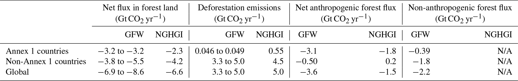
NH and DAG conceived the model updates, and DAG and MR executed the model updates. DAG executed the updated uncertainty analysis. GG, SR, and JM created the national greenhouse gas inventory dataset, and MR and GG compared it to the GFW model. VH contributed to the translation of the GFW model for Brazil. DAG led manuscript preparation with contributions from all co-authors.
The contact author has declared that none of the authors has any competing interests.
Publisher's note: Copernicus Publications remains neutral with regard to jurisdictional claims made in the text, published maps, institutional affiliations, or any other geographical representation in this paper. While Copernicus Publications makes every effort to include appropriate place names, the final responsibility lies with the authors.
This work received support from Norway's International Climate and Forest Initiative (grant number 18/2721) and the Bezos Earth Fund (grant number 2022-00805).
This paper was edited by Nophea Sasaki and reviewed by two anonymous referees.
Araza, A., Herold, M., de Bruin, S., Ciais, P., Gibbs, D. A., Harris, N., Santoro, M., Wigneron, J.-P., Yang, H., Málaga, N., Nesha, K., Rodriguez-Veiga, P., Brovkina, O., Brown, H. C. A., Chanev, M., Dimitrov, Z., Filchev, L., Fridman, J., García, M., Gikov, A., Govaere, L., Dimitrov, P., Moradi, F., Muelbert, A. E., Novotný, J., Pugh, T. A. M., Schelhaas, M.-J., Schepaschenko, D., Stereńczak, K., and Hein, L.: Past decade above-ground biomass change comparisons from four multi-temporal global maps, International Journal of Applied Earth Observation and Geoinformation, 118, 103274, https://doi.org/10.1016/j.jag.2023.103274, 2023.
Austin, K. G., Mosnier, A., Pirker, J., McCallum, I., Fritz, S., and Kasibhatla, P. S.: Shifting patterns of oil palm driven deforestation in Indonesia and implications for zero-deforestation commitments, Land Use Policy, 69, 41–48, https://doi.org/10.1016/j.landusepol.2017.08.036, 2017.
Besnard, S., Koirala, S., Santoro, M., Weber, U., Nelson, J., Gütter, J., Herault, B., Kassi, J., N'Guessan, A., Neigh, C., Poulter, B., Zhang, T., and Carvalhais, N.: Mapping global forest age from forest inventories, biomass and climate data, Earth Syst. Sci. Data, 13, 4881–4896, https://doi.org/10.5194/essd-13-4881-2021, 2021.
Brus, D. J., Hengeveld, G. M., Walvoort, D. J. J., Goedhart, P. W., Heidema, A. H., Nabuurs, G. J., and Gunia, K.: Statistical mapping of tree species over Europe, Eur. J. Forest Res., 131, 145–157, https://doi.org/10.1007/s10342-011-0513-5, 2012.
Cook-Patton, S. C., Leavitt, S. M., Gibbs, D., Harris, N. L., Lister, K., Anderson-Teixeira, K. J., Briggs, R. D., Chazdon, R. L., Crowther, T. W., Ellis, P. W., Griscom, H. P., Herrmann, V., Holl, K. D., Houghton, R. A., Larrosa, C., Lomax, G., Lucas, R., Madsen, P., Malhi, Y., Paquette, A., Parker, J. D., Paul, K., Routh, D., Roxburgh, S., Saatchi, S., van den Hoogen, J., Walker, W. S., Wheeler, C. E., Wood, S. A., Xu, L., and Griscom, B. W.: Mapping carbon accumulation potential from global natural forest regrowth, Nature, 585, 545–550, https://doi.org/10.1038/s41586-020-2686-x, 2020.
Crezee, B., Dargie, G. C., Ewango, C. E. N., Mitchard, E. T. A., Emba B., O., Kanyama T., J., Bola, P., Ndjango, J.-B. N., Girkin, N. T., Bocko, Y. E., Ifo, S. A., Hubau, W., Seidensticker, D., Batumike, R., Imani, G., Cuní-Sanchez, A., Kiahtipes, C. A., Lebamba, J., Wotzka, H.-P., Bean, H., Baker, T. R., Baird, A. J., Boom, A., Morris, P. J., Page, S. E., Lawson, I. T., and Lewis, S. L.: Mapping peat thickness and carbon stocks of the central Congo Basin using field data, Nat. Geosci., 15, 639–644, https://doi.org/10.1038/s41561-022-00966-7, 2022.
Curtis, P. G., Slay, C. M., Harris, N. L., Tyukavina, A., and Hansen, M. C.: Classifying drivers of global forest loss, Science, 361, 1108–1111, https://doi.org/10.1126/science.aau3445, 2018.
Dadap, N. C., Hoyt, A. M., Cobb, A. R., Oner, D., Kozinski, M., Fua, P. V., Rao, K., Harvey, C. F., and Konings, A. G.: Drainage Canals in Southeast Asian Peatlands Increase Carbon Emissions, AGU Advances, 2, e2020AV000321, https://doi.org/10.1029/2020AV000321, 2021.
Dorgeist, L., Schwingshackl, C., Bultan, S., and Pongratz, J.: A consistent budgeting of terrestrial carbon fluxes, Nat. Commun., 15, 7426, https://doi.org/10.1038/s41467-024-51126-x, 2024.
Engert, J. E., Campbell, M. J., Cinner, J. E., Ishida, Y., Sloan, S., Supriatna, J., Alamgir, M., Cislowski, J., and Laurance, W. F.: Ghost roads and the destruction of Asia-Pacific tropical forests, Nature, 629, 370–375, https://doi.org/10.1038/s41586-024-07303-5, 2024.
European Council: Regulation – 2018/841 – EN – EUR-Lex: https://eur-lex.europa.eu/eli/reg/2018/841/oj (last access: 30 July 2024), 2018.
FAO: Global planted forest thematic study: results and analysis, edited by: Del Lungo, A., Ball, J., and Carle, J., Planted Forests and Trees Working Paper 38, FAO Rome, Italy, https://openknowledge.fao.org/server/api/core/bitstreams/5697e770-6a6b-42b0-90f8-35e1f0e33223/content (last access: 15 January 2025), 2006.
FAO: Global ecological zones for FAO forest reporting, FAO Rome, Italy, 2012.
FAO: FAOSTAT, https://www.fao.org/faostat/en/ (last access: 11 March 2025), 2024.
Farr, T. G., Rosen, P. A., Caro, E., Crippen, R., Duren, R., Hensley, S., Kobrick, M., Paller, M., Rodriguez, E., Roth, L., Seal, D., Shaffer, S., Shimada, J., Umland, J., Werner, M., Oskin, M., Burbank, D., and Alsdorf, D.: The Shuttle Radar Topography Mission, Rev. Geophys., 45, RG2004, https://doi.org/10.1029/2005RG000183, 2007.
Fick, S. E. and Hijmans, R. J.: WorldClim 2: new 1-km spatial resolution climate surfaces for global land areas, Int. J. Climatol., 37, 4302–4315, https://doi.org/10.1002/joc.5086, 2017.
Friedlingstein, P., O'Sullivan, M., Jones, M. W., Andrew, R. M., Bakker, D. C. E., Hauck, J., Landschützer, P., Le Quéré, C., Luijkx, I. T., Peters, G. P., Peters, W., Pongratz, J., Schwingshackl, C., Sitch, S., Canadell, J. G., Ciais, P., Jackson, R. B., Alin, S. R., Anthoni, P., Barbero, L., Bates, N. R., Becker, M., Bellouin, N., Decharme, B., Bopp, L., Brasika, I. B. M., Cadule, P., Chamberlain, M. A., Chandra, N., Chau, T.-T.-T., Chevallier, F., Chini, L. P., Cronin, M., Dou, X., Enyo, K., Evans, W., Falk, S., Feely, R. A., Feng, L., Ford, D. J., Gasser, T., Ghattas, J., Gkritzalis, T., Grassi, G., Gregor, L., Gruber, N., Gürses, Ö., Harris, I., Hefner, M., Heinke, J., Houghton, R. A., Hurtt, G. C., Iida, Y., Ilyina, T., Jacobson, A. R., Jain, A., Jarníková, T., Jersild, A., Jiang, F., Jin, Z., Joos, F., Kato, E., Keeling, R. F., Kennedy, D., Klein Goldewijk, K., Knauer, J., Korsbakken, J. I., Körtzinger, A., Lan, X., Lefèvre, N., Li, H., Liu, J., Liu, Z., Ma, L., Marland, G., Mayot, N., McGuire, P. C., McKinley, G. A., Meyer, G., Morgan, E. J., Munro, D. R., Nakaoka, S.-I., Niwa, Y., O'Brien, K. M., Olsen, A., Omar, A. M., Ono, T., Paulsen, M., Pierrot, D., Pocock, K., Poulter, B., Powis, C. M., Rehder, G., Resplandy, L., Robertson, E., Rödenbeck, C., Rosan, T. M., Schwinger, J., Séférian, R., Smallman, T. L., Smith, S. M., Sospedra-Alfonso, R., Sun, Q., Sutton, A. J., Sweeney, C., Takao, S., Tans, P. P., Tian, H., Tilbrook, B., Tsujino, H., Tubiello, F., van der Werf, G. R., van Ooijen, E., Wanninkhof, R., Watanabe, M., Wimart-Rousseau, C., Yang, D., Yang, X., Yuan, W., Yue, X., Zaehle, S., Zeng, J., and Zheng, B.: Global Carbon Budget 2023, Earth Syst. Sci. Data, 15, 5301–5369, https://doi.org/10.5194/essd-15-5301-2023, 2023.
Gasser, T., Crepin, L., Quilcaille, Y., Houghton, R. A., Ciais, P., and Obersteiner, M.: Historical CO2 emissions from land use and land cover change and their uncertainty, Biogeosciences, 17, 4075–4101, https://doi.org/10.5194/bg-17-4075-2020, 2020.
Gaveau, D. L. A., Sloan, S., Molidena, E., Yaen, H., Sheil, D., Abram, N. K., Ancrenaz, M., Nasi, R., Quinones, M., Wielaard, N., and Meijaard, E.: Four Decades of Forest Persistence, Clearance and Logging on Borneo, PLOS ONE, 9, e101654, https://doi.org/10.1371/journal.pone.0101654, 2014.
Gibbs, D. A., Rose, M., and Harris, N. L.: Forest carbon dioxide gross removals (sequestration), GFW Forest Flux Mode Dataverse [data set], https://doi.org/10.7910/DVN/V2ISRH, 2024a.
Gibbs, D. A., Rose, M., and Harris, N. L.: Forest greenhouse gas gross emissions, GFW Forest Flux Mode Dataverse [data set], https://doi.org/10.7910/DVN/LNPSGP, 2024b.
Gibbs, D. A., Rose, M., and Harris, N. L.: Forest greenhouse gas net flux, GFW Forest Flux Mode Dataverse [data set], https://doi.org/10.7910/DVN/TVZVBI, 2024c.
Gibbs, D., Rose, M., and Harris, N.: GFW Forest Carbon Flux Model (Version 1.3.2) [Computer software], https://github.com/wri/carbon-budget (last access: 13 March 2025), 2024d.
Giglio, L., Boschetti, L., Roy, D. P., Humber, M. L., and Justice, C. O.: The Collection 6 MODIS burned area mapping algorithm and product, Remote Sens. Environ., 217, 72–85, https://doi.org/10.1016/j.rse.2018.08.005, 2018.
Giri, C., Ochieng, E., Tieszen, L. L., Zhu, Z., Singh, A., Loveland, T., Masek, J., and Duke, N.: Status and distribution of mangrove forests of the world using earth observation satellite data, Global Ecol. Biogeogr., 20, 154–159, https://doi.org/10.1111/j.1466-8238.2010.00584.x, 2011.
Glen, E., Harris, N., and Birdsey, R.: Land Emissions and Removals Navigator (LEARN) Tool: Data Sources and Calculation Methods, Version 1.1, World Resources Institute, https://doi.org/10.46830/writn.20.00011, 2024.
Grassi, G., House, J., Kurz, W. A., Cescatti, A., Houghton, R. A., Peters, G. P., Sanz, M. J., Viñas, R. A., Alkama, R., Arneth, A., Bondeau, A., Dentener, F., Fader, M., Federici, S., Friedlingstein, P., Jain, A. K., Kato, E., Koven, C. D., Lee, D., Nabel, J. E. M. S., Nassikas, A. A., Perugini, L., Rossi, S., Sitch, S., Viovy, N., Wiltshire, A., and Zaehle, S.: Reconciling global-model estimates and country reporting of anthropogenic forest CO2 sinks, Nat. Clim. Change, 8, 914–920, https://doi.org/10.1038/s41558-018-0283-x, 2018.
Grassi, G., Conchedda, G., Federici, S., Abad Viñas, R., Korosuo, A., Melo, J., Rossi, S., Sandker, M., Somogyi, Z., Vizzarri, M., and Tubiello, F. N.: Carbon fluxes from land 2000–2020: bringing clarity to countries' reporting, Earth Syst. Sci. Data, 14, 4643–4666, https://doi.org/10.5194/essd-14-4643-2022, 2022.
Grassi, G., Schwingshackl, C., Gasser, T., Houghton, R. A., Sitch, S., Canadell, J. G., Cescatti, A., Ciais, P., Federici, S., Friedlingstein, P., Kurz, W. A., Sanz Sanchez, M. J., Abad Viñas, R., Alkama, R., Bultan, S., Ceccherini, G., Falk, S., Kato, E., Kennedy, D., Knauer, J., Korosuo, A., Melo, J., McGrath, M. J., Nabel, J. E. M. S., Poulter, B., Romanovskaya, A. A., Rossi, S., Tian, H., Walker, A. P., Yuan, W., Yue, X., and Pongratz, J.: Harmonising the land-use flux estimates of global models and national inventories for 2000–2020, Earth Syst. Sci. Data, 15, 1093–1114, https://doi.org/10.5194/essd-15-1093-2023, 2023.
Gumbricht, T., Roman-Cuesta, R. M., Verchot, L., Herold, M., Wittmann, F., Householder, E., Herold, N., and Murdiyarso, D.: An expert system model for mapping tropical wetlands and peatlands reveals South America as the largest contributor, Glob. Change Biol., 23, 3581–3599, https://doi.org/10.1111/gcb.13689, 2017.
Gunarso, P., Hartoyo, M., Agus, F. and Killeen, T.: Oil palm and land use change in Indonesia, Malaysia and Papua New Guinea, Rep. Tech. Panels 2nd Greenh, Gas Work, Group Roundtable Sustain. Palm Oil RSPO 29-39, 2013.
Hansen, M. C., Potapov, P. V., Moore, R., Hancher, M., Turubanova, S. A., Tyukavina, A., Thau, D., Stehman, S. V., Goetz, S. J., Loveland, T. R., Kommareddy, A., Egorov, A., Chini, L., Justice, C. O., and Townshend, J. R. G.: High-Resolution Global Maps of 21st-Century Forest Cover Change, Science, 342, 850–853, https://doi.org/10.1126/science.1244693, 2013.
Hansis, E., Davis, S. J., and Pongratz, J.: Relevance of methodological choices for accounting of land use change carbon fluxes, Glob. Biogeochem. Cy., 29, 1230–1246, https://doi.org/10.1002/2014GB004997, 2015.
Harris, N., Davis, C., Goldman, E. D., Petersen, R., and Gibbes, S.: Comparing Global and National Approaches to Estimating Deforestation Rates in REDD+ Countries, WRI Working Paper, 2018.
Harris, N., Goldman, E. D., and Gibbes, S.: Spatial Database of Planted Trees (SDPT Version 1.0), World Resources Institute, 2019.
Harris, N. L., Gibbs, D. A., Baccini, A., Birdsey, R. A., de Bruin, S., Farina, M., Fatoyinbo, L., Hansen, M. C., Herold, M., Houghton, R. A., Potapov, P. V., Suarez, D. R., Roman-Cuesta, R. M., Saatchi, S. S., Slay, C. M., Turubanova, S. A., and Tyukavina, A.: Global maps of twenty-first century forest carbon fluxes, Nat. Clim. Change, 11, 234–240, https://doi.org/10.1038/s41558-020-00976-6, 2021.
Hastie, A., Honorio Coronado, E. N., Reyna, J., Mitchard, E. T. A., Åkesson, C. M., Baker, T. R., Cole, L. E. S., Oroche, C. J. C., Dargie, G., Dávila, N., De Grandi, E. C., Del Águila, J., Del Castillo Torres, D., De La Cruz Paiva, R., Draper, F. C., Flores, G., Grández, J., Hergoualc'h, K., Householder, J. E., Janovec, J. P., Lähteenoja, O., Reyna, D., Rodríguez-Veiga, P., Roucoux, K. H., Tobler, M., Wheeler, C. E., Williams, M., and Lawson, I. T.: Risks to carbon storage from land-use change revealed by peat thickness maps of Peru, Nat. Geosci., 15, 369–374, https://doi.org/10.1038/s41561-022-00923-4, 2022.
Heinrich, V., House, J., Gibbs, D. A., Harris, N., Herold, M., Grassi, G., Cantinho, R., Rosan, T. M., Zimbres, B., Shimbo, J. Z., Melo, J., Hales, T., Sitch, S., and Aragão, L. E. O. C.: Mind the gap: reconciling tropical forest carbon flux estimates from earth observation and national reporting requires transparency, Carbon Balance and Management, 18, 22, https://doi.org/10.1186/s13021-023-00240-2, 2023a.
Heinrich, V. H. A., Vancutsem, C., Dalagnol, R., Rosan, T. M., Fawcett, D., Silva-Junior, C. H. L., Cassol, H. L. G., Achard, F., Jucker, T., Silva, C. A., House, J., Sitch, S., Hales, T. C., and Aragão, L. E. O. C.: The carbon sink of secondary and degraded humid tropical forests, Nature, 615, 436–442, https://doi.org/10.1038/s41586-022-05679-w, 2023b.
Hengl, T., Jesus, J. M. de, Heuvelink, G. B. M., Gonzalez, M. R., Kilibarda, M., Blagotić, A., Shangguan, W., Wright, M. N., Geng, X., Bauer-Marschallinger, B., Guevara, M. A., Vargas, R., MacMillan, R. A., Batjes, N. H., Leenaars, J. G. B., Ribeiro, E., Wheeler, I., Mantel, S., and Kempen, B.: SoilGrids250m: Global gridded soil information based on machine learning, PLOS ONE, 12, e0169748, https://doi.org/10.1371/journal.pone.0169748, 2017.
Holcomb, A., Burns, P., Keshav, S., and Coomes, D. A.: Repeat GEDI footprints measure the effects of tropical forest disturbances, Remote Sens. Environ., 308, 114174, https://doi.org/10.1016/j.rse.2024.114174, 2024.
Houghton, R. A. and Castanho, A.: Annual emissions of carbon from land use, land-use change, and forestry from 1850 to 2020, Earth Syst. Sci. Data, 15, 2025–2054, https://doi.org/10.5194/essd-15-2025-2023, 2023.
Huang, Y., Ciais, P., Santoro, M., Makowski, D., Chave, J., Schepaschenko, D., Abramoff, R. Z., Goll, D. S., Yang, H., Chen, Y., Wei, W., and Piao, S.: A global map of root biomass across the world's forests, Earth Syst. Sci. Data, 13, 4263–4274, https://doi.org/10.5194/essd-13-4263-2021, 2021.
IPCC: IPCC Guidelines for National Greenhouse Gas Inventories, Prepared by the National Greenhouse Gas Inventories Programme, edited by: Eggleston, H. S., Buendia, L., Miwa, K., Ngara, T., and Tanabe, K., IGES, Japan, 2006.
IPCC: 2013 Supplement to the 2006 IPCC Guidelines for National Greenhouse Gas Inventories: Wetlands, edited by: Hiraishi, T., Krug, T., Tanabe, K., Srivastava, N., Baasansuren, J., Fukuda, M., and Troxler, T. G., IPCC, Switzerland, 2014a.
IPCC: Climate Change 2014: Synthesis Report. Contribution of Working Groups I, II and III to the Fifth Assessment Report of the Intergovernmental Panel on Climate Change, edited by: Core Writing Team, Pachauri, R. K., and Meyer, L. A., IPCC, Geneva, Switzerland, 151 pp., 2014b.
IPCC: 2019 Refinement to the 2006 IPCC Guidelines for National Greenhouse Gas Inventories, edited by: Calvo Buendia, E., Tanabe, K., Kranjc, A., Baasansuren, J., Fukuda, M., Ngarize, S., Osako, A., Pyrozhenko, Y., Shermanau, P., and Federici, S., IPCC, Switzerland, 2019.
IPCC: Climate Change 2022: Impacts, Adaptation, and Vulnerability. Contribution of Working Group II to the Sixth Assessment Report of the Intergovernmental Panel on Climate Change, edited by: Pörtner, H.-O., Roberts, D. C., Tignor, M., Poloczanska, E. S., Mintenbeck, K., Alegría, A., Craig, M., Langsdorf, S., Löschke, S., Möller, V., Okem, A., and Rama, B., Cambridge University Press. Cambridge University Press, Cambridge, UK and New York, NY, USA, 3056 pp., https://doi.org/10.1017/9781009325844, 2022.
IPCC: 4th Corrigenda to the 2019 Refinement to the 2006 IPCC Guidelines for National Greenhouse Gas Inventories, edited by: Federici, S., IPCC, 2023.
IPCC: Report of the IPCC Expert Meeting on Reconciling Anthropogenic Land Use Emissions, edited by: Enoki, T., Hayat, M., Grassi, G, Sanz, M., Rojas, Y., Federici, S., Seneviratne, S., Rupakheti, M., Howden, M., Sukumar, R., Fuglestvedt, J., Itsoua Madzous, G., Krug, T., and Romanowskaya, A., P Published by the Institute for Global Environmental Strategies (IGES), Hayama, Japan on behalf of the IPCC, ISBN 978-4-88788-280-5, 2024.
Ma, W., Lin, G., and Liang, J.: Estimating dynamics of central hardwood forests using random forests, Ecol. Modell., 419, 108947, https://doi.org/10.1016/j.ecolmodel.2020.108947, 2020.
MacCarthy, J., Tyukavina, A., Weisse, M. J., Harris, N., and Glen, E.: Extreme wildfires in Canada and their contribution to global loss in tree cover and carbon emissions in 2023, Glob. Change Biol., 30, e17392, https://doi.org/10.1111/gcb.17392, 2024.
Meijer, J. R., Huijbregts, M. A. J., Schotten, K. C. G. J., and Schipper, A. M.: Global patterns of current and future road infrastructure, Environ. Res. Lett., 13, 064006, https://doi.org/10.1088/1748-9326/aabd42, 2018.
Melo, J., Rossi, S., Achard, F., Canadell, J., Friedlingstein, P., Gibbs, D., Harris, N., O'Sullivan, M., Peters, G., Pongratz, J., Rose, M., Roman, R., Schwingshackl, C., Sitch, S., and Grassi, G.: The LULUCF Data Hub 2024: translating land use emissions from independent global datasets to national GHG inventories, in preparation, 2025.
Miettinen, J., Shi, C., and Liew, S. C.: Land cover distribution in the peatlands of Peninsular Malaysia, Sumatra and Borneo in 2015 with changes since 1990, Global Ecology and Conservation, 6, 67–78, https://doi.org/10.1016/j.gecco.2016.02.004, 2016.
Mokany, K., Raison, R. J., and Prokushkin, A. S.: Critical analysis of root : shoot ratios in terrestrial biomes, Glob. Change Biol., 12, 84–96, https://doi.org/10.1111/j.1365-2486.2005.001043.x, 2006.
Nabuurs, G.-J., Mrabet, R., Abu Hatab, A., Bustamante, M., Clark, H., Havlík, P., House, J., Mbow, C., Ninan, K. N., Popp, A., Roe, S., Sohngen, B., and Towprayoon, S.: Agriculture, Forestry and Other Land Uses (AFOLU), in: Climate Change 2022: Mitigation of Climate Change. Contribution of Working Group III to the Sixth Assessment Report of the Intergovernmental Panel on Climate Change, edited by: Shukla, P. R., Skea, J., Slade, R., Al Khourdajie, A., van Diemen, R., McCollum, D., Pathak, M., Some, S., Vyas, P., Fradera, R., Belkacemi, M., Hasija, A., Lisboa, G., Luz, S., and Malley, J., Cambridge University Press, Cambridge, UK and New York, NY, USA, https://doi.org/10.1017/9781009157926.009, 2022.
Nabuurs, G.-J., Ciais, P., Grassi, G., Houghton, R. A., and Sohngen, B.: Reporting carbon fluxes from unmanaged forest, Commun. Earth Environ., 4, 1–4, https://doi.org/10.1038/s43247-023-01005-y, 2023.
Nyawira, S. S., Herold, M., Mulatu, K. A., Roman-Cuesta, R. M., Houghton, R. A., Grassi, G., Pongratz, J., Gasser, T., and Verchot, L.: Pantropical CO2 emissions and removals for the AFOLU sector in the period 1990–2018, Mitig. Adapt. Strateg. Glob. Change, 29, 13, https://doi.org/10.1007/s11027-023-10096-z, 2024.
Ochiai, O., Poulter, B., Seifert, F. M., Ward, S., Jarvis, I., Whitcraft, A., Sahajpal, R., Gilliams, S., Herold, M., Carter, S., Duncanson, L. I., Kay, H., Lucas, R., Wilson, S. N., Melo, J., Post, J., Briggs, S., Quegan, S., Dowell, M., Cescatti, A., Crisp, D., Saatchi, S., Tadono, T., Steventon, M., and Rosenqvist, A.: Towards a roadmap for space-based observations of the land sector for the UNFCCC global stocktake, iScience, 26, 106489, https://doi.org/10.1016/j.isci.2023.106489, 2023.
Ogle, S. M., Domke, G., Kurz, W. A., Rocha, M. T., Huffman, T., Swan, A., Smith, J. E., Woodall, C., and Krug, T.: Delineating managed land for reporting national greenhouse gas emissions and removals to the United Nations framework convention on climate change, Carbon Balance and Management, 13, 9, https://doi.org/10.1186/s13021-018-0095-3, 2018.
OSM (Open Street Map): Roads and canals, edited by: Ramm, F., Topf, J., and Chilton, S., OpenStreetMap, Using and enhancing the free map of the world, UIT Cambridge, ISBN 978-1-90686-011-0, 2010.
Pan, Y., Chen, J. M., Birdsey, R., McCullough, K., He, L., and Deng, F.: Age structure and disturbance legacy of North American forests, Biogeosciences, 8, 715–732, https://doi.org/10.5194/bg-8-715-2011, 2011.
Pan, Y., Birdsey, R. A., Phillips, O. L., Houghton, R. A., Fang, J., Kauppi, P. E., Keith, H., Kurz, W. A., Ito, A., Lewis, S. L., Nabuurs, G.-J., Shvidenko, A., Hashimoto, S., Lerink, B., Schepaschenko, D., Castanho, A., and Murdiyarso, D.: The enduring world forest carbon sink, Nature, 631, 563–569, https://doi.org/10.1038/s41586-024-07602-x, 2024.
Pearson, T. R. H., Brown, S., Murray, L., and Sidman, G.: Greenhouse gas emissions from tropical forest degradation: an underestimated source, Carbon Balance and Management, 12, 3, https://doi.org/10.1186/s13021-017-0072-2, 2017.
Portuguese Environmental Agency: National Greenhouse Gas Inventory submitted to the UNFCCC, 1990–2018, 2020.
Potapov, P., Hansen, M. C., Laestadius, L., Turubanova, S., Yaroshenko, A., Thies, C., Smith, W., Zhuravleva, I., Komarova, A., Minnemeyer, S., and Esipova, E.: The last frontiers of wilderness: Tracking loss of intact forest landscapes from 2000 to 2013, Sci. Adv., 3, e1600821, https://doi.org/10.1126/sciadv.1600821, 2017.
Potapov, P., Tyukavina, A., Turubanova, S., Talero, Y., Hernandez-Serna, A., Hansen, M. C., Saah, D., Tenneson, K., Poortinga, A., Aekakkararungroj, A., Chishtie, F., Towashiraporn, P., Bhandari, B., Aung, K. S., and Nguyen, Q. H.: Annual continuous fields of woody vegetation structure in the Lower Mekong region from 2000–2017 Landsat time-series, Remote Sens. Environ., 232, 111278, https://doi.org/10.1016/j.rse.2019.111278, 2019.
Potapov, P., Turubanova, S., Hansen, M. C., Tyukavina, A., Zalles, V., Khan, A., Song, X.-P., Pickens, A., Shen, Q., and Cortez, J.: Global maps of cropland extent and change show accelerated cropland expansion in the twenty-first century, Nat. Food, 3, 19–28, https://doi.org/10.1038/s43016-021-00429-z, 2022a.
Potapov, P., Hansen, M. C., Pickens, A., Hernandez-Serna, A., Tyukavina, A., Turubanova, S., Zalles, V., Li, X., Khan, A., Stolle, F., Harris, N., Song, X.-P., Baggett, A., Kommareddy, I., and Kommareddy, A.: The Global 2000-2020 Land Cover and Land Use Change Dataset Derived From the Landsat Archive: First Results, Front. Remote Sens., 3, 856903, https://doi.org/10.3389/frsen.2022.856903, 2022b.
Richter, J., Goldman, E., Harris, N., Gibbs, D., Rose, M., Peyer, S., Richardson, S., and Velappan, H.: Spatial Database of Planted Trees (SDPT Version 2.0), World Resources Institute, https://doi.org/10.46830/writn.23.00073, 2024.
Robinson, N., Drever, R., Gibbs, D., Lister, K., Esquivel-Muel, A., Heinrich, V., Ciais, P., Silva-Junior, C., Liu, Z., Pugh, T., Saatchi, S., Xu, Y., and Cook-Patton, S.: Protect young secondary forests for optimum carbon removal, Nature Climate Change, Research Square [preprint], https://doi.org/10.21203/rs.3.rs-4659226/v1, 2025.
Ruefenacht, B., Finco, M., Nelson, M., Czaplewski, R., Helmer, E., Blackard, J. A., Holden, G., Lister, A., Salajanu, D., Weyermann, D., and Winterberger, K.: Conterminous U.S. and Alaska Forest Type Mapping Using Forest Inventory and Analysis Data, Photogramm. Eng. Rem. S., 74, 1379–1388, https://doi.org/10.14358/PERS.74.11.1379, 2008.
Saatchi, S. S., Harris, N. L., Brown, S., Lefsky, M., Mitchard, E. T. A., Salas, W., Zutta, B. R., Buermann, W., Lewis, S. L., Hagen, S., Petrova, S., White, L., Silman, M., and Morel, A.: Benchmark map of forest carbon stocks in tropical regions across three continents, P. Natl. Acad. Sci., 108, 9899–9904, https://doi.org/10.1073/pnas.1019576108, 2011.
Sanderman, J., Hengl, T., Fiske, G., Solvik, K., Adame, M. F., Benson, L., Bukoski, J. J., Carnell, P., Cifuentes-Jara, M., Donato, D., Duncan, C., Eid, E. M., Ermgassen, P. zu, Lewis, C. J. E., Macreadie, P. I., Glass, L., Gress, S., Jardine, S. L., Jones, T. G., Nsombo, E. N., Rahman, M. M., Sanders, C. J., Spalding, M., and Landis, E.: A global map of mangrove forest soil carbon at 30 m spatial resolution, Environ. Res. Lett., 13, 055002, https://doi.org/10.1088/1748-9326/aabe1c, 2018.
Santoro, M., Cartus, O., Carvalhais, N., Rozendaal, D. M. A., Avitabile, V., Araza, A., de Bruin, S., Herold, M., Quegan, S., Rodríguez-Veiga, P., Balzter, H., Carreiras, J., Schepaschenko, D., Korets, M., Shimada, M., Itoh, T., Moreno Martínez, Á., Cavlovic, J., Cazzolla Gatti, R., da Conceição Bispo, P., Dewnath, N., Labrière, N., Liang, J., Lindsell, J., Mitchard, E. T. A., Morel, A., Pacheco Pascagaza, A. M., Ryan, C. M., Slik, F., Vaglio Laurin, G., Verbeeck, H., Wijaya, A., and Willcock, S.: The global forest above-ground biomass pool for 2010 estimated from high-resolution satellite observations, Earth Syst. Sci. Data, 13, 3927–3950, https://doi.org/10.5194/essd-13-3927-2021, 2021.
Schwingshackl, C., Obermeier, W. A., Bultan, S., Grassi, G., Canadell, J. G., Friedlingstein, P., Gasser, T., Houghton, R. A., Kurz, W. A., Sitch, S., and Pongratz, J.: Differences in land-based mitigation estimates reconciled by separating natural and land-use CO2 fluxes at the country level, One Earth, 5, 1367–1376, https://doi.org/10.1016/j.oneear.2022.11.009, 2022.
Simard, M., Fatoyinbo, L., Smetanka, C., Rivera-Monroy, V. H., Castañeda-Moya, E., Thomas, N., and Van der Stocken, T.: Mangrove canopy height globally related to precipitation, temperature and cyclone frequency, Nat. Geosci., 12, 40–45, https://doi.org/10.1038/s41561-018-0279-1, 2019.
Sims, M., Stanimirova, R., Raichuk, A., Neumann, M., Richter, J., Follett, F., MacCarthy, J., Lister, K., Randle, C., Sloat, L., Esipova, E., Jupiter, J., Stanton, C., Morris, D., Slay, C. M., Purves, D., and Harris, N.: Global drivers of forest loss at 1 km resolution, under review, 2025.
Turubanova, S., Potapov, P., Tyukavina, A., and Hansen, M.: Ongoing primary forest loss in Brazil, Democratic Republic of the Congo, and Indonesia, Environ. Res. Lett., 13, 074028, https://doi.org/10.1088/1748-9326/aacd1c, 2018.
Turubanova, S., Potapov, P., Hansen, M. C., Li, X., Tyukavina, A., Pickens, A. H., Hernandez-Serna, A., Arranz, A. P., Guerra-Hernandez, J., Senf, C., Häme, T., Valbuena, R., Eklundh, L., Brovkina, O., Navrátilová, B., Novotný, J., Harris, N., and Stolle, F.: Tree canopy extent and height change in Europe, 2001–2021, quantified using Landsat data archive, Remote Sens. Environ., 298, 113797, https://doi.org/10.1016/j.rse.2023.113797, 2023.
Tyukavina, A., Potapov, P., Hansen, M. C., Pickens, A. H., Stehman, S. V., Turubanova, S., Parker, D., Zalles, V., Lima, A., Kommareddy, I., Song, X.-P., Wang, L., and Harris, N.: Global Trends of Forest Loss Due to Fire From 2001 to 2019, Front. Remote Sens., 3, 825190, https://doi.org/10.3389/frsen.2022.825190, 2022.
UNEP-WCMC: The World Database on Protected Areas (WDPA), Cambridge, UK, UNEP-WCMC, https://doi.org/10.34892/6fwd-af11, last access: 4 April 2024.
USDA Forest Service: Forest Inventory and Analysis database, St. Paul, MN, USDA Forest Service, Northern Research Station, https://doi.org/10.2737/RDS-2001-FIADB, 2019.
Vancutsem, C., Achard, F., Pekel, J.-F., Vieilledent, G., Carboni, S., Simonetti, D., Gallego, J., Aragão, L. E. O. C., and Nasi, R.: Long-term (1990–2019) monitoring of forest cover changes in the humid tropics, Sci. Adv., 7, eabe1603, https://doi.org/10.1126/sciadv.abe1603, 2021.
Walker, A. P., Obermeier, W. A., Pongratz, J., Friedlingstein, P., Koven, C. D., Schwingshackl, C., Sitch, S., and O'Sullivan, M.: Harmonizing direct and indirect anthropogenic land carbon fluxes indicates a substantial missing sink in the global carbon budget since the early 20th century, PLANTS, PEOPLE, PLANET, 1–14, https://doi.org/10.1002/ppp3.10619, 2024.
Weisse, M. and Potapov, P.: How Tree Cover Loss Data Has Changed Over Time, https://www.globalforestwatch.org/blog/data-and-tools/tree-cover-loss-satellite-data-trend-analysis (last access: 8 July 2024), 2021.
Xu, J., Morris, P. J., Liu, J., and Holden, J.: PEATMAP: Refining estimates of global peatland distribution based on a meta-analysis, CATENA, 160, 134–140, https://doi.org/10.1016/j.catena.2017.09.010, 2018.
Xu, L., Saatchi, S. S., Yang, Y., Yu, Y., Pongratz, J., Bloom, A. A., Bowman, K., Worden, J., Liu, J., Yin, Y., Domke, G., McRoberts, R. E., Woodall, C., Nabuurs, G.-J., de-Miguel, S., Keller, M., Harris, N., Maxwell, S., and Schimel, D.: Changes in global terrestrial live biomass over the 21st century, Sci. Adv., 7, eabe9829, https://doi.org/10.1126/sciadv.abe9829, 2021.
Yang, F. and Zeng, Z.: Refined fine-scale mapping of tree cover using time series of Planet-NICFI and Sentinel-1 imagery for Southeast Asia (2016–2021), Earth Syst. Sci. Data, 15, 4011–4021, https://doi.org/10.5194/essd-15-4011-2023, 2023.