A decade-long cruise time series (2008–2018) of physical and biogeochemical conditions in the southern Salish Sea, North America

Coastal and estuarine waters of the northern California Current system and southern Salish Sea host an observational network capable of characterizing biogeochemical dynamics related to ocean acidification, hypoxia, and marine heatwaves. Here, we compiled data sets from a set of cruises conducted in estuarine waters of Puget Sound (southern Salish Sea) and its boundary waters (Strait of Juan de Fuca and Washington coast). This data product provides data from a decade of cruises with consistent formatting, extended data quality control, and multiple units for parameters such as oxygen with different end use needs and conventions. All cruises obtained high-quality temperature, salinity, inorganic carbon, nutrient, and oxygen observations to provide insight into the dynamic distribution of physical and biogeochemical conditions in this large urban estuary complex on the west coast of North America. At all sampling stations, conductivity–temperature–depth (CTD) casts included sensors for measuring temperature, conductivity, pressure, and oxygen concentrations. Laboratory analyses of discrete water samples collected at all stations throughout the water column in Niskin bottles provided measurements of dissolved inorganic carbon (DIC), dissolved oxygen, nutrient (nitrate, nitrite, ammonium, phosphate, and silicate), and total alkalinity (TA) content. This data product includes observations from 35 research cruises, including 715 oceanographic profiles, with >7490 sensor measurements of temperature, salinity, and oxygen; ≥6070 measurements of discrete oxygen and nutrient samples; and ≥4462 measurements of inorganic carbon variables (i.e., DIC and TA). The observations comprising this cruise compilation collectively characterize the spatial and temporal variability in a region with large dynamic ranges of the physical (temperature = 6.0–21.8 ^∘C, salinity = 15.6–34.0) and biogeochemical (oxygen = 12–481 µmol kg⁻¹, dissolved inorganic carbon = 1074–2362 µmol kg⁻¹, total alkalinity = 1274–2296 µmol kg⁻¹) parameters central to understanding ocean acidification and hypoxia in this productive estuary system with numerous interacting human impacts on its ecosystems. All observations conform to the climate-quality observing guidelines of the Global Ocean Acidification Observing Network, the US National Oceanic and Atmospheric Administration's Ocean Acidification Program, and ocean carbon community best practices. This ongoing cruise time series supports the estuarine and coastal monitoring and research objectives of the Washington Ocean Acidification Center and US National Oceanic and Atmospheric Administration (NOAA) Ocean and Atmospheric Research programs, and it provides diverse end users with the information needed to frame biological impacts research, validate numerical models, inform state and tribal water quality and fisheries management, and support decision-makers. All 2008–2018 cruise time-series measurements used in this publication are available at https://doi.org/10.25921/zgk5-ep63 (Alin et al., 2022).

1 Introduction

Estuaries are productive environments that serve as breeding grounds for ecologically and economically important finfish and shellfish species. Estuarine ecosystems are particularly vulnerable to ocean acidification as a result of the overlap of global oceanic processes bringing anthropogenic carbon dioxide (CO₂) into estuary environments that are already high in CO₂ due to a combination of natural and anthropogenic local processes (Feely et al., 2010; Wallace et al., 2014; Pacella et al., 2018; Cai et al., 2021; Windham-Myers et al., 2018; Bednaršek et al., 2020b; Alin et al., 2023a). Rivers transport terrestrial runoff that is high in nutrients, oxygen, and carbon dioxide into estuarine surface waters from forested, agricultural, and urban landscapes (Evans et al., 2013; Hales et al., 2017; Voss et al., 2014; Johannessen et al., 2003, 2015; Barnes and Raymond, 2009; Windham-Myers et al., 2018; Moore et al., 2017). In contrast, marine source waters entering Northeast (NE) Pacific estuarine ecosystems are naturally low in oxygen (O₂) and high in dissolved inorganic carbon (DIC) due to the global thermohaline circulation and coastal upwelling of subsurface water masses previously isolated from the atmosphere for decades (Feely et al., 2004, 2010, 2016; Sabine et al., 2004). Thus, estuaries receive naturally acidified inputs from both rivers and subsurface marine source waters, particularly along coastal upwelling systems and in the NE Pacific.

Carbonate system observations in coastal and estuarine NE Pacific ecosystems have proliferated over the past decade, including water column discrete measurements of dissolved inorganic carbon (DIC), total alkalinity (TA), pH (on the total scale, pH_T), and carbonate ion content ([CO${}_{\mathrm{3}}^{\mathrm{2}-}$]) and surface CO₂ partial pressure or fugacity (pCO₂ or fCO₂, respectively) and pH_T from moored and underway sensor systems (e.g., Feely et al., 2010, 2016; Ianson et al., 2016; Sutton et al., 2016; Fassbender et al., 2018). Surface ocean CO₂ and pH observations from estuarine and coastal regions are incorporated into the Surface Ocean CO₂ Atlas for annual data releases (Bakker et al., 2016) and provide regional end users with annual updates on the status of pCO₂ in Washington's marine surface waters (Alin et al. sections in PSEMP Marine Waters Workgroup, 2022). Recently, North American climate-quality coastal cruise biogeochemical data sets were compiled and quality controlled to create an internally consistent coastal data product for inorganic carbon, oxygen, and nutrients called Coastal Ocean Data Analysis Product in North America (CODAP-NA; Jiang et al., 2021). While the CODAP-NA workflow addressed many of the challenges of working with coastal oceanographic data (e.g., working with data from highly dynamic environments and data streams of variable uncertainties), the Jiang et al. (2021) data product did not incorporate estuarine data sets, as these challenges can be even more profound with estuarine observational data sets. Both high-resolution surface observations and depth-resolved but less frequent cruise observations of biogeochemistry are critical for assessing the ongoing acidification of coastal and estuarine environments and its impacts on ecological and human communities, as well as the response of biogeochemistry to other aspects of climate change such as marine heatwaves and other extreme events (e.g., Alin et al., 2023a).

Here, we describe a decade-long (2008–2018) time series of observations from 35 cruises conducted in estuarine waters of Puget Sound and its boundary waters that provides synoptic snapshots of conditions in Washington's estuarine and coastal waters during all seasons and spanning a wide range of weather and climate conditions from 2008 to 2018. The compiled Salish cruise data product includes high-quality physical, inorganic carbon, nutrient, and oxygen measurements collected throughout the water column. We focus here on briefly describing the core parameters measured on the cruises, with particular emphasis on the variables needed to calculate all other components of the carbonate system (i.e., temperature and salinity as well as dissolved inorganic carbon (DIC), total alkalinity (TA), phosphate, and silicate content). We also provide nitrate, nitrite, and ammonium observations due to their importance in driving primary production or reflecting anomalous redox conditions in this estuary. In a companion paper, we delve into the seasonal variability in temperature, salinity, oxygen, and the calculated ocean acidification parameters, fCO₂ and aragonite saturation state (Ω_arag), as well as the relative frequency and severity of acidified, hypoxic, and thermal conditions crossing thresholds of regionally important species during a seasonally resolved subset of this time series (Alin et al., 2023a). All observations described herein conform to analytical standards described in the ocean carbon community best practices guide (Dickson et al., 2007). These measurements also meet climate-quality monitoring guidelines of the Global Ocean Acidification Observing Network, which requires provision of individual measurement uncertainty and the determination of two core inorganic carbon system parameters and all ancillary parameters needed for full carbonate system constraint (Newton et al., 2015).

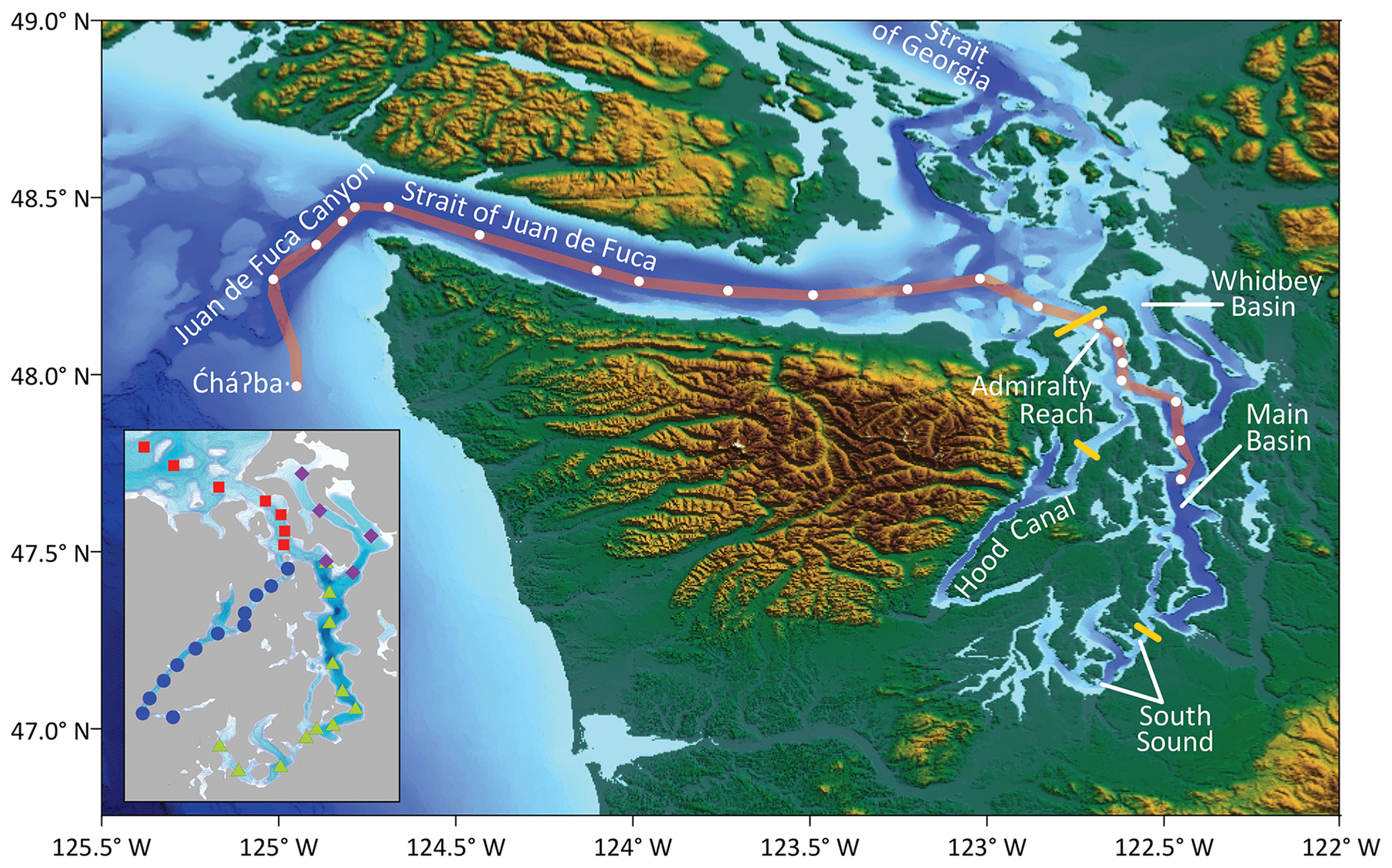
Figure 1 Map of the southern Salish Sea and its boundary waters with all study basins named. The subset of sampling stations tracing a path between the Ćhába⋅ mooring on the Washington state (USA) continental shelf and the Main Basin of Puget Sound constitute the Sound-to-Sea (S2S) transects. The inset map shows the station groupings used for the analyses of Puget Sound cruises: Admiralty Reach (AR, red squares), Main Basin–South Sound (MB–SS, green triangles), Whidbey Basin (WB, purple diamonds), and Hood Canal (HC, blue circles). Yellow dashes in the main figure denote the locations of glacial sills. Topographic and bathymetric data were extracted from the NOAA National Centers for Environmental Information Grid Extract Coastal Relief Model (3 s resolution, https://www.ncei.noaa.gov/maps/grid-extract/, last access: 13 November 2014). Data were gridded in Surfer using a minimum curve gridding technique.

2 Data collection, quality assurance, and initial quality control

Puget Sound (PS) is a glacial fjord estuary complex on the North American Pacific coast, receiving drainage from forested, agricultural, and urban landscapes. It comprises the southernmost part of the Salish Sea, which also encompasses the Strait of Juan de Fuca and the Strait of Georgia (Fig. 1). Puget Sound is comprised of four basins – Main Basin, South Sound, Whidbey Basin, and Hood Canal – as well as Admiralty Reach, a glacial sill complex defining the entrance to Puget Sound. We refer to the most ocean-influenced areas, the coast and Strait of Juan de Fuca, collectively as “boundary” waters for Puget Sound. The Strait of Juan de Fuca (SJdF), Admiralty Reach (AR), Main Basin (MB), and South Sound (SS) have well-mixed waters due to tidal and wind mixing within the basins. In contrast, Whidbey Basin (WB) and Hood Canal (HC) are narrower, and vertical mixing is inhibited by large river inputs that result in strong stratification.

The February 2008–October 2018 cruises described here are part of an ongoing Salish cruise time series, consisting of Sound-to-Sea (S2S) and Puget Sound (PS) cruises (Table 1; Alin et al., 2022) surveying physical and biogeochemical conditions throughout the water column. Semiannual S2S cruises sample a transect of stations between Seattle and the coastal ocean acidification mooring “Ćhába⋅” – meaning “whale tail” in the language of the Quileute Tribe – offshore of La Push, Washington. Seasonal PS cruises sample stations in all sub-basins of the Puget Sound, with consistent timing in April, July, and September since 2014. Of the 35 cruises, 12 occupied S2S stations, 17 surveyed Puget Sound, 4 sampled only at Ćhába⋅, and 2 cruises occupied both S2S and PS stations (Fig. 1). Surveys started during all months of the year, except June and December, with the most frequent months being April (n=5), May (5), July (5), September (7), and October (6), and one each in February, August, and November (Table 1). S2S cruises provided the opportunity to sample stations between the Main Basin of Puget Sound and coastal Washington waters adjacent to the Ćhába⋅ mooring, including the Strait of Juan de Fuca, and occurred most frequently in May (n=5) and October (5), providing early and late upwelling season snapshots in boundary waters. Puget Sound cruises have occurred most frequently in April (n=4), July (5), and September (6). The resulting cruise data set comprises 3971 samples with paired observations of inorganic carbon, nutrients, oxygen, and conductivity–temperature–depth (CTD) measurements across a complex estuary system and along the gradient from the estuary to the coastal ocean as well as up to 7525 observations lacking one or more measurements (Table 2). In this paper, we describe the methods used to produce all data in the corresponding data product.

The Salish cruises described here were preceded by semiannual Puget Sound Regional Synthesis Model (PRISM) cruises that occupied the same Puget Sound stations, typically in June and December, but the 1998–2007 PRISM cruises had not yet initiated inorganic carbon measurements and were, thus, not included in this data compilation and description (PRISM data are available at https://nvs.nanoos.org/CruiseSalish, last access: 15 September 2023). The seasonal Salish cruises (2014–2018) included in this data product and further described in Alin et al. (2023a) are ongoing, and updates to this cruise time series will be provided in follow-on papers and data products.

Table 1 Details of each cruise included in the 2008–2018 Salish cruise data product, including the cruise identification (ID), dates, contributing research programs, geographic scope of observations, ship, and funding sources.

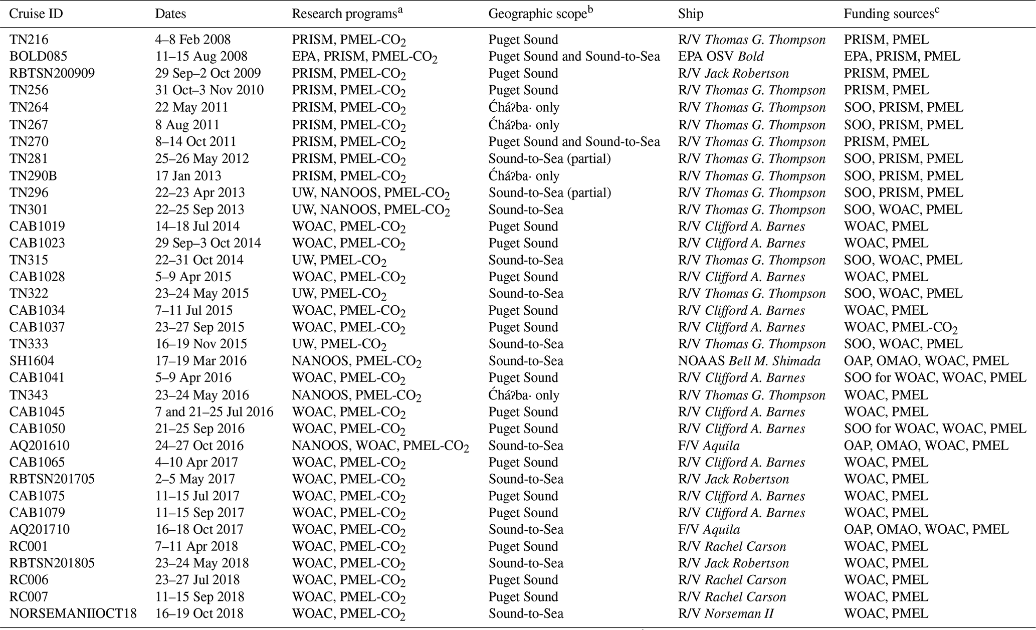
^a Research programs are those institutional programs that led the collection of the core variables described in this publication for each cruise data set. ^b Geographic scope refers to the area within Washington state marine waters that was sampled on each cruise and refers to station groupings described in Fig. 1. ^c Funding programs provided support for ship time and principal investigator, cruise participant, and laboratory or data analyst salaries. Abbreviations for research and funding programs are as follows: WOAC – Washington Ocean Acidification Center; UW – University of Washington; EPA – US Environmental Protection Agency; NOAA – US National Oceanic and Atmospheric Administration; PMEL – NOAA Pacific Marine Environmental Laboratory; PMEL-CO₂ – PMEL CO₂ Research Group; PRISM – UW Puget Sound Regional Synthesis Model; SOO – UW School of Oceanography; NANOOS – Northwest Association of Networked Ocean Observing Systems; OAP – NOAA Ocean Acidification Program; and OMAO – NOAA Office of Marine and Aviation Operations.

2.1 CTD profiles and water collection

On all cruises, we surveyed the network of either the S2S or PS sampling stations using Niskin bottles and CTD, oxygen, and additional sensors affixed to a rosette cage and deployed from a research vessel through the water column (Table 1). Downcast CTD sensor profiles were collected at each sampling station using a Sea-Bird 911plus CTD–deck box combination (except where noted in individual cruise metadata), allowing sensor data to be seen in real time. Upcast CTD data, corresponding to when the Niskin bottles on the rosette cage were fired and water samples were collected, are the focus of this publication and the corresponding data package (Alin et al., 2022). The conductivity, temperature, and pressure sensor initial accuracy errors are ±0.0003 S m⁻¹, ±0.001 ^∘C, and ±0.015 % of the full-scale range, respectively; the corresponding typical stability is on the order of 0.0003 S m⁻¹ per month, 0.0002 ^∘C per month, and 0.02 % of the full scale per year; and the corresponding master clock error contributions are 0.00005 S m⁻¹, 0.00016 ^∘C, and 0.3 dbar. CTD sensor data were processed using Sea-Bird's proprietary data processing software using the Data Conversion and Bottle Summary modules, which convert raw data from the CTD to engineering units, derive dependent variables (namely, salinity and potential density anomaly, or sigma theta, σ_θ), and write a bottle data summary to an output file. Temperatures were submitted on the International Temperature Scale of 1990 (ITS-90). Salinities in this data product were submitted on the Practical Salinity Scale (PSS-78), which is a unitless quantity but some practitioners incorrectly express it as practical salinity units (PSUs) to designate that it uses this scale (IOC et al., 2010).

Table 2 Final data variable names, descriptions, units, and measurement temperature (T) and pressure (P) conditions for observations in the Salish cruise data product.

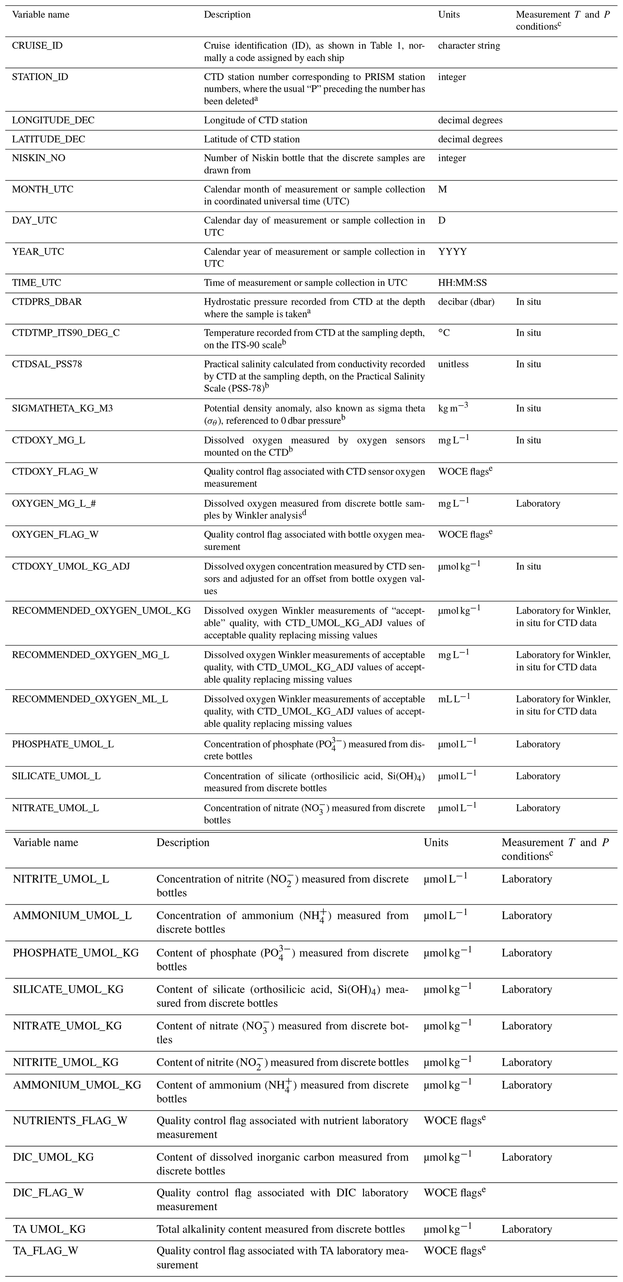
^a See http://nvs.nanoos.org/CruiseSalish (last access: 15 September 2023) for full information on locations and descriptive names for each station. ^b Measurements taken on CTD upcast at the same depth where the Niskin bottle associated with a discrete bottle measurement was closed. ^c Designations “In situ” and “Laboratory” denote the temperature and pressure conditions under which each measurement was taken. ^d In the submitted data product, Winkler oxygen measurements have some replicate samples, and the replicate number will thus be inserted in place of the “#” sign, e.g. “OXYGEN_MG_L_1”, “OXYGEN_MG_L_2”, etc. ^e World Ocean Circulation Experiment (WOCE) water sample quality flag definitions are used: 2 – acceptable value; 3 – questionable value; 4 – bad value; 5 – value not reported; 6 – mean of replicate measurements (used for DIC_UMOL_KG and TA_UMOL_KG only); and 9 – sample not drawn (Tables 4.9 and 4.10 in WOCE, 1998, for bottle and CTD data, respectively).

2.2 Dissolved oxygen

Dissolved oxygen concentration was measured by both Sea-Bird oxygen (SBE 43) sensors attached to the CTD and Winkler analyses of discrete bottle samples collected from the Niskin bottles and analyzed by University of Washington staff. The SBE 43 initial accuracy is ±2 % of saturation, with typical stability of 0.5 % per 1000 h of deployed time.

Discrete oxygen samples were always collected first from a Niskin bottle after opening it, due to the rapid air–sea gas exchange of oxygen. To collect discrete dissolved oxygen samples, a TYGON tube was attached to the Niskin bottle and flushed so that no air remained. A 125 mL iodine flask was inverted over the upward-pointing tube and flushed, rinsing and reverting the bottle to allow it to fill, overflowing 3 times its volume. The tube was withdrawn without turbulence, maintaining an overfull bottle. Reagents were prepared and added to samples as described in Intergovernmental Oceanographic Commission (1994). The flask was capped without introducing a bubble and inverted about 12 times to mix thoroughly. The bottle was allowed to settle, then remixed, and a bead of deionized water was added to the lid for an airtight seal. We collected and analyzed replicate samples from approximately 10 % of the Niskin bottles sampled.

The analysis method is based upon whole-flask titration of iodine (Carpenter, 1965; as described by Codispoti, 1988), which is produced by an equivalent amount of dissolved oxygen. The iodine flasks used for sampling, with a nominal volume of 125 mL, were pre-calibrated so that their volumes were precisely known. Samples were titrated within 1–2 d of being collected, allowing the samples to come to room temperature where the titration occurred. Discrete oxygen samples were used to validate sensor O₂ observations on the CTD package. A precision of 1 % on Winkler oxygen measurements was calculated as the average standard error on triplicate analyses.

2.3 Dissolved inorganic carbon

Inorganic carbon samples were collected from Niskin bottles immediately after oxygen samples and analyzed at the NOAA Pacific Marine Environmental Laboratory (NOAA/PMEL). An exception to the sampling order was on the August 2008 cruise, when spectrophotometric pH (on the total scale, pH_T) samples were collected between O₂ and DIC samples; however, these directly measured pH_T data are not included in this data product. A combined sample for dissolved inorganic carbon (DIC) and total alkalinity (TA) measurements was drawn into ∼540 mL borosilicate glass flasks using silicone tubing according to procedures outlined in the “Guide to Best Practices for Ocean CO₂ Measurements” (standard operating procedure, SOP, 1 in Dickson et al., 2007). Briefly, flasks were rinsed once and filled from the bottom with care not to entrain any bubbles, overflowing by at least one-half volume. The sample tube was pinched and withdrawn, creating a small headspace, and 0.2 mL of saturated mercuric chloride (HgCl₂) solution was added as a preservative. Sample bottles were then sealed with glass stoppers that were lightly covered with APIEZON L grease. Stoppers were held in place until analysis with a thick rubber band over the stopper attached to a plastic clamp around the neck of the sample flask. Sample bottles were inverted several times to ensure mixing of the HgCl₂ throughout the sample. DIC samples were collected from a variety of depths, with approximately 5 % of samples drawn in duplicate (or occasionally triplicate). All samples were stored under cool, dark conditions until analysis.

DIC concentrations were measured at PMEL on analytical systems consisting of a coulometer (UIC Inc.) coupled with a single-operator multiparameter metabolic analyzer (SOMMA) developed to extract DIC from seawater (Johnson et al., 1985, 1987, 1993; Johnson, 1992). Each coulometer was calibrated at the beginning of each analysis day, when a fresh coulometric cell was prepared, by injecting aliquots of pure CO₂ (99.999 %) via an eight-port valve (Wilke et al., 1993) outfitted with two calibrated sample loops of different sizes (∼1 and ∼2 mL). Calibration consisted of running one or more sets of gas loop injections at the beginning of each cell. Typically, 20–25 samples were analyzed per coulometric cell.

The accuracy of SOMMA measurements was determined with the use of Certified Reference Materials (CRMs), consisting of filtered and UV-irradiated seawater and supplied by the laboratory of Professor Andrew Dickson of Scripps Institution of Oceanography (SIO). Certified reference values of CRMs were determined manometrically on land at SIO. CRMs were measured near the beginning of each cell. Replicate samples were typically run throughout the life of the cell solution for quality assurance and to assess the integrity of the coulometer cell solutions. All DIC data have been corrected for dilution by the small amount of saturated HgCl₂ added and for observed offsets between PMEL measurements and certified values for the CRM batch values. An estimate of precision is provided by the replicate samples collected from approximately 5 % of the Niskin bottles sampled. The average absolute difference from the mean among replicates is typically on the order of 1.5 µmol kg⁻¹. This is consistent with our independent measurements of accuracy of the CRMs using the gas calibration loops. No systematic differences among replicates were observed, except in near-surface waters, where stratification is sufficiently strong in Puget Sound that a pair of samples collected in immediate succession from the same Niskin can have DIC (and TA) values >50 µmol kg⁻¹ apart from each other. Thus, near-surface replicate samples were not used to estimate analytical precision.

2.4 Total alkalinity

After DIC measurement on a sample, the remaining seawater in a sample bottle was analyzed at NOAA/PMEL to determine TA by acidimetric titration. The method is based upon the open-cell method described by Dickson et al. (2003; see also SOP 3b in Dickson et al., 2007), wherein the sample is first acidified to reduce sample pH to less than 3.6, followed by bubbling CO₂-free air through the sample to facilitate the removal of the CO₂ evolved by the acid addition. After removal of all carbonate species from solution, the titration proceeds until a pH of less than 3.0 is attained. Then the equivalence point is evaluated from titration points in the pH region from 3.0 to 3.5 using a nonlinear, least-squares procedure that corrects for reactions with sulfate and fluoride ions (Dickson et al., 2003). Titration progress is monitored by measuring the electromotive force of a combination glass–reference electrode. Instrument control and data acquisition occur via custom software developed by Andrew Dickson's laboratory at SIO. Typical titrations were completed in 10–14 min and required 20–24 acid additions to reach a pH of 3.0.

Titrations were carried out in water-jacketed, 250 mL beakers to ensure temperature stability. The temperature of the samples and the beakers was controlled by use of a refrigerated recirculating water bath. Seawater samples were measured gravimetrically (105–135 g depending on salinity) to ensure that a sufficient number of titration points were achieved (typically 18–22). A Metrohm Dosimat 765 was used to deliver certified acid titrant to the sample beaker in small, precise increments (0.04–0.05 mL depending on sample size and salinity). The acid titrant used was 0.1 mol kg⁻¹ hydrochloric acid prepared in 0.6 mol kg⁻¹ sodium chloride to approximate the ionic strength of seawater (0.7 mol kg⁻¹). The titrant was coulometrically analyzed and certified by Andrew Dickson's laboratory.

Analytical accuracy was assessed by periodic analysis of the same CRMs as used for DIC. No corrections were made for offsets between the certified and measured CRM values when the offset was below 2 µmol kg⁻¹; the difference from accepted and measured CRM values was added or subtracted from measured sample values for offsets between 2 and 4 µmol kg⁻¹; and above 4 µmol kg⁻¹, instruments were not run until repaired. Precision was monitored by analyzing replicates drawn from approximately 10 % of the Niskin bottles sampled.

2.5 Nutrients

One bottle sample for nutrients was collected from each Niskin after oxygen and inorganic carbon bottle samples had been collected, for subsequent analysis of phosphate, silicate, nitrate, nitrite, and ammonium concentrations at the Marine Chemistry Laboratory at the University of Washington (UW) School of Oceanography. To collect samples, a 60 mL high-density polyethylene (HDPE) syringe was prepared by removing the plunger and attaching a Nalgene filter (surfactant-free cellulose, 25 mm, 0.45 µm pore size). The plunger and the inside of the syringe were rinsed three times using seawater from the Niskin bottle. The syringe was then filled with sample water from the Niskin, and the plunger inserted. About 1 mL of sample water was filtered through the filter, then about 5–10 mL of sample was dispensed into the 60 mL HDPE sample bottle to rinse the bottle and cap, with the rinse water then discarded. Rinsing was repeated three times. Next, about 45 mL of sample was filtered into the sample bottle, such that it was approximately two-thirds full. The cap was secured and the bottle frozen upright until analysis.

Analyses and calibration followed the protocols of the World Ocean Circulation Experiment (WOCE) Hydrographic Program (Intergovernmental Oceanographic Commission, 1994) using a SEAL Analytical AA3 in the UW Marine Chemistry Laboratory (accreditation codes can be seen in University of Washington, 2021). Minimum detection limits were 0.04 µM for phosphate, 0.23 µM for silicate, 0.29 µM for nitrate, 0.01 µM for nitrite, and 0.05 µM for ammonium.

2.6 Uncertainty of oceanographic measurements

Overall temperature and salinity uncertainties are ±0.01 ^∘C and ±0.02, respectively. Oxygen measurement uncertainties were ±2 % of saturation on CTD oxygen measurements and precision of 1 % on Winkler oxygen measurements. Measurement uncertainties were ±0.1 % (∼2 µmol kg⁻¹) on DIC and TA measurements. Uncertainty on nutrient measurements were ±2 %. However, it should be noted that the uncertainties given above reflect analytical uncertainties for discrete biogeochemical measurements (Winkler O₂, DIC, TA, and nutrient analyses) but cannot capture the uncertainty associated with field sampling or sample handling errors (e.g., Niskin bottles firing at the wrong depth or samples incorrectly preserved or stored).

3 Unit conversions and data quality control

All unit conversions and extended primary quality control (QC) measures are described in this section. All measurements were subjected to quality assurance (QA) measures in the laboratory, as described in Sect. 2, as well as quality control measures immediately following analysis, which reflect instrument diagnostic information and other observations of measurement quality and sample integrity made in the laboratory. Initial QC flags were assigned on the basis of laboratory instrument diagnostics only for DIC and TA analyses based on the WOCE water sample quality flag definitions listed in the footnotes of Table 2. Here, we describe the calculations undertaken to convert units to prepare for subsequent analyses of derived inorganic carbonate system parameters necessary for understanding ocean acidification, such as calcium carbonate saturation states (Ω), pH_T, partial pressure or fugacity of CO₂, and Revelle factor, using CO2SYS (e.g., Lewis and Wallace, 1988; van Heuven et al., 2011; Pelletier et al., 2007), the R package seacarb (Gattuso et al., 2023), or other water chemistry calculation programs.

We also detail the extended QC procedures undertaken to ensure that only the highest-quality data were archived and used to generate depth transects. However, because of the tremendous natural variability in this region and the occurrence of strong environmental anomalies during the decade of observations in the data product, we took the approach of flagging data points that may ultimately end up being deemed “bad” measurements (QC flag of 4) as “questionable” (QC flag of 3) to indicate that they deserve further attention by other investigators. Good measurements are marked with a QC flag of 2.

3.1 Calculated and adjusted variables

Temperature-independent units are required for carbonate system calculations (Lewis and Wallace, 1988; Gattuso et al., 2023) and are consistent with the recommendations of Jiang et al. (2022). Specifically, in order to make carbonate system calculations, phosphate and silicate data were converted to temperature-independent units of micromoles per kilogram for compatibility with the chemical dissociation constants used in seacarb or CO2SYS calculations. Throughout this article, we discuss results using temperature-independent units of micromoles per kilogram, referred to as “substance content” rather than concentration, which has milligram-per-liter or micromole-per-liter units. However, the publicly accessible Salish cruise data product includes all parameters in original units as well as those converted to micromole-per-kilogram units for oxygen, phosphate, and silicate concentrations to enable use of this data package with internally consistent units by diverse end users.

3.1.1 Potential density anomaly, or sigma theta (σ_θ), calculations

Potential density (ρ_θ) values, which represent the density of seawater calculated with in situ salinity, potential temperature, and pressure referenced to 0 dbar, were calculated using the 2010 thermodynamic equations of state of seawater (IOC et al., 2010). Potential density (units of kg m⁻³) is necessary for converting units from per-liter “concentration” to per-kilogram basis “content” units, as is conventional in chemical oceanography. The potential density anomaly, or sigma theta (σ_θ), is a useful way of comparing the relative densities of different water masses across space, depth, and time; it is provided with the data product but not discussed further in this article, as it tracks salinity closely in Puget Sound. σ_θ is calculated simply as follows:

$$\begin{array}{}\text{(1)}& {\mathit{\sigma }}_{\mathit{\theta }}={\mathit{\rho }}_{\mathit{\theta }}-\mathrm{1000}.\end{array}$$

It is also expressed in units of kilograms per cubic meter.

3.1.2 Oxygen unit conversions

All CTD and bottle dissolved oxygen (O₂) data were converted from original units (mg O₂ L⁻¹ seawater) to micromoles of O₂ per kilogram of seawater using Eq. (2):

$$\begin{array}{}\text{(2)}& {\mathrm{O}}_{\mathrm{2}}\left(\text{in }\mathrm{\mu }\mathrm{mol}{\mathrm{kg}}^{-\mathrm{1}}\right)={\displaystyle \frac{{\mathrm{O}}_{\mathrm{2}}\left(\text{in }\mathrm{mg}{\mathrm{L}}^{-\mathrm{1}}\right)\times \mathrm{44}\mathrm{659.6}}{{\mathit{\rho }}_{\mathit{\theta }}\times \mathrm{1.42903}}},\end{array}$$

where ρ_θ is in units of kilograms per cubic meter, as noted above, and 44 569.6 is the reciprocal of the molar volume of O₂ gas, in micromoles per liter (from 22 391.6 cm³ mol⁻¹ in García and Gordon, 1992). Conversion factors of 1000 L m⁻³ in the numerator and 1000 mL L⁻¹ in the denominator cancel out. For end users preferring O₂ data in units of milliliters per liter, we also provide the final, recommended O₂ values (Sect. 3.1.4) in milliliters per liter in the submitted data product using the conversion:

$$\begin{array}{}\text{(3)}& {\mathrm{O}}_{\mathrm{2}}\left(\text{in }\mathrm{mL}{\mathrm{L}}^{-\mathrm{1}}\right)={\displaystyle \frac{{\mathrm{O}}_{\mathrm{2}}\left(\text{in }\mathrm{mg}{\mathrm{L}}^{-\mathrm{1}}\right)}{\mathrm{1.42903}\left(\text{in }\mathrm{mg}{\mathrm{mL}}^{-\mathrm{1}}\right)}},\end{array}$$

where the conversion factor can be derived from García and Gordon (1992), although a Sea-Bird technical document (Sea-Bird Electronics, 2013) is also often cited.

3.1.3 Density corrections for measurements conducted in laboratory

Nutrient data were also converted to units of micromoles per kilogram to facilitate subsequent calculations in CO2SYS or seacarb. To do so, the density of seawater under laboratory conditions was calculated following the TEOS-10 thermodynamic equation of seawater (IOC et al., 2010), using 22 ^∘C for laboratory temperature, 0 dbar pressure, and in situ salinity. After converting density to units of kilograms per liter (from kg m⁻³), nutrient concentration measurements in micromoles per liter were converted to micromoles per kilogram by dividing by the calculated laboratory seawater density. Nutrient measurements are submitted in both micromole-per-liter (original units) and micromole-per-kilogram forms to facilitate CO2SYS and seacarb calculations and other end uses.

3.1.4 Adjusting CTD oxygen measurements for offset from bottle oxygen values

We plotted Winkler/bottle O₂ (OXYGEN_UMOL_KG, y axis) against CTD O₂ (CTDOXY_UMOL_KG, x axis) values in micromoles per kilogram separately for each cruise to determine offset and slope corrections between the two sets of measurements through linear regression. Prior to regression, we inspected all visually apparent outliers in the context of the depth profiles at each station. Oxygen quality flags were not assigned at the time of analysis, although notes were taken on any problems encountered at the time of analysis (e.g., bubbles in titrator or running out of reagent). Samples that had analytical problems noted or that were collected from deep water and had outlying bottle O₂ values were flagged 4, as these values are likely bad for any application, and were not included in the data product. The data labeled with a 4 were identified from samples collected from water depths >25 m with O₂ concentrations that appeared to be from a substantially different depth within a given profile, whether the value appeared to be substantially too low or too high.

Another subset of samples was identified as having mismatches between CTD and bottle O₂ values but where neither value was necessarily bad. These bottle samples were flagged 3 in the submitted data sets, representing questionable data, to denote the mismatch between bottle and CTD measurements. Most of these were collected near the surface and likely just reflect strong stratification resulting in real differences in the O₂ concentrations measured by the CTD O₂ sensor compared with those in the overlying Niskin bottle sample.

All other samples were presumed to be of acceptable quality and assigned initial QC flags of 2 accordingly. All samples flagged 3 or 4 during inspection were excluded from the regression to avoid introducing leverage into the resulting regression equation; however, many of the samples flagged with values of 3 may be good for other applications. In total, 178 CTD–bottle O₂ pairs were excluded due to having assigned data quality flags of 3 or 4 out of a total of 6153 pairs (<3 %; Table 3).

Table 3 Oxygen correction coefficients and statistics for each cruise.

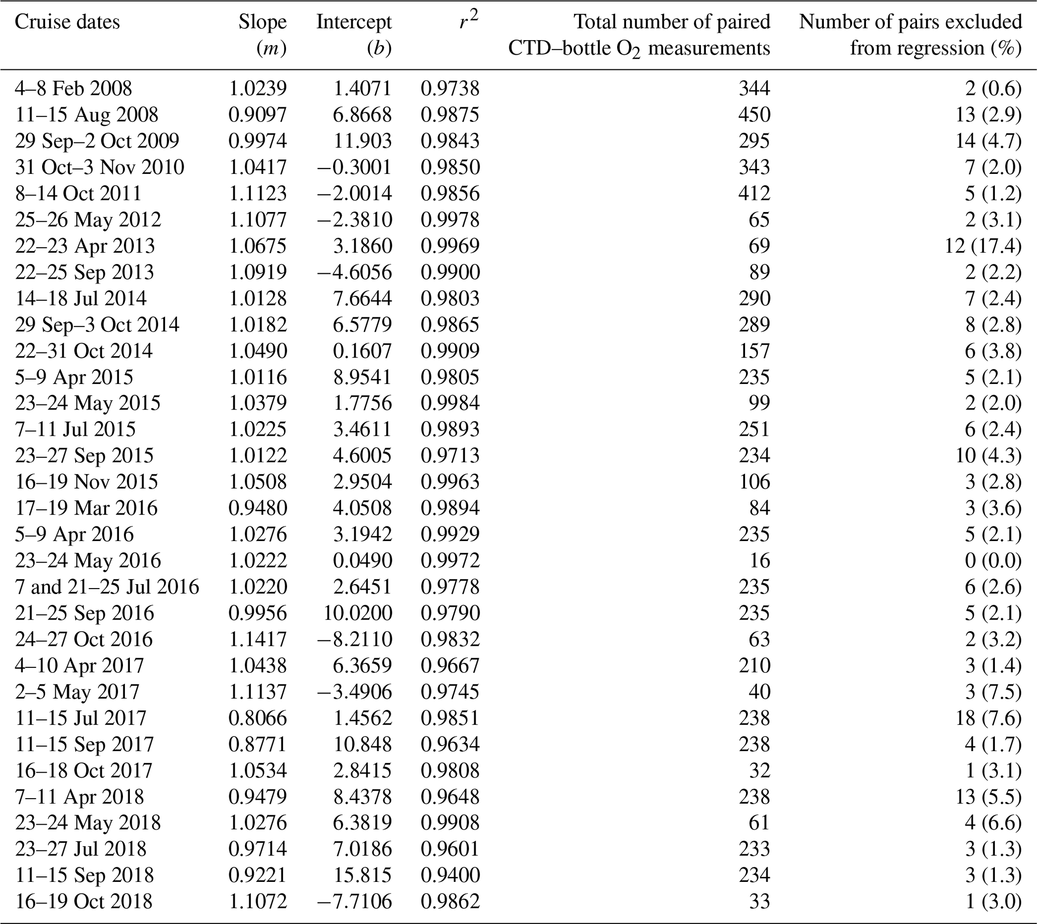
With the remaining data points, we generated linear regression equations for each cruise (all regression r² values were ≥0.94) and used this relationship to adjust the CTD O₂ data for the offset and slope differences from bottle O₂ values. In other words, while we had bottle O₂ data for a subset of all Niskin bottle samples, we generated the bottle-O₂-equivalent value for all CTD O₂ samples by applying the regression relationship to the CTD O₂ data. Coefficients from linear regressions used to adjust CTD O₂ values for all cruises are listed in Table 3 and correspond to the following equation:

$$\begin{array}{}\text{(4)}& \mathrm{CTDOXY}\mathrm{\_}\mathrm{UMOL}\mathrm{\_}\mathrm{KG}\mathrm{\_}\mathrm{ADJ}=m\times \text{CTDOXY\_UMOL\_KG}+b,\end{array}$$

where m is the slope and b is the intercept of the regression equation between the Winkler (OXYGEN_UMOL_KG) and CTDOXY_UMOL_KG values (Table 3). The CTDOXY_UMOL_KG_ADJ variable in the submitted data files represents the CTD oxygen values adjusted in this manner. Regression slope values ranged from 0.81 to 1.14, with intercepts from 0.05 to 15.8 µmol kg⁻¹.

Finally, we created a hybrid oxygen column consisting of all Winkler O₂ data with “acceptable” quality, with CTDOXY_UMOL_ KG_ADJ filling missing values; this parameter is called RECOMMENDED_OXYGEN_UMOL_KG. The recommended O₂ data column is also provided in both milligram-per-liter and milliliter-per-liter units to facilitate adoption by various end user communities. The conversion of recommended O₂ values from micromoles per kilogram to milligrams per liter and milliliters per liter was done by rearranging Eqs. (2) and (3).

3.2 Extended quality control

Extended quality control consisted of the preparation of property–property plots after any samples flagged as a 4 (bad value) were eliminated and interpolated pressure vs. along-transect-distance plots (or “depth-transect plots”). Property–property plots were made of parameters that normally show strong correlations with each other (Figs. 2, 3). Following the recommendations of Jiang et al. (2021) for CODAP-NA data sets, we prepared the following plots: (1) CTD salinity against CTD temperature, (2) TA against CTD salinity, (3) TA against silicate content, (4) TA against DIC, (5) DIC against adjusted CTD oxygen content, (6) phosphate against nitrate, (7) nitrate against silicate, and (8) all nutrients (silicate, phosphate, nitrate, nitrite, and ammonium) against adjusted CTD oxygen content. Outliers were again compared to nearby depth and station samples within their cruise and flagged as 3 or 4 as appropriate. All data in the Salish cruise data product with QC flags of 3 were excluded from statistical summaries. However, their distributions are retained in gray in property–property plots to provide end users with more information about how likely the data are to be useful for their applications (Figs. 2, 3).

Interpolated depth transects prepared in Golden Software's Surfer program visually depict cross-sections of oceanographic parameters along transects from the coast into Puget Sound for S2S cruises (Fig. 4) and from Admiralty Reach along transects toward the terminus of each basin for Puget Sound cruises (Figs. 5–9). Outliers identified on depth-transect plots typically manifest as a “bullseye” pattern corresponding to a single sample. Bullseye points were evaluated and reassigned a quality flag of 4 if it was ascertained that the value was likely bad (e.g., due to a Niskin bottle firing at the wrong depth or a sample bottle having been improperly preserved or sealed between collection and analysis) rather than a correctable data entry error. Outliers that changed distributions of oceanographic parameters in the depth transects were subsequently excluded from the cross-sections.

Offsets due to strong stratification in surface waters may yield apparent outliers in such property–property plots comparing CTD sensor data with Niskin bottle analysis data or bottle samples collected sequentially (e.g., Winkler O₂ vs. DIC, TA, or nutrients). In the property–property plots described above, salinity and temperature are based on sensor measurements associated with the CTD package; oxygen data were derived from both CTD sensor and bottle measurements; and DIC, TA, and nutrient measurements were conducted on bottle samples collected some distance above the CTD sensors. While both sensor and discrete bottle sample data in such comparisons may represent accurate measurements, particularly in stratified surface waters, we applied quality flags of 3 (questionable) to the Niskin data of disagreeing sample pairs to reflect the fact that the CTD–bottle sample pairs may not be suitable for all end uses (e.g., as described in Sect. 3.1.4). For instance, using paired sensor and bottle data from strongly stratified surface waters could yield unreliable empirical relationships (cf. Alin et al., 2012; Fassbender et al., 2017).

4 Results

4.1 Sampling coverage and extended quality control of the 2008–2018 Salish cruise data product

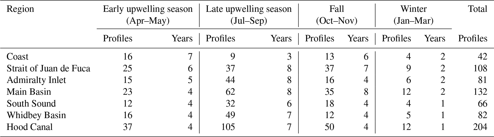
To differentiate the distributions of physical and biogeochemical parameters across seasons in the Salish cruise data product, we defined four seasons as fall (October–November), winter (January–March), early upwelling season (April–May), and late upwelling season (July–September) (months not listed were not sampled on cruises included in the 2008–2018 Salish cruise data product). Collectively, the 2008–2018 Salish cruise data product includes oceanographic observations from 715 profiles, with 144 profiles collected during the early upwelling season, 338 during the late upwelling season, and 181 during fall (Table 4). As in many regions, the fewest cruise observations were collected during winter conditions (52 profiles) (e.g., Benway et al., 2016; Jiang et al., 2021). Late-upwelling-season profiles occurred during more years across the cruise time series than during early-upwelling-season or fall months, and profiles collected during winter months only occurred during 1–2 years in any basin. Across the region, the fewest profiles in this data product were collected in coastal waters. The largest number of profiles were collected in Hood Canal, which received the most sampling effort due to the need to understand variability in oxygen and acidification conditions in this location that is known to experience recurring seasonal hypoxia.

Table 4 Numbers of water column profiles and years sampled in each basin by season. Months sampled in each season are indicated in each column header.

Sensor measurements of temperature, salinity, and oxygen are the most numerous observations across the Salish cruise profiles (n=7525, 7525, and 7491, respectively), and very few of these measurements reflected questionable values (i.e., QC flags of 3, with 3, 29, and 9 total observations, respectively) (Table 5). A few CTD profiles appeared to have higher-than-expected salinity values throughout the water column and received QC flags of 3, while individual measurements near the surface flagged as 3 (questionable) may simply reflect strong near-surface stratification and be valid measurements.

Table 5 Numbers of high-quality measurements (QC flags of 2 or 6) in the Salish cruise data product, by basin, for temperature (T, ITS-90), salinity (S, PSS-78), adjusted CTD oxygen (CTD O₂), discrete (“Winkler”) O₂, dissolved inorganic carbon (DIC), total alkalinity (TA), and nutrients. Numbers of measurements of questionable quality (QC flags of 3) that are included in the data product and may be useful for some applications are indicated in parentheses.

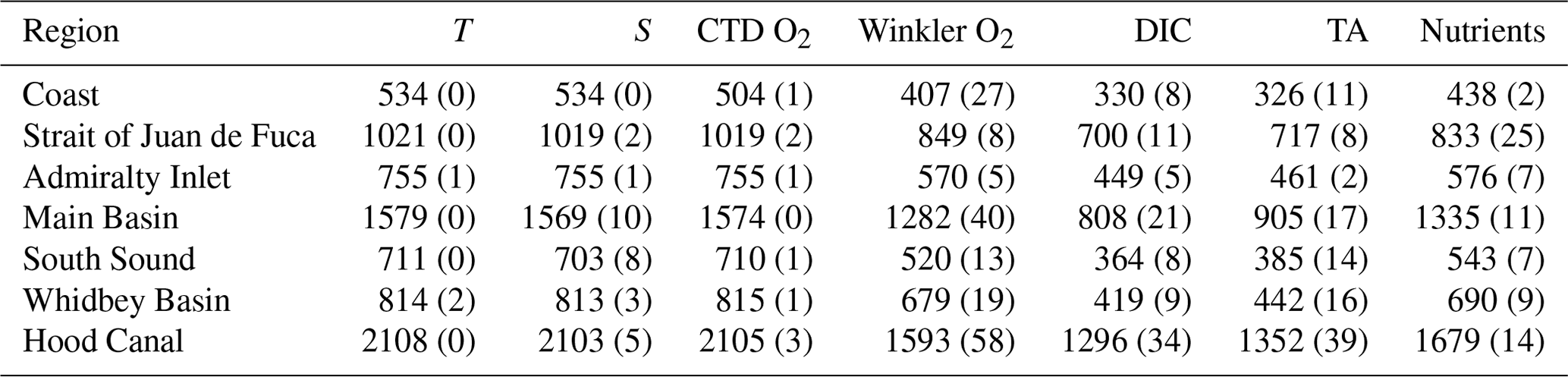
Discrete measurements of oxygen via Winkler titration were conducted on 6070 samples. Of these, 170 Winkler O₂ values were assigned QC flags indicating questionable quality and eight were flagged 4, indicating bad-quality measurements that were not submitted (reflected as QC flags of 5, meaning “not reported” in the data product) (Table 5, Fig. 2a). Of the questionable-quality samples, 74 % were shallower than 23 dbar, with 65 % in the top 12 dbar of the water column. Most Winkler O₂ data with flags of 3 also likely reflect strong near-surface stratification rather than truly questionable measurements (as explained in Sect. 3.2 and tallied in Table 3). Jiang et al. (2021) also observed near-surface sample mismatches between discrete and CTD O₂ measurements in coastal data sets and concluded that these samples likely reflected true differences between conditions measured by CTD sensors and bottle oxygen samples measurements due to slight differences in depth and strong near-surface stratification.

Dissolved inorganic carbon and total alkalinity measurements (n=4462 and 4695, respectively) received the most thorough initial QA $/$ QC attention (following the SOPs in Dickson et al., 2007), having been assigned QC flags immediately after laboratory analyses were conducted based on instrument diagnostics (with 90 and 101 QC = 3 flags assigned to DIC and TA at this stage) or routine plots generated in the process of finalizing the data (Table 5). Additional questionable QC flags were assigned during extended QC to six samples each for DIC and TA, with some overlap, based on property–property plots against salinity.

Nutrient analyses were conducted on 6169 samples (Table 5). These cruises did not have nutrient sensors, and nutrient data were not QC flagged by the laboratory providing the data. We assigned 150 nutrient observations QC flags of 3, using the property–property plots recommended by Jiang et al. (2021) to identify outliers (Fig. 2b–h). While a number of these plots showed significant scatter, we took a conservative approach to flagging outliers, assigning no flags of 4, with the recognition that many of these outliers may reflect either freshwater influence or redox or biological conditions caused by environmental anomalies such as the marine heatwave conditions of 2014–2016 (e.g., Alin et al., 2023a). Thus, we suggest that other apparent nutrient outliers deserve further scrutiny before concluding that they are necessarily questionable or bad measurements. We flagged all nutrients as questionable when only one parameter may have been an outlier, with the rationale that the full suite of nutrient measurements for that sample may warrant further attention.

In total, the Salish cruise data product consists of 3971 observations for which the full suite of inorganic carbon, oxygen, nutrient, and CTD measurements are available, with all parameters having QC flags of 2 or 6 after extended QC, indicating acceptable-quality measurements. These highest-quality, co-located measurements are the core of the Salish cruise data product most suitable for assessing multiple-stressor conditions, such as co-occurring marine heatwaves, hypoxia, and ocean acidification. This subset of the data can be used without further modification for CO2SYS or seacarb calculations and is provided as a separate CSV data product for end users wishing to perform CO₂ system calculations without having to further consider data that may be questionable. For end users who prefer to either apply average nutrient concentrations or zero values for nutrient measurements that are missing or flagged for calculating the full CO₂ system, there are an additional 305 sets of observations of DIC, TA, temperature, and salinity (with 50 of these having questionable nutrient values that may be found to be of acceptable quality after further analysis). Finally, for end users with the capacity to conduct additional QC, especially on nutrient measurements, and/or interpolate any of the missing values for a desired analysis, the full data set of 7525 observations, including measurements with QC flags of 3, is also available. All three subsets of the Salish cruise data product are available on the NOAA National Centers for Environmental Information web site, as described in Sect. 7.

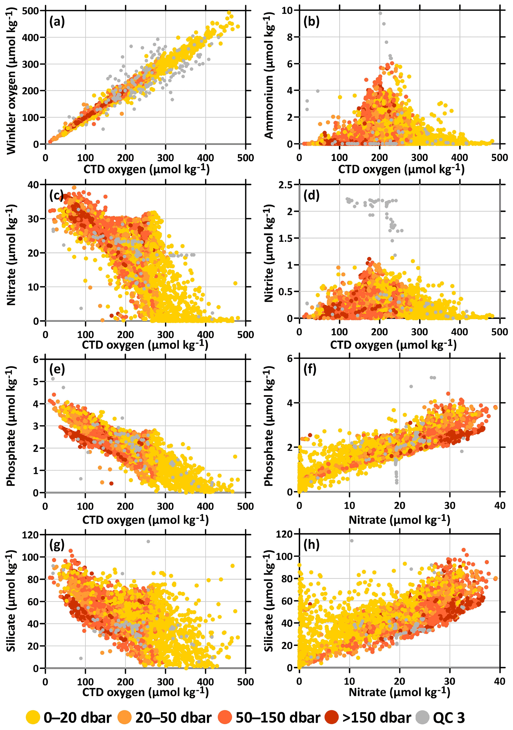
Figure 2 Property–property plots of oceanographic parameters used to detect data with potential sampling or analytical problems: (a) adjusted CTD oxygen (CTDOXY_UMOL_KG_ADJ) vs. Winkler oxygen (OXYGEN_UMOL_KG) content; (b) adjusted CTD oxygen vs. nitrate (NITRATE_UMOL_KG) content; (c) adjusted CTD oxygen vs. nitrite (NITRITE_UMOL_KG) content; (d) adjusted CTD oxygen vs. ammonium (AMMONIUM_UMOL_KG) content; (e) silicate (SILICATE_UMOL_KG) vs. total alkalinity (TA_UMOL_KG) content; (f) dissolved inorganic carbon (DIC_UMOL_KG) vs. nitrate content; (g) phosphate (PHOSPHATE_UMOL_KG) vs. nitrate content; and (h) silicate. Measurements with QC flags of 2 (acceptable) for both parameters are colored by pressure, and those with flags of 3 (questionable) for either parameter are shown in gray.

4.2 Range and spatial distribution of oceanographic conditions across the Salish cruise study region

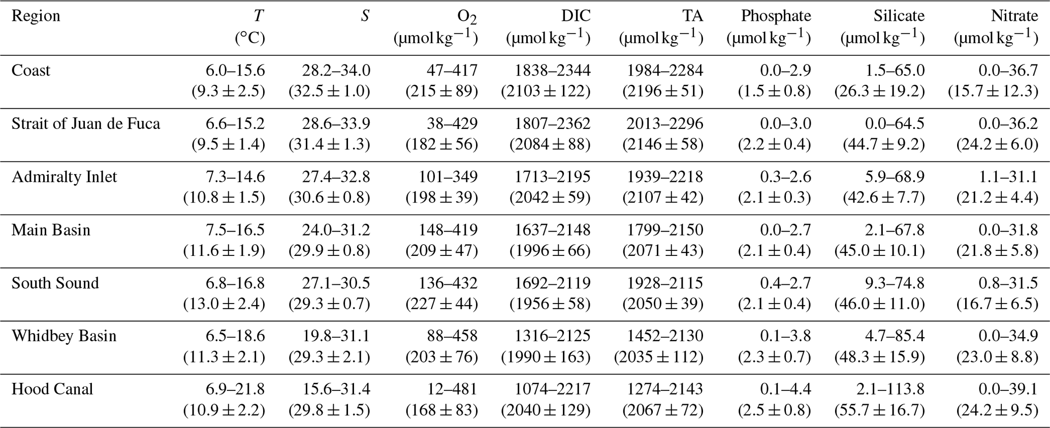
Oceanographic parameters spanning the region from Washington's coastal waters to the interior parts of each sub-basin of the southern Salish Sea occupied broad ranges of values. Summary statistics are provided in Table 6, although it should be noted that observations in this discrete sample data product are biased toward shallower depths: 40 % of observations were collected from ≤20 dbar and 63 % from ≤50 dbar, compared with 31 % from >50–150 dbar and <7 % from >150 dbar (see symbol color in Fig. 2). Parameters were often distributed similarly across boundary water stations (coast, Strait of Juan de Fuca), Puget Sound stations from more well-mixed basins (Admiralty Reach, Main Basin, and South Sound), and more stratified Puget Sound stations (Whidbey Basin and Hood Canal), but summary statistics are provided in Table 6 by individual basin. Temperatures across the region and water column spanned 6.0–21.8 ^∘C, with the lowest measurements in deep coastal waters and the highest in Hood Canal surface waters (Figs. 2; 3e, i; 4; 5). Salinity spanned 15.6–34.0, with all but two of the acceptable salinity values <25 occurring in the stratified WB and HC basins, and the highest salinity in deep coastal waters (Figs. 3e, i; 4; 6). Adjusted CTD O₂ values had their lowest and highest values in Hood Canal's deep and surface waters, respectively, spanning 12–481 µmol kg⁻¹ overall (Figs. 3h, l; 4; 9). Both DIC and TA had their minimum observations in HC surface waters (1074 and 1274 µmol kg⁻¹, respectively), while their maxima occurred in SJdF deep waters (2362 and 2296 µmol kg⁻¹, respectively), likely reflecting canyon-enhanced upwelling via the Juan de Fuca Canyon (Figs. 3g, k; 4; 7; 8). Minimum phosphate measurements approached zero in all areas, with maxima of 2.6–3.0 µmol kg⁻¹ in all basins except in WB and HC, where maxima reached 3.8–4.4 µmol kg⁻¹ (Table 6, Figs. S1–S2). Silicate content had wide ranges across the region, with the lowest minimum values of 0.0–1.5 µmol kg⁻¹ in boundary waters and the highest maxima of 85.4–113.8 µmol kg⁻¹ in WB and HC (Figs. S1–S3). Nitrate content had similar ranges across the region, with minima of 0.0–1.1 µmol kg⁻¹ and maxima spanning 31.1–39.1 µmol kg⁻¹ (Figs. S1–S4).

Table 6 Summary statistics (minimum–maximum (median ± standard deviation)) for temperature (T, ITS-90), salinity (S, PSS-78), adjusted CTD oxygen (O₂), dissolved inorganic carbon (DIC), total alkalinity (TA), phosphate, silicate, and nitrate by basin.

Across the decade-long cruise time series, separation in the seasonal and spatial distributions of the core parameters of temperature, salinity, TA, DIC, and oxygen – which are the most critical for assessing variations in marine heat, hypoxia, and acidification – can be visualized to more fully delineate the distinct water mass characteristics across the region using depth transects (Figs. 4–9). Late-upwelling-season and fall temperatures were higher than those in winter and the early upwelling season, with the broadest salinity ranges observed during the upwelling season (Figs. 3, 4). Together, the T–S distributions were widest, with the greatest scatter in both T and S values in the stratified basins, with more concentrated T and S values in the middle of the full range in the well-mixed PS regions, and most of the highest S, lowest T values clustering in boundary waters (Fig. 3–5).

For the most part, the relationship between salinity and alkalinity was linear and overlapped across seasons, basins, and depths (Figs. 3–4 and 6–7), but fall and winter mostly had higher values of both S and TA, while upwelling season TA and S occupied the full range of values seen in both parameters, with wider scatter at low S and TA values reflecting the input of rivers with a wide range of TA end-member values (e.g., Voss et al., 2014; Banas et al., 2015; Bianucci et al., 2018; Moore-Maley et al., 2018). Spatially, boundary waters more typically had high TA and S values, well-mixed PS basins had moderate values, and stratified PS basins had the lowest TA and S values (Figs. 3, 4, 6, 7).

Overall, DIC and alkalinity had a less linear relationship across the region (Fig. 3) than salinity and alkalinity. The highest DIC and TA values were observed across seasons in boundary waters and appeared to have a shallower and more linear slope than Puget Sound basins. Within PS, the more stratified basins had the broadest, least linear relationship, with a distinct flattening of TA values at the highest DIC values in stratified basins, which occurs during the late upwelling season into fall, when DIC accumulations are relatively high there (Feely et al., 2010; Alin et al., 2023a). Depth transects show that the magnitudes of seasonal changes in TA are not as large as the seasonal changes in DIC in the deep waters of the stratified basins, particularly in HC (Figs. 7, 8).

The seasonal consumption of oxygen and the enrichment of DIC by respiration drive the development of hypoxic and acidified conditions in the region (Feely et al., 2010, 2024). The relationship between DIC and O₂ is linear over the high-DIC, low-O₂ end of the distribution, across seasons and basins, reflecting the stoichiometric linkage between CO₂ and O₂ via respiration processes (Fig. 3d, h). The greater scatter among higher-O₂, lower-DIC observations, which occur in surface waters, reflects in part that O₂ and CO₂ have vastly different gas exchange rates with the atmosphere (Wanninkhof, 2014), which reduces the linearity of the relationship between CO₂ and O₂ typically seen in subsurface waters (Fig. 3l). Higher DIC and lower O₂ values tend to occur during the late upwelling season through winter across the region (Figs. 3, 8, 9). The distribution of DIC values relative to O₂ content also differs between the coast and Puget Sound, with boundary water stations having higher DIC for the same O₂ levels compared with Puget Sound basins, with stratified basins having the lowest DIC relative to O₂ levels (Fig. 3h). The most hypoxic and acidified conditions observed in the region covered by this data compilation typically occur at the southern end of HC (Feely et al., 2010; Alin et al., 2023a). In addition to the important role that respiration plays in creating the hypoxic, acidified conditions seen in the southern HC, mixing and river input contribute to the separation of the DIC vs. O₂ data distribution on the coast vs. in Puget Sound. Strong mixing of deep upwelled marine water entering Puget Sound through Admiralty Reach with river-influenced surface waters both equilibrates O₂ from deep waters with the atmosphere more than it equilibrates CO₂ (sensu Ianson et al., 2016) and mixes surface water with relatively high O₂ and low DIC and TA content from regional rivers to depth. Further mixing occurs as denser incoming marine waters transit another glacial sill going from Admiralty Reach into Hood Canal. Together, these processes contribute to lower PS DIC and TA and higher O₂ in deep PS waters, particularly in HC, compared with upwelled coastal waters. The highest O₂ and lowest DIC conditions occur in surface waters predominantly during the upwelling season, again with lower DIC for the same O₂ level in PS basins than along the coast. Mixing during winter provides nutrient supply to the surface water during spring and summer; this, coinciding with longer day lengths, fuels production that is subsequently respired at depth (Figs. S1–S4 show distributions of the major nutrients phosphate, silicate, and nitrate through the study region and seasons). The hypoxic, acidified waters from the deep HC are often pushed up to mid-depth during fall if the seasonal oceanic intrusion is denser (e.g., HC panels from October 2010 and September 2018 in Figs. 8 and 9).

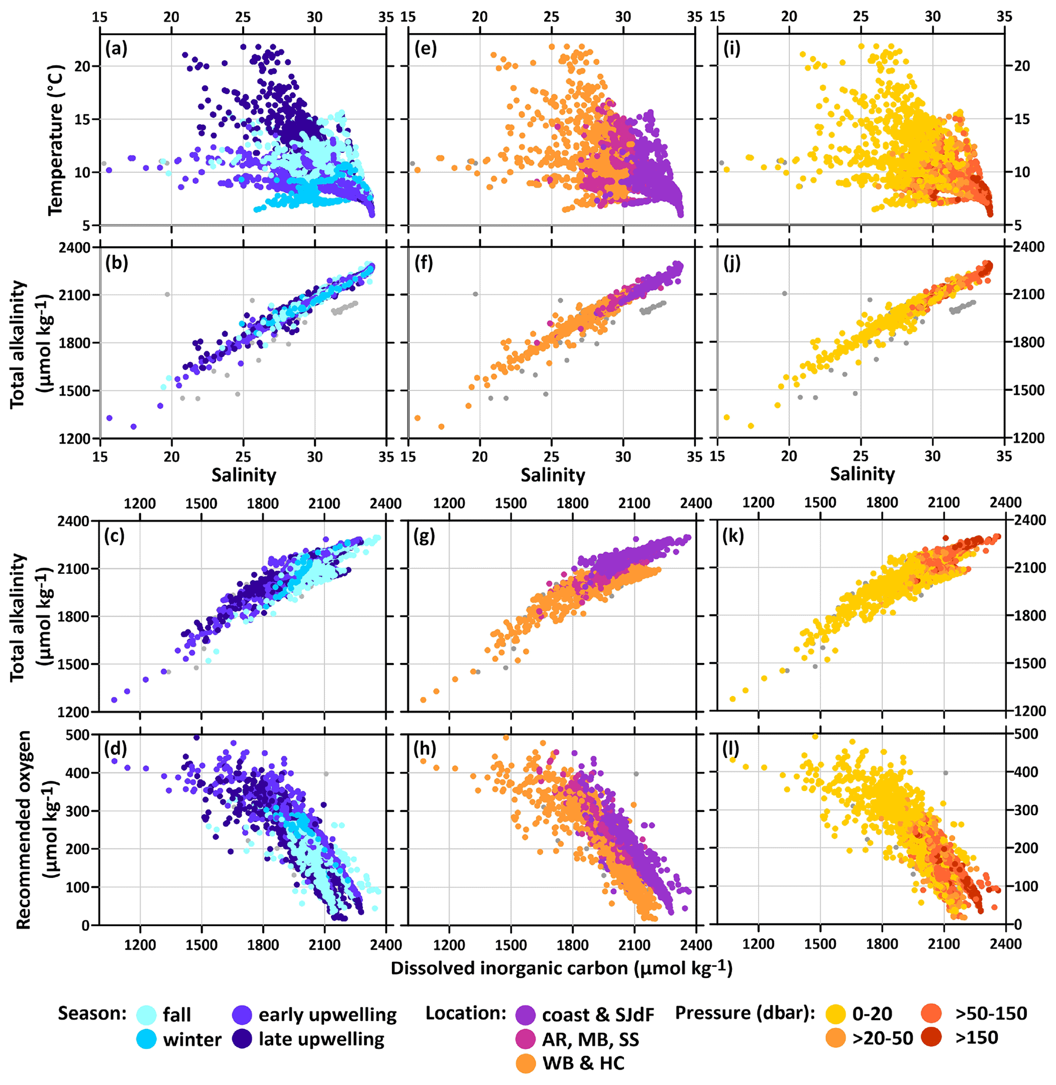
Figure 3 Property–property plots of oceanographic parameters used to delineate spatial, seasonal, and depth variability: salinity (CTDSAL_PSS78) vs. temperature (CTDTMP_DEG_C_ITS90) by season (a), location (e), and pressure (∼ depth, i); salinity vs. total alkalinity (TA_UMOL_KG) by season (b), location (f), and pressure (j); dissolved inorganic carbon (DIC_UMOL_KG) vs. total alkalinity by season (c), location (g), and pressure (k); and CTD oxygen (CTDOXY_UMOL_KG_ADJ) vs. dissolved inorganic carbon by season (d), location (h), and pressure (l). Seasons are fall (October–November), winter (January–March), early upwelling (April–May), and late upwelling (July–September). Stations are colored separately for boundary waters (coast and Strait of Juan de Fuca (SJdF)), well-mixed Puget Sound (Admiralty Reach (AR), Main Basin (MB), and South Sound (SS)), and stratified Puget Sound basins (Whidbey Basin (WB) and Hood Canal (HC)). All observations with a QC flag of 3 (questionable) for either parameter are shown in gray.

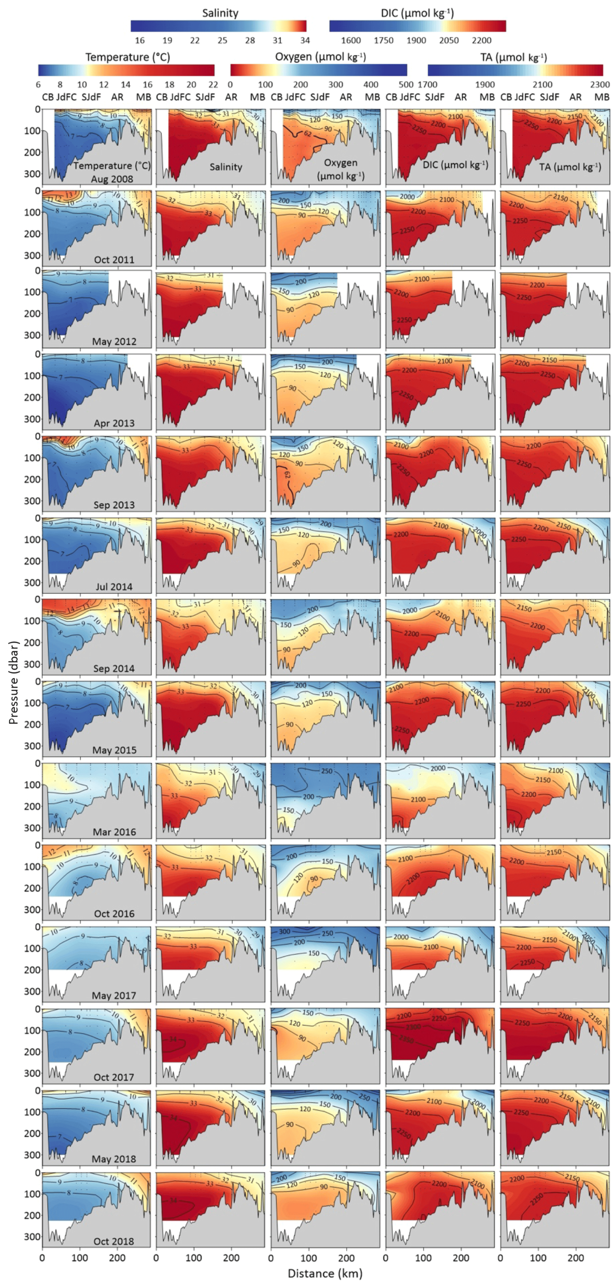
Figure 4 Depth-transect plots from Sound-to-Sea cruises for CTD temperature, salinity, adjusted CTD oxygen, dissolved inorganic carbon, and total alkalinity in the respective columns. The month and year when each cruise began is indicated in the left panel of each row. Each panel shows ocean conditions starting at the Ćhába⋅ mooring (CB), traveling through the Juan de Fuca Canyon (JdFC) and the Strait of Juan de Fuca (SJdF), over the glacial sills in Admiralty Reach (AR), and into the Main Basin (MB) of Puget Sound as the distance along transect increases (see map in Fig. 1). Color scales are the same for each parameter across Fig. 4 and the comparable Puget Sound figures (Figs. 5–9).

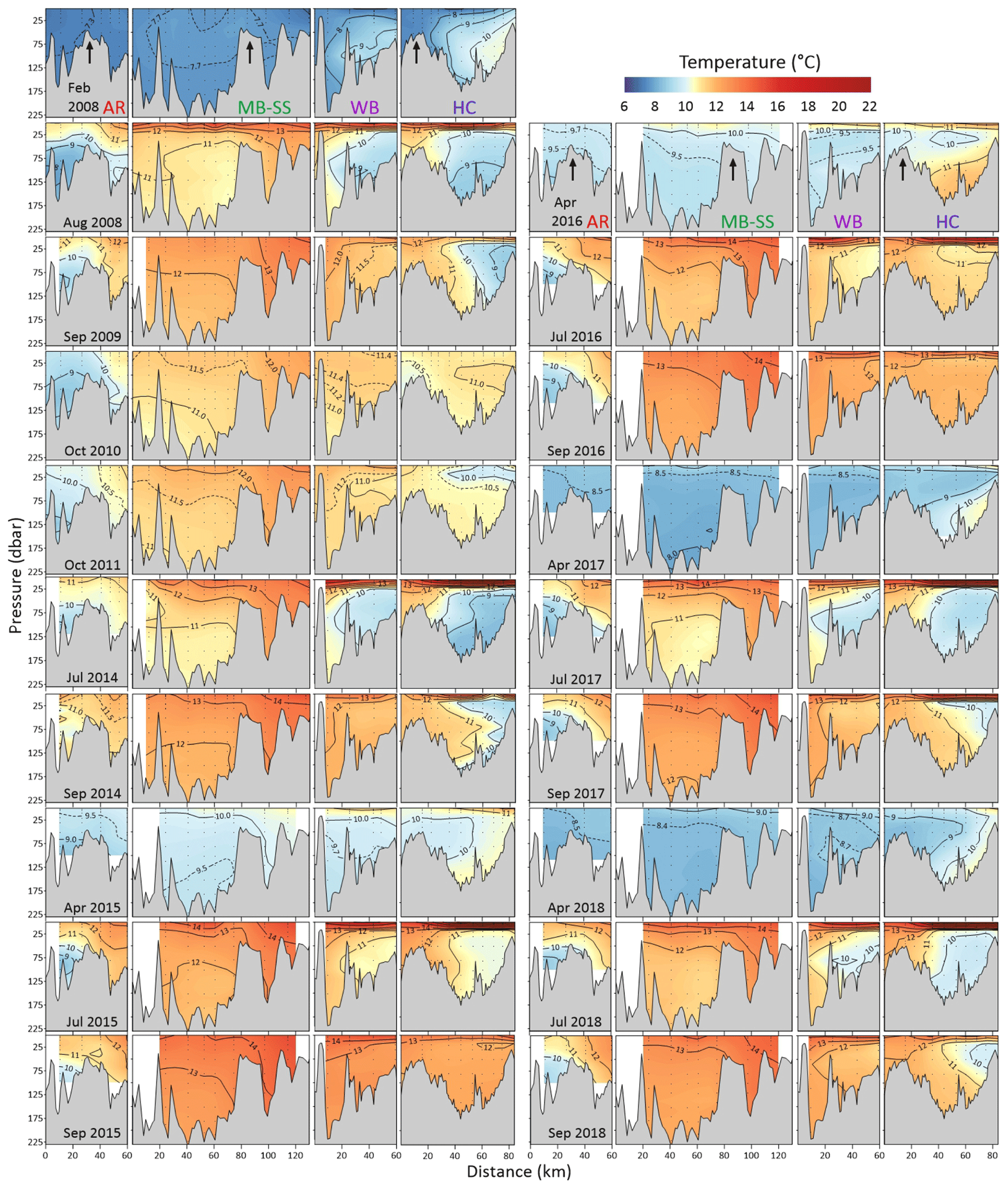
Figure 5 Depth-transect plots from all Puget Sound cruises by sub-basin for CTD temperature measurements, with the month and year when each cruise began indicated in the left panel of each row, noting that there are two columns consisting of four panels each to encompass all cruises. From left to right, panels within each column correspond to Admiralty Reach (AR), Main Basin–South Sound (MB–SS), Whidbey Basin (WB), and Hood Canal (HC). Colors of abbreviations correspond to station colors in Fig. 1. Admiralty Reach panels show the bathymetric profile and ocean conditions from the Strait of Juan de Fuca (SJdF) on the left going through Admiralty Reach toward Puget Sound on the right. The other three panels start at the nearest point on their respective transects inside Puget Sound from Admiralty Reach and progress to the distal end of the transects shown in the Fig. 1 inset map as distance along transect increases.

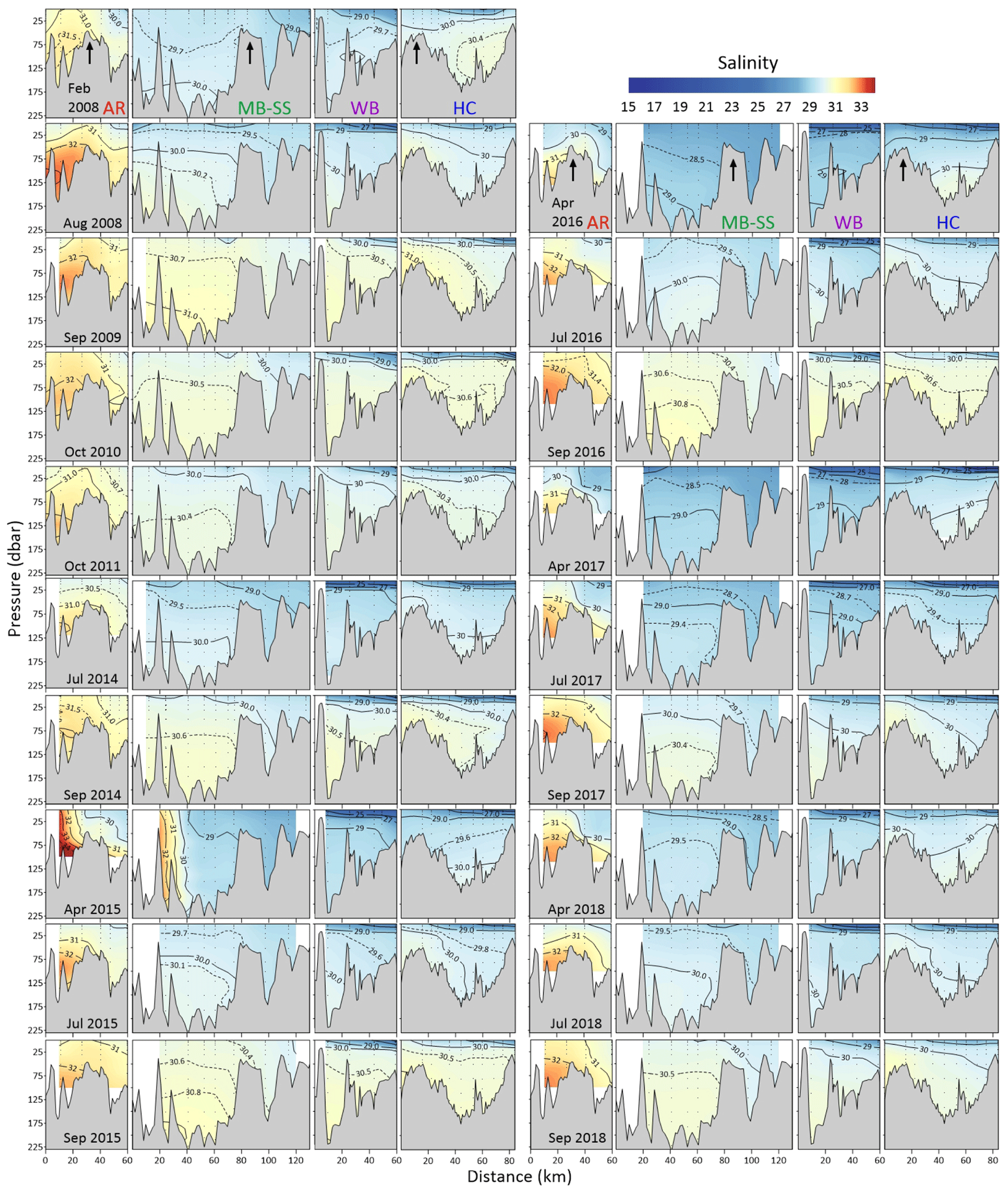
Figure 6 Depth-transect plots from all Puget Sound cruises for salinity. Figure organization is the same as in Fig. 5.

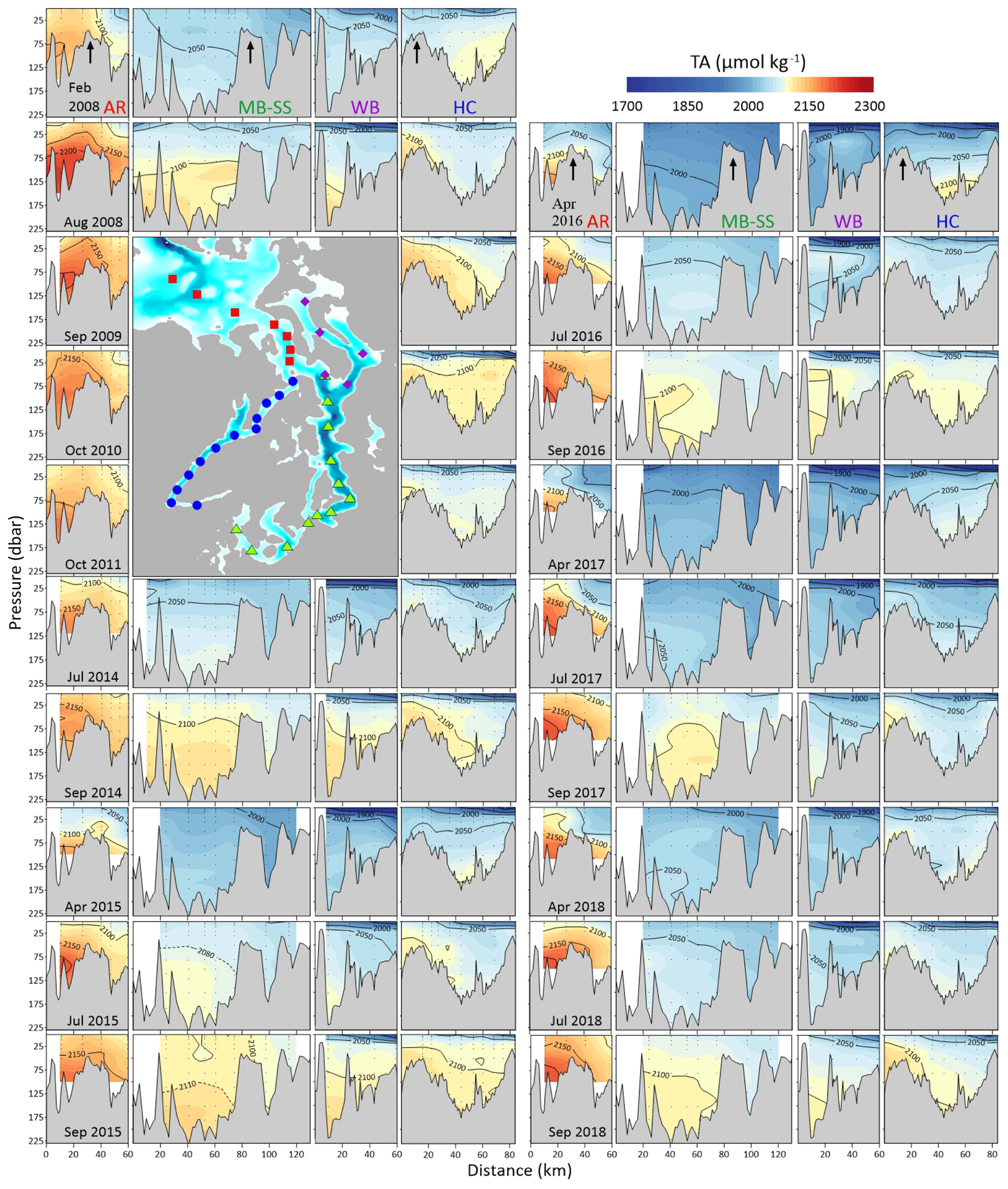
Figure 7 Depth-transect plots from all Puget Sound cruises for total alkalinity content (TA, µmol kg⁻¹). Figure organization is the same as in Fig. 5. The inset map shows sampling stations and is shown in place of data profiles for cruises that were not sampled for inorganic carbon parameters.

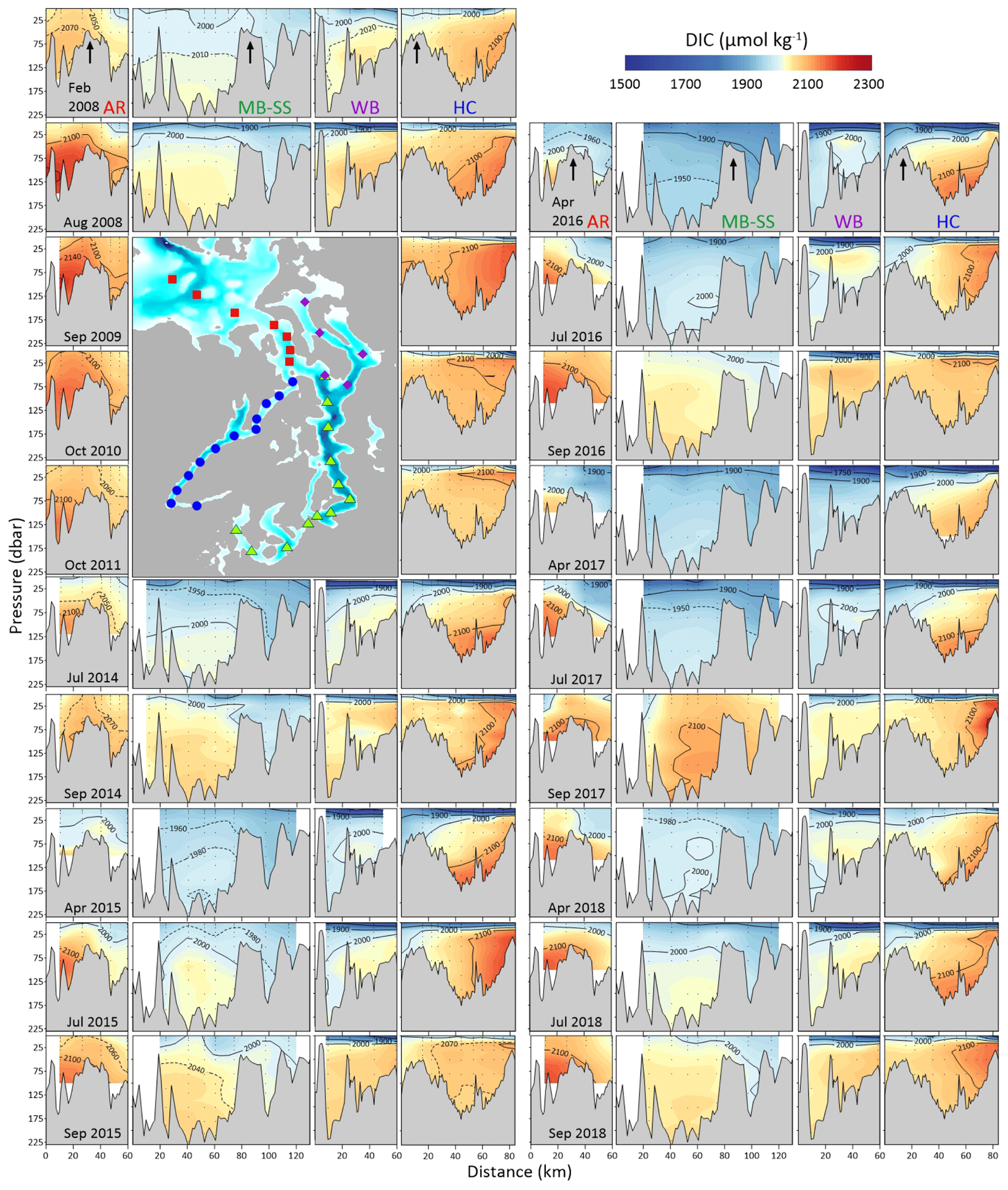
Figure 8 Depth-transect plots from all Puget Sound cruises for dissolved inorganic carbon content (DIC, µmol kg⁻¹). Figure organization is the same as in Fig. 5. The inset map shows sampling stations and is shown in place of data profiles for cruises that were not sampled for inorganic carbon parameters.

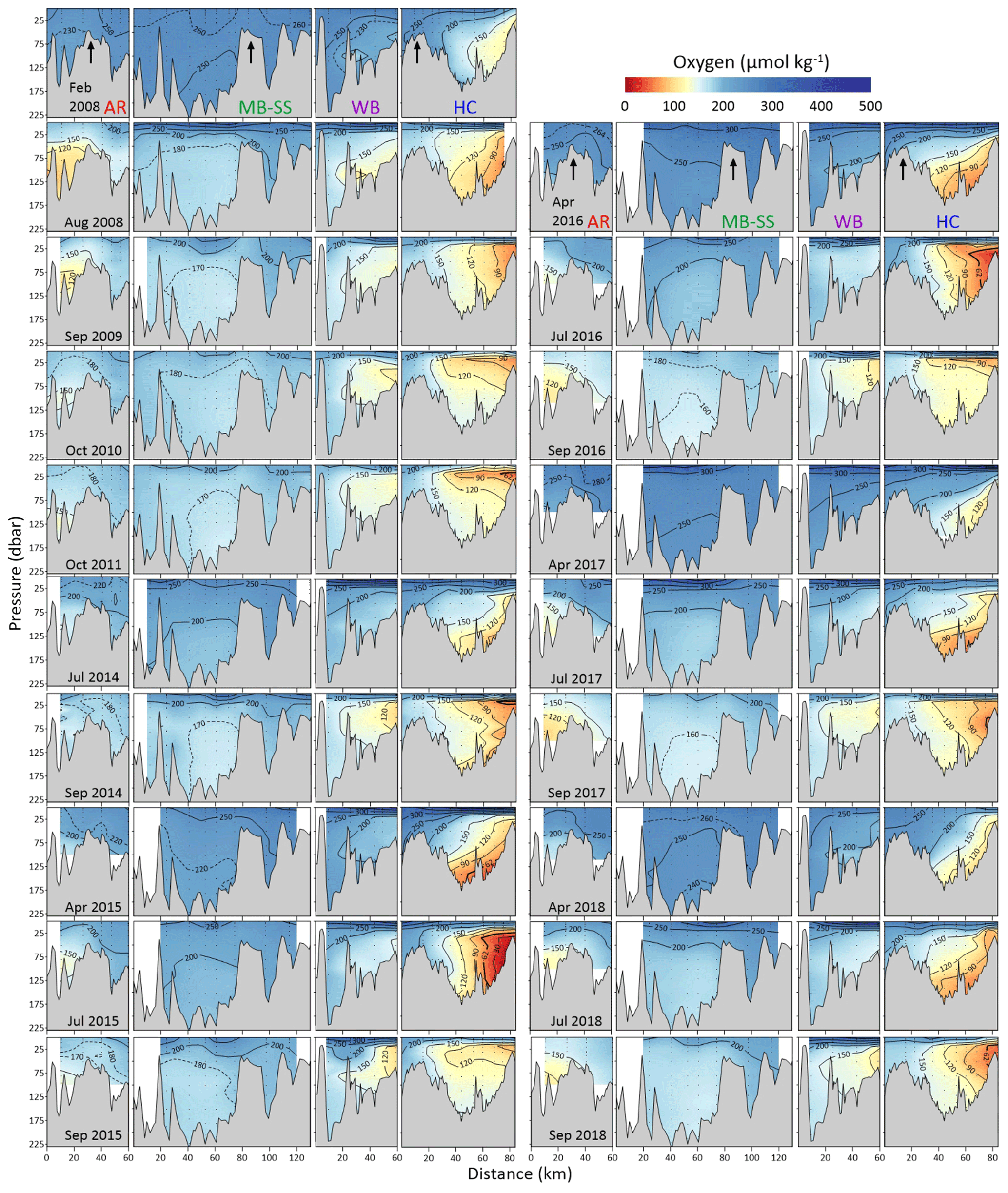
Figure 9 Depth-transect plots from all Puget Sound cruises for adjusted CTD oxygen content (O₂, µmol kg⁻¹). The bold contour at 62 µmol kg⁻¹ represents a commonly used hypoxia threshold. Figure organization is the same as in Fig. 5.

5 Applications and limitations of the Salish cruise data product

5.1 Using the Salish cruise time series to understand the ecological impacts of climate and ocean change

5.1.1 Past applications

A number of studies have already used Salish cruise data from this data product to describe variability in ocean conditions and provide context for understanding the physiological condition of and response to ocean acidification conditions for regionally important species, under both current and projected scenarios. For example, cruises included in this data product through 2014 were included in a large data compilation used to create seasonal climatologies for salinity, temperature, DIC, TA, and the calculated CO₂ system parameters CO₂ fugacity (fCO₂), pH (on the total scale), aragonite saturation state (Ω_arag), and Revelle factor (a buffering capacity metric), allowing end users to assess the range of average surface conditions expected in Washington's marine ecosystems (Fassbender et al., 2018). The same data compilation underpinned the development of an empirical TA–S relationship in Washington's marine surface waters (0–25 m) that allows users to estimate TA data using salinity as a proxy (Fassbender et al., 2017), providing end users a second surface carbon parameter for use in calculating the full CO₂ system and assessing acidification levels in ecosystems or stations with only a single carbon data stream. This approach could be especially useful for understanding conditions in nearshore ecosystems, where full constraint of the CO₂ system is often lacking (e.g., Jewett et al., 2020). Comparisons of observations further south in the California Current system have shown that upwelling water masses low in O₂ and high in CO₂ often influence nearshore ocean acidification and hypoxia (OAH) conditions (Chan et al., 2017; Kekuewa et al., 2022). However, freshwater influence is stronger in the northern California Current system and the Salish Sea, which can result in strong water column stratification and decoupling between shallow, nearshore, and deeper conditions offshore. The Salish cruise data product provides the opportunity to develop empirical relationships for more localized areas of the southern Salish Sea and its boundary waters, including deeper parts of the water column (e.g., Juranek et al., 2009; Alin et al., 2012), to provide more relevant biogeochemical context for local ecosystem monitoring than offshore observations can provide.

Observations at the spacing of discrete samples were used to generate the depth transects in Figs. 4–9. However, CTD cast data with a higher vertical resolution (0.5 dbar bins) can be used as a basis for interpolating conditions between the more widely spaced discrete measurements presented in this article. High-resolution downcast CTD data corresponding to all oceanographic profiles in this data product are also publicly available (http://www.nanoos.org, last access: 15 September 2023), but they were not analyzed or archived at the National Centers for Environmental Information (NCEI) with the Salish cruise data product. For example, Reum et al. (2014) created high-resolution depth profiles of temperature, O₂, pCO₂, and Ω_arag conditions across 2008–2011 Salish cruises at stations in Hood Canal and Admiralty Reach using partial least-squares regressions to interpolate conditions for each region and cruise. End users requiring higher-resolution water column information could use this interpolation approach based on combining the Salish cruise data product described here with downcast CTD data from the “Data” tab on the Northwest Association of Networked Ocean Observing Systems (NANOOS) Salish Cruise app (http://nvs.nanoos.org/CruiseSalish, last access: 15 September 2023), which provides the downcast, high-resolution complement of the CTD parameters described in this article using upcast data at discrete sample spacing. Files on the NANOOS app also include data for potential temperature, oxygen saturation (%), chlorophyll fluorescence, beam transmission, beam attenuation, potentiometric pH for some cruises (on the NBS pH scale), and photosynthetically active radiation.

5.1.2 Extended and potential future applications

The data product can also inform biological assessments. Many regional species have inferred or known sensitivity to ocean acidification parameters (pCO₂, partial pressure of CO₂; pH; and Ω) (Busch and McElhany, 2016; Jones et al., 2018). The early part of this time series was used to delineate the range of physical and biogeochemical conditions encountered by species of ecological or economic importance in the region (Reum et al., 2014, 2016). Pteropods, an exemplar of ocean acidification impacts, have been shown to experience pronounced dissolution in the Salish Sea, particularly in the more stratified and acidified basins (Bednaršek et al., 2021). Ongoing laboratory and field research to better understand the sensitivity of regionally important species (e.g., Miller et al., 2016; Bednaršek et al., 2020a, b, 2021, 2022; McElhany et al., 2022) has thus been able to use observed ranges and combinations of conditions encountered in the region for physical and OAH parameters rather than projections of future global ocean conditions that are often substantially inappropriate for representing the more dynamic and acidified conditions in coastal and estuarine ecosystems in Washington waters (Feely et al., 2008, 2016; Siedlecki et al., 2021).

An analysis of seasonal and interannual variability in the Salish cruise data product has provided preliminary information about the severity and relative frequency of ocean acidification, hypoxia, and marine heatwave conditions in the southern Salish Sea (Alin et al., 2023a). In combination with regional physical and oceanographic models (Khangaonkar et al., 2012; Siedlecki et al., 2016; MacCready et al., 2021), the Salish cruise data product can thus facilitate the extension of holistic vulnerability assessments like those that have been done for important shellfish fisheries on the coast (e.g., Hodgson et al., 2018; Berger et al., 2021) into Puget Sound, where the shellfish aquaculture industry contributed USD 184 million of economic activity, USD 77.1 million of labor income, and 2710 jobs to the Washington state economy in 2010 (Northern Economics, Inc., 2013). Past studies have examined the distribution of Dungeness crab populations in Hood Canal, which are the target of valued regional tribal and recreational harvests, in response to hypoxia levels along the basin (Froehlich et al., 2014). The Salish cruise data product may facilitate a deeper look at whether crab populations respond to chronically acidified conditions in a similar way (Alin et al., 2023a, b), based on known responses to elevated CO₂ and decreased Ω and pH conditions as well the biological responses during their critical life stages (Miller et al., 2016; Bednaršek et al., 2020a; McElhany et al., 2022). Finally, the Salish cruise data product can provide an important validation data set for the physical and biogeochemical parameters represented in the complex 3-D numerical simulations that contribute to vulnerability assessments. Appropriate regional models operate on timescales from daily to seasonal forecasts (e.g., Siedlecki et al., 2015, 2016; MacCready et al., 2021) to multiyear hindcasts (Khangaonkar et al., 2021) or end-of-century projections (Khangaonkar et al., 2019; Bednaršek et al., 2020b; Siedlecki et al., 2021).

The West Coast Ocean Data Portal is funding an effort to develop ocean indicators, including one to track the ocean acidification status across the entire US West Coast. Moored observations and numerical models allow the estimation of indicators such as the percentage of time or volume of water over which a location experiences conditions that surpass a given threshold (e.g., Sutton et al., 2016; Feely et al., 2024). Where estimates of preindustrial-era CO₂ system conditions are available, they can provide a means of gauging the magnitude of change due to anthropogenic CO₂ vs. natural processes or other anthropogenic causes (Sutton et al., 2016; Alin et al., 2023b). The Salish cruise data product offers the potential for creating seasonal OA indicators that estimate, e.g., the percentage of the water column occupied by conditions that exceed a biological threshold. Another OA indicator could be the expansion (in percent) of corrosive (Ω<1) water since the preindustrial era within the more inland basins of the southern Salish Sea. The development of such indicators would further expand the applicability of Salish cruise data to the management of natural resources and water quality.

5.2 Data product limitations

The compiled Salish cruise data product provides observations from 35 cruises, each with coverage of at least part of the study region and providing spatial and depth sampling coverage not afforded by other platforms in inland waters. However, the temporal resolution is at best seasonal, due to the expense and labor associated with conducting shipboard surveys. Thus, sampling of short-term events and illuminating the timeline of longer-lasting anomalies cannot be done solely with the Salish cruise data product. Fortunately, the region is also home to a number of time-series moorings that can be used to provide higher-resolution context for these detailed cruise observations at select locations through the study area (e.g., Northwest Environmental Moorings, https://nwem.apl.washington.edu/, last access: 15 September 2023; and Olympic Coast National Marine Sanctuaries oceanographic moorings, https://olympiccoast.noaa.gov/science/oceanographic-moorings/, last access: 15 September 2023). Multiple numerical models provide hindcasts and projections of ocean physical and biogeochemical conditions on daily to end-of-century timescales in the region as well. Using a combination of oceanographic observations and models, end users of this data product may be able to fill gaps in spatial or depth coverage to fulfill diverse research objectives.

6 Data availability

All finalized data described in this publication can be accessed through the Ocean Carbon and Acidification data portal on the NOAA National Centers for Environmental Information website (Alin et al., 2022; https://doi.org/10.25921/zgk5-ep63). After navigating to the HTTPS download link, the user can select one of the three data product versions described in Sect. 4.1 above. File name “SalishCruise_dataProduct_2008to2018_09202023_CO2calcs.csv” contains the smallest subset of the data product, consisting of 3971 complete records of DIC, TA, T, S, O₂, and nutrient measurements with the highest-quality QC flags, ready for calculations of the full carbonate system; this file is recommended for end users without strong familiarity with QC procedures or the interpolation of biogeochemical data. File name “SalishCruise_dataProduct_2008to2018_09202023_questNut.csv” contains an additional 50 samples with nutrient data that require further QC attention (total of 4021 paired observations); all other data have acceptable QC flags. File name “SalishCruise_dataProduct_2008to2018_09202023_allData.csv” contains the most complete version of the Salish cruise data product, including all data with questionable QC flags and data gaps for users with the capacity for or interest in interpolating to fill data gaps (total of 7525 records). An Excel file with updated metadata, including a tab detailing changes since the previous version of the data product on the NCEI page, is also available (“SalishCruise_dataProduct_2008to2018_metadata_09182023. xlsx”). The index of data product files for download can also be accessed via our NCEI landing page (https://www.ncei.noaa.gov/access/ocean-carbon-acidification-data-system/oceans/SalishCruise_DataPackage.html, last access: 18 September 2023), which shows the map available for download on the HTTPS download page. Should users wish to download individual cruise data files or the original versions of each cruise submitted to NCEI, these are available in Table 1 on this landing page. To access the compiled data products from the landing page, the user would click the “Database Files” link to reach the index of data and metadata files associated with this data product (the same page reached via the HTTPS link described above). The data product files, along with a metadata file, a list of updates in more recent versions, and a standalone version of the map on the landing page, can be downloaded by clicking on the relevant file name on the index web page. End users are encouraged to use one of the compiled data sets described above, as these contain all updates to QC flags, and to always download and use the most recent version of each file.

7 Conclusions

The Salish cruise data product provides a compiled data product including 35 cruise data sets that occupied stations in the southern Salish Sea and its boundary waters in the Strait of Juan de Fuca and nearby coastal waters obtained from 715 profiles of oceanographic data. This data product offers end users access to a decade of cruise time-series data with consistent formatting and both concentration and substance content units for commonly used parameters like oxygen and nutrients. Data from all cruises underwent added quality control measures, including extensive property–property plotting of biogeochemical and physical parameters, to identify and flag data points that may be anomalous. However, because the Salish Sea experienced a number of strong environmental anomalies during the 2008–2018 cruise time series comprising the data product, anomalous data identified in this way were mostly flagged questionable rather than bad to allow end users to determine whether these data are ultimately suitable for their analyses. The Salish cruise data product presents climate-quality biogeochemical and physical oceanographic data from a productive, complex estuarine system with several basins with distinct water mass characteristics and dynamics. Thus, the data product assembles rich information that can be used to validate 3-D models of ocean conditions, frame biological sensitivity studies, and help end users and decision-makers understand the range of conditions throughout the region and the dynamic interannual variability in ocean acidification and hypoxia here.