Mapping rangeland health indicators in eastern Africa from 2000 to 2022

Tracking environmental change is important to ensure efficient and sustainable natural resources management. Eastern Africa is dominated by arid and semi-arid rangeland systems, where extensive grazing of livestock represents the primary livelihood for most people. Despite several mapping efforts, eastern Africa lacks accurate and reliable high-resolution maps of rangeland health necessary for many management, policy, and research purposes. Earth observation data offer the opportunity to assess spatiotemporal dynamics in rangeland health conditions at much higher spatial and temporal coverage than conventional approaches, which rely on in situ methods, while also complementing their accuracy. Using machine learning classification and linear unmixing, we produced rangeland health indicators – Landsat-based time series from 2000 to 2022 at 30 m spatial resolution for mapping land cover classes (LCCs) and vegetation fractional cover (VFC; including photosynthetic vegetation, non-photosynthetic vegetation, and bare ground) – two important data assets for deriving metrics of rangeland health in eastern Africa. Due to the scarcity of in situ measurements in the large, remote, and highly heterogeneous landscape, an algorithm was developed to combine high-resolution WorldView-2 and WorldView-3 satellite imagery at < 2 m resolutions with a limited set of ground observations to generate reference labels across the study region using visual photo-interpretation. The LCC algorithm yielded an overall accuracy of 0.856 when comparing predictions to our validation dataset comprised of a mixture of in situ observations and visual photo-interpretation from high-resolution imagery, with a kappa of 0.832; the VFC returned a R²=0.795, p < 2.$\mathrm{2}\times {\mathrm{10}}^{-\mathrm{16}}$, and normalized root mean squared error (nRMSE) = 0.123 when comparing predicted bare-ground fractions to visual photo-interpreted high-resolution imagery. Our products represent the first multi-decadal Landsat-resolution dataset specifically designed for mapping and monitoring rangelands health in eastern Africa including Kenya, Ethiopia, and Somalia, covering a total area of 745 840 km². These data can be valuable to a wide range of development, humanitarian, and ecological conservation efforts and are available at https://doi.org/10.5281/zenodo.7106166 (Soto et al., 2023) and Google Earth Engine (GEE; details in the “Data availability” section).

1 Introduction

Rangelands cover nearly half of the African continent land mass and support the livelihoods of tens of millions of households (Reid et al., 2008; Sayre et al., 2013). The productivity of these rangelands along with the human and livestock populations they sustain is significantly affected by land degradation due to soil erosion, cropland expansion, and shrub encroachment resulting from heavy grazing and suppression of fires, as well as climate change (Barbier and Hochard, 2018; Roques et al., 2001; Angassa and Oba, 2008; Wynants et al., 2019; Vetter, 2005; Hoffman and Vogel, 2008). Episodes of extreme climate events, in particular, drought, have led to emergency population migrations and humanitarian crises of historic proportions (Blackwell, 2010). Improved understanding of the variation in rangeland health across space and over time is crucial for community development, ecological conservation, and humanitarian programming in the region.

The extensive development of Earth observation (EO) platforms has largely improved our understanding of ecosystems (Giuliani et al., 2020; Sudmanns et al., 2020). Long-term EO systems, such as the Landsat constellation, have provided valuable data to assess and accurately detect multiple ecosystem functions and patterns (Wulder et al., 2012; Loveland and Dwyer, 2012; Williams et al., 2006). Further development of EO and analytics has allowed the integration of multiple platforms into complex algorithms and workflows, benefiting from the ability of image data to scale at different spatial and temporal levels (e.g., AghaKouchak et al., 2015) and leading to paradigm shift from change detection to continuous monitoring at high resolution (Woodcock et al., 2022). These recent developments have led to much interest in applying EO and related analytics to rangeland ecology and management (e.g., Allred et al., 2021; Hill et al., 2020; Rigge et al., 2020; Fava and Vrieling, 2021).

Rangeland health has been conceptualized as a framework of three fundamental attributes reflecting soil/site stability, biotic integrity, and hydrologic function (Pellant et al., 2020). Historically, associated assessments have largely relied on in situ methods for assessment. Recent scientific advances create an opportunity to map rangeland health using satellite imagery to monitor changes at ecologically meaningful scales for landscape planning and management (Allred et al., 2022). EO in these often remote, arid and semi-arid regions becomes extremely valuable for its capacity to enable measurements in areas where data have never or rarely been collected on the ground. In addition, high-resolution (HR) remote sensing datasets can capture the fine spatial heterogeneity and the temporal dynamics that are key to informing management decisions but are also exceedingly difficult to discern at scale using conventional, ground-based monitoring systems (Zhou et al., 2020). EO-based data have been used to inform on rangeland health since the early days of EO programs (e.g., Landsat 1 program: Graetz et al., 1976). Understanding of rangeland ecosystems relies on information about the specific composition of the various vegetation communities within these ecosystems, oftentimes over large spatial extents, such as the Great Plains in North America (Reeves and Baggett, 2014). Composition changes over time are important to track trajectories, such as bush encroachment and soil degradation and impacts on grazers (Ghafari et al., 2018; Liao et al., 2018). HR thematic mapping of rangeland ecosystem can help explain key interannual variability in ecological processes such as water changes (Cooley et al., 2017), terrestrial and aquatic vegetation phenology (Cheng et al., 2020; Coffer et al., 2020), and crop dynamics (Lin et al., 2021), as well as long-term effects, such as land-use change, aboveground carbon, and sedimentation (Sankey et al., 2019, 2021).

The lower computational barriers from the continuous advancement of technology are promoting the shift from plot-based assessments to the integration of satellite-based maps into landscape management, improving broad-scale mapping of rangelands at higher spatial and temporal resolutions than ever before (Jones et al., 2020; Allred et al., 2022). Many recent contributions to this field have shown that even though moderate resolution datasets (from MODIS sensors at 250 m resolution) are able to detect short-term vegetation phenology and long-term demographic dynamics of herbaceous and woody species, they cannot detect changes at local scales because the spatial patterns of herbaceous and woody species typically occur at such fine scales (Angassa, 2014; Browning et al., 2017, 2019; Matongera et al., 2021; Oba et al., 2003). Despite collecting data at lower temporal resolutions, the Landsat collection at 30 m spatial resolution has consistently played an important role in science for over 50 years due to continuous efforts in calibration and corrections (Wulder et al., 2012, 2022; Franks et al., 2020). The recent collection-based reprocessing that resulted in the Landsat collection 2 (Wulder et al., 2022) represents an important opportunity to build consistent time series for rangeland mapping at local scales. In addition, field studies have demonstrated that Landsat-scale sub-pixel estimation of fractional cover of rangeland functional types, such as herbaceous and shrub components, and especially bare ground, is crucial to overcome the difficulties of parsing out the underlying heterogeneity within thematic land cover classifications and in understanding ecological dynamics (Jones et al., 2018; Rigge et al., 2019). As a result, land cover classification (LCC) and vegetation fractional cover (VFC; including photosynthetic vegetation (PV), non-photosynthetic vegetation (NPV), and bare ground (BG)) estimations have become the two building blocks of rangeland health assessment of today's EO-based rangeland management (Jones et al., 2020). However, Landsat-based land and fractional cover mapping over large and remote regions is hampered by the difficulty of collecting ground truth data at fine resolution. This is especially true in eastern Africa, where limited infrastructure and physical insecurity make it very difficult to collect field data at scale.

In this study, we produced a unique and new dataset composed of Landsat-based LCC and VFC annual estimates of rangeland components for eastern Africa from 2000 to 2022. We used a LCC scheme to help identify rangeland vegetation transition pathways and VFC to describe rangeland health condition trajectories within each class. To overcome the challenge of scarce ground data for training and validating our models over this vast and remote region, we used a large collection of high-resolution satellite imagery, visual photo-interpretation, and ad hoc algorithms to generate a large sample of reference data to generate and validate our two products.

2 Data and methods

The overall strategy of our methodological framework to generate the long-term time series of LCC and VFC for rangelands in eastern Africa consists of three major steps: first, the development of a training/testing dataset from HR imagery (Sect. 2.3); second, the LCC classification (Sect. 2.4); and third, the VFC classification (Sect. 2.5). The detailed workflow is provided in Fig. 1.

To integrate in situ and HR data to create reference data, we used ground reference data to inform a visual photo-interpretation (VPI) protocol to create reference labels to train supervised classifications of HR imagery. These HR classifications were used to create a large amount of machine-generated reference data to train Landsat-based classifiers and to identify areas with large proportions of the focal rangeland components for VFC estimation. To generate the LCC reference data, we generated an algorithm that created reference points using a set of conditions with the proportions of reference compositional component (RCC). The RCCs within each of our LCC definitions include vegetation functional groups (VFG) and other important classes such as bare ground. The RCCs are then compared to the calculated proportion of pixels from the HR classification within a moving window matching the 30 m spatial resolution of the Landsat data. We also generated VFC reference data using image segmentation on the RCC classifications with the assistance of an application in GEE to identify homogeneous areas of rangeland components that could spatially allocate Landsat pixels to use them to calculate spectral endmembers and generate VFC estimations. Figure 1 shows our general workflow, including reference data partitions, remote sensing data and results, processing algorithms, and accuracy assessments.

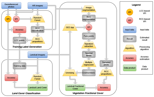
Figure 1 Schematic workflow of the process used in this work to generate land cover classifications and fractional cover estimations based on Landsat imagery. Short names correspond to the following: visual photo-interpretation (VPI), points generated with reference compositional component (RCC) work to train the RCC classification (RCC points); collection of points with pure pixels (i.e., points with 100 % of a single VFC type, pure points); library of spectral signatures of pure points (spectral library); spectral endmembers for PV, NPV, and BG (endmembers); random sample of points with overlapping Landsat imagery to perform accuracy assessment on VFC estimations (sampled pixels). See text for further details on the uses of data and processing.

Prior to the detailed technical description of this entire workflow (Sect. 2.4–2.6), we first described our study domain (Sect. 2.1) and satellite datasets utilized in this study (Sect. 2.2).

2.1 Study area

The study area is located in the semi-arid and arid regions centered in east and northern Kenya, western Somalia, and southern Ethiopia (Fig. 2). We chose this study region because it has been a geographic area with numerous development interventions on the ground in the past decades (Liao and Fei, 2017), but limited land cover datasets exist to evaluate the concurrent changes on the landscapes. In addition, this region suffers strongly from climate change extremes (e.g., droughts, floods; IPCC, 2022) and their consequences on rangeland health, resilience, and well-being of pastoralists (Pricope et al., 2013; Beal et al., 2023). Covering a total of 745 840 km², it includes diverse types of rangelands, which represent hyper complex and rapid physiological and phenological dynamics in other regions of the world (ILRI, IUCN, FAO, UNEP and ILC, 2021; Adams et al., 2021; Nandintsetseg et al., 2024). Therefore, the study area demonstrates potential for broad generalization and sheds light for development efforts for stakeholders.

We used two main features to bound our study area. To the east and north, we used Landsat tiles, using PATH 164 and ROW 56 as limits, dropping tiles PATH 164, ROW 59 and 60 due to heavy cloud cover. To the west and south, we used a threshold value of mean annual precipitation of 700 mm using TerraClimate data (smoothed with a kernel convolution with standard deviation = 5 km; Abatzoglou et al., 2018), thus keeping the focus on the rangeland-dominated arid and semi-arid areas.

The study covers the epoch 2000 to 2022 to help capture decadal variation in ecosystem conditions and maximize Landsat data availability. Landsat imagery is limited in this area due to high cloud cover often occurring during the two wet seasons observed in the region including the long rains (March to June) and short rains (October to December). In most cases, cloud-free data were available during December through early March, which corresponds to the short, dry (SD) season. Thus, we generated our datasets using imagery from a portion of the SD, from 15 December over 2000–2022 to 1 March over 2001–2023, which maximized the annual available data count per pixel and ensured even distribution of data over our period of study.

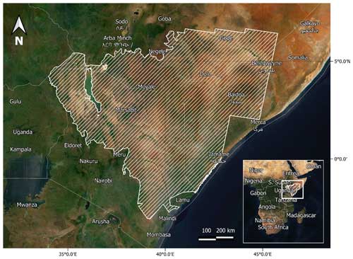
Figure 2 Map showing our study area in eastern Africa. Basemap: © MapTiler, https://www.maptiler.com/copyright/ (last access: 10 November 2023).

2.2 Remote sensing data

2.2.1 HR – high-resolution satellite imagery

To train our models and validate the results, we used HR satellite imagery as little ground reference information exists in this vast and remote region. We obtained a large collection of imagery from Maxar Technologies via the United States National Geospatial-Intelligence Agency (NGA): ordered with the following filtering parameters: sun elevation > 45°, off-nadir angle < 40°, and cloud cover < 50 %. The HR collection was composed of 2500 mosaicked strips of imagery scenes from Worldview-2 and Worldview-3 sensors (Fig. 3). These mosaicked strips, typically 16.4 km in width, were delivered as orthorectified and radiometrically corrected bundles of eight bands including coastal (400–450 nm), blue (450–510 nm), green (510–580 nm), yellow (585–625 nm), red (630–690 nm), red edge (705–745 nm), near-infrared 1 (NIR1, 770–895 nm), and NIR2 (860–1040 nm) at a spatial resolution of 184 cm for WorldView-2 and 124 cm for WorldView-3 and a panchromatic band at a spatial resolution of 46 cm for WorldView-2 and 31 cm for WorldView-3. Shortwave infrared (SWIR) imagery (1195 to 2365 nm) collected by Worldview-3 with a spatial resolution of ∼ 3.7 m was also used in this study.

After subsetting to the short, dry season, we manually selected 321 strips maximizing the spatial coverage and minimizing cloud cover, as most images with scattered clouds projected oblique shadows often resulting in < 10 % of pixels being usable for further analysis. These data corresponded to imagery acquired from 2016 to 2020. We considered using Quick Bird imagery from previous years, but data availability for our area of interest was minimal.

Figure 3 Spatial coverage of high-resolution imagery (polygons) and the spatial distribution of the point grid (dots) used for generating reference data.

2.2.2 Landsat collections

To capture historical changes in vegetation health in our area of study, we utilized the Landsat dataset, which has been available for over 4 decades (1982–present; Wulder et al., 2012) and thus enables the development of long-term time series of land cover classes and vegetation fractional cover. While other studies have shown the value of higher-resolution sensors such as Sentinel-2 to show the potential higher gain in accuracy compared to Landsat collection for the detection of invasive species in eastern Africa (Dube et al., 2020), ESA's Sentinel mission only features a short history of imagery acquisition from 2015 (Drusch et al., 2012), which could bias our assessment towards the last decade, thus confusing the interpretation of our results.

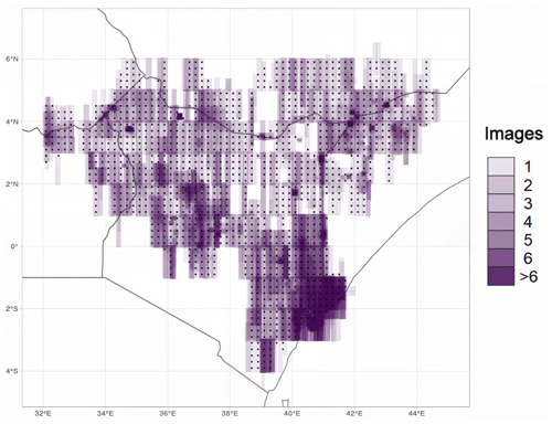
Landsat data are readily and freely accessible for scientific purposes. They are available at different processing levels, from raw images to radiometrically, geometrically, and atmospherically corrected scenes (Wulder et al., 2019). We used Google Earth Engine (GEE; Gorelick et al., 2017) to access and analyze atmospherically corrected surface reflectance images for Landsat 5, 7, and 8 satellites from collection 2 (USGS, 2021), processed at the L1TP level (https://www.usgs.gov/core-science-systems/nli/landsat/landsat-levels-processing, last access: 10 November 2023). Landsat data are packaged into overlapping “tiles”, covering approximately 170×183 km each, using a standardized reference grid (USGS, 2019). In this study we used 42 of these tiles, totaling 1 192 654 km² (Fig. 4). Differences in Landsat satellite sensors require different processing and correction techniques. We describe each sensor first and then outline our harmonization efforts.

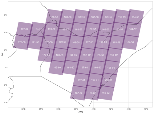
Figure 4 Spatial coverage of Landsat tiles used in this study spanning from 2000–2022. Numbers within each tile correspond to the PATH and ROW used in the storage protocol for Landsat data.

The Landsat 8 Operational Land Imager (OLI) uses data comprised of five visible and near-infrared bands: coastal aerosol, blue, green, red, and infrared (NIR) and two shortwave infrared (SWIR1 and 2). All bands were atmospherically corrected using the LaSRC (Land Surface Reflectance Code; USGS, 2019). Other auxiliary data includes cloud, shadow, water, and snow mask layers generated with the C Function of Mask (CFMask) algorithm version 3.3.1 and stored in the Pixel Quality Assessment Band (QA_PIXEL; Foga et al., 2017; USGS, 2022), as well as a saturation mask band in the Radiometric Saturation Quality Assessment Band (QA_RADSAT).

Landsat 5 (TM) and 7 Enhanced Thematic Mapper Plus (ETM+) data also contain different types of observation bands according to their position in the electromagnetic spectrum. In the visible, near-infrared, and SWIR bands, blue, green, red, infrared (NIR), and SWIR1 and SWIR2 bands are processed to convert raw values to orthorectified surface reflectance values. All bands have a resolution of 30 m per pixel. All bands were atmospherically corrected using LEDAPS (Schmidt et al., 2013). Other auxiliary data include cloud, shadow, water, and snow mask layers generated with the CFMask algorithm and stored in the QA_PIXEL band, as well as a saturation mask band in the QA_RADSAT band.

Landsat 7 has the potential to help fill the gaps between Landsat 5 and 8, being available from the year 1999 to date. However, the failure of the Scan Line Corrector (SLC) of Landsat 7 in 2003 somewhat limits its utility (Markham et al., 2004). This failure resulted in areas that are not imaged (∼ 22 % of each tile); otherwise, data are valid for work and analysis. These data show similar distribution of cloud cover and revisiting times as Landsat 8 collection. Hereafter, we refer to data pixels as any pixel where no masking occurred, and valid and usable data were available.

2.2.3 Landsat collection harmonization

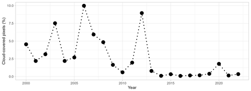
We used reduced major axis regression to harmonize the surface reflectance values from Landsat 5 and 7 to match the spectral information of Landsat 8 following Roy et al. (2016) on each Landsat data tile. These transformations are performed to improve temporal continuity between Landsat sensors (TM, ETM+, and OLI). After harmonization, the collections were merged and annual composites from 15 December to 1 March were generated using the median value of available data pixels. We used the median value as the mean often gets biased with cloud contaminated pixels that were not included in the Level-1 QA_PIXEL band used for cloud masking. In this study, the year of the annual composites corresponds to the calendar year where the composite starts (i.e., 15 December). We selected this time interval as it was when imagery was mostly available, thus minimizing temporal imbalances among annual estimations. However, a large proportion of pixels were masked as a result of heavy cloud cover, with more than 5 % of masked pixels in 4 out of 21 different years. The year 2006 was a particularly problematic year, where the cloud component resulted in 10 % of pixels being masked (Fig. 5). The launch of Landsat 8 in 2013 not only implied an improvement in the sensor characteristics, but also increased data collection capacity, thus reducing the likelihood of acquiring cloud-covered imagery as is evident in our study area (Fig. 5).

Figure 5 Cloud-covered pixels present in the short, dry (SD) season composites of Landsat imagery used in this study.

2.3 Development of training/testing datasets by integration of in situ and HR data

2.3.1 VPI – reference dataset by visual photo-interpretation of HR imagery

We applied this classification scheme using VPI methods to develop training data for the classification algorithms for both LCC and VFC. We started first at the Borana Zone in southern Ethiopia, in the northern portion of our area of interest (AOI) where a rich source of georeferenced, ground-based photography (N = 1419 photos) was available for both a dry season (28 June–26 August 2013) and a wet season (6–31 May 2014; Liao et al., 2018). In this VPI work, we leveraged this photography with HR satellite imagery of the same locations and approximate time frames to capitalize on the differing contextual strengths of each data source. The photography provided a low-angle oblique view of vegetation functional groups and canopy layers for better class identification. The HR imagery, viewed via Google Earth (GE) or via United States National Geospatial-intelligence Agency's (NGA) Global Enhanced GEOINT Delivery (G-EGD), provided a broader, nadir-oriented view of differing vegetation stands in context with one another, allowing more confident class separation.

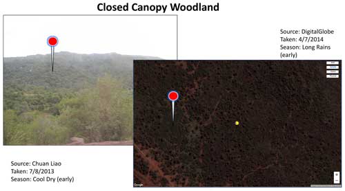
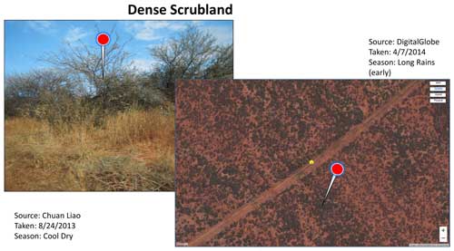
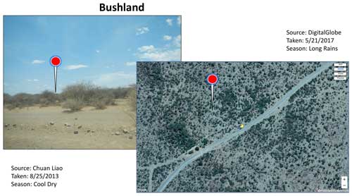
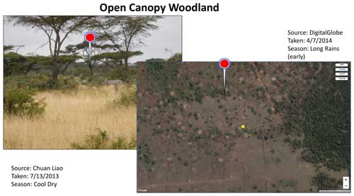
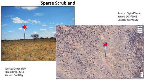
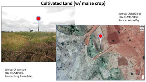
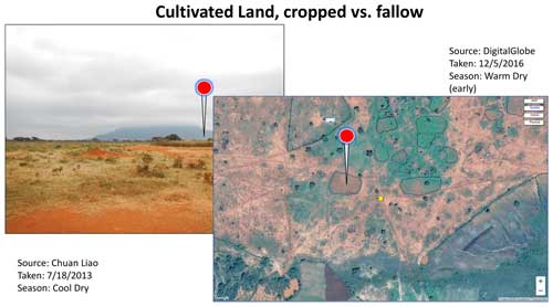
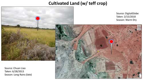
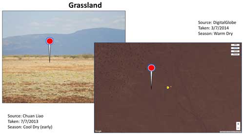
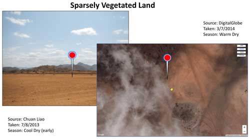
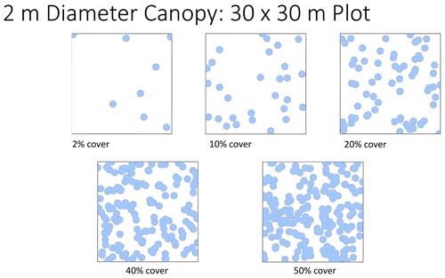
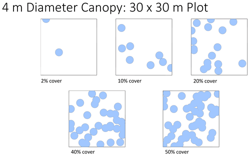
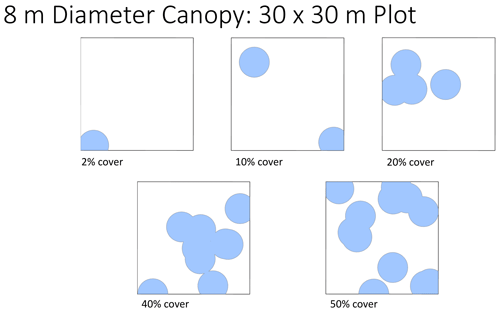
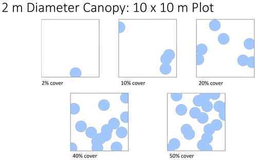
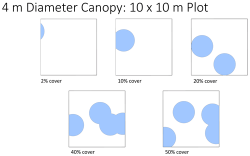
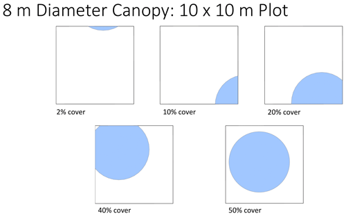
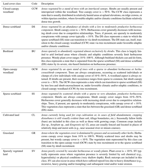
Specifically, a team of four VPI analysts was trained to identify eight land cover classes following those employed by Liao and Clark (2018). We made additional refinements to these classes as detailed in Table 1. A detailed protocol was developed to ensure effective quality control. Training materials included reference flash card sets (see Appendix B) created for each of our land cover classes depicting a ground-based oblique view of a stand of representative vegetation in addition to a nadir HR satellite view of that same stand in context with other surrounding vegetation in the locale. Canopy cover flash card sets were also created for 2, 4, and 8 m shrub and tree crown diameters to aid in visually estimating cover percentages relative to the thresholds separating each land cover class. The VPI classification was calibrated using the reference card sets and a standardized set of VPI points and associated photographs and imagery. Upon implementation, periodic spot checks of each analyst's VPI classifications were conducted to affirm consistency and accuracy.

Table 1 Land cover classes used for the Landsat land cover mapping (modified from Liao and Clark, 2018).

VPI classification took place as follows. The VPI point set from the georeferenced photograph locations was randomly subset into equal partitions, and each partition was assigned to a VPI analyst. The software package Nikon ViewNXi™ was used to view the photographs and mapped camera location and oblique view direction on a satellite imagery background provided by the software. The camera location coordinates were then plotted in GE, and vegetation at the location was evaluated using HR imagery that was concurrent or nearly concurrent with that of the photograph. Where concurrent imagery was missing from GE, imagery from the NGA archive was ordered and viewed via G-EGD, and a VPI-based classification was made for the camera location. Where the camera location occurred in a mixed or ecotonal area, a new point in a nearby, more representative location (i.e., more homogenous vegetation structure, cover, and composition) was selected by the analyst and classified in a land cover class. Upon completion of the VPI classification, a random sample of 10 % of the 1419 VPI points was spot-checked to confirm overall consistency and accuracy across analysts. Where consistent bias or misclassification was found, additional training was provided, and the analyst(s) re-visited all assigned points for the troublesome class or classes and re-classified these points as necessary.

As the extent of this dataset was limited to the north area of our AOI, we extended the use of this dataset as reference to inform recognition of the vegetation functional group components of each land cover class used here. Vegetation functional groups generally refer to different types of vegetation that are functionally and structurally different. In our setting, the primary groups are trees, shrubs, and grasses. Using pan-sharpened HR imagery, we then performed independent VPI classifications of VFGs within classes to develop and refine a supervised machine classifier and to support fractional cover analyses which are described in the next sections. This additional VPI work followed a procedure to spatially label the key components within each of the land cover classes and was focused on a grid of 8×8 km squares centered in a regular point pattern where HR imagery was available (see Fig. 3). These reference compositional components (RCCs) included the vegetation functional groups (trees, shrubs, grass) as well as bare ground, water, cultivated land, and impervious surfaces. We leveraged the combination of nadir views from HR satellite imagery and the large set of available landscape photographs from the northern portions of our AOI to recognize visible characteristics of each sub-class component and apply these characteristics in VPI classification of the entire study area.

2.3.2 RCC – reference compositional component classification of HR imagery

To create the reference dataset for calibration and validation of LCC and VFC estimations for our entire study area, we relied on RCC data generated from the classification of HR imagery. RCCs represent the basis of LCC as our land cover scheme (see below) follows a compositional combination of them. In addition, RCCs are an important input for VFC estimation, which needs to be complemented with non-photosynthetic vegetation reference points, created with a different approach (see below).

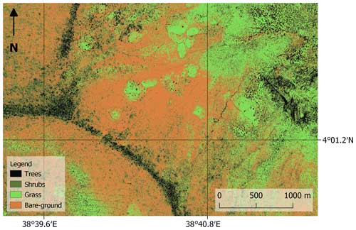
We calculated the normalized difference vegetation index (NDVI) from the red and NIR-1 bands of the HR imagery and then added the NDVI as a new band to the HR dataset. Spectral signals were then extracted and assigned to the points generated in the HR VPI work with each assigned RCC class, and a random forest classification was performed to predict RCCs using the spectral information as covariates. The number of trees was set to 1000, with two variables tried at each split. After model fitting, we used a graph showing the out-of-bag error of each class versus the number of trees in the classification to explore the effects of sample sizes on the accuracy of the method and increase it when needed. Classification of HR imagery focused on classifying RCCs – trees, shrubs, grasses, bare ground, water, cultivated land, and impervious surfaces (e.g., Fig. 6). After training our classification algorithms on 90 % of the generated labels, we then used the remaining 10 % to compare the (out-of-sample, OOS) prediction of the classifier against the actual reference labels using confusion matrices. We set a threshold minimum value of 85 % overall accuracy for using the resulting classifications in the following analysis steps. A random sample of HR classified imagery with accuracies above the threshold was selected and visually inspected to understand misclassifications and their potential drivers. We increased our RCC-oriented VPI effort if threshold levels were not met until accuracy met our threshold value. Despite our efforts and due to cloud cover and other factors such as cropland misclassifications in humid areas, only 44.5 % (n = 143) of the total RCC classifications were retained using the 85 % accuracy threshold. Lower-accuracy classifications occurred in areas of highlands on the west and southeast portions of our study area, characterized by higher precipitation. After contrasting classification predictions against pan-sharpened images, we recognized that most of the misclassifications corresponded to classes including green vegetation such as grass, crops, and trees. Other sources of error included areas with cloud shadows and impervious surfaces.

Figure 6 Example of a RCC classification result using a Worldview-3 image.

2.3.3 Composition-based algorithm for HR reference data creation

After classifying HR strips and selecting those with higher accuracy, we applied a custom-made algorithm that uses a squared moving window of the size of a Landsat pixel (30×30 m) and calculates the proportion of HR pixels, representing the area in the window covered by each of the RCC classes from the predicted HR classification. Using the proportion of HR pixels for each RCC class allowed us to use both Worldview datasets, as they have different spatial resolution. Then, using the list of defined threshold compositional percentages of RCC classes per land cover class in Table 1, we built code to meet the criteria for each land cover class. We then selected a stratified random sample of 80 000 points to be used as training points for the Landsat classification, described next. Points retained the date of the HR strip used to generate them. Due to misclassifications associated with scattered cloud cover in some imagery, we further applied a buffer of 500 m around areas where more than 100 pixels of cloud or shadows were detected inside the moving window described above and excluded these from the RCC proportion calculation and class assignment.

2.4 Land cover classification

2.4.1 Land cover classification model

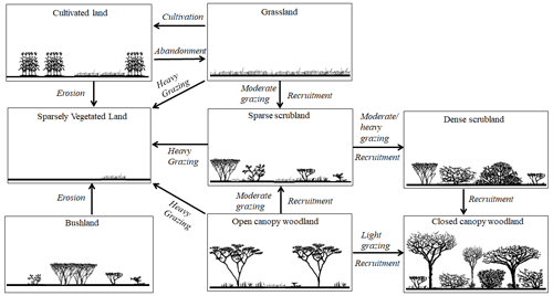
Our LCC scheme is based on the state-and-transition model (STM; Bestelmeyer et al., 2017; Steele et al., 2012; Blanco et al., 2014) developed for this region by Liao and Clark (2018), with adjustments based on contributions from Pratt et al. (1966) and Liao et al. (2018) (Fig. 7). Specific changes included the addition of classes not included in Liao and Clark (2018) and more precise definitions of the characteristics of each class and the trajectories between them, given the extension of our study area. The scheme includes eight land cover classes, each representing a vegetation state defined by structure, cover, and functional group composition. The potential transitions among these states or classes are described in the mapping legend provided in Table 1, which adapts Table 1 from Liao and Clark (2018). However, tree, shrub, and herbaceous cover thresholds have been further refined to better define class separations. The bushland class was also more clearly defined as a state where herbaceous presence was severely limited by climatic and/or edaphic factors rather than interspecific competition with shrubs and/or trees for resources. Transition pathways associated with wild or prescribed fires have been excluded from Fig. 7 and the legend (Table 1) to simplify description and presentation given the complexities associated with fire-tolerant versus fire-intolerant woody species, wildfire control, and past prohibitions on prescribed fire.

Figure 7 States and transition pathways among eight land cover classes.

2.4.2 Land cover classification algorithm

The land cover classification consists of two general steps. First, the HR imagery was classified using the combination of RCC labels generated from VPI work (described in Sect. 2.3.2) and random forest classifiers (Belgiu and Drăguţ, 2016), producing RCC classifications. Second, an automatic algorithm, based on conditionals and the percentage thresholds of RCC defining each LCC (described in Table 1), was run over the RCC classifications to generate new training labels for the classification of the Landsat collections with a second random forest classifier. Here, we describe the Landsat classifications.

Landsat collections were classified using the random points generated from the RCC classifications (see Sect. 2.3.3). We reserved 1419 in situ points from Liao and Clark (2018), so we could later use this dataset with HR ground reference data to independently assess the accuracy of our results. We first masked all Landsat images using the SR_CLOUD_QA band generated from the CFMASK algorithm of Landsat Surface Reflectance data. To eliminate water bodies and rivers in our AOI, we applied a normalized difference water index (NDWI) mask, whereby pixels with values > 0.2 were removed (Gao, 1996). We also calculated and added enhanced vegetation index (EVI), modified soil adjusted vegetation index 2 (MSAVI2), and normalized difference water index (NDWI) bands to the collections (Qi et al., 1994; Liu and Huete., 1995; McFeeters, 1996). We also used CGIAR SRTM 90 m Digital Elevation Database version 4 to include elevation and derived slope and horizontal curvature (Jarvis et al., 2008; Safanelli et al., 2020). Last, we included the bare-ground and photosynthetic vegetation fractions from our fractional cover results (see Fig. 1) as covariates, which were found to increase accuracy during our testing/tuning stage. We used the 80 000 algorithm-generated training points through the RCC classification protocol explained in Sect. 2.3 and randomly partitioned them into 90 % training and 10 % for accuracy assessment. We then extracted the spectral information from the Landsat composite corresponding to the year of the date of each HR image used to generate the training points through VPI work (see Sect. 2.3.1). With these points, we trained a random forest algorithm to predict the vegetation classes of the entire collection. Thus, a single multi-year random forest classifier was used for prediction on the harmonized Landsat collection. After initial tuning of the classifier, we used 20 trees and a maximum number of 50 nodes. The resulting classified collection includes images with pixel values associated with our main land cover classes and masked pixels of cloud cover, shadows, and water.

2.4.3 Accuracy assessment of land cover classification

We used multiple reference year calibration to generate a classification model dependent on the surface reflectance data (Gómez et al., 2016). Based on the standard assumption that surface reflectance data represent the true ground response of features to sunlight, the classification model is then used to predict past and future time steps in the remote sensing time series. Often, these data are referred to as absolute-normalized data (radiometrically and atmospherically corrected and orthorectified; Thenkabail, 2015). After generating reference labels through the combination of HR imagery classification and an area-proportional classifier to upscale VFGs to land cover classes, we randomly partitioned this reference dataset into training (90 %) and validation (10 %). We used the validation partition with the addition of the 1419 points from Liao and Clark (2018) to create confusion matrices to assess the accuracy of the predictions. The percentage of classes in the random validation sample relative to the total amount of reference data was 9.3 % for CCW, 14.5 % for DS, 13.6 % for BU, 7.7 % for OCW, 9.6 % for SS, 1.7 % for CL, 8.8 % for GR, and 16.7 % for SV (see Table 1 for class names).

2.5 Fractional cover classification

We used bilinear unmixing to estimate fractional cover (Quintano et al., 2012) of three components of rangeland: bare ground (BG), photosynthetic vegetation (PV), and non-photosynthetic vegetation (NPV). We combined HR and Landsat imagery to identify homogeneous areas where the spatial footprint of Landsat pixels could capture pure spectral signals for the three components of fractional cover. In this context, pure refers to pixels with 100 % cover of one of our three main components (Roberts et al., 1998). Given the heterogeneity of soil types in our study area, we allocated special effort on finding as many BG pixels as possible. To find these, we used the resulting RCC classification of HR imagery (see Sect. 2.2.2) and performed image segmentation to identify homogeneous areas covered by bare ground. Because Landsat pixels are 30 by 30 m and their footprints could change with each revisit, we built an algorithm to scan the classifications to find homogeneous areas larger than 50 by 50 m, in order to allocate Landsat pixels with a margin of 10 m in both spatial axes.

We used GEE to manually create a sample of pure pixels, by mapping different Landsat color composites and creating graphs of 10-year-long NDVI and MSAVI2 time series and spectral profiles (i.e., spectral signatures) including all bands from the Landsat imagery for visually selected locations in the map. Using these visualizations, we checked that Landsat pixels corresponding to BG always covered the extent of the focal area and were not contaminated by vegetation or other features such as litter or impervious surfaces. To identify PV, we checked NDVI and MSAVI2 time series and natural color composites and selected a given acquisition time for a Landsat image containing green vegetation. Finally, to identify NPV, we used the reflectance profiles, NDVI and MSAVI2 time series, and natural color composites to identify senescent vegetation and pixels of where and when crops were harvested and dead vegetation was left behind.

Table 2 Confusion matrix of the random forest classifier using multi-year validation samples. Class codes are presented in Table 1.

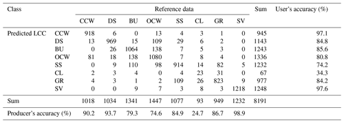
CCW: closed-canopy woodland. DS: dense scrubland. BU: bushland. OCW: open-canopy woodland. SS: sparse scrubland. CL: cultivated land. GR: grassland. SV: sparsely vegetated land.

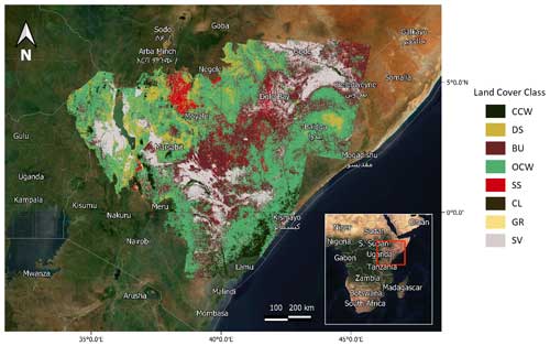
Figure 8 The 30 m resolution predicted land cover classification for 2015. Class codes and descriptions are presented in Table 1. Basemap: © MapTiler, https://www.maptiler.com/copyright/ (last access: 10 November 2023). Class codes correspond to the following: CCW – closed-canopy woodland, DS – dense scrubland, BU – bushland, OCW – open-canopy woodland, SS – sparse scrubland, CL – cultivated land, GR – grassland, SV – sparsely vegetated land.

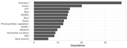
Figure 9 Variable importance derived from the best random forest classifier (see description of variables in Sect. 2.4.2).

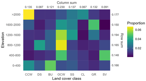
Figure 10 Proportion of reference data (81 419 total pixels) for each land cover class and 400 m elevation interval in our study area. Class codes correspond to the following: CCW – closed-canopy woodland, DS – dense scrubland, BU – bushland, OCW – open-canopy woodland, SS – sparse scrubland, CL – cultivated land, GR – grassland, SV – sparsely vegetated land.

After a sample of 108 locations for bare ground, 900 locations for NPV, and 900 locations for PV were established, the spectral information of the temporally closest Landsat image was extracted for its use in the endmember estimation. We estimated the endmembers from the spectral signatures of the sampled pure points using an R-based function for modeling of endmember compositions based on bilinear unmixing (Seidel and Hlawitschka, 2015; Weltje, 1997). We used blue, green, red, NIR, SWIR1, and SWIR2 bands as input spectral data for each point and established a convexity threshold of −6 and 10 000 iterations with a standard weighting exponent of 1, as suggested by Weltje (1997).

We used a pseudo-inverse unmixing algorithm on GEE with two constraints to calculate fractional covers. The first constraint forces the fractions to sum to 1; therefore each fraction represents an actual percentage of each class. The second constraint forces all fractional values to be non-negative. The resulting maps include three bands corresponding to each of the three calculated fractions.

2.5.1 Accuracy assessment of fractional cover

We used RCC classifications to assess the performance of our fractional cover estimations, as the RCC classifications provide very accurate measures of class fractions at the Landsat pixel scale. Using the results from the classifications performed over HR imagery, we aggregated the classified classes into vegetation, BG, and other (including impervious surfaces, water, and cloud classes). Since NPV is difficult to detect with available HR datasets, this aggregation permits a separation between vegetation classes (which logically include PV and NPV) and BG, since BG is the complementary proportion of vegetation when just the two classes occur (i.e., where there is no cloud obstruction, water or impervious surfaces, or: 1 − BG = PV + NPV). Second, we selected the temporally closest Landsat-based fractional cover layer to a subset of 10 RCC classifications. Third, we generated a layer of the centroids of pixels for these fractional cover estimates and randomly selected 5000 centroids. Fourth, we generated circles of 15 m radius (approximate size of Landsat pixels) at the locations of the sampled centroids and clipped the aggregated classification. From this sample, we only selected the circles fully overlapping vegetation and BG pixels. Fifth, we calculated the proportion of pixels of vegetation and BG within each circle. Finally, after completion of this process, we compared the values of these proportions to the Landsat-derived fractional cover using regression statistics: R², normalized root mean squared error (nRMSE) in units of percent cover, and p values.

3 Analysis

3.1 Land cover classification

Overall, the LCC procedure resulted in an overall accuracy of 85.57 %, with a kappa of 0.832, which is above the recommended threshold of 85 % for LCC predictions and remarkable for such a large area as our study area (Foody, 2002; see Fig. 8). The resulting confusion matrix from the accuracy testing partition of the 8191 randomly selected points is presented in Table 2. The random forest model using all bands was more accurate than that using subsets of input bands. In decreasing order, variable importance derived from the random forest classifier for every band was elevation, green, EVI, red, SWIR2, blue, slope, photosynthetic vegetation, SWIR1, MSAVI2, horizontal curvature, NIR, and bare ground (Fig. 9). The proportion of importance on the elevation covariate is almost double the next most important variable, the green band. Figure 10 shows the proportion of reference data, including training and validation sets, showing the apparent elevation segregation of the samples.

The annual time series of the total proportion of each land cover class in our study area shows variations in the proportion of SV, SS, and OCW classes around the same years within the studied time frame (Fig. 11). To understand the source of such variation, Fig. 12 presents the proportion of inter-annual transitions of each pixel from class to class for the study period. Potentially valid transitions are defined in our state-and-transition model, presented in Fig. 7. Using this model, we can use the potentially valid inter-annual transitions and compare them with all inter-annual transitions in each pair of subsequent years (only using unmasked pixels with class values in both years). Our expected, potentially valid, inter-annual state transitions between land cover classes (Fig. 7) were above 62.30 % in all yearly transitions (Fig. 12), with a mean of 75.20 % and a maximum of 83.20 %. The number of unmasked paired pixels as a proportion of the total Landsat-based pixels used for the calculation of land cover had a minimum of 86.60 %, with a mean of 95.30 %. Three drops in the number of valid transitions are visible in Fig. 12, which correspond to three drought events followed by rains and a greening effect on the landscape (Okal et al., 2020). This effect becomes evident while looking at the changing proportions of closed-canopy woodland (CCW) and sparse vegetation (SV) for 2005–2006, 2010–2011, and 2017–2019 in Fig. 11.

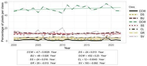
Figure 11 Annual time series of proportion of pixels of land cover classes for the entire study area (total 30 m pixel count = 858 780 117). Colored lines correspond to linear trends for each class over the study period.

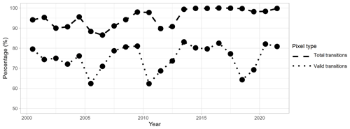
Figure 12 Proportion of pixels with potentially valid yearly transitions. Dashed and dotted lines show the total number of paired unmasked land cover classes and the total number of potentially valid transitions as per our state-and-transition model presented in Fig. 7.

Filtering out pixels with unlikely transitions as defined in our state-and-transition model allows us to reconstruct the history of individual pixels and help understand their change through time. The alluvial chart is a useful visualization to track such transitions through time by presenting the frequency distributions of classes in different time periods, aggregating the change of pixels with the same transitions between classes into individual ribbons. Figure 13 shows the decadal change of 48 280 randomly selected pixels with potential valid transitions and no missing data in our study area from 2000–2020. By assigning colors to the last year in the sequence, it is possible to visually track changes, evidenced by the width of the lines moving from one class to another between periods. The largest change of classes in this sample corresponds to 1.75 % of pixels (n = 845) staying as OCW in 2000 and 2010 but changing to CCW by the year 2020 (see dark ribbon going from OCW to CCW between 2010 and 2020). This is followed by 1.37 % of BU pixels (n = 661) turning into SV by the year 2010 and staying in that class until 2020 (see dark ribbon going from BU to SV between 2000 and 2010). Other classes present changes less than 1 %.

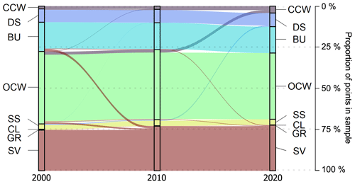
Figure 13 Decadal vegetation transition between 2000–2020 of 48 280 random pixels with potentially valid land cover transitions, as defined in our state-and-transition model for the 3 selected years. Land cover classes are presented in Table 1. Color codes were assigned to land cover classes present in the locations in year 2020 in order to track changes between decades.

3.2 Vegetation fractional cover estimation

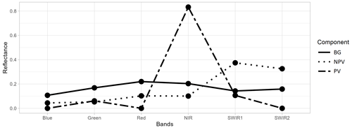
Endmember estimation reached the threshold convexity error of −6 after 3265 iterations, with total negative values representing just 0.026 % of the sample, reflecting excellent model fit and a very small proportion of sample points falling off the multidimensional space between endmembers (Weltje, 1997). Figure 14 shows the estimated spectral signatures of endmembers, where a large spike in NIR is visible for PV and high values of reflectance at the SWIR bands are also discernible for BG. Regression results from the comparison between bare-ground estimations from HR imagery and Landsat-based predictions yielded R²=0.795, p < $\mathrm{2.2}\times {\mathrm{10}}^{-\mathrm{16}}$, normalized root mean squared error (nRMSE) = 0.123, with equation y= 0.959 (SE = 0.010) x+5.768 (SE = 0.843), F = 9201.1 on 1, and 2152 DOF, with a p value of < $\mathrm{2.2}\times {\mathrm{10}}^{-\mathrm{16}}$ (Fig. 15).

Figure 14 Estimated spectral endmembers for fractional cover estimation.

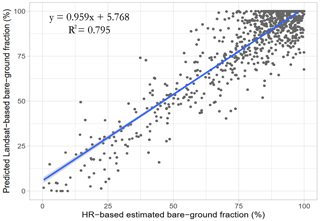
Figure 15 Spatial–temporal correlation between HR imagery and Landsat-based predictions of bare-ground fractional cover (n = 2190) at Landsat scale of 30 m from 2016 to 2020. F = 9201.1 on 1 and 2152 DOF, with a p value of < $\mathrm{2.2}\times {\mathrm{10}}^{-\mathrm{16}}$.

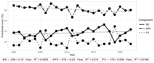
Final products consisted of yearly short, dry-season estimations of fractional cover for our entire AOI with a total of 858 780 117 pixels (Fig. 16). Further qualitative assessment of fractional cover predictions against natural-color Landsat images and compositions confirmed accurate representations of the ground conditions. The most readily identifiable components BG and PV show regional accordance with very dry and forested areas, respectively, within our AOI (Fig. 16). Similar to the LCC time series, fractional cover showed distinct variations in three different periods (Fig. 17).

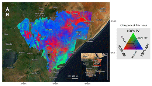
Figure 16 Landsat-derived 30 m resolution fractional cover estimations for the short, dry season of 2020, with mixtures of PV (photosynthetic vegetation), NPV (non-photosynthetic vegetation), and BG (bare ground) for our entire AOI (see legend on figure). Basemap: © MapTiler, https://www.maptiler.com/copyright/ (last access: 10 November 2023).

Figure 17 Annual time series of average fractional cover values for BG, NPV, and PV for the entire study area (pixel count = 858 780 117). Straight lines correspond to linear trends for each component over the study period.

4 Data availability

Our 30 m resolution annual land cover classification and fractional cover data are publicly available at https://doi.org/10.5281/zenodo.7106166 (Soto et al., 2023) and Google Earth Engine (see Appendix A).

5 Discussion

The dataset generated in this study represents a substantial improvement over previously available data to assess rangeland health in the region, such as plain NDVI from Landsat and MODIS products. These improvements are the result of a high spatial resolution, a long temporal extent, and use of land and fractional cover metrics expressly designed to inform monitoring and assessment of eastern African rangeland systems (e.g., Hill and Guerschman, 2022; Sexton et al., 2013; Buchhorn et al., 2020).

Our land cover classification scheme allowed us to reach acceptable per-class accuracy levels, using 85 % as a reference value for most of our land cover classes (Mundia and Aniya, 2005; Rogan et al., 2003; Treitz and Rogan, 2004; Weng, 2002; Yang and Lo, 2002), considering the limitations of both the availability of ground reference data and Landsat imagery. Our proposed method that used HR imagery to generate training and validation data for the Landsat-based classification has proven to be key to reaching these accuracy levels, enabling us to increase the amplitude of spectral information of the different features found across such a large and heterogeneous area. HR imagery also allowed us to have homogeneous spatial representation in ground-reference data as shown in Fig. 2, thus reducing biases from imbalanced sampling (Carlotto, 2009; Elmes et al., 2020). We also included a minimum threshold value for HR classifications and applied a ruled-based algorithm to generate training data, therefore helping to reduce and control our training data error (Elmes et al., 2020; Padial-Iglesias et al., 2021). Homogenization of the VPI process also helped standardize training data generation, accounting for the arising inconsistencies that might impact the Landsat LCC estimations (Elmes et al., 2020; Foody, 2009).

One limitation of our product is its comparatively lower classification accuracy for cultivated land areas. The close spectral correspondence between the dominant cultivated grain crops in the region (e.g., teff, maize and sorghum in Ethiopia) and wild grasses makes separation of the two challenging. In addition, other land classes such as sparse shrub could also be difficult to separate from cultivated land (Hansen et al., 2005; Sexton et al., 2013), because they are dominated by either PV or NPV during the short, dry season where our Landsat compositions were compiled. These two factors limit the applicability of the proposed approach to extensive rangeland areas. We encourage users of this dataset to explore the behavior of the CL class within their study areas before carrying out further analyses. In addition, cloud cover in this region implies that other tools such as dynamic time warping (Müller, 2007) might not improve land cover estimations, as this technique requires the extraction of temporal features from time series that are not possible to generate using Landsat imagery in our defined temporal extent. As with virtually all visible-light satellite-based remote sensing, cloud cover limits our analysis, reducing both the amount of per-pixel available imagery and also the proportion of pixels with available data over our study area. Other factors such as precipitation resulted in a > 30 % drop in accuracy due to increases in annual accumulated precipitation, as found in our preliminary classifications.

In addition to class-specific issues, the multi-year classification scheme used here has limitations and possible effects on the classification results on years without reference data, which can include misrepresentation of the real patterns. This study does not explore this effect due to the lack of in situ reference data for the total length of the studied period. However, other studies in similar ecosystems where reference data are available can help improve the products presented here or to find the possible biases they might have. Current research on the use of transfer learning, with the use of pre-trained models and fine-tuning with limited data, provides very good opportunities for further improvement of remote sensing products and possible bias exploration (e.g., Li et al., 2023; Račič et al., 2024; Weikmann et al., 2021).

As shown in Fig. 13, this dataset can not only provide descriptions of all the land cover pixel transitions of a given study area but also has the potential value of providing a foundation for assessments of long-term change trajectories that likely will extend beyond the time scope of the current study. Ecological studies on ecosystem and community dynamics require long-term ecological datasets (Ellis et al., 2006; Magurran et al., 2010; Ott et al., 2019). Further use of these products should demonstrate their usefulness as monitoring, prioritization, and inventory tools for planning and decision-making (Allred et al., 2022). Land cover mapping will enable the isolation of signals from rangelands and incorporate heterogeneity into management frameworks, providing foundations for assessments of long-term change trajectories that likely will extend beyond the time scope of the current study in this specific geographical region (Fuhlendorf et al., 2012).

Vegetation fractional cover estimates showed high accuracy. This accuracy is likely aided by the availability of HR imagery (Brandt et al., 2020) used for generation of ground reference data for training and validation. Even under our limitations on ground reference data, bare ground, a key indicator of rangeland health conditions for monitoring and management (Pellant et al., 2020; Rigge et al., 2019, 2020), was accurately identified over a relatively large area of more than 4.6×10⁶ ha. Figure 17 shows the potential value of this dataset by presenting a summarization of the annual trend of all three fractional components, which can be reconstructed from different spatiotemporal aggregations, down to the pixel level. Such trajectories will likely help understand the contributing factors for observed and unobserved patterns in the past two decades (Rigge et al., 2021). While further exploration of the spatial and temporal distribution of these trends is needed, this overall assessment might reflect a slow degradation of rangeland condition as bare-ground fraction gradually increases (Fig. 17).

Here, we used intensive algorithms on HR satellite imagery to allow training and assessment of the performance of our proposed methods, as little ground reference information exists in this vast and remote region. This approach helps to maintain enough detail on the land cover classes and allowed the creation of a relevant VFC estimation. Our maps could help generate new threads of rangeland maps for eastern Africa, especially to improve community development, ecological conservation, and humanitarian programming. As the lack of ground reference data has been a bottleneck to empirical rangelands research in this part of the world, our HR-based estimations can help develop and improve assessments of rangeland health trajectories. The increasing availability of remote sensing imagery and the application and development of new machine learning algorithms will certainly help develop better management tools. Relatively recent collections such as Sentinel-2 and its harmonization with Landsat imagery (Claverie et al., 2018) will need to be tested for their advantages and disadvantages for their use in long-term time series in this geographic area.

The framework proposed here of harnessing HR images to generate training labels in a semi-automatic procedure, including manual VPI and RCC to automatically create reference data based on class proportions, will become highly relevant considering recent technological advancements. Modern tools such as large language models (LLMs) and foundation models carry a huge promise to improve generalizability of this approach and classification accuracies in complex landscapes. With the future use of these new tools and fine-tuning, we expect our models specifically trained in our study domain to be generalizable to other dryland/rangeland regions in the whole of sub-Saharan Africa or other continents (e.g., Australia, parts of central Asia), where ecosystems, land cover compositions, herding intensities, and other similar features exist.

Overall, this dataset will be useful to monitor the impacts of different rangeland management practices or test the impact of development programs. The open access to sophisticated cloud computing platforms, such as GEE (Gorelick et al., 2017), will contribute to practical use and further assessment of this dataset. To accomplish this, have made these two products available in GEE (see “Data availability”).

Appendix A: Description of access to Google Earth Engine (GEE) data

Land cover classification data can be accessed using GEE's asset IDs with the following structure: projects/ee-gerardosoto/assets/lcClass< YEAR>. For example, for the year 2000, use “projects/ee-gerardosoto/assets/lcClass2000”.

Alternatively, use the GEE link as follows: https://code.earthengine.google.com/?asset=_projects/ee-gerardosoto/assets/lcClass2000 (last access: 10 November 2023).

Vegetation fractional cover data can be accessed using GEE's asset IDs with the following structure: projects/ee-gerardosoto/assets/fracCov< YEAR> _int16. For example, for the year 2000, use “projects/ee-gerardosoto/assets/fracCov2000_int16”.

Alternatively, use the GEE link as follows: https://code.earthengine.google.com/?asset=projects/ee-gerardosoto/assets/fracCov2000_int16 (last access: 10 November 2023).

Appendix B: Reference flash card sets

The following pages include the flash cards used to reference land cover types and canopy cover.

Figure B1 Flash card for land cover type “closed-canopy woodland”.

Figure B2 Flash card for land cover type “dense scrubland”.

Figure B3 Flash card for land cover type “bushland”.

Figure B4 Flash card for land cover type “open-canopy woodland”.

Figure B5 Flash card for land cover type “sparse scrubland”.

Figure B6 Flash card for land cover type “cultivated land”, maize crop.

Figure B7 Flash card for land cover type “cultivated land”, cropped versus fallow.

Figure B8 Flash card for land cover type “cultivated land”, teff crop.

Figure B9 Flash card for land cover type “grassland”.

Figure B10 Flash card for land cover type “sparsely vegetated land”.

Figure B11 Flash card for canopy cover level “2 m diameter in a 30 by 30 m plot”.

Figure B12 Flash card for canopy cover level “4 m diameter in a 30 by 30 m plot”.

Figure B13 Flash card for canopy cover level “8 m diameter in a 30 by 30 m plot”.

Figure B14 Flash card for canopy cover level “2 m diameter in a 10 by 10 m plot”.

Figure B15 Flash card for canopy cover level “4 m diameter in a 10 by 10 m plot”.

Figure B16 Flash card for canopy cover level “8 m diameter in a 10 by 10 m plot”.