A spectral–structural characterization of European temperate, hemiboreal, and boreal forests

Radiative transfer models of vegetation play a crucial role in the development of remote sensing methods by providing a theoretical framework to explain how electromagnetic radiation interacts with vegetation in different spectral regions. A limiting factor in model development has been the lack of sufficiently detailed ground reference data on both the structural and spectral characteristics of forests needed for testing and validating the models. In this data description paper, we present a dataset on the structural and spectral properties of 58 stands in temperate, hemiboreal, and boreal European forests. It is specifically designed for the development and validation of radiative transfer models for forests but can also be utilized in other remote sensing studies. It comprises detailed data on forest structure based on forest inventory measurements, terrestrial and airborne laser scanning, and digital hemispherical photography. Furthermore, the data include spectral properties of the same forests at multiple scales: reflectance spectra of tree leaves and needles (based on laboratory measurements), the forest floor (based on in situ measurements), and entire stands (based on airborne measurements), as well as transmittance spectra of tree leaves and needles and entire tree canopies (based on laboratory and in situ measurements, respectively). We anticipate that these data will have wide use in testing and validating radiative transfer models for forests and in the development of remote sensing methods for vegetation. The data can be accessed at Hovi et al. (2024a, https://doi.org/10.23729/9a8d90cd-73e2-438d-9230-94e10e61adc9) (for laboratory and field data) and Hovi et al. (2024b, https://doi.org/10.23729/c6da63dd-f527-4ec9-8401-57c14f77d19f) (for airborne data).

1 Introduction

Remote sensing of vegetation, and of forests in particular, has experienced significant growth in recent years (e.g., Fassnacht et al., 2024) due to advancements in sensor technology, data processing and interpretation techniques, and new satellite missions (such as PRISMA, EnMAP, CHIME, and SBG). At a global level, remote sensing can provide information about pressing global issues such as the connections between climate change and vegetation dynamics (e.g., Piao et al., 2020) and support for biodiversity conservation (e.g., Pettorelli et al., 2016). Furthermore, at finer spatial scales, optical remote sensing allows detailed and accurate monitoring of, for example, vegetation productivity, diversity, and health (e.g., Kooistra et al., 2024; Hernández-Clemente et al., 2019).

Radiative transfer (RT) models of vegetation play a crucial role in the development of remote sensing methods by providing a theoretical framework to explain how electromagnetic radiation interacts with vegetation in different spectral regions (Ross, 1981; Myneni and Ross, 1991). Based on mathematical formulations, these models allow us to understand and quantify the complex interactions between radiation and canopy components, such as leaves and stems, and the underlying soil (Liang, 2004). By modeling the radiative transfer processes, it is possible to explain the spectral signatures observed by remote sensing instruments under different environmental and illumination conditions or to support future sensor design and planning of data collection strategies (e.g., Vicent et al., 2015).

RT models and other physically based canopy reflectance and transmittance models have been developed for over 3 decades. For forests, these models (e.g., Gastellu-Etchegorry et al., 1996; North, 1996; Kuusk and Nilson, 2000; Leblanc and Chen, 2000) are often more complicated and require a larger number of input variables than models for other vegetation ecosystems (e.g., Jacquemoud et al., 2009; Verhoef, 1984) due to the complex tree canopy architecture and subsequent multiple interactions of photons both within and between canopy elements and between the forest floor and the canopy (e.g., Stenberg et al., 2008). Even though there are modeling approaches that require a smaller number of input variables for forests (Stenberg et al., 2016), a limiting factor in model development has been the lack of extensive or sufficiently detailed ground reference data on both the structural and spectral characteristics of forests needed for testing and validating the models. This lack of data affects both model developers and larger scientific frameworks, such as the RAdiation transfer Model Intercomparison (RAMI) initiative (Gobron et al., 2023). While structural data on forests (e.g., tree height, crown length, number of trees per ground area, canopy cover, leaf area index) are commonly available from sources such as forest inventory databases, spectral data on forest components (e.g., leaf or forest floor reflectance and/or transmittance spectra) are less frequently accessible. In addition, some structural properties (e.g., clumping index) that are relevant for RT models are also not commonly available but can be derived from detailed structural measurements.

To date, major efforts in collecting ground reference data that can be used in radiative transfer models for forests have focused on the North American continent. For instance, projects like the National Ecological Observatory Network (NEON) (NEON, 2024) and the Boreal Ecosystem-Atmosphere Study (BOREAS) (Sellers et al., 1997) offer input data for developing RT modeling for forests. While these initiatives have primarily aimed to understand ecosystem dynamics, their datasets also include key variables needed for RT models. For testing and validating forest RT models in European forests, there is only a small number of datasets that include the necessary structural and spectral information across various scales (e.g., Kuusk et al., 2009; Widlowski et al., 2015; Schneider et al., 2017; Liu et al., 2023). Furthermore, these datasets are limited in size, containing information on only a few forest stands. Even though various solutions have been suggested to overcome the lack of input data for RT models by using data from multiple sources (e.g., Malenovský et al., 2019), the lack of missing primary data persists. In addition to having to collect the data from multiple sources representing different time periods or geographical locations, these datasets are often not openly available according to FAIR (Findable, Accessible, Interoperable, Reusable) data principles (Wilkinson et al., 2016).

In this data description paper, we present a unique, open dataset on the structural and spectral properties of 58 stands in temperate, hemiboreal, and boreal European forests collected during a project funded by the European Research Council. The dataset is specifically designed for the development and validation of radiative transfer models for forests but can also be utilized in other remote sensing studies. It comprises detailed information on forest structure based on forest inventory measurements, terrestrial and airborne laser scanning, and digital hemispherical photography. Furthermore, the dataset includes spectral properties of the forests at multiple scales: reflectance spectra of tree leaves and needles (based on laboratory measurements), the forest floor (based on in situ measurements), and entire stands (based on airborne measurements), as well as transmittance spectra of tree leaves and needles and entire tree canopies (based on laboratory and in situ measurements, respectively). For distributing the data, we selected open, widely available formats. The dataset follows the FAIR principles.

2 Data collection

2.1 Study sites

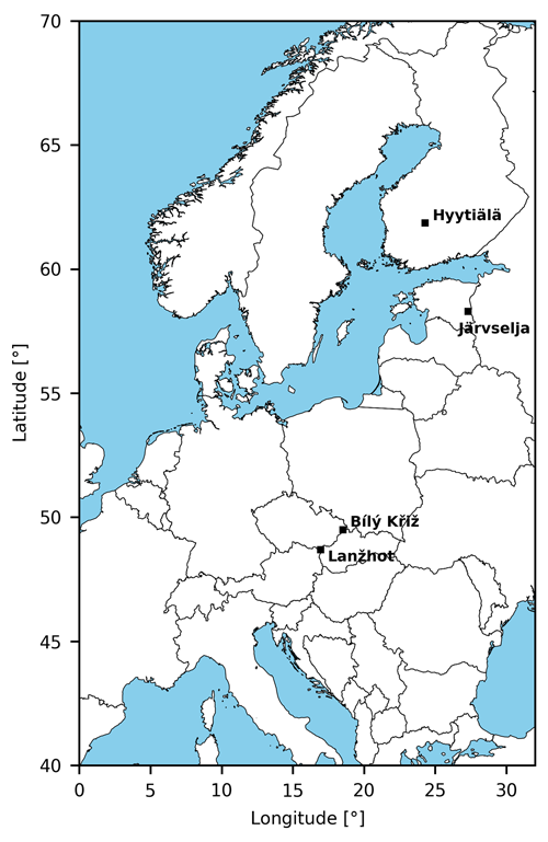
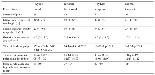
We collected data from 58 forest stands representing different forest structures and species compositions in temperate, hemiboreal, and boreal forests of Europe during the summers of 2019–2021 (Table 1, Fig. 1). The sites in Finland and the Czech Republic (Hyytiälä, Lanžhot, Bílý Kříž) are part of the Integrated Carbon Observation System (ICOS), which means that time series of meteorological and other ecosystem data are also openly available. The site in Estonia (Järvselja) also has a tower system for measuring variables related to atmosphere–biosphere interactions, and the data are available, on request, from the tower manager. We have summarized information on the study sites in Table 1, and we provide a short verbal description of them in the following text.

Figure 1 A map showing the locations of the study sites.

Our boreal study site, Hyytiälä, was located in Finland (61°51^′ N, 24°18^′ E) and is a moderately flat (130–200 m a.s.l.) area dominated by coniferous tree species. The forest floor is dominated by dwarf shrubs, graminoids, mosses, or lichens. Bare soil is rarely visible. Field measurements in Hyytiälä were conducted during 2019 and 2021.

Our hemiboreal site, Järvselja, was located in Estonia (58°17^′ N, 27°19^′ E) and is a flat (30–45 m a.s.l.) area with mixed broadleaved and coniferous forests. The forest floor is dominated by shrubs, dwarf shrubs, graminoids, and mosses. Bare soil is rarely visible. Field measurements in Järvselja were conducted during 2020.

Our temperate study sites, Lanžhot and Bílý Kříž, were located in the Czech Republic. Lanžhot (48°41^′ N, 16°57^′ E) is a temperate broadleaf-dominated floodplain forest area (ca. 150 m a.s.l.). The forest floor is sparsely covered by graminoids and shrubs, and decomposed plant materials (or bare soil) is commonly visible due to a high game density. Bílý Kříž (49°30^′ N, 18°32^′ E), on the other hand, is a temperate coniferous mountain forest area (700–950 m a.s.l.) where the forest floor is dominated by dwarf shrubs, graminoids, and mosses. Field measurements in the Czech sites were conducted during 2019.

Table 1 Summary of the study plots and measurement campaigns.

2.2 Overview of measurement campaigns

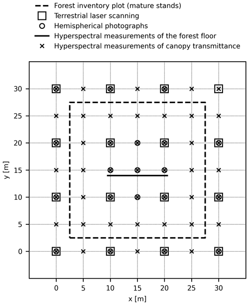
We established 28 plots in Hyytiälä, 13 in Järvselja, 10 in Lanžhot, and 7 in Bílý Kříž (Fig. 2). Each plot was located within a homogeneous forest stand with a minimum distance of 30 m from the plot center to the stand border, to ensure that uncertainties in geolocation would not impact the interpretation of commonly used medium-spatial-resolution optical satellite data. The same sampling and measurement protocols were applied in collecting field data in all study sites. Photographs from the measurement campaigns are available in Appendix A (Fig. A1) and in the published datasets. Note that we apply the reflectance terminology outlined by Schaepman-Strub et al. (2006) for the field and laboratory spectral measurements described in this paper.

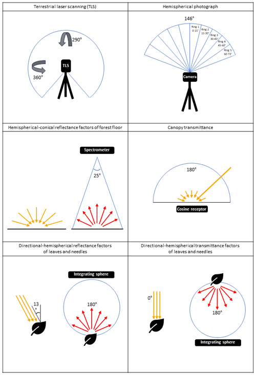
In all plots, we carried out forest inventory (Sect. 2.3.1) and terrestrial laser scanning (Sect. 2.3.2), took hemispherical photographs of the tree canopy (Sect. 2.3.3), and conducted spectral measurements and estimation of the vegetation fractional cover of the forest floor layer (Sect. 2.3.4). In addition, we measured the spectral transmittance of tree canopies in a subset of plots (Sect. 2.3.5) and measured the reflectance and transmittance spectra of the foliage of dominant tree species in all study sites (Sect. 2.3.6). The illumination and view geometries of the sensors during the field measurements are provided in Appendix A (Fig. A2). An airborne measurement campaign was conducted at all study sites to obtain contemporaneous hyperspectral (Sect. 2.4.1) and laser scanning data (Sect. 2.4.2). The same aircraft and instrumentation were used for the acquisition of airborne data in all measurement campaigns. The datasets are provided by Hovi et al. (2024a) and Hovi et al. (2024b).

Figure 2 A diagram showing the sampling design for field measurements described in Sect. 2.3.

2.3 Field datasets

2.3.1 Forest inventory

We conducted forest inventory measurements to obtain detailed information on the tree species and stand structure and took photographs of each plot at six fixed locations to provide an overview of the forests for data users. The fixed locations were all four corners of the plot and in the center of the plot (in two different directions). The forest inventory was carried out with distinct protocols for mature stands (D>10 cm) and young stands (D<10 cm), categorized based on the average diameter at 1.3 m height (D) for trees. For simplicity, we refer to stands with D>10 cm as mature stands and those with D<10 cm as young stands.

In mature stands (number of plots, n=44), a tree-wise inventory was performed within a rectangular area measuring 25 m × 25 m (Fig. 2). The diameter at 1.3 m height was measured using a caliper, and the tree species were identified for every tree exceeding a predetermined diameter threshold. The thresholds were determined in relation to the average tree height in the plot (h) and were as follows: 8 cm if h>16 m, 5 cm if 10 m $\le h\le \mathrm{16}$ m, and 2.5 cm if h<10 m. Tree height was measured with a Vertex ultrasonic hypsometer for two trees (median trees of thickest 10 % of trees) in each plot. These plots had 16 terrestrial laser scanning (TLS) points (see Sect. 2.3.2).

In young stands (n=6), 16 circular sub-plots were measured, arranged in a 4×4 grid with a 10 m distance between grid points (see TLS grid in Fig. 2). The area of each sub-plot was 25 m² (i.e., having a radius of 2.82 m). Within each sub-plot, the number of trees per species and the diameter and height of the median tree per species were measured. These plots had one terrestrial laser scanning (TLS) point (see Sect. 2.3.2).

An exception to the forest inventory protocol was made only in Hyytiälä for the plots (n=8) measured in 2021, where relascope sampling was used to determine whether a tree belonged to the plot or not. The diameter at 1.3 m height was measured for all sampled trees, and tree height was measured for the median tree per species. These plots had one terrestrial laser scanning (TLS) point (see Sect. 2.3.2).

Descriptive forest characteristics were derived from the forest inventory data for each study plot. These include number of stems per hectare, basal area, tree species proportions, and tree dimensions (i.e., stem diameter and tree height). A more accurate description of the calculation of these variables is provided in the README file of the data. In forest inventory measurements, typical uncertainties (standard deviation) for diameter at breast height and tree height are 0.3 cm and 0.5 m, respectively (Luoma et al., 2017).

2.3.2 Terrestrial laser scanning (TLS)

We collected TLS data that can be used to characterize the 3D geometry of the forest canopies in all plots, comprising a total of ∼2800 individual trees. The Leica P40 ScanStation, utilized in our study, operates at a wavelength of 1550 nm. It has a 6 mm beam diameter at the source and a 0.23 mrad beam divergence. The scan resolution equaled the beam divergence (i.e., 0.23 mrad or around 0.013°). The only exceptions to this were the measurements (1) in Hyytiälä in 2021 (n=8) and (2) in young stands in Järvselja (n=4), where the scan resolution was 0.31 mrad (0.018°). These exceptions are clearly labeled in the dataset.

There were two alternative sampling strategies for collecting TLS data. The choice of sampling approach was based on stand density at a height of 1–2 m above ground to avoid occlusion of co-registration targets and time constraints. In 44 plots, TLS scans were conducted at 16 grid points (Fig. 2), corresponding to the mature forest category described in Sect. 2.3.1. In 14 plots, TLS scans were conducted only at a single location (at the center of the plot, Fig. 2).

Scans were exclusively carried out under calm wind conditions (under 4 m s⁻¹ in 16-scan plots, under 8 m s⁻¹ in single-scan plots) and in dry weather. The scanning heights ranged from 1.4 to 1.8 m above the ground. In plots that had 16 scan positions, co-registration of scans was done using 25 polystyrene sphere targets, mounted on 1.5 m tall sticks placed within the plot area (Fig. 2). The co-registration errors were below 1 cm. All processing was done with the Leica Cyclone software.

The point clouds are intended for spatial modeling of canopy structure based on ray tracing rather than morphological modeling. Therefore, no filtering was applied at any stage of the data processing to preserve information. The TLS data in plots with 16 scans are available as full-resolution data, with each individual scan's point cloud stored separately, along with the transformation parameters of the co-registration. For viewing purposes, we merged and downsampled the point clouds to an average point spacing of 2 cm in Leica Cyclone and cropped the plot to an area of approximately 35 m × 35 m for the plots that had 16 grid (scanning) points. For the single-scan plots, the downsampled point cloud includes all data. The downsampled and merged point clouds are provided in the LAS format.

2.3.3 Hemispherical photographs

We also obtained a characterization of the tree canopies with hemispherical photography. Hemispherical photographs were taken in each plot under diffuse illumination and windless or calm wind conditions with a Nikon D5000 digital camera equipped with a geometrically calibrated lens (Sigma EX 4.5 mm f/2.8 DC HSM). The photographs were captured at 21 locations in each plot (Fig. 2) with the camera lens looking directly upwards. The camera was positioned at a height of 1.5 m when the mean tree height in a stand was over 10 m and at a height of 1.0 m in other forests.

The photographs were recorded in the best-quality 8-bit JPEG format. We manually adjusted the exposure time based on the illumination conditions and also took photographs with exposure times one stop higher and lower than the original, thus doubling and halving the exposure time. In the processing of the photographs, we selected the one where the pixel values in the blue band of the JPEG images filled the 8-bit dynamic range well without saturating the histogram, but the other photographs are also included in the dataset.

These hemispherical photographs served as the basis for estimating effective plant area index (PAI_eff) and canopy gap fractions at different viewing angles. Initially, the JPEG photographs were binarized according to Nobis and Hunziker (2005). Next, effective PAI was calculated based on gap fractions determined for five concentric rings, each with median zenith angles of 10.7, 23.7, 38.1, 52.8, and 66.6°. This method closely followed the one presented in the manual of the LAI-2200 Plant Canopy Analyzer (LI-COR, 2012), with minor variations in the zenith angles (as listed above). The systematic uncertainties in the gap fractions estimated from hemispherical photographs are less than 0.02. This estimate is based on a comparison to the spectral canopy transmittance measured at 450 nm (Sect. 2.3.5).

2.3.4 Hyperspectral measurements and other characteristics of the forest floor

We measured the spectral properties of the forest floor and estimated the fractional cover of different components forming the forest floor in all plots. The composition of the forest floor ranged from nearly bare soil or litter to dense green vascular or moss vegetation.

Hemispherical–conical reflectance factors (HCRFs) of the forest floor (ranging from 350 to 2500 nm) were measured in a central location in each plot using an Analytical Spectral Devices (ASD) FieldSpec4 spectrometer (serial no. 18456) with a 25° field of view. The initial spectral resolution ranged from 3 nm (for wavelengths ≤1000 nm) to 10 nm (for wavelengths >1000 nm); the sampling interval was 1.4 and 1.1 nm for visible and near-infrared (VNIR) and shortwave infrared (SWIR), respectively; and the instrument interpolated and outputted the data at 1 nm intervals. Please note that the same details on spectral resolution also apply to the data measured by the spectrometers described later in Sect. 2.3.5 and 2.3.6. Measurements were consistently conducted under diffuse illumination conditions so that the influence of unstable illumination conditions on the forest floor (i.e., sun flecks, shadows) could be avoided and so that the data collected at different latitudes and times of the day would be comparable. Preparations for the measurements included a warm-up period for the spectrometer lasting at least 30 min.

In each plot, we established a 11 m long east–west-oriented transect and made a total of 15 measurements at intervals of approximately 80 cm (Fig. 2). Measurements were recorded in the nadir direction from a height of approximately 1.3 m. For calibration, white reference measurements of a 25 cm × 25 cm Spectralon panel (with a nominal reflectance of 99 %) were conducted at both ends of the transect, as well as at every third measurement point along the transect. Dark current measurements were taken at both ends of the transect. The integration time, offset, and gain of the spectrometer were adjusted based on illumination conditions using automatic optimization.

Raw radiation signals (i.e., digital numbers, DNs) were processed into hemispherical–conical reflectance factors (HCRFs), and the 15 pointwise measurements were averaged to produce a single spectrum per forest plot. We calculated the HCRF for each measurement point by dividing the DN value of the forest floor by the DN value of the Spectralon panel and multiplied this ratio with the reflectance of the white reference panel. Dark current readings were subtracted from all DN values prior to the calculation. Because white reference readings were made at every third measurement point, we performed a linear interpolation (in time) of the white reference measurements to obtain a value for all measurement points. The preprocessed data are provided in the CSV format. We estimated that these measurements have an uncertainty of ∼10 % due to variations in illumination conditions.

Fractional cover was defined as the fraction of ground covered by living or dead plant material or lichens in 1 m² vegetation quadrats. Fractional cover was estimated for all plots from nadir-view RGB (red, green, blue) photographs (four per plot) taken by a Nikon D5000 camera at every fourth spectral measurement point (at a height of 1.5 m) along the transect where spectral measurements were made. A wooden frame of 1 m × 1 m was placed at these measurement points, and the entire frame (vegetation quadrat) was included in the photograph. After field work, the photographs were processed to obtain estimates of fractional cover. The frame in each photograph was superimposed with a 10×10 grid, where each grid cell represented 1 % of the total image area. The forest floor present in each grid cell was visually classified into one of the following classes: (1) vascular plants, (2) non-vascular plants (i.e., mosses), (3) lichen, (4) intact plant litter, or (5) decomposed plant litter. The criterion for selecting one of the classes was that it was the most abundant class in the grid cell. Finally, the fractional cover of each class in the photograph was determined by aggregating the grid-cell-specific results, and the average fractional cover of each forest floor class within a forest plot was determined by calculating the mean of the fractional cover values across the four photographs.

2.3.5 Hyperspectral measurements of canopy transmittance

We conducted measurements of the spectral transmittance of tree canopies (ranging from 350 to 2500 nm) in eight plots in Hyytiälä, six plots in Järvselja, four plots in Lanžhot, and four plots in Bílý Kříž. Spectral transmittance of a canopy was defined as the ratio of below-canopy spectral radiation flux to above-canopy spectral radiation flux.

For these measurements, we used two FieldSpec3 or FieldSpec4 spectrometers and two identical cosine receptors (diffuser type, model A124505) manufactured by ASD. In each forest plot, spectral transmittance was measured at 49 locations (Fig. 2). The ASD FieldSpec4 spectrometer (serial no. 18456) was consistently employed for measurements within the forest (i.e., below-canopy), whereas the ASD FieldSpec3 or FieldSpec4 (serial no. 18641 or 16089) served as a reference spectrometer (i.e., above-canopy). For the above-canopy measurements, a tripod was used to affix the cosine receptor which was measuring at 15 s intervals in an open area within the study site (within <2 km distance from the plots). Measurements were conducted only under cloud-free conditions, with solar elevation angles ranging from 30 to 45°.

Preparations for the measurements included a warm-up period for the spectrometers lasting at least 30 min, automatic optimization of the spectrometers' integration time and gain settings, and an intercalibration of the two spectrometers. The intercalibration took place at the beginning and end of each measurement period (max 3 h 20 min). This involved placing the cosine receptors next to each other in an open area and conducting 10 measurements, with each measurement comprising 30 averaged spectra from both spectrometers.

After the field campaign, the data were processed into canopy spectral transmittance (T) as

$$\begin{array}{}\text{(1)}& T={\displaystyle \frac{f_{\mathrm{bc}}{s}_{\mathrm{bc}}}{f_{\mathrm{ac}}{s}_{\mathrm{ac}}}}k,\end{array}$$

where s_bc and s_ac are raw signal (DN) values recorded below and above the canopy, respectively; k is the ratio of DNs measured by the two spectrometers under identical irradiance conditions (obtained from the intercalibration measurements); and f_bc and f_ac are correction factors that take into account possible changes in the integration time (at wavelengths up to 1000 nm) or the detector gain (at wavelengths above 1000 nm) due to re-optimization of either of the spectrometers during the measurement period. Re-optimization was needed if signal saturation occurred, for example, when measuring before noon as the solar irradiance increased towards noon. All quantities in the equation are wavelength- or detector-dependent. We estimated that these measurements have an uncertainty of ∼5 % due to variations in clear-sky illumination conditions.

2.3.6 Hyperspectral measurements of tree leaves and needles

We measured the directional–hemispherical reflectance factors (DHRFs) and directional–hemispherical transmittance factors (DHTFs) ranging from 350 to 2500 nm of leaves and needles for 15 dominant tree species within the study sites, adding up to a total of 1314 samples. The two coniferous tree species that we sampled were Norway spruce (Picea abies (L.) H. Karst.) and Scots pine (Pinus sylvestris L.). The 13 broadleaved tree species that we measured were common hazel (Corylus avellana L.), English oak (Quercus robur L.), European alder (Alnus glutinosa (L.) Gaertn.), European ash (Fraxinus excelsior L.), European aspen (Populus tremula L.), European hornbeam (Carpinus betulus L.), European Turkey oak (Quercus cerris L.), goat willow (Salix caprea L.), hedge maple (Acer campestre L.), little-leaf linden (Tilia cordata Mill.), silver birch (Betula pendula Roth), white poplar (Populus alba L.), and willows (Salix sp.). For simplicity, we will refer to leaves and needles collectively as foliage in the following text.

The foliage samples were measured in laboratory conditions using ASD RTS-3ZC integrating spheres which were equipped with a 10 W collimated halogen light source. The integrating sphere was coupled with an ASD spectrometer (FieldSpec3, serial no. 16089, or FieldSpec4, serial no. 18456 or 18641). Preparations for the measurements included a warm-up period for the spectrometer lasting at least 30 min.

In all study sites, visibly healthy foliage samples were obtained from both sun-exposed positions in the top of the canopy and shaded positions in the bottom of the canopy using professional tree climbers, towers, or long pruning shears. After cutting a branch from the tree, it was stored in a cool environment (with a maximum storage time of 12 h) and maintained with adequate watering, and foliage was removed from the branch immediately before the spectral measurements.

For coniferous trees, two age cohorts of needles were always sampled: current-year (c0) and 1-year-old (c1) needles. The position on a branch and the color of the needles and bark of the shoot, are macroscopic criteria that were used to recognize c0 shoots and needles. The c1 shoots were recognized by the presence of dead and partially shed bud scales at the base of the c0 shoot. In Hyytiälä, Järvselja, and Bílý Kříž, three trees representing each tree species were sampled, with three samples collected for each foliage class in each tree. This means that, for all tree species, we sampled sun-exposed c0 and shaded c0 foliage samples, and for conifers, we also sampled sun-exposed c1 and shaded c1 foliage classes. For less common broadleaved species in Järvselja (European ash, goat willow, little-leaf linden, common hazelnut, and unspecified willow), samples from one tree were obtained, and three sun-exposed c0 leaves were collected per tree species. In Lanžhot, one to four trees were selected for sampling. Each tree contributed one sample for every foliage class, including shaded c0 or sun-exposed c0.

For the duration of the spectral measurements of a sample in Hyytiälä, Järvselja, and Bílý Kříž, the sample (i.e., a leaf or a set of 7–10 needles) was fixed in a custom-made sample holder (see Fig. 1 in Hovi et al., 2020, for sample holder design) that was then fastened to the integrating sphere. Needles were arranged in the sample holder with a spacing of 0.5–1 times the width of a single needle (as recommended by Yáñez-Rausell et al., 2014), and leaves were placed so that major veins were not included in the measured spot. In Lanžhot, leaves of broadleaved species were not attached to sample holders.

We conducted measurements of DHRF and DHTF on both sides of the sample (corresponding to adaxial and abaxial in broadleaved species), along with white reference measurements for both DHRF and DHTF. A photon trap was used in the reflectance measurements to assess stray light. Our white reference was a Spectralon panel with 99 % nominal reflectance. The raw data were processed to derive leaf or needle DHRF and DHTF for all samples. For brevity, we denote DHRF with R and DHTF with T in the following equations:

$$\begin{array}{}\text{(2)}& {\displaystyle }R={\displaystyle \frac{s_R}{s_{\mathrm{ref},R}}}{\displaystyle \frac{\mathrm{1}}{\mathrm{1}-P_{\mathrm{gap},R}}}{R}_{\mathrm{ref}},\text{(3)}& {\displaystyle }T=\left({\displaystyle \frac{s_T}{s_{\mathrm{ref},T}}}-P_{\mathrm{gap},T}\right){\displaystyle \frac{\mathrm{1}}{\mathrm{1}-P_{\mathrm{gap},T}}}{R}_{\mathrm{ref}},\end{array}$$

where s_Rand s_T represent the raw signals (DN) obtained from the DHRF and DHTF measurements. Similarly, s_ref,R and s_ref,T denote the DNs from the white reference measurements for DHRF and DHTF, respectively. R_ref indicates the reflectance of the white reference panel, while P_gap,R and P_gap,T denote the gap fractions in the sample. Before R was computed, stray light was first subtracted from s_R and s_ref,R. DHRF includes specular reflection.

For broadleaved species, the gap fraction was assigned a value of 0 in the above calculations. Coniferous samples, on the other hand, included gaps between needles, and, thus, we determined the gap fractions using a digital film scanner (Epson Perfection V550, 800 dpi resolution). The detailed procedure for the determination of gap fraction was done according to Hovi et al. (2020). Finally, to address a slight inherent bias in DHTF measurements with the ASD RTS-3ZC integrating sphere (reported by Hovi et al., 2020) and to ensure that the sum of DHRF and DHTF did not exceed the one in the near-infrared (NIR) region, we implemented an empirical correction in which the DHTF spectra were multiplied with a correction factor of 0.945. Maximum uncertainty in the spectral measurements of foliage generally corresponds to the maxima of biological variation (Petibon et al., 2021). For coniferous (non-flat) needles, the errors are approximately 4 %–6 % in DHRF and 10 %–12 % in DHTF (Yáñez-Rausell et al., 2014).

For data users, we provide the spectra for all samples, as well as analysis-ready datasets. The analysis-ready datasets contain (i) the mean DHRF and DHTF spectra and their standard deviations for all tree species, canopy positions (top and bottom), needle age classes (c0, c1), and study sites and (ii) plot-specific mean DHRF and DHTF spectra which have been weighted based on tree species and needle age class proportions (i.e., computed from i).

2.4 Airborne datasets

2.4.1 Hyperspectral data

We arranged flight campaigns in mid-July 2019 in Hyytiälä and Järvselja and in early September 2019 in Lanžhot and Bílý Kříž (Table 1), representing green phenological conditions. Airborne hyperspectral measurements were collected across all study sites using the CASI-1500 and SASI-600 hyperspectral push-broom sensors from ITRES Ltd., Canada, mounted on a Cessna C208B aircraft which is part of the Flying Laboratory of Imaging Systems (FLIS) operated by the CzechGlobe Global Change Research Institute (Hanuš et al., 2023). The CASI-1500 covered visible (VIS) to NIR wavelengths (382 to 1052 nm), while the SASI-600 sampled NIR and shortwave-infrared (SWIR) wavelengths (958 to 2443 nm). Both sensors had a sampling interval and spectral resolution of 15 nm and underwent spectral and radiometric calibration prior to the flight campaigns in March 2019.

During the flight campaigns, the aircraft flew at an altitude of approximately 1 km above ground level. This yielded ground pixel sizes of 0.5 m (CASI) and 1.25 m (SASI). The CASI and SASI data were acquired in near-nadir observation geometry with a ±20° field of view. The flying azimuth direction closely matched the solar azimuth – the purpose of this was to reduce potential spectral differences within the same study site caused by reflectance anisotropy of forests in the solar principal plane. During acquisitions, the sun zenith angle ranged from 37 to 60°, and flight lines overlapped by 60 %–80 %.

The raw DN data from the hyperspectral sensors underwent initial radiometric correction with the RADCOR software (version 11) produced by ITRES Ltd. Subsequently, geo-orthorectification was performed using GEOCOR (version 5.6). The data were orthorectified to a surface model, which represents the top of the canopy in vegetated areas and the ground elevation elsewhere. Atmospheric correction was carried out with the ATCOR-4 software bundle (version 7.2.0 or 7.3.0), employing a database of atmospheric look-up tables generated with the MODTRAN5 radiative transfer code. In this correction, sensor measurements were adjusted for path and adjacency radiances. In-flight radiometric (vicarious) calibration was conducted for each site using a known bright reflectance target. Spectral bands highly affected by water vapor in the atmosphere (i.e., 895–1003, 1092–1168, 1302–1528, and 1737–2038 nm) were nonlinearly interpolated and depended on local atmospheric conditions. The parameters used in the atmospheric correction were retrieved directly from the airborne hyperspectral data. However, for the Hyytiälä site, the parameters were estimated from the on-site AERONET station (CIMEL sun photometer). No topographic correction was applied. The data produced through this processing chain are provided as at-surface (also called top-of-canopy) hemispherical–directional reflectance factors (HDRFs). We estimated that the uncertainty in the HDRF data (assessed as the deviation between the atmospherically corrected airborne data and the ground-measured spectra of reference targets) was less than 2 % in all wavelengths.

Finally, we inspected the CASI and SASI data manually to remove clouds or cloud shadows from areas corresponding to our study plots. During the flights, clouds were intermittently present over the Hyytiälä site and occasionally over the Bílý Kříž site. The Lanžhot and Järvselja flights, on the other hand, had cloudless conditions. Nearest-to-nadir cloud-free data from a 100 m × 100 m area around each plot were extracted and serve as an analysis-ready dataset. In addition, data from the entirety of the study sites are provided. These data cover approximately 4 km × 4 km areas in Hyytiälä and Järvselja, a 2 km × 3 km area in Lanžhot, and a 2 km × 2 km area in Bílý Kříž.

2.4.2 Laser scanning data (ALS)

Airborne laser scanning (ALS) data were collected simultaneously with the airborne hyperspectral data using a RIEGL LMS-Q780 laser scanner (RIEGL GmbH, Austria) mounted on the same Cessna aircraft. The laser scanner operated at a wavelength of 1064 nm and had a 0.25 mrad beam divergence and a maximum scan zenith angle of 30°. The pulse density at the study plots was 48, 32, 10, and 9 pulses m⁻² in Hyytiälä, Järvselja, Lanžhot, and Bílý Kříž, respectively. The differences between sites stem from different overlaps of flight lines. In Hyytiälä, the elevated pulse density was also partly due to repeated flight lines due to occasional cloud cover. The lowest absolute positional accuracy (RMS 27 cm) is associated with coordinates for off-nadir points acquired at the edges of the flight lines. The calculation of this accuracy is based on the performance of each component provided by the manufacturer and an acquisition height of 1030 m above ground. The raw waveform data were processed into point cloud format using RiPROCESS (version 1.8.4), RiANALYZE (version 6.2.2), RiWORLD (version 5.1.3), and GeoSysManager (version 2.0.8) software. We also computed raster digital elevation models with a pixel size of 1 m, by interpolating from the ground points classified with LAStools software. Similarly to the airborne hyperspectral data, analysis-ready data were extracted for a 100 m × 100 m area around each study plot, and the data are also provided for the entirety of the study sites as original point clouds and denoised data. Denoised data were processed to filter out points originating from the sky (due to, e.g., clouds) or false points under ground.

Table 2 Ancillary datasets relevant for RT modeling of forests available for the study sites from other projects.

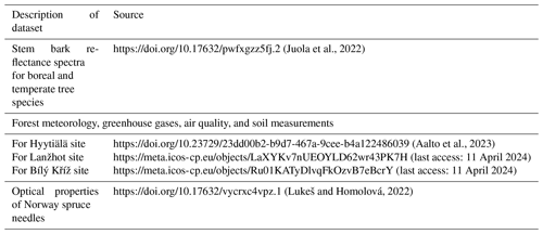
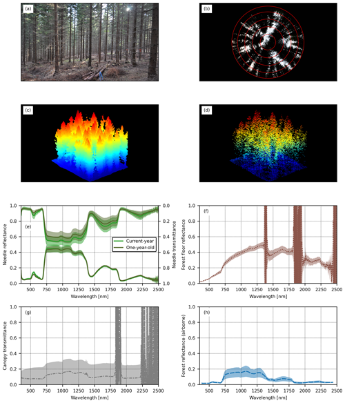
Figure 3 A collection of figures summarizing the different types of data collected for a pure coniferous plot located in Bílý Kříž (stand ID “BK_SPRUCE2” in the dataset). The dominant tree species is Norway spruce (99 % of basal area), with an effective plant area index of 2.8 and a mean tree height of 20.8 m. (a) An overview photograph of the plot (from the northeastern corner towards the plot center). (b) A hemispherical photograph of the canopy (Sect. 2.3.3). (c) Point cloud visualization of the plot based on terrestrial laser scanning data from the south-west corner towards the plot center based on a downsampled point cloud (Sect. 2.3.2). (d) Point cloud visualization of the plot based on airborne laser scanning data from the southwestern corner towards the plot center (from view zenith angle 45°, 17 pulses m⁻²) (Sect. 2.4.2). (e) Mean leaf-level reflectance and transmittance spectra (DHRF and DHTF, respectively) and their standard deviations for current-year and 1-year-old needles of the dominant tree species in the plot (Sect. 2.3.6). (f) Mean reflectance spectrum (HCRF) and its standard deviation for the forest floor in the plot (Sect. 2.3.4). Spectral regions with noise were caused by atmospheric water vapor. (g) Mean spectral transmittance and its standard deviation for the tree canopy layer (Sect. 2.3.5). Spectral regions with noise were mainly caused by atmospheric water vapor but also by the reduced sensitivity of the cosine receptor at the end of the spectral range (>2200 nm). (h) Mean reflectance spectrum (HDRF) and its standard deviation for the entire plot (25 m × 25 m area) based on airborne measurements (Sect. 2.4.1).

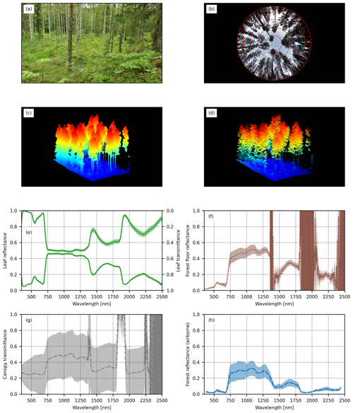
Figure 4 A collection of figures summarizing the different types of data collected for a broadleaved plot located in Hyytiälä (stand ID “HY_BIRCH2” in the dataset). The dominant tree species is silver birch (85 % of basal area), with an effective plant area index 1.5 of and a mean tree height of 23.2 m. (a) An overview photograph of the plot (from the northwestern corner towards the plot center). (b) A hemispherical photograph of the canopy (Sect. 2.3.3). (c) Point cloud visualization of the plot based on terrestrial laser scanning data from the southwestern corner towards the plot center based on a downsampled point cloud (Sect. 2.3.2). (d) Point cloud visualization of the plot based on airborne laser scanning data from the southwestern corner towards the plot center (from view zenith angle 45°, 48 pulses m⁻²) (Sect. 2.4.2). (e) Mean leaf-level reflectance and transmittance spectra (DHRF and DHTF, respectively) and their standard deviations for the dominant tree species in the plot (Sect. 2.3.6). (f) Mean reflectance spectrum (HCRF) and its standard deviation for the forest floor in the plot (Sect. 2.3.4). Spectral regions with noise were caused by atmospheric water vapor. (g) Mean spectral transmittance and its standard deviation for the tree canopy layer (Sect. 2.3.5). Spectral regions with noise were mainly caused by atmospheric water vapor but also by the reduced sensitivity of the cosine receptor at the end of the spectral range (>2200 nm). (h) Mean reflectance spectrum (HDRF) and its standard deviation for the entire plot (25 m × 25 m area) based on airborne measurements (Sect. 2.4.1).

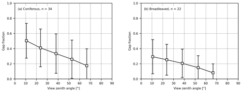
Figure 5 Mean and standard deviation of canopy gap fractions in concentric view zenith angles as obtained from hemispherical photographs in (a) coniferous and (b) broadleaved forests. Here, coniferous and broadleaved forests were defined so that at least 75 % of the trees (based on basal area) within the plot were coniferous or broadleaved species, respectively. The data shown in this figure are based on measurements described in Sect. 2.2.3 (n= number of plots).

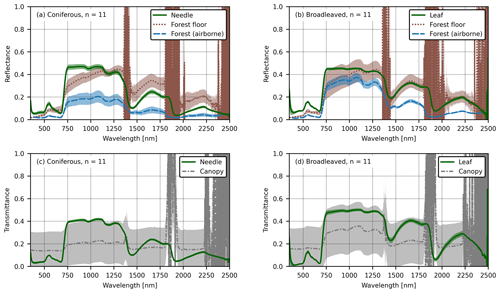
Figure 6 Mean spectra at different scales. (a) Mean reflectance spectra and their standard deviations for needles, the forest floor, and the entire forest plot in coniferous forests. (b) Mean reflectance spectra and their standard deviations for leaves, the forest floor, and the entire forest plot in broadleaved forests. (c) Mean transmittance spectra and their standard deviations for needles and canopies in coniferous forests. (d) Mean transmittance spectra and their standard deviations for needles and canopies in broadleaved forests. The data shown in this figure are based on measurements and reflectance quantities described and defined in Sect. 2.2.4–2.2.6 and 2.4.1., and only the subset of plots which had measurements of canopy transmittance are included here. Coniferous and broadleaved forests were defined so that at least 75 % of the trees (based on basal area) within the plot were coniferous or broadleaved species, respectively. For visualization purposes, leaf-level reflectance and transmittance spectra were first computed at the plot level as averages weighted by tree species proportions and needle age classes and then were averaged over all plots to obtain the mean and standard deviation values shown in the above. Forest floor reflectance and canopy transmittance data are shown with the noise that is inherently present in atmospheric water absorption bands in spectral data measured outdoors. Forest reflectance (HDRF at plot level, panels (a) and (b)) is averaged for an area of 25 m × 25 m in each stand and is based on airborne CASI and SASI data (n refers to the number of plots).

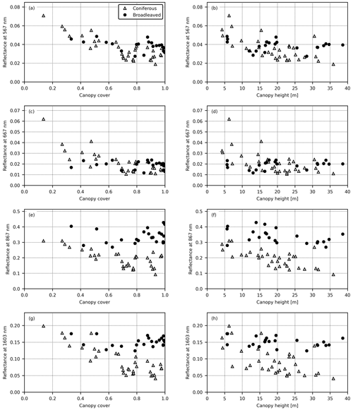
Figure 7 The relationship between forest reflectance (HDRF, obtained from airborne CASI and SASI data) and forest structure (obtained from ALS data, scan zenith angle max 20°) for broadleaved and coniferous forests in four spectral regions: green (567 nm), red (667 nm), near-infrared (NIR, 867 nm), and shortwave infrared (SWIR, 1603 nm). The data are averaged for an area of 25 m × 25 m in each stand. Canopy cover was defined as the first echo cover index in ALS data so that the first echoes originating from the canopy were divided by all the first echoes in the plot. (a, c, e, g) Canopy cover and forest reflectance (HDRF). Spectral region indicated on the y axis. (b, d, f, h) Canopy height (defined as the 95th percentile of all canopy echoes in ALS data) and forest reflectance (HDRF). Spectral region indicated on the y axis. Coniferous and broadleaved forests were defined so that at least 75 % of the trees (based on basal area) within the plot were coniferous or broadleaved species, respectively. The data shown in this figure are based on measurements described in Sect. 2.4.

2.5 External field datasets

Field datasets from other sources and which are relevant to physically based remote sensing but not included in our campaigns are available for the study sites. We have summarized these datasets in Table 2. They include (1) reflectance spectra of tree bark for boreal and temperate tree species; (2) additional datasets on the optical properties of Norway spruce needles from the Czech study sites; and (3) forest meteorology, greenhouse gases, air quality, and soil measurements from ICOS towers.

3 Results

The data allow a comprehensive examination of the spectral and structural properties of forest stands. We summarized the different data sources in two sets of figures using a coniferous stand from Bílý Kříž (Fig. 3) and a broadleaved stand from Hyytiälä (Fig. 4) as examples. These two forest stands illustrate the variation in structural and spectral properties both within and between stands present in the new dataset. For example, the point clouds produced by laser scanning sensors and described in this paper (Figs. 3c–d and 4c–d) can be used to visualize and compute canopy height distribution or density metrics or to assess the spatial distribution patterns of trees or foliage clumping in the study stands. The variation in the spectral properties of the study stands, on the other hand, can be divided into several parts to examine tree leaf-level (Figs. 3e, 4e), forest-floor-level (Figs. 3f, 4f), and tree canopy-level (Figs. 3g–h, 4g–h) phenomena. As a specific example of a key structural variable needed in RT modeling of vegetation, we publish data on tree canopy gap fractions at different view angles based on hemispherical photography. On average, in our coniferous stands, canopy gap fractions were approximately 2 times as high as in the broadleaved stands, and in both types of forests, the gap fractions decreased linearly towards the horizon (Fig. 5).

Using the datasets described in this paper, differences in the spectral properties of forests can be investigated at multiple scales (Fig. 6). In presenting the data here, we refer to the spectral regions as visible (∼400–700 nm), near infrared (∼700–1300 nm), and shortwave infrared (∼1300–2500 nm). In both coniferous and broadleaved stands, the reflectances were notably higher at the tree leaf level than at the stand (canopy) level throughout the entire measured spectrum (Fig. 6a–b). Forest floor reflectances, on the other hand, were usually lower than tree leaf-level reflectances but were higher than canopy-level reflectances in the visible and near-infrared regions. However, in the shortwave-infrared region, the forest floor had, on average, a higher reflectance than tree leaves or canopies in coniferous stands and a reflectance similar to that of tree leaves in broadleaved stands (Fig. 6a–b). An especially unique feature of this dataset is that transmittance spectra at leaf and canopy levels were also measured so that they could be used in, for example, testing the performance of RT models. In our data, the canopy-level spectral transmittance of coniferous stands was more stable throughout the spectrum than the canopy-level transmittance of broadleaved stands, and transmittances at the leaf and canopy levels were usually lower in our coniferous study plots than in broadleaved study plots (Fig. 6c–d). Furthermore, the data show that, in the visible region, the spectral transmittance at the canopy level was higher than the spectral transmittance at leaf level. In the near-infrared and shortwave-infrared regions, on the other hand, leaf-level transmittances were higher than canopy-level transmittances. An exception to this was in the coniferous stands in two spectral regions – around 1400–1500 nm and above ∼1900 nm – where canopy-level transmittances were, again, higher than leaf-level transmittances. In broadleaved stands, the canopy spectral transmittances in the shortwave-infrared range were higher than leaf-level transmittances only in a small region around 1900–2000 nm.

Finally, the data also allow for an examination of the relationships between structural and spectral properties of forests through a combination of contemporaneous airborne laser scanning and hyperspectral data (Fig. 7). These data can be used to illustrate, for example, that, in the visible spectral region, forest reflectance decreased as a function of increasing canopy cover (defined as the first echo cover index in ALS data) across forest stands representing different biomes (Fig. 7a, c) but that, in the near-infrared and shortwave-infrared regions, broadleaved and coniferous stands with closed canopies (i.e., high canopy cover values) formed two distinct groups so that coniferous stands had notably lower HDRFs than broadleaved stands did (Fig. 7e, g). Similar phenomena were also observed in the relationships between forest reflectance and canopy height (defined as the 95th percentile of all canopy echoes) obtained from ALS data (Fig. 7b, d, f, h).

4 Data availability

The data are available in the open-access repository Fairdata IDA, which is a research data storage service provided by the Ministry of Education and Culture of Finland. The data can be accessed at Hovi et al. (2024a, https://doi.org/10.23729/9a8d90cd-73e2-438d-9230-94e10e61adc9) (for data described in Section 2.3.) and Hovi et al. (2024b, https://doi.org/10.23729/c6da63dd-f527-4ec9-8401-57c14f77d19f) (for data described in Sect. 2.4).

5 Conclusions

Radiative transfer models of vegetation play a key role in advancing remote sensing science. The development of these models has been hindered by a lack of comprehensive ground reference data on both the structural and spectral characteristics of forests. In this paper, we introduced datasets containing information on the structural and spectral properties of temperate, hemiboreal, and boreal European forest stands. We anticipate that these data will have wide use in testing and validating radiative transfer models for forests and in other remote sensing studies beyond radiative transfer model development.

Appendix A

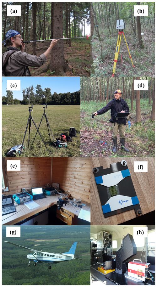
Figure A1 Photographs of different types of measurements conducted during the campaigns. (a) Forest inventory measurements. (b) Terrestrial laser scanning (TLS). (c) Spectral transmittance reference measurements in an open place. (d) Forest floor spectral measurements. (e) Laboratory measurements of the spectral properties of foliage. (f) Needle carriers used in the spectral measurements of foliage. (g) Cessna 208B Grand Caravan aircraft used in the airborne campaigns. (h) View of the sensors inside the Cessna aircraft.

Figure A2 Schemata showing the illumination and view geometries during the collection of field and laboratory data (Sect. 2.3).