Gridded dataset of nitrogen and phosphorus point sources from wastewater in Germany (1950–2019)

Knowledge about the long history of the anthropogenic inputs of nitrogen (N) and phosphorus (P) is crucial to capture long-term N and P processes (legacies) and to investigate water quality and ecosystem health. These inputs include N and P point sources, which mainly originate from wastewater and which are directly discharged into surface waters, thus having an immediate impact on ecosystem functioning. However, N and P point sources are challenging to estimate, due to the scarcity of and uncertainty in observational data. Here, we contribute towards improved characterisation of N and P point sources from wastewater by providing a long-term (1950–2019), high-resolution (0.015625° ≈1.4 km on average) dataset for Germany. The dataset includes both domestic and industrial emissions treated in wastewater treatment plants and untreated domestic emissions that are collected in the sewer system. We adopt a modelling approach that relies on a large range of data collected from different sources. Importantly, we account for the uncertainties arising from different modelling choices (i.e. coefficients and downscaling approach). We provide 200 gridded N and P point source realisations, which are constrained and evaluated using available (recent) observations of wastewater treatment plants' outgoing loads. We discuss the uncertainties in our reconstructed dataset over a large sample of river basins in Germany and provide guidance for future uses. Overall, by capturing the long-term spatial and temporal variations in N and P point sources and accounting for uncertainties, our dataset can facilitate long-term and large-scale robust water quality studies. The dataset is available at https://doi.org/10.5281/zenodo.10500535 (Sarrazin et al., 2024).

1 Introduction

Anthropogenic nitrogen (N) and phosphorus (P) enrichment in fresh and marine waters has been observed worldwide, with adverse effects on both human health and ecosystem health (Millenium Ecosystem Assessment, 2005). Specifically, this N and P excess can induce eutrophication of water bodies, resulting first in the excessive development of primary producers, such as phytoplankton and algae that can themselves be toxic to aquatic species and humans, and second in a reduction in dissolved oxygen levels (hypoxia) that can impair aquatic ecosystems (Conley et al., 2009; Dodds and Smith, 2016; Lemley and Adams, 2019; Smith, 2003). In the most severe cases, a (almost) complete oxygen depletion can occur (anoxia), leading to the appearance of periodic or persistent “dead zones” that are unsuitable to sustain most (aquatic) lives (Diaz and Rosenberg, 2008). Further, inorganic N compounds also cause the acidification of water bodies, are toxic to aquatic species, and make water supply unsafe to drink (Camargo and Alonso, 2006; Lin et al., 2023; WHO, 2016). Notably, not only N and P excess but also changes in the relative proportions of N and P compared to natural conditions have negative consequences on the structure, functioning, and diversity of (aquatic) ecosystems (Penuelas et al., 2013, 2020).

N and P contamination of water bodies is a long-standing problem that has developed since the beginning of the twentieth century and more intensively since the mid-twentieth century, due to an increase in anthropogenic N and P sources (Selman et al., 2008; Le Moal et al., 2019). Importantly, N and P inputs to the environment can affect the water quality status over decades because of the long timescales of the hydrologic transport and biogeochemical and erosional processes controlling the discharge of nutrients to aquatic systems and the nutrient turnover within aquatic systems. Previous studies have shown that an accumulation (legacy) of N can occur in the soil (Jenkinson, 1991; Sebilo et al., 2013; Van Meter et al., 2016), vadose zone (Ascott et al., 2017; Wang et al., 2012), and groundwater (Puckett et al., 2011; Stuart et al., 2007) and of P in the soil (Parkhurst et al., 2022; Pavinato et al., 2020; Zhang et al., 2022) and in the sediments in rivers (Sharpley et al., 2013), lakes (O'Connell et al., 2020), and marine environments (Gustafsson et al., 2012; Herbert and Fourqurean, 2008; Kuliński et al., 2022). These N and P legacies can induce a delay between reductions in anthropogenic N and P sources and the corresponding response of water quality (Basu et al., 2022; Ehrhardt et al., 2019; Grimvall et al., 2000; Sharpley et al., 2013; Vero et al., 2018), eutrophication, and hypoxia (Gustafsson et al., 2012; Kemp et al., 2009), as well as the response of aquatic ecosystems in terms of species abundance, biodiversity, and functions (Jones et al., 2018; McCrackin et al., 2017). In addition, ecosystem recovery from anthropogenic disturbance, such as eutrophication, is a slow process that can take decades or even longer, depending on the intensity and duration of the disturbance (Duarte et al., 2020; McCrackin et al., 2017; Moreno-Mateos et al., 2017, 2020).

To support nutrient management strategies, a quantification of long-term past sources of both N and P is crucial to drive water quality models over long timescales (decades to centuries) and thus to elucidate the temporal developments of water quality and nutrient legacies (e.g. Lee et al., 2016; Mittelstet and Storm, 2016; Van Meter et al., 2017, 2021). This is also needed to force water quality models over the period with output observations (such as N and P in-stream concentrations), thus allowing for model calibration and evaluation (Sarrazin et al., 2022). N and P sources are separated into two categories, namely point and diffuse sources. Point sources correspond to “a stationary location or fixed facility from which pollutants are discharged; any single identifiable source of pollution” (EEA, 2023c). They encompass domestic, industrial, and commercial wastewater that may or may not undergo treatment in wastewater treatment plants (WWTPs), urban runoff that is collected in sewers, and intensive livestock operations and fish farms (EEA, 2005; Macias Moy et al., 2022; OECD, 2017). Diffuse sources are “without a single point of origin or not introduced into a receiving stream from a specific outlet” (EEA, 2023c). They include N and P mineral fertilisers and manure application to soils, N and P atmospheric deposition, N biological fixation, P release through weathering, wastewater from households not connected to the sewer system nor to WWTPs, and additional sources in (impervious) urban areas (leaf fall and animal excrement) (Batool et al., 2022; Byrnes et al., 2020; Fuchs et al., 2010; Macias Moy et al., 2022). Both point and diffuse sources are important contributors to N and P levels in receiving water bodies (e.g. Bouraoui et al., 2011; Sarrazin et al., 2022). The focus of this study is on point sources.

The estimation of long-term N and P point sources from wastewater is challenging, as direct measurements are scarce and uncertain. In Europe, the European Union (EU) only makes observations for the recent period available, namely N and P loads from urban WWTPs and so-called “direct” industrial release. First, within the frame of the European Urban Waste Water Treatment Directive (EC, 1991), the EU has published N and P loads for urban WWTPs from 2010 onward, including both domestic emissions and so-called “indirect” industrial emissions that are treated in urban WWTPs (Waterbase; EEA, 2023b). Second, within the frame of the European Pollutant Release and Transfer Register Regulation (E-PRTR; EC, 2006) and the Industrial Emissions Directive (IED; EC, 2010), the EU has provided, from 2007 onward, direct industrial N and P release to water (without treatment in urban WWTPs), as well as emissions from the largest urban WWTPs (EEA, 2020, 2023a). However, these observational datasets are not exhaustive. On the one hand, E-PRTR and IED data records may greatly underestimate industrial emissions to water, since they only cover large industrial activities. They also only include emissions above some prescribed threshold levels, which correspond to a small fraction of facilities subject to reporting (e.g. around 10 % in 2016 in E-PRTR), as discussed in EEA (2019). On the other hand, load data in the Waterbase dataset (EEA, 2023b) are only reported for some WWTPs included in the record (Vigiak et al., 2020). Moreover, the Waterbase dataset only contains records for larger WWTPs treating wastewater from agglomerations with more than 2000 population equivalent (PE; one PE being defined as the organic biodegradable load having a 5 d biochemical oxygen demand (BOD5) of 60 g of oxygen per day, EC, 1991). Knowledge about the N and P discharge from smaller WWTPs is, however, crucial to understand the water quality in smaller order streams (Yang et al., 2019b, a).

Given this data limitation, modelling strategies are typically used to quantify past N and P point sources. In this respect, on a global scale, Morée et al. (2013) assessed N and P point sources from wastewater for the period 1900–2000. Their approach, which builds on the study of Van Drecht et al. (2009), is based on data at the country level and proxy data when more precise data could not be collected (such as data of gross domestic product that are used to estimate P detergent). On a European scale, Vigiak et al. (2020, 2023) provide N and P point sources from wastewater at river basin scale (CCM2 catchments; Jager and Vogt, 2007) for the period 1990–2016. For this, they used the WWTP data of Waterbase for the recent years (2014 and 2016) for EU countries and a methodology similar to that of Morée et al. (2013) for the period 1990–2010 (further details in Grizzetti et al., 2022; Vigiak et al., 2020). These approaches to past data reconstruction that rely on country-level statistics are useful for large-scale water quality assessment. However, they do not account for the sub-national variability that can be large for countries such as Germany, which was divided between a western and an eastern part between 1949 and 1990. Specifically, the performance of the wastewater handling system in East Germany was lagging behind that of West Germany before German reunification in 1990 and in the following years, whereby efforts were put in place to improve wastewater treatment in East Germany (Rudolph and Block, 2001) (all uses of “East” and “West” Germany in the current paper are referring to the former officially defined regions). In Germany, N and P point source data are only provided by the German Environmental Agency at country level for the period 1987–2016 (UBA, 2020). The methodology, which is described in multiple reports for the different years (Behrendt et al., 2000; Fuchs et al., 2010, 2017, 2022), is based on confidential microdata at the WWTP level, as well as on data on industrial direct emissions, in particular from the E-PRTR dataset. Modelling assumptions compensate for the paucity of data for the past period, where in particular WWTP microdata were lacking, as documented for the year 1985 and 1995 in Behrendt et al. (2000). Importantly, despite the large uncertainties in the point source data arising from data scarcity and uncertainty, and modelling assumptions, uncertainties were not accounted for in the data of Vigiak et al. (2020, 2023) and UBA (2020).

Our review of the literature reveals the need for a long-term dataset of past N and P point sources to support water quality assessment over Germany that accounts for the spatial differences within Germany as well as uncertainties. This is crucial to inform water quality strategies in Germany, where the majority of the national monitoring sites for flowing surface water have shown nitrate and phosphorus concentrations above a limit that would ensure a good ecological status (for instance, 81 % for nitrate and 70 % for phosphorus in 2015; Arle et al., 2017). Furthermore, N and P emissions in Germany have contributed to the eutrophication of the North and Baltic Sea since the mid-twentieth century (EEA et al., 2019; Arle et al., 2017). To address this gap, here we present consistent N and P point source estimates from wastewater over a 0.015625° resolution grid (around 1.4 km) in Germany for the period 1950–2019. We account for the uncertainties arising from different modelling choices, namely coefficients and spatial disaggregation approaches to construct grid-level information based on state-level estimates derived for the 16 German federal states. Our state-level (in EU classification “Nomenclature of Territorial units for statistics” level 1 – NUTS-1) estimates are based on state-level (NUTS-1) statistical data, which we compile from different sources, or country-level (NUTS-0) statistics in the absence of finer-resolution data. We use a modelling approach that builds in particular on Morée et al. (2013), Van Drecht et al. (2009), Vigiak et al. (2020), and IPCC (2019), while we make use of observational data of WWTP N and P emissions to constrain our modelled estimates and check their plausibility. As in previous studies (Morée et al., 2013; Van Drecht et al., 2009; UBA, 2020; Vigiak et al., 2020, 2023), we assess total N and P without distinction between the different forms of N and P. Our dataset encompasses emissions treated in urban WWTPs, including domestic and industrial (indirect) emissions, as well as untreated domestic emissions collected in the sewer system. It contributes towards better characterisation of wastewater emissions and their impact on the surrounding (aquatic) environment. In this paper, we discuss the uncertainties of our point source estimates at grid and river basin level to guide future uses of the dataset for water quality studies.

2 N and P point source model

We estimate N and P gross emissions to wastewater and point sources to surface water (net emissions), building on the studies of Morée et al. (2013), Van Drecht et al. (2009), and Vigiak et al. (2020), as well as IPCC (2019) for N emissions only. We consider both domestic and industrial (commercial) indirect emissions that are collected in the sewer system and/or treated in WWTPs. Our approach, which is summarised in Fig. 1, uses 18 parameters (or coefficients) defined in Table 1. We first estimate the total N and P point source emissions as well as their partitioning over urban and rural areas at NUTS-1 level (Sect. 2.1). These NUTS-1 level data are then subsequently downscaled to grid level (Sect. 2.2).

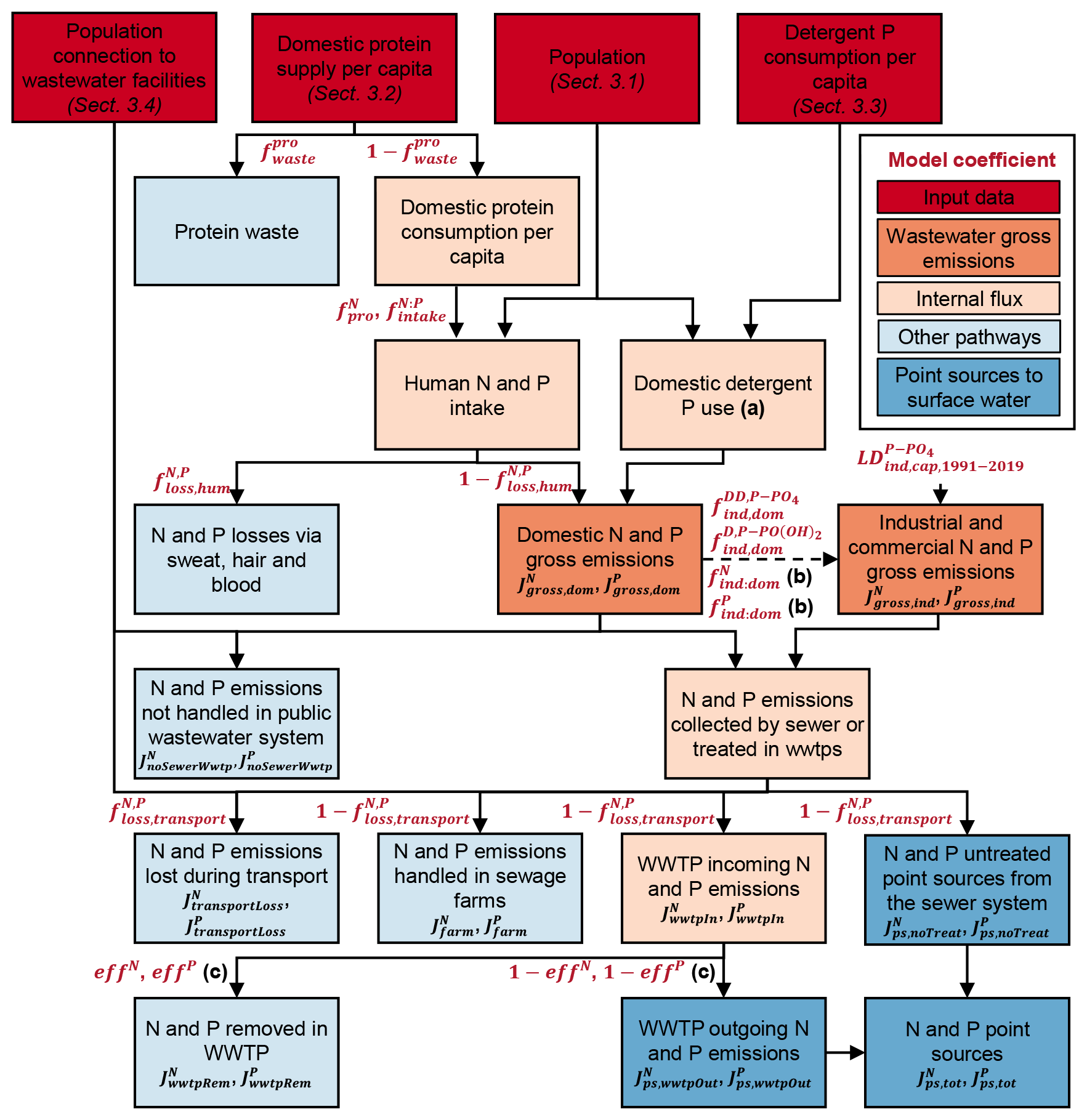
Figure 1 Schematic representation of the N and P point source model, including the model coefficients (defined in Table 1), the model input data (described in Sect. 3.1–3.4), and the model fluxes. The fluxes comprise the N and P wastewater domestic and industrial and commercial gross emissions; the model internal N and P fluxes; the N and P point sources to surface water and their two components, that is the treated emissions coming from WWTPs and the untreated emissions coming from the sewer system; and other pathways. We note that (a) the laundry detergent phosphate data we use include both the domestic and the industrial and commercial components before 1990 (Sect. 3.3.1); (b) the fractions of industrial and commercial to domestic gross N and P emissions, denoted as $f_{\mathrm{ind}:\mathrm{dom}}^{\mathrm{N}}$ and $f_{\mathrm{ind}:\mathrm{dom}}^{\mathrm{P}}$, respectively, are estimated from values in 1950 and 2000, which are defined as model coefficients (see Table 1); and (c) the efficiency of N and P removal, denoted as eff^N and eff^P, respectively, results from the combination of the efficiencies of removal for the different treatment types (defined in Table 1).

Table 1 Description of the model parameters and ranges used in this study.

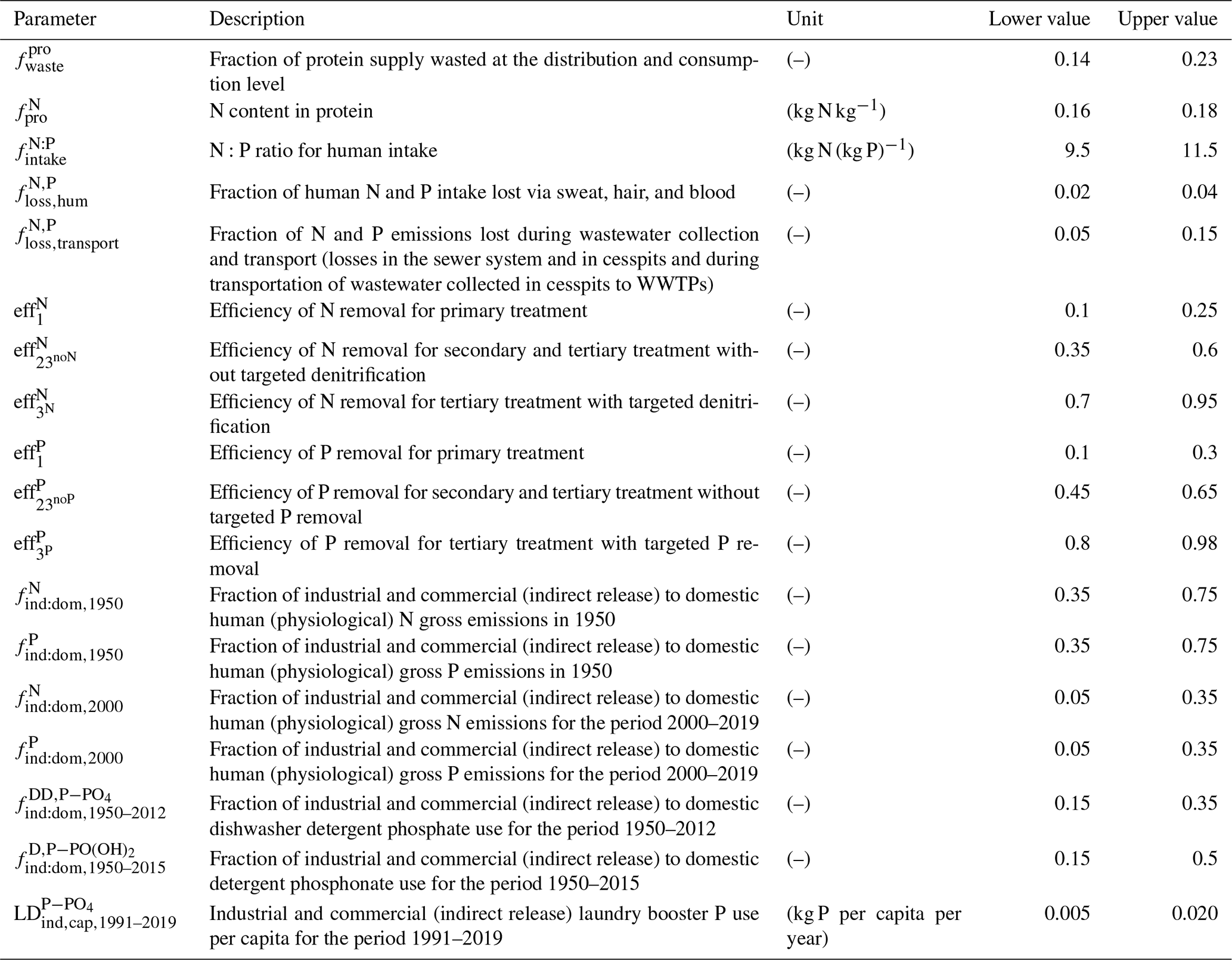
Note that explanations and references for the determination of the ranges are reported in Table S2 in the Supplement. The parameters are sampled from a uniform distribution.

N and P gross emissions to wastewater can follow other pathways than point sources to surface water; these are depicted in light-blue colour in Fig. 1. First, some of the N and P gross emissions are not handled in the public wastewater system; that is, they are not collected in the sewer system nor treated in WWTPs. Second, some of the emissions that are collected in the sewer system or treated in WWTPs are lost during collection and transportation (e.g. sewer losses). Third, some of the emissions that are collected in the sewer system can be applied to agricultural soils in sewage farms and are thus a diffuse source to surface water. Fourth, through treatment in WWTPs, some of the N and P emissions are removed from the wastewater according to the efficiency of N and P removal. Further details on these pathways and their quantitative estimation are reported in Sect S2 in the Supplement.

2.1 N and P emissions at NUTS-1 level

2.1.1 Domestic and industrial N and P gross emissions

Following IPCC (2019) and Morée et al. (2013), we estimate domestic human (physiological) N gross emissions to wastewater per capita, which correspond to the amount of N in human excreta, as a function of the protein supply per capita at the distribution level Pro${}_{\mathrm{supply},\mathrm{cap}}(t,i)$ (kg per capita per year); the fraction of protein supply wasted at the distribution and consumption level $f_{\mathrm{waste}}^{\mathrm{pro}}$ (–); the N content in protein $f_{\mathrm{pro}}^{\mathrm{N}}$ (–); and the fraction of human N intake lost via sweat, hair, and blood $f_{\mathrm{loss},\mathrm{hum}}^{\mathrm{N},\mathrm{P}}$ (–). We derive the total as well as the urban and rural N gross emissions at time t and for the ith NUTS-1 region denoted as $J_{\mathrm{gross},\mathrm{dom},X}^{\mathrm{N}}(t,i)$ (kg yr⁻¹) based on the population count Pop_X(t), where X can be urb (urban component), rur (rural component), and all (total, i.e. sum, of urban and rural components):

$$\begin{array}{}\text{(1)}& \begin{array}{rl}{J}_{\mathrm{gross},\mathrm{dom},X}^{\mathrm{N}}(t,i)& ={\mathrm{Pop}}_X(t,i){\mathrm{Pro}}_{\mathrm{supply},\mathrm{cap}}(t,i)f_{\mathrm{pro}}^{\mathrm{N}}\\ & \times (\mathrm{1}-f_{\mathrm{waste}}^{\mathrm{pro}})(\mathrm{1}-f_{\mathrm{loss},\mathrm{hum}}^{\mathrm{N},\mathrm{P}}).\end{array}\end{array}$$

The level of domestic P gross emissions $J_{\mathrm{gross},\mathrm{dom},X}^{\mathrm{P}}(t,i)$ (kg yr⁻¹) is estimated assuming a constant N:P ratio for human intake $f_{\mathrm{intake}}^{\mathrm{N}:\mathrm{P}}$ (kg N (kg P)⁻¹) (Morée et al., 2013) and considering P emissions from the use of detergents:

$$\begin{array}{}\text{(2)}& \begin{array}{rl}{J}_{\mathrm{gross},\mathrm{dom},X}^{\mathrm{P}}(t,i)& ={\displaystyle \frac{J_{\mathrm{gross},\mathrm{dom},X}^{\mathrm{N}}(t,i)}{f_{\mathrm{intake}}^{\mathrm{N}:\mathrm{P}}}}+{\mathrm{Pop}}_X(t,i)\\ & \times \left({\mathrm{LD}}_{\mathrm{dom},\mathrm{cap}}^{\mathrm{P}-{\mathrm{PO}}_{\mathrm{4}}}(t,i)+{\mathrm{DD}}_{\mathrm{dom},\mathrm{cap}}^{\mathrm{P}-{\mathrm{PO}}_{\mathrm{4}}}(t,i)\right.\\ & \left.+D_{\mathrm{dom},\mathrm{cap}}^{\mathrm{P}-\mathrm{PO}(\mathrm{OH}{)}_{\mathrm{2}}}(t,i)\right),\end{array}\end{array}$$

where LD${}_{\mathrm{dom},\mathrm{cap}}^{\mathrm{P}-{\mathrm{PO}}_{\mathrm{4}}}(t,i)$ (kg P per capita per year) is the domestic laundry detergent phosphate P use per capita, DD${}_{\mathrm{dom},\mathrm{cap}}^{\mathrm{P}-{\mathrm{PO}}_{\mathrm{4}}}(t,i)$ (kg P per capita per year) is the domestic dishwasher detergent phosphate P use per capita, and $D_{\mathrm{dom},\mathrm{cap}}^{\mathrm{P}-\mathrm{PO}(\mathrm{OH}{)}_{\mathrm{2}}}(t,i)$ (kg P per capita per year) is the domestic detergent phosphonate P use per capita. We note that LD${}_{\mathrm{dom},\mathrm{cap}}^{\mathrm{P}-{\mathrm{PO}}_{\mathrm{4}}}(t,i)$ includes both domestic and industrial and commercial use until the year 1991 and 1992 for West Germany and East Germany, respectively, as the available data do not allow these two parts to be separated (Sect. 3.3.1). While Morée et al. (2013) and Van Drecht et al. (2009) rely on a modelling approach using proxy data such as gross domestic product (GDP) to reconstruct P emissions from detergents, our estimation is based on detergent data that we collect for Germany (Sect. 3.3).

We assess industrial and commercial gross emissions as a fraction of total human emissions following previous studies (IPCC, 2019; Morée et al., 2013; Vigiak et al., 2020). We consider a time-varying fraction of industrial and commercial to domestic gross N and P emissions ($f_{\mathrm{ind}:\mathrm{dom}}^{\mathrm{N}}(t,i)$ (–), $f_{\mathrm{ind}:\mathrm{dom}}^{\mathrm{P}}(t,i)$ (–), respectively) that decreases linearly between 1950 and 2000, similar to Morée et al. (2013), and that remains constant after 2000 as follows:

• When t≤2000,

  $$\begin{array}{}\text{(3)}& \begin{array}{rl}{f}_{\mathrm{ind}:\mathrm{dom}}^{\mathrm{N}}(t,i)& =f_{\mathrm{ind}:\mathrm{dom},\mathrm{1950}}^{\mathrm{N}}\\ & +{\displaystyle \frac{f_{\mathrm{ind}:\mathrm{dom},\mathrm{2000}}^{\mathrm{N}}-f_{\mathrm{ind}:\mathrm{dom},\mathrm{1950}}^{\mathrm{N}}}{\mathrm{50}}}\\ & \times (t-\mathrm{1950}).\end{array}\end{array}$$

• When t>2000,

  $$\begin{array}{}\text{(4)}& f_{\mathrm{ind}:\mathrm{dom}}^{\mathrm{N}}(t,i)=f_{\mathrm{ind}:\mathrm{dom},\mathrm{2000}}^{\mathrm{N}},\end{array}$$

where $f_{\mathrm{ind}:\mathrm{dom},\mathrm{1950}}^{\mathrm{N}}$ (–) and $f_{\mathrm{ind}:\mathrm{dom},\mathrm{2000}}^{\mathrm{N}}$ (–) are the fractions of industrial and commercial to domestic N gross emissions in 1950 and 2000, respectively. Similar equations are used to assess $f_{\mathrm{ind}:\mathrm{dom}}^{\mathrm{P}}(t,i)$.

To estimate the N and P gross emissions to wastewater, we apply the above coefficients (Eqs. 3–4) to the total human N and P emissions (Eqs. 1–2), while also accounting for the detergent P use in businesses and institutions such as bars, restaurants, canteens, hotels, bakeries, butcher shops, schools, hospitals, and retirement homes (see details on industrial and commercial detergents in Mehlhart et al., 2021). We also consider that industrial and commercial activities are located in urban areas only; hence industrial and commercial rural N and P gross emissions are considered to be equal to zero. The industrial and commercial urban N and P gross emissions, denoted as $J_{\mathrm{gross},\mathrm{ind},\mathrm{urb}}^{\mathrm{N}}(t,i)$ (kg yr⁻¹) and $J_{\mathrm{gross},\mathrm{ind},\mathrm{urb}}^{\mathrm{P}}(t,i)$ (kg yr⁻¹), respectively, are calculated as follows:

$$\begin{array}{}\text{(5)}& {\displaystyle }{J}_{\mathrm{gross},\mathrm{ind},\mathrm{urb}}^{\mathrm{N}}(t,i)=f_{\mathrm{ind}:\mathrm{dom}}^{\mathrm{N}}(t,i)J_{\mathrm{gross},\mathrm{dom},\mathrm{all}}^{\mathrm{N}}(t,i),\text{(6)}& {\displaystyle }\begin{array}{rl}{J}_{\mathrm{gross},\mathrm{ind},\mathrm{urb}}^{\mathrm{P}}(t,i)=& {\displaystyle \frac{f_{\mathrm{ind}:\mathrm{dom}}^{\mathrm{P}}(t,i)}{f_{\mathrm{intake}}^{\mathrm{N}:\mathrm{P}}}}{J}_{\mathrm{gross},\mathrm{dom},\mathrm{all}}^{\mathrm{N}}(t,i)+\\ & {\mathrm{Pop}}_{\mathrm{all}}(t,i)\left({\mathrm{LD}}_{\mathrm{ind},\mathrm{cap}}^{\mathrm{P}-{\mathrm{PO}}_{\mathrm{4}}}(t,i)\right.\\ & \left.+{\mathrm{DD}}_{\mathrm{ind},\mathrm{cap}}^{\mathrm{P}-{\mathrm{PO}}_{\mathrm{4}}}(t,i)+D_{\mathrm{ind},\mathrm{cap}}^{\mathrm{P}-\mathrm{PO}(\mathrm{OH}{)}_{\mathrm{2}}}(t,i)\right),\end{array}\end{array}$$

where LD${}_{\mathrm{ind},\mathrm{cap}}^{\mathrm{P}-{\mathrm{PO}}_{\mathrm{4}}}(t,i)$ (kg P per capita per year) is the industrial and commercial laundry detergent phosphate P use per capita, DD${}_{\mathrm{ind},\mathrm{cap}}^{\mathrm{P}-{\mathrm{PO}}_{\mathrm{4}}}(t,i)$ (kg P per capita per year) is the industrial and commercial dishwasher detergent phosphate P use per capita, and $D_{\mathrm{ind},\mathrm{cap}}^{\mathrm{P}-\mathrm{PO}(\mathrm{OH}{)}_{\mathrm{2}}}(t,i)$ (kg P per capita per year) is the industrial and commercial detergent phosphonate P use per capita. Due to a lack of data on industrial and commercial detergent use, we estimate these quantities from domestic detergent use and specific parameters using the following equations:

$$\begin{array}{}\text{(7)}& {\displaystyle }\begin{array}{rl}& {\mathrm{LD}}_{\mathrm{ind},\mathrm{cap}}^{\mathrm{P}-{\mathrm{PO}}_{\mathrm{4}}}(t,i)=\mathrm{0}\text{ when }t\le \mathrm{1990}\left(\text{West Germany}\right)\\ & \text{ or }t\le \mathrm{1991}\left(\text{East Germany}\right),\\ & {\mathrm{LD}}_{\mathrm{ind},\mathrm{cap}}^{\mathrm{P}-{\mathrm{PO}}_{\mathrm{4}}}(t,i)={\mathrm{LD}}_{\mathrm{ind},\mathrm{cap},\text{1991–2019}}^{\mathrm{P}-{\mathrm{PO}}_{\mathrm{4}}}\\ & \text{when }t>\mathrm{1990}\left(\text{West Germany}\right)\\ & \text{ or }t>\mathrm{1991}\left(\text{East Germany}\right),\end{array}\text{(8)}& {\displaystyle }\begin{array}{rl}& {\mathrm{DD}}_{\mathrm{ind},\mathrm{cap}}^{\mathrm{P}-{\mathrm{PO}}_{\mathrm{4}}}(t,i)={\mathrm{DD}}_{\mathrm{dom},\mathrm{cap}}^{\mathrm{P}-{\mathrm{PO}}_{\mathrm{4}}}(t,i)f_{\mathrm{ind}:\mathrm{dom},\text{1950–2012}}^{\mathrm{DD},\mathrm{P}-{\mathrm{PO}}_{\mathrm{4}}}\\ & \text{when }t\le \mathrm{2012},\\ & {\mathrm{DD}}_{\mathrm{ind},\mathrm{cap}}^{\mathrm{P}-{\mathrm{PO}}_{\mathrm{4}}}(t,i)={\mathrm{DD}}_{\mathrm{dom},\mathrm{cap}}^{\mathrm{P}-{\mathrm{PO}}_{\mathrm{4}}}(\mathrm{2012},i)f_{\mathrm{ind}:\mathrm{dom},\text{1950–2012}}^{\mathrm{DD},\mathrm{P}-{\mathrm{PO}}_{\mathrm{4}}}\\ & \text{when }t>\mathrm{2012},\end{array}\text{(9)}& {\displaystyle }\begin{array}{rl}& D_{\mathrm{ind},\mathrm{cap}}^{\mathrm{P}-\mathrm{PO}(\mathrm{OH}{)}_{\mathrm{2}}}(t,i)=D_{\mathrm{dom},\mathrm{cap}}^{\mathrm{P}-\mathrm{PO}(\mathrm{OH}{)}_{\mathrm{2}}}(t,i)f_{\mathrm{ind}:\mathrm{dom},\text{1950–2015}}^{\mathrm{D},\mathrm{P}-\mathrm{PO}(\mathrm{OH}{)}_{\mathrm{2}}}\\ & \text{when }t\le \mathrm{2015},\\ & D_{\mathrm{ind},\mathrm{cap}}^{\mathrm{P}-\mathrm{PO}(\mathrm{OH}{)}_{\mathrm{2}}}(t,i)=D_{\mathrm{dom},\mathrm{cap}}^{\mathrm{P}-\mathrm{PO}(\mathrm{OH}{)}_{\mathrm{2}}}(\mathrm{2015},i)f_{\mathrm{ind}:\mathrm{dom},\text{1950–2015}}^{\mathrm{D},\mathrm{P}-\mathrm{PO}(\mathrm{OH}{)}_{\mathrm{2}}}\\ & \text{when }t>\mathrm{2015},\end{array}\end{array}$$

where LD${}_{\mathrm{ind},\mathrm{cap},\text{1991–2019}}^{\mathrm{P}-{\mathrm{PO}}_{\mathrm{4}}}$ (kg P per capita per year) is the industrial and commercial laundry phosphate P use per capita for the period 1991–2019, $f_{\mathrm{ind}:\mathrm{dom},\text{1950–2012}}^{\mathrm{DD},\mathrm{P}-{\mathrm{PO}}_{\mathrm{4}}}$ (–) is the fraction of industrial and commercial to domestic dishwasher detergent phosphate use for the period 1950–2012, and $f_{\mathrm{ind}:\mathrm{dom},\text{1950–2015}}^{\mathrm{D},\mathrm{P}-\mathrm{PO}(\mathrm{OH}{)}_{\mathrm{2}}}$ (–) is the fraction of industrial and commercial to domestic detergent phosphonate use for the period 1950–2015. Equation (7) accounts for the fact that our data of laundry detergent phosphate include both the domestic and industrial and commercial components until the year 1990 and 1991 for the NUTS-1 regions of West Germany and East Germany, respectively (Eq. 2). In Eqs. (8) and (9), we consider the European Union Detergent Regulation (EC, 2012) that led to a reduction in dishwasher detergent phosphate use and a consequent increase in phosphonate detergent use for domestic detergent only (DD${}_{\mathrm{dom},\mathrm{cap}}^{\mathrm{P}-{\mathrm{PO}}_{\mathrm{4}}}(t,i)$ and $D_{\mathrm{dom},\mathrm{cap}}^{\mathrm{P}-\mathrm{PO}(\mathrm{OH}{)}_{\mathrm{2}}}(t,i)$). These changes occurred after 2012 for DD${}_{\mathrm{dom},\mathrm{cap}}^{\mathrm{P}-{\mathrm{PO}}_{\mathrm{4}}}(t,i)$ and after 2015 for $D_{\mathrm{dom},\mathrm{cap}}^{\mathrm{P}-\mathrm{PO}(\mathrm{OH}{)}_{\mathrm{2}}}(t,i)$ in Germany (Supplement Fig S3). Therefore, we no longer assess DD${}_{\mathrm{ind},\mathrm{cap}}^{\mathrm{P}-{\mathrm{PO}}_{\mathrm{4}}}(t,i)$ and $D_{\mathrm{ind},\mathrm{cap}}^{\mathrm{P}-\mathrm{PO}(\mathrm{OH}{)}_{\mathrm{2}}}(t,i)$ proportionally to the domestic amounts after 2012 and 2015, respectively, but we assume that these two quantities remain constant.

2.1.2 N and P point source emissions from the public wastewater system

Since the equations to calculate the N and P point sources are the same, we denote any of the two nutrients N and P as Nutri. We calculate total, urban, and rural N and P point source (net) emissions coming from the public wastewater system, denoted as $J_{\mathrm{ps},X}^{\mathrm{Nutri}}(t,i)$ (kg yr⁻¹) and defined as

$$\begin{array}{}\text{(10)}& J_{\mathrm{ps},X}^{\mathrm{Nutri}}(t,i)=J_{\mathrm{ps},\mathrm{noTreat},X}^{\mathrm{Nutri}}(t,i)+J_{\mathrm{ps},\mathrm{wwtpOut},X}^{\mathrm{Nutri}}(t,i).\end{array}$$

N and P point sources (Eq. 10) include both the N and P emissions that are collected in the public sewer system but that are not treated (denoted as $J_{\mathrm{ps},\mathrm{noTreat},X}^{\mathrm{Nutri}}(t,i)$ (kg yr⁻¹); see Eqs. 11 and 15) and the N and P emissions that are treated in WWTPs via collection in the public sewer system, as well as in cesspits (sealed tanks) from which the wastewater is transported by trucks to WWTPs (denoted as $J_{\mathrm{ps},\mathrm{wwtpOut},X}^{\mathrm{Nutri}}(t,i)$ (kg yr⁻¹); see Eqs. 13 and 16). We also account for the fraction of emissions lost during wastewater collection and transport through the coefficient $f_{\mathrm{loss},\mathrm{transport}}^{\mathrm{N},\mathrm{P}}$ (–), including losses in the sewer system (Morée et al., 2013) and during transportation of the wastewater collected in cesspits to WWTPs. In the following, we detail the calculation of the urban and rural point sources. The total of the point sources is derived as the sum of the urban and rural components.

Urban point sources

We consider that all industrial and commercial emissions are collected in the sewer system or treated in WWTPs in urban areas and that they are treated following the same efficiencies as the urban domestic emissions. Morée et al. (2013) made a similar assumption but considered the WWTP efficiency for the total domestic emissions (including both urban and rural emissions). We estimate the urban untreated N and P emissions as follows:

$$\begin{array}{}\text{(11)}& \begin{array}{rl}{J}_{\mathrm{ps},\mathrm{noTreat},\mathrm{urb}}^{\mathrm{Nutri}}(t,i)& =\left(\mathrm{1}-f_{\mathrm{loss},\mathrm{transport}}^{\mathrm{N},\mathrm{P}}\right)\\ & \times \left(J_{\mathrm{gross},\mathrm{dom},\mathrm{urb}}^{\mathrm{Nutri}}(t,i)T{\mathrm{0}}_{\mathrm{urb}}(t,i)\right.\\ & \left.+J_{\mathrm{gross},\mathrm{ind},\mathrm{urb}}^{\mathrm{Nutri}}(t,i){\displaystyle \frac{T{\mathrm{0}}_{\mathrm{urb}}(t,i)}{T_{\text{sewer-wwtp,urb}}(t,i)}}\right),\end{array}\end{array}$$

where T0_urb(t,i) (–) is the fraction of urban population connected to the sewer system but not to public wastewater treatment, and T_{sewer-wwtp,urb}(t,i) (–) is the fraction of urban population connected to the sewer system or to WWTPs, which includes the transportation of wastewater from cesspits to WWTPs. $T_{\text{sewer-wwtp},X}(t,i)$ with respect to total (X=all), urban (X=urb), and rural (X=rur) population is estimated as

$$\begin{array}{}\text{(12)}& \begin{array}{rl}{T}_{\text{sewer-wwtp},X}(t,i)& =T{\mathrm{0}}_X(t,i)+T_{\mathrm{farm},X}(t,i)\\ & +T{\mathrm{1}}_X(t,i)+T{\mathrm{23}}_X^{\mathrm{noNutri}}(t,i)\\ & +T{\mathrm{3}}_X^{\mathrm{Nutri}}(t,i),\end{array}\end{array}$$

where T0_X(t,i) (–) is the fraction of population connected to the sewer system but not to public wastewater treatment, TFarm_X(t,i) (–) is the fraction of population connected to sewage farms (see Supplement Sect. S2), T1_X(t,i) (–) is the fraction of population connected to primary (mechanical) treatment, $T{\mathrm{23}}_X^{\mathrm{noNutri}}(t,i)$ (–) is the fraction of population connected to secondary (biological) treatment and tertiary (advanced) treatment without targeted N removal (denitrification, when Nutri=N) and P removal (when Nutri=P), and $T{\mathrm{3}}_X^{\mathrm{Nutri}}(t,i)$ (–) is the fraction of population connected to tertiary treatment with targeted N removal (when Nutri=N) and P removal (when Nutri=P). Not all WWTPs that are equipped with tertiary treatment specifically remove N and P with very high efficiency (further details in the Supplement, Sect. S6 and in particular Fig. S20). In cases without targeted N and P removal, we consider that the efficiency of N and P removal is similar to that of secondary treatment, hence our definition of the treatment classes reported above. To estimate the fraction of both urban and rural population connection to the different types of treatment (Eq. 12) from the data that refer to the total population (see Sect. 3.4), we assume that the wastewater handling system is more advanced in urban areas. Therefore, we consider that the connection of urban population to the more advanced types of treatment has precedence over rural population (see Supplement Sect. S7 for further details).

Treated N and P emissions are assessed based on the fraction of population connected to the different types of treatment and the efficiency of nutrient removal for each treatment type (IPCC, 2019; Morée et al., 2013; Van Drecht et al., 2009). Here, specifically, we estimate the urban N and P treated emissions as

$$\begin{array}{}\text{(13)}& \begin{array}{rl}& J_{\mathrm{ps},\mathrm{wwtpOut},\mathrm{urb}}^{\mathrm{Nutri}}(t,i)=\left(\mathrm{1}-f_{\mathrm{loss},\mathrm{transport}}^{\mathrm{N},\mathrm{P}}\right)\\ & \left(J_{\mathrm{gross},\mathrm{dom},\mathrm{urb}}^{\mathrm{Nutri}}\right(t,i)\left(T{\mathrm{1}}_{\mathrm{urb}}(t,i)(\mathrm{1}-{\mathrm{eff}}_{\mathrm{1}}^{\mathrm{Nutri}})\right.\\ & +T{\mathrm{23}}_{\mathrm{urb}}^{\mathrm{noNutri}}(t,i)(\mathrm{1}-{\mathrm{eff}}_{{\mathrm{23}}^{\mathrm{noNutri}}}^{\mathrm{Nutri}})\\ & \left.+T{\mathrm{3}}_{\mathrm{urb}}^{\mathrm{Nutri}}(t,i)(\mathrm{1}-{\mathrm{eff}}_{{\mathrm{3}}^{\mathrm{Nutri}}}^{\mathrm{Nutri}})\right)+\\ & J_{\mathrm{gross},\mathrm{ind},\mathrm{urb}}^{\mathrm{Nutri}}(t,i){\displaystyle \frac{\begin{array}{c}T{\mathrm{1}}_{\mathrm{urb}}(t,i)(\mathrm{1}-{\mathrm{eff}}_{\mathrm{1}}^{\mathrm{Nutri}})\\ +T{\mathrm{23}}_{\mathrm{urb}}^{\mathrm{noNutri}}(t,i)(\mathrm{1}-{\mathrm{eff}}_{{\mathrm{23}}^{\mathrm{noNutri}}}^{\mathrm{Nutri}})\\ +T{\mathrm{3}}_{\mathrm{urb}}^{\mathrm{Nutri}}(t,i)(\mathrm{1}-{\mathrm{eff}}_{{\mathrm{3}}^{\mathrm{Nutri}}}^{\mathrm{Nutri}})\end{array}}{T_{\text{sewer-wwtp,urb}}(t,i)}}),\end{array}\end{array}$$

where eff${}_{\mathrm{1}}^{\mathrm{Nutri}}$ (–), eff${}_{{\mathrm{23}}^{\mathrm{noNutri}}}^{\mathrm{Nutri}}$ (–), and eff${}_{{\mathrm{3}}^{\mathrm{Nutri}}}^{\mathrm{Nutri}}$ (–) are the efficiencies of N removal (when Nutri=N) and P removal (when Nutri=P) for primary treatment, for secondary and tertiary treatment without targeted N removal (when Nutri=N) and P removal (when Nutri=P), and for tertiary treatment with targeted N removal (when Nutri=N) and P removal (when Nutri=P), respectively. In Eqs. (11) and (13), the fate of the industrial and commercial gross emissions is assessed by normalising the population connection to the different treatment types by T_{sewer-wwtp,urb}(t,i). This ensures that all industrial and commercial gross emissions are collected in the sewer system or treated in WWTPs.

The incoming urban N and P emissions to WWTPs, denoted as $J_{\mathrm{wwtpIn},\mathrm{urb}}^{\mathrm{Nutri}}(t,i)$ (kg yr⁻¹), which do not account for N and P removal in WWTPs, are calculated as

$$\begin{array}{}\text{(14)}& \begin{array}{rl}& J_{\mathrm{wwtpIn},\mathrm{urb}}^{\mathrm{Nutri}}(t,i)=\left(\mathrm{1}-f_{\mathrm{loss},\mathrm{transport}}^{\mathrm{N},\mathrm{P}}\right)\\ & \times \left(J_{\mathrm{gross},\mathrm{dom},\mathrm{urb}}^{\mathrm{Nutri}}\right(t,i\left)\right(T{\mathrm{1}}_{\mathrm{urb}}(t,i)\\ & +T{\mathrm{23}}_{\mathrm{urb}}^{\mathrm{noNutri}}(t,i)+T{\mathrm{3}}_{\mathrm{urb}}^{\mathrm{Nutri}}(t,i))\\ & +J_{\mathrm{gross},\mathrm{ind},\mathrm{urb}}^{\mathrm{Nutri}}(t,i){\displaystyle \frac{\begin{array}{c}T{\mathrm{1}}_{\mathrm{urb}}(t,i)+T{\mathrm{23}}_{\mathrm{urb}}^{\mathrm{noNutri}}(t,i)\\ +T{\mathrm{3}}_{\mathrm{urb}}^{\mathrm{Nutri}}(t,i)\end{array}}{T_{\text{sewer-wwtp,urb}}(t,i)}}).\end{array}\end{array}$$

Rural point sources

In our study, the rural N point sources originate from domestic emissions only and are assessed similar to the domestic components of the urban N point sources (Eqs. 11 and 13). The rural untreated N and P emissions of Eq. (10) are calculated as follows:

$$\begin{array}{}\text{(15)}& \begin{array}{rl}{J}_{\mathrm{ps},\mathrm{noTreat},\mathrm{rur}}^{\mathrm{Nutri}}(t,i)& =\left(\mathrm{1}-f_{\mathrm{loss},\mathrm{transport}}^{\mathrm{N},\mathrm{P}}\right)\\ & \times \left(J_{\mathrm{gross},\mathrm{dom},\mathrm{rur}}^{\mathrm{Nutri}}(t,i)T{\mathrm{0}}_{\mathrm{rur}}(t,i)\right).\end{array}\end{array}$$

The rural treated N and P emissions of Eq. (10) are estimated as

$$\begin{array}{}\text{(16)}& \begin{array}{rl}& J_{\mathrm{ps},\mathrm{wwtpOut},\mathrm{rur}}^{\mathrm{Nutri}}(t,i)=\left(\mathrm{1}-f_{\mathrm{loss},\mathrm{transport}}^{\mathrm{N},\mathrm{P}}\right)\\ & \times J_{\mathrm{gross},\mathrm{dom},\mathrm{rur}}^{\mathrm{Nutri}}(t,i)\left(T{\mathrm{1}}_{\mathrm{rur}}\right(t,i\left)\right(\mathrm{1}-{\mathrm{eff}}_{\mathrm{1}}^{\mathrm{Nutri}})\\ & +T{\mathrm{23}}_{\mathrm{rur}}^{\mathrm{noNutri}}(t,i)(\mathrm{1}-{\mathrm{eff}}_{{\mathrm{23}}^{\mathrm{noNutri}}}^{\mathrm{Nutri}})\\ & +T{\mathrm{3}}_{\mathrm{rur}}^{\mathrm{Nutri}}(t,i)(\mathrm{1}-{\mathrm{eff}}_{{\mathrm{3}}^{\mathrm{Nutri}}}^{\mathrm{Nutri}})).\end{array}\end{array}$$

The incoming rural N emissions to WWTPs, denoted as $J_{\mathrm{wwtpIn},\mathrm{rur}}^{\mathrm{Nutri}}(t,i)$ (kg yr⁻¹), are calculated as

$$\begin{array}{}\text{(17)}& \begin{array}{rl}& J_{\mathrm{wwtpIn},\mathrm{rur}}^{\mathrm{Nutri}}(t,i)=\left(\mathrm{1}-f_{\mathrm{loss},\mathrm{transport}}^{\mathrm{N},\mathrm{P}}\right)J_{\mathrm{gross},\mathrm{dom},\mathrm{rur}}^{\mathrm{Nutri}}(t,i)\\ & \times \left(T{\mathrm{1}}_{\mathrm{rur}}\right(t,i)+T{\mathrm{23}}_{\mathrm{rur}}^{\mathrm{noNutri}}(t,i)+T{\mathrm{3}}_{\mathrm{rur}}^{\mathrm{Nutri}}(t,i\left)\right).\end{array}\end{array}$$

2.2 N and P point source emissions at grid level

We adopt two different approaches to downscale the N and P point source emissions from NUTS-1 level to grid level to account for uncertainty. First, similar to Morée et al. (2013) and Vigiak et al. (2020), we perform the disaggregation according to the population density. We use gridded urban and rural population counts to disaggregate the NUTS-1 level emissions of the ith NUTS-1 region calculated from Eqs. (11), (13), (15), and (16) to the k_ith grid cell that belong to the ith NUTS-1 region, as follows:

$$\begin{array}{}\text{(18)}& {\displaystyle }\begin{array}{rl}& J_{\mathrm{ps},\mathrm{noTreat},\mathrm{grid}}^{\mathrm{Nutri}}(t,k_i)=J_{\mathrm{ps},\mathrm{noTreat},\mathrm{urb}}^{\mathrm{Nutri}}(t,i){\displaystyle \frac{{\mathrm{Pop}}_{\mathrm{urb},\mathrm{grid}}(t,k_i)}{{\mathrm{Pop}}_{\mathrm{urb}}(t,i)}}\\ & +J_{\mathrm{ps},\mathrm{noTreat},\mathrm{rur}}^{\mathrm{Nutri}}(t,i){\displaystyle \frac{{\mathrm{Pop}}_{\mathrm{rur},\mathrm{grid}}(t,k_i)}{{\mathrm{Pop}}_{\mathrm{rur}}(t,i)}}\end{array}\text{(19)}& {\displaystyle }\begin{array}{rl}& J_{\mathrm{ps},\mathrm{wwtpOut},\mathrm{grid}}^{\mathrm{Nutri}}(t,k_i)=J_{\mathrm{ps},\mathrm{wwtpOut},\mathrm{urb}}^{\mathrm{Nutri}}(t,i){\displaystyle \frac{{\mathrm{Pop}}_{\mathrm{urb},\mathrm{grid}}(t,k_i)}{{\mathrm{Pop}}_{\mathrm{urb}}(t,i)}}\\ & +J_{\mathrm{ps},\mathrm{wwtpOut},\mathrm{rur}}^{\mathrm{Nutri}}(t,i){\displaystyle \frac{{\mathrm{Pop}}_{\mathrm{rur},\mathrm{grid}}(t,k_i)}{{\mathrm{Pop}}_{\mathrm{rur}}(t,i)}},\end{array}\end{array}$$

where $J_{\mathrm{ps},\mathrm{noTreat},\mathrm{grid}}^{\mathrm{Nutri}}(t,k_i)$ (kg yr⁻¹) and $J_{\mathrm{ps},\mathrm{wwtpOut},\mathrm{grid}}^{\mathrm{Nutri}}(t,k_i)$ (kg yr⁻¹) are the untreated and treated point source emissions at grid level, respectively; Pop${}_{\mathrm{urb},\mathrm{grid}}(t,k_i)$ and Pop${}_{\mathrm{rur},\mathrm{grid}}(t,k_i)$ are the urban and rural population counts at grid level, respectively; and Pop_urb(t,i) and Pop_rur(t,i) are the urban and rural population counts at NUTS-1 level, respectively.

Second, we use WWTP observations to disaggregate the NUTS-1 level treated emissions of Eqs. (13) and (16). To derive spatially distributed estimates of domestic waste emissions to European waters, Vigiak et al. (2020) also used WWTP data, specifically entering load expressed in population equivalent (PE). In this study, since we have access to detailed WWTP data for Germany, we construct a gridded map of WWTP outgoing N and P loads around the year 2016 (see Sect. 3.5.1) that we utilise to downscale the NUTS-1 level emissions to the k_ith grid cell as follows:

$$\begin{array}{}\text{(20)}& \begin{array}{rl}& J_{\mathrm{ps},\mathrm{wwtpOut},\mathrm{grid}}^{\mathrm{Nutri}}(t,k_i)=\left(J_{\mathrm{ps},\mathrm{wwtpOut},\mathrm{urb}}^{\mathrm{Nutri}}\right(t,i)\\ & +J_{\mathrm{ps},\mathrm{wwtpOut},\mathrm{rur}}^{\mathrm{Nutri}}(t,i)){\displaystyle \frac{J_{\mathrm{ps},\mathrm{wwtpOut},\mathrm{grid},\mathrm{obs}}^{\mathrm{Nutri}}(\mathrm{2016},k_i)}{J_{\mathrm{ps},\mathrm{wwtpOut},\mathrm{obs}}^{\mathrm{Nutri}}(\mathrm{2016},i)}},\end{array}\end{array}$$

where $J_{\mathrm{ps},\mathrm{wwtpOut},\mathrm{grid},\mathrm{obs}}^{\mathrm{Nutri}}(\mathrm{2016},k_i)$ (kg yr⁻¹) and $J_{\mathrm{ps},\mathrm{wwtpOut},\mathrm{obs}}^{\mathrm{Nutri}}(\mathrm{2016},i)$ (kg yr⁻¹) are the observations of WWTP outgoing N and P loads around the year 2016 at grid level and NUTS-1 level, respectively. This downscaling approach (Eq. 20) is more reliable for years that are closer to 2016, since it does not account for temporal changes in WWTPs. This approach assumes that the location of the WWTPs and their relative contribution to the total N and P treated point sources did not change substantially in time. To apply both disaggregation schemes based on population (Eqs. 18–19) and WWTP data (Eq. 20), we derive gridded maps of population data (see Sect. 3.1) and WWTP data (see Sect. 3.5.1) at 0.015625° × 0.015625° resolution, which is on average 1.74 km × 1.09 km over Germany.

(Klein Goldewijk et al., 2017, 2022)SO-WDE (1970)SO-DE (2022a)SO-EDE (1955–1990)SO-DE (2022a)SO-DE (2022b)FAO (1951)FAO (2021, 2022)SO-BE (2001)SO-DE (1979–2018)SO-DE (1979–2018)SO-DE (1979–2018)BMU (1989)IKW (2005, 2011, 2017, 2019)IKW (2017)IKW (2005, 2011, 2017, 2019)

Table 2 Description of the raw data used to reconstruct the input data for the estimation of N and P point sources at NUTS-1 level in Germany (DE), namely population count, protein, detergent, and population connection data (dark-red boxes in Fig. 1).

^a Pop_all is the total population count; Pop_urb is the urban population count; Pop_rur is the rural population count; Pro_supply,cap is the protein supply per capita at the distribution level; $N_{\mathrm{house}}^{\mathrm{dish}}$ is the number of households that have a dishwasher; LD${}_{\mathrm{tot}}^{{\mathrm{PO}}_{\mathrm{4}}}$ is the total (domestic and industrial and commercial) laundry detergent phosphate use; DD${}_{\mathrm{dom}}^{{\mathrm{PO}}_{\mathrm{4}}}$ is the domestic dishwasher detergent phosphate sale; $D_{\mathrm{dom}}^{\mathrm{PO}(\mathrm{OH}{)}_{\mathrm{2}}}$ is the domestic detergent phosphonate sale; sewer_all is the fraction of population connected to the sewer system; wwtp_tot,all is the fraction of population connected to wastewater treatment via the sewer system and cesspits; T1_all is the fraction of population connected to primary wastewater treatment; $T{\mathrm{23}}_{\mathrm{all}}^{\mathrm{noN}}$ and $T{\mathrm{23}}_{\mathrm{all}}^{\mathrm{noP}}$ are the fractions of population connected to secondary or tertiary wastewater treatment without targeted N and P removal, respectively; and $T{\mathrm{3}}_{\mathrm{all}}^{\mathrm{N}}$ and $T{\mathrm{3}}_{\mathrm{all}}^{\mathrm{P}}$ are the fractions of population connected to tertiary wastewater treatment with targeted N and P removal, respectively. ^b Population data are also used to downscale the NUTS-1 level point sources to grid level. ^c The actual data availability depends on the NUTS-1 region (details in the Supplement, Sect. S6). ^d The raw data may refer to (1) connection of the resident population of each NUTS–1 region to the different treatment types, (2) connection of the population treated in each NUTS-1 region to the different treatment types, and (3) volume of wastewater treated in each NUTS-1 region following the different treatment types (details in the Supplement, Sect. S6.1.2). ^e CC BY 4.0 licence. ^f © Statistisches Bundesamt (Statistical Office of Germany). ^g © FAO, CC BY-NC-SA 3.0 IGO licence. ^h © Statistisches Landesamt Berlin (Statistical Office of Berlin). ⁱ © IKW (licence at https://www.ikw.org/impressum, last access: 21 September 2024).

3 Data

This section describes the raw data that we used to estimate the N and P point sources and our processing approaches to derive (1) the required input data to estimate the N and P point sources at NUTS-1 level, namely population counts, domestic protein supply per capita, detergent P consumption per capita, and population connection to wastewater facilities (see Table 2 and dark-red boxes in Fig. 1); (2) the data to disaggregate the NUTS-1 level N and P point source estimates to grid level, namely the gridded population and WWTP data (as described in Sect. 2.2); and (3) the outgoing load data from WWTPs to infer the parameters (coefficients) of the N and P point sources model and to evaluate the model realisations, as explained in Sect. 4.

We adopt the NUTS regions map provided by the German Federal Agency for Cartography and Geodesy (BKG, 2020) at a scale of 1:250 000, which corresponds to the NUTS 2020 classification. Germany includes 16 NUTS-1 regions (federal states; Supplement Fig S1) that we consider to be reference regions to construct the N and P point source data, as explained in Sect. 2.

3.1 Population

We utilise the gridded History Database of the Global Environment (HYDE; Klein Goldewijk et al., 2017) that provides urban and rural population counts at a spatial resolution of 5^′ every 10 years in the period 1950–2000 and annually in the period 2000–2017. We adopt the gridded fractions of urban and rural population to total population (sum of urban and rural population) directly from the HYDE dataset. We derive the gridded total population counts by adjusting the HYDE data to match annual statistical data from the Statistical Office of Germany available at NUTS-1 (state) level over 1950–2019 (SO-DE, 2022a; SO-WDE, 1970; SO-EDE, 1955–1990) and at NUTS-3 (county) level over 1995–2019 (SO-DE, 2022b). Details on the population data and the adjustment procedure can be found in the Supplement, Sect. S4.

We then downscale the adjusted HYDE data to our target resolution of 0.015625° using nearest neighbour resampling. We interpolate them linearly to fill the values for missing years in the period 1950–2017, and we assume the same values in 2018 and 2019 as in 2017. We only use one of the three scenarios provided by HYDE (baseline), since after adjustment of the HYDE data, no appreciable differences are observed between the three scenarios. The adjusted total, urban, and rural HYDE population data at NUTS-1 level are represented in Fig. 2 (red lines and shaded areas). This figure also reports the original HYDE data (in blue) that show a good consistency with the adjusted data overall, although a few discrepancies are noticeable for some NUTS-1 regions. For instance, in Saxony-Anhalt, the population decrease in the 1950s is more marked in the original than in the adjusted data, and, in Bremen, the relative bias between original and adjusted data is over 20 % (see Supplement Sect. S4.3 for a detailed comparison between the original and adjusted HYDE data). The discrepancies between the original and adjusted HYDE data may result from inconsistencies between the maps of administrative regions used to construct the HYDE dataset and in this study, as well as uncertainties in the HYDE dataset. The corresponding gridded maps of urban and rural population can be visualised in the Supplement, Sect. S4.2.

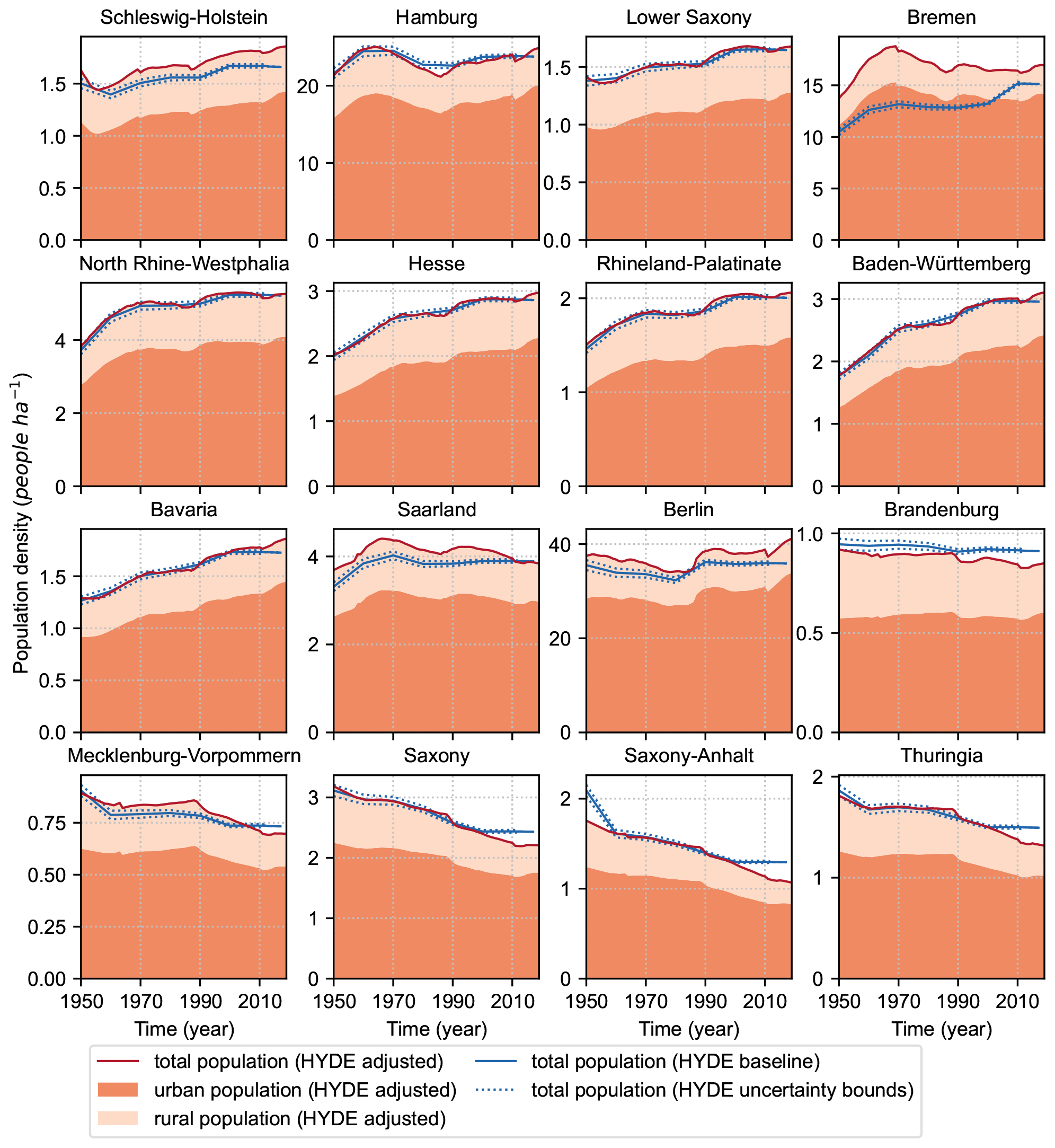
Figure 2 Population density estimated at NUTS-1 level from the original HYDE data for the period 1950–2017 (blue lines) and from the HYDE data that were adjusted to match statistical data for the period 1950–2019 (red lines). The original HYDE data include a baseline scenario and uncertainty bounds (lower and upper scenarios, dotted lines). The figure also shows the urban and rural population density for the adjusted HYDE data that were used to derive the N and P point source data in this study (shaded areas). Data source: HYDE data (Klein Goldewijk et al., 2017, 2022) are under a CC BY 4.0 licence. Statistical population data are from the Statistical Office of Germany (details in Table 2).

3.2 Protein supply

We use data of protein supply at the distribution level in Germany available from the Food and Agriculture Organization (FAO) for the year 1950 (FAO, 1951) and annually in the period 1961–2019 (FAO, 2021, 2022). We set the value in 1950 to the population-weighted average of the values provided for West and East Germany. Values for the years in the period 1951–1960 are filled using linear interpolation. The time series of the processed data at NUTS-0 (country) level is shown in Fig. 3a. Since no data are available at NUTS-1 level, we consider that the protein supply per capita is spatially uniform in Germany.

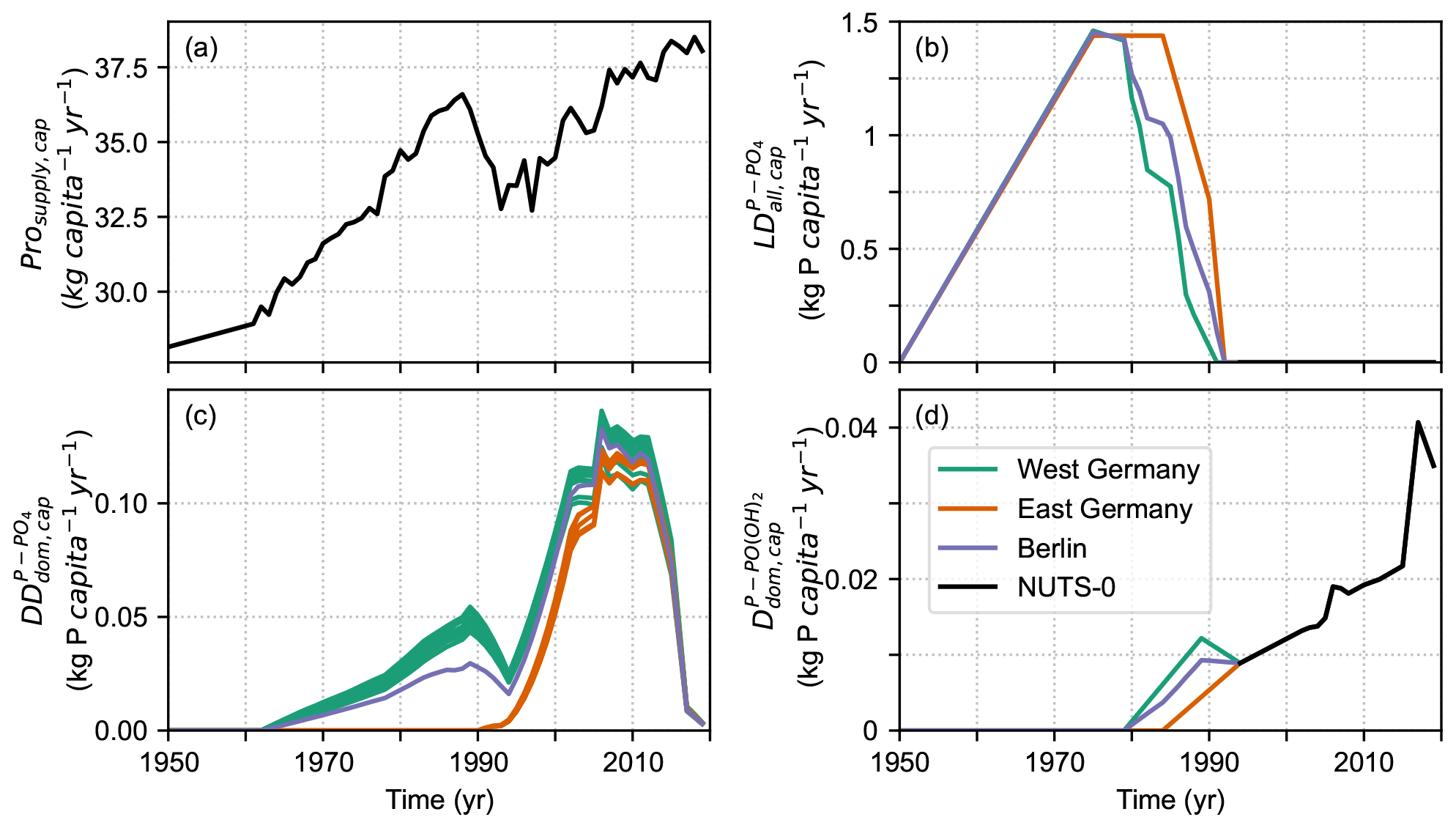
Figure 3 Processed protein and detergent data for the period 1950–2019: (a) protein supply per capita at NUTS-0 level (Pro_supply,cap); (b) total (domestic and industrial and commercial) laundry detergent phosphate P use per capita for West Germany, East Germany, and Berlin (LD${}_{\mathrm{all},\mathrm{cap}}^{\mathrm{P}-{\mathrm{PO}}_{\mathrm{4}}}$); (c) domestic dishwasher detergent phosphate P use per capita for each NUTS-1 region of West and East Germany and Berlin (DD${}_{\mathrm{dom},\mathrm{cap}}^{\mathrm{P}-{\mathrm{PO}}_{\mathrm{4}}}$); and (d) domestic detergent phosphonate P use per capita for West Germany, East Germany, and Berlin before 1992 and at NUTS-0 level from 1992 ($D_{\mathrm{dom},\mathrm{cap}}^{\mathrm{P}-\mathrm{PO}(\mathrm{OH}{)}_{\mathrm{2}}}$). For the period after 1991, domestic laundry detergent phosphate P use is equal to zero, while industrial and commercial laundry boosters contain phosphate, which we account for through the parameter LD${}_{\mathrm{ind},\mathrm{cap},\text{1991–2019}}^{\mathrm{P}-{\mathrm{PO}}_{\mathrm{4}}}$ that we vary within its uncertainty ranges (see Table 1). This is not reported in panel (b), which only shows the data before 1992. Data source: data in (a) come from © FAO with a CC BY-NC-SA 3.0 IGO licence. Data over the period 1961–2019 are provided in FAO (2021, 2022), and the 1950 value is estimated in this study as the average value over West and East Germany from FAO (1951). Data in (b) are the result of our own calculation from BMU (1989). Data in (c) and (d) are the result of our own calculations from data provided in © IKW (IKW, 2005, 2011, 2017, 2019) (https://www.ikw.org/impressum, last access: 21 September 2024) and dishwasher data from © Statistisches Bundesamt (SO-DE, 1979–2018). © Authors 2024. This figure is distributed under a CC BY-NC-SA 4.0 licence.

3.3 Detergent data

We reconstruct annual detergent P use per capita at NUTS-1 level for the period 1950–2019 based on national and sub-national data, as well as qualitative information. We include the main P compounds present in detergents, namely inorganic phosphates (BMU, 1989; Floyd et al., 2006; Glennie et al., 2002; Van Drecht et al., 2009) and phosphonates, which are poorly degradable organic compounds (Groß et al., 2012; Happel et al., 2021; IKW, 2019; Jaworska et al., 2002). We consider laundry detergents (LD) and automatic dishwasher detergents (DD), that are main sources of phosphate (Floyd et al., 2006; Glennie et al., 2002; Van Drecht et al., 2009) and phosphonate (Groß et al., 2012; Happel et al., 2021; IKW, 2019; Jaworska et al., 2002). Below, we describe the raw data and their processing to estimate total use of LD phosphate until around 1991 (Sect. 3.3.1), domestic DD phosphate use (Sect. 3.3.2), and domestic detergent phosphonate use (Sect. 3.3.3), defined in Eq. (2). To construct the LD phosphate and detergent phosphonate data, we collect statistical population data for West and East Berlin (see Table 2). To convert phosphate and phosphonate amounts to corresponding P equivalents, we adopt a P content of 0.326 for phosphate (PO${}_{\mathrm{4}}^{\mathrm{3}-}$) and of 0.382 for phosphonate (−PO(OH)₂) (Mehlhart et al., 2021).

3.3.1 Laundry detergent (LD) phosphate

We separately construct the temporal development of total (domestic and professional) LD phosphate use per capita in West and East Germany, where different regulations were in place before the reunification of Germany in 1990. For the state of Berlin, the phosphate LD use per capita is calculated as the population-weighted average of the values for West and East Germany that apply to the population of West and East Berlin, respectively.

In West Germany, the 1980 Phosphate Ordinance sets an upper limit to the phosphate content in LD for both the domestic and professional sectors (PHochstMengV, 1980). In addition, industries in West Germany self-committed to produce phosphate-free domestic LD in 1985 (IKW, 2019). For the period 1975–1988, we adopt the data provided by the German Federal Ministry of the Environment, Nature Conservation and Nuclear Safety (BMU, 1989). These data account for both the domestic and professional sector in West Germany only, and they are given for 9 years in the period 1975–1988. We then fill the missing years in the period 1975–1988 using linear interpolation.

In East Germany, to our knowledge, no regulations were put into place to limit the phosphate amount in LD before the Phosphate Ordinance (PHochstMengV, 1980) came into force in 1991 following German reunification (Kloepfer and Kröger, 1991). Since no data on detergent phosphate are available, we set the value of the consumption per capita to the average value for West Germany in the period 1975–1979. Further, we assume that this amount per capita remained unchanged until 1984. For the period 1985–1990, we consider that it followed similar temporal dynamics to that of other eastern European countries. From Table 3.2 in Glennie et al. (2002), we infer that between 1984 and 1990, LD phosphate consumption decreased by around 50 % for Hungary, Czech Republic, and Poland. Therefore, we set the 1990 value equal to 50 % of the 1984 value.

Since the early 1990s, domestic LD contain virtually no phosphate in Germany (IKW, 2011). “Normal” professional LD that is currently in use is also in general phosphate-free, but professional laundry boosters, utilised to wash heavily soiled textiles, can contain phosphate (Mehlhart et al., 2021). We consider that, in West Germany, household LD and “normal” professional LD were all phosphate-free from 1991 and that this occurred slightly after in East Germany (from 1992) because regulations were implemented later in the eastern region. We then perform linear interpolation to fill the gap between 1988 and 1991 for West Germany and between 1990 and 1992 for East Germany.

For the period 1950–1975, only qualitative information on LD phosphate can be found. Although the first LD containing phosphate was developed in the early 1930s (Foroutan-Rad, 1981, as cited in Nork, 1992; ZEODET, 2000), the use of phosphate as a detergent builder really started at the beginning of the 1950s (Berth et al., 1983, as cited in Nork, 1992). Therefore, we assume that the use of LD phosphate per capita was equal to 0 in 1950 in both West and East Germany, and we perform linear interpolation for the period 1950–1975. Figure 3b shows the processed data and Fig. S11 in the Supplement the raw data.

3.3.2 Domestic dishwasher detergent (DD) phosphate

We derive the domestic DD phosphate consumption per capita for the period 1950–2017. For this, we disaggregate domestic DD phosphate data at NUTS-0 level, provided by the German Cosmetic, Toiletry, Perfumery and Detergent Association, IKW (IKW, 2005, 2011, 2017, 2019), to NUTS-1 level using data of household dishwasher ownership at NUTS-1 level from the Statistical Office of Germany (SO-DE, 1979–2018). Below, we summarise the different processing steps and provide further details in Sect. S5.2.

Regarding the detergent data at NUTS-0 level, IKW provides data on the sale of domestic detergent phosphate for 14 years in the period 1989–2019. The 1989 value corresponds to West Germany only, while the later data (1994–2019) are available at NUTS-0 level. Since domestic LD has virtually no longer contained phosphate since the early 1990s in Germany (IKW, 2011), we consider that IKW household detergent phosphate data correspond exclusively to household DD phosphate over the period 1994–2019. We estimate the use per household at NUTS-0 level by dividing the IKW phosphate data by the number of households owning a dishwasher.

For the period prior to 1994, no DD phosphate data are available, since the data provided by IKW (for year 1989) include both LD and DD phosphate. We use qualitative information available on DD composition. A decline in DD phosphate occurred at the beginning of the 1990s due to the substitution of phosphate by metasilicates in DD (IKW, 2015). Owing to the corrosive nature of metasilicates, these were then removed from DD formulations from the mid-1990s onward and replaced back by phosphate; hence there was an increase in the phosphate content after the mid-1990s, as per IKW (IKW, 2015). After 2012, new formulations were introduced in household DD following the 2012 Detergent Regulation in the European Union, which limits the phosphate content in household DD (EC, 2012). This resulted in a sharp decrease in DD phosphate consumption. Given this qualitative information, we assume that, for the period 1950–1989, the formulation of DD phosphate was similar to the one in the years 2002–2012. Hence, we set the amount of DD phosphate per household during 1950–1989 to the average 2002–2012 value. We verify that our estimated total amount of DD phosphate used in 1989 for West Germany (around 9950 t yr⁻¹) is lower than the value provided by IKW (20 000 t yr⁻¹) for West Germany which includes all domestic detergent phosphate (LD and DD). We fill the values for the years in the period 1990–1993 as well as the years without the IKW inventory in the period 1994–2019 using linear interpolation.

To assess the total amount of DD phosphate use at NUTS-1 level, we multiply our estimated NUTS-0 amount per household by household dishwasher ownership data at NUTS-1 level. We derive the latter from household dishwasher ownership data from the Statistical Office of Germany for West Germany for the period 1962–2018, for East Germany for the period 1993–2018, and at NUTS-1 level in 2008. We infer that dishwashers were introduced in West Germany in 1963, since the data report a household dishwasher ownership of 0 % in 1962, and in East Germany in 1991 following German reunification, since the percentage of households that have a dishwasher is low in 1993 (2.7 %). We disaggregate the household dishwasher ownership data for West and East Germany to NUTS-1 level over the period 1950–2019. For this we use the 2008 NUTS-1 level data, and we assume that all NUTS-1 regions that belong to West and East Germany, respectively, followed the same temporal dynamics.

We then derive the domestic DD phosphate consumption per capita by dividing the NUTS-1 level domestic DD phosphate data by the corresponding NUTS-1 level population, assuming a spatially uniform DD phosphate detergent use per capita within a given NUTS-1 region. The degree of urbanisation has a limited impact on the percentage of households and population owning a dishwasher (see Supplement Sect. S5.2.3). We report the final processed data at NUTS-1 level in Fig. 3c.

3.3.3 Domestic detergent phosphonate

We estimate domestic detergent phosphonate use per capita for West and East Germany based on IKW data from 1989 for West Germany and from 1994 for East Germany (IKW, 2005, 2011, 2017, 2019) and based on qualitative information for the earlier period. We calculate the amounts for Berlin as the population-weighted average of the values for West and East Germany.

The domestic detergent phosphonate data from IKW are available for the year 1989 for West Germany and for the period 1994–2019 at NUTS-0 level. These quantities correspond to the total detergent phosphonate use in LD and DD (and possibly to a lesser extent other cleaning products). Domestic detergent phosphonate is an important component that showed large increases in the period 1994–2019. Notably, in 2019, it is equal to 7613 t yr⁻¹, which is almost 10 times the domestic DD phosphate amount (829 t yr⁻¹).

From the IKW data for the period 1994–2019, we assess the detergent phosphonate use per capita at NUTS-0 (country) level. We assume a spatially uniform value across Germany due to a lack of further spatial information. In addition, for West Germany, we assess the detergent phosphonate use per capita based on the 1989 IKW inventory, and we perform linear interpolation for the period between 1989 and 1994.

We utilise qualitative information on detergent phosphonate content for the period before 1989 for West Germany and before 1993 for East Germany. Phosphate-free LD typically contains phosphonate, while the phosphonate content in phosphate-based LD is between 0 to half that of phosphate-free LD (Table 2.2 in Glennie et al., 2002). In addition, domestic DD phosphonate was likely to be very small before 1980 in West Germany, since the proportion of households that had a dishwasher was limited (less than 15 % of households before 1978), and no DD had been used in East Germany before 1991. Consequently, we neglect the domestic phosphonate use before LD phosphate content started to be reduced in the 1980s; i.e. we set the phosphonate amount to 0 for the period 1950–1979 for West Germany and for the period 1950–1984 for East Germany. We then assume a linear increase in household detergent phosphonate use per capita for the period 1979–1989 for West Germany and 1984–1994 for East Germany. Figure 3d depicts the processed data and Fig. S14 in the Supplement the raw data.

3.4 Total population connection to the sewer system and to wastewater treatment

We collect and process data at NUTS-1 level of total population connection to the sewer system and to public WWTPs with different types of treatment, as well as to foreign and industrial WWTPs when available. These data come from various sources, mainly from statistical reports, and are complemented by qualitative information from Seeger (1999). In general, data are available from 1975 onward for West Germany and 1991 onward for East Germany. Table 2 provides an overview of these data. Figure 4 reports the final processed data and shows how the total population of the different NUTS-1 region was progressively connected to more advanced types of wastewater treatment. The data are briefly described below, while Sect. S6 in the Supplement reports further details, including an analysis on the value of our data compared to the readily available data provided by the statistical office of the European Union (Eurostat, 2016, 2023).

For the state of Berlin, we consider that all wastewater that is collected in the sewer system but not treated in WWTPs is applied to agricultural soils in sewage farms (Fig. 4), given the importance of this type of treatment, as documented, for instance, in Lottermoser (2012). This occurs up to the year 1982, as in later years the data indicate that all wastewater collected in the sewer system is treated in WWTPs. We do not consider sewage farms in other NUTS-1 regions due to a lack of information.

Not only do we account for wastewater treated in public WWTPs via collection in the sewer system but also, when the data are available, for wastewater collected in cesspits (sealed tanks) and transported by trucks to public WWTPs. We do not consider independent treatment in small wastewater treatment plants because of a lack of data on such treatment. We consider that the resident population of a given NUTS-1 region is connected to WWTPs located in that NUTS-1 region only. An exception is the state of Berlin for which a large part of the population is connected to WWTPs in the neighbouring state of Brandenburg (35 %–65 % of the population over the period 1991–2019). We consider that the part of the population of Berlin whose wastewater is handled in Brandenburg is all connected to WWTPs, while the part of the population of Berlin whose wastewater is handled in Berlin can be either connected to sewage farms or WWTPs or not connected to the public wastewater system.

Regarding the data of population connection to the different types of wastewater treatment, most data refer to the population treated in WWTPs located in a given NUTS-1 region, and we consider that the same relative proportions of the different treatment types apply to the resident population (apart from Berlin and Brandenburg, as explained above). In a few cases, we use data of the volume of wastewater treated following the different treatment types to derive temporal changes for the population connection to these treatment types.

For the earlier years where statistical data are not provided, we use qualitative information provided by Seeger (1999) to set a starting year of the different treatment types. Accordingly, we assume that sewer connection started in 1880, primary wastewater treatment in 1910, secondary treatment in 1950, and tertiary treatment with targeted N and P removal in 1980 in West Germany and 1990 in East Germany. We then consider a linear development up to the first year with available data. This is consistent with the study of Seeger (1999), in which the development of wastewater treatment in Germany is described as a “steady process”. Regarding the population connected to WWTPs via cesspits, in the absence of further information, we consider that it is equal to zero before the first year with data and after the last year with data. We perform linear interpolation between the years for which population connection data are not provided.

Figure 4 Processed fractions of total population connection at NUTS-1 level for the period 1950–2019 that were used to derive the N and P point source data in this study. Specifically, the figure reports the fraction of the total population that is not connected to the sewer system nor to WWTPs (NoCon_all), the fraction of total population connected to the sewer system but not to WWTPs (T0_all), the fraction of total population connected to sewage farms (TFarm_all), the fraction of total population connected to primary (mechanical) treatment (T1_all), the fraction of total population connected to secondary (biological) treatment and tertiary (advanced) treatment without targeted N removal ($T{\mathrm{23}}_{\mathrm{all}}^{\mathrm{noN}}$), and the fraction of total population connected to tertiary treatment with target N removal ($T{\mathrm{3}}_{\mathrm{all}}^{\mathrm{N}}$). Figure S18 in the Supplement further reports on development of $T{\mathrm{23}}_{\mathrm{all}}^{\mathrm{noP}}$ and $T{\mathrm{3}}_{\mathrm{all}}^{\mathrm{P}}$, which take similar values to $T{\mathrm{23}}_{\mathrm{all}}^{\mathrm{noN}}$ and $T{\mathrm{3}}_{\mathrm{all}}^{\mathrm{N}}$. Data source: the data shown in this figure were elaborated in this study building on data from the statistical offices of Germany and the different federal states as well as additional sources, as detailed in the Supplement, Sect. S6.

EEA, 2023b(Büttner, 2020)

Table 3 Description of the observational data of WWTPs incoming and outgoing N and P loads used for downscaling and model evaluation.

PE is the population equivalent. ^a The spatial extent is Germany for all data. ^b The DE dataset mostly includes WWTPs that have a design capacity lower than 2000 PE, but it also encompasses some WWTPs that have a design capacity higher than or equal to 2000 PE. ^c For each WWTP, data are available either for year 2015 or for year 2016. ^d The nutrient species, WWTP types, and load types vary across NUTS-1 regions and data sources (see details in the Supplement, Sect. S8, in particular Tables S45 and S60). ^e Period over which some data are available. The temporal extent varies across NUTS-1 regions, nutrient species, WWTP types, load types (see details in the Supplement Sect. S8, in particular Tables S45 and S60). ^f © European Environment Agency (EEA), CC BY 4.0 licence. ^g Data collection was supported by research projects of UFZ under a confidentiality agreement with the German states' authorities.

3.5 Observations of WWTP incoming and outgoing N and P emissions

We construct datasets of observations of WWTP N and P emissions though the collection and processing of data from different sources, as summarised in Table 3. We derive a gridded map of WWTP load from data at WWTP level (presented in Sect. 3.5.1) to downscale our NUTS-1 level N and P point source estimates (as explained in Sect. 2.2). Data at NUTS-1 level (presented in Sect. 3.5.2) are used to estimate the parameters/coefficients of the N and P point sources model and to evaluate our N and P point source estimates (as explained in Sect. 4).

3.5.1 Observations of WWTP incoming and outgoing N and P emissions at WWTP level

We merge two datasets of observations of WWTP incoming and outgoing N and P loads around the year 2016, namely (1) the Urban Waste Water Treatment Directive (UWWTD) Waterbase dataset of the European Environmental Agency (EEA, 2023b, hereafter referred to as the EU dataset), including 4302 WWTPs in 2016, and (2) data coming from the authorities of the German federal states and made available in the dataset of Büttner (2020) (hereafter referred to as the DE dataset), including 6361 WWTPs for the year 2015 or 2016 depending on the plants. We could not derive WWTP loads beyond the years 2016, since the EU dataset only (and not the DE dataset) provides data beyond 2016 (namely every 2 years in the period 2010–2018). The EU dataset consists of WWTPs that treat wastewater in agglomerations larger than the 2000 population equivalent (PE). This is why this dataset needs to be complemented by the DE dataset, which includes WWTPs for agglomerations smaller than 2000 PE. We refer to Supplement Sect. S9 for details on the data processing, while a summary is reported below.

The combined dataset encompasses 9006 WWTPs, since we establish that 1657 WWTPs are present in both the EU and DE datasets. To avoid duplication, we merged the records for these WWTPs by selecting the coordinates from the DE dataset. We do not account for the uncertainty in the coordinates arising from the discrepancies between the EU and DE dataset, since the distance calculated between the coordinates reported in the two datasets is mostly within our target grid resolution of 0.015625°. We fill the missing values of the N and P load using values for the other years provided in the EU dataset when available, or we perform extrapolation based on values of the WWTP entering load expressed in PE provided in both the EU and DE datasets. We find that these filled values account for less than 8 % of the total load at NUTS-1 level. We also verify that the uncertainty in the loads of the combined dataset is generally contained. The uncertainty results from the low precision of the load values reported in the EU dataset and the discrepancies in the values of the load between the EU and DE dataset for the 1657 overlapping WWTPs and our gap-filling procedure. Our processed dataset comprises values of the incoming and outgoing N and P loads for over 99 % of the 9006 WWTPs, while only for 39 WWTPs are no values at all of the N and P loads able to be estimated, and for 16 WWTPs no value of the incoming N and P loads and the outgoing N loads can be derived.

Finally, we create a gridded map of WWTPs' outgoing N and P emissions at a resolution of 0.015625°. For this, for each grid cell, we sum the mean values of the load (average of the lower and upper bound estimated) over all WWTPs that fall within that grid cell. We move the location of 137 WWTPs between 500 and 2500 m to ensure that they fall within the NUTS-1 regions reported in the EU and DE datasets.

3.5.2 Observations of WWTP incoming and outgoing N and P emissions at NUTS-1 level

We compile observational data of public WWTP incoming and outgoing N and P load at NUTS-1 level from different reports of the statistical offices of Germany and the federal states, as well as situation reports of the authorities of the German federal states (see details in the Supplement, Sect. S8 and Figs. S28–S31). The data span the period 1987–2020, depending on the NUTS-1 regions. While P data always correspond to total P, N load data are provided either as inorganic N or as total N. Some data only include WWTPs with a design capacity higher than 2000 PE, and we do not further process these data. Section S8 in the Supplement provides details on the processing, which is summarised in the following paragraph.

We find total N observations for half of the NUTS-1 regions, while inorganic N and total P observations are available for all NUTS-1 regions. Since our point source estimation focuses on total N, for the NUTS-1 regions for which total N data are not provided at all or for a limited time period, we estimate total N from inorganic N observations for outgoing N load. For this, we apply a ratio of total N to inorganic N that we derive based on the relative value of these two quantities during their common periods of availability for the different NUTS-1 regions. We derive lower- and upper-bound estimates of the outgoing load when possible, accounting for the uncertainties in the total N to inorganic N ratio and for the fact that load measurements may not include all WWTPs (even for data referring to WWTPs of all design capacities).

We note that incoming N and P load data, which are mostly provided in the situation reports, may result from both measurements and estimates based on the PE and a constant coefficient of the N and P emissions per PE when observations are missing (LU-RP and MKUEM-RP, 2021; MUNLV-NW, 2020). However, this uncertainty cannot be quantified, since no information on the relative proportion of the measured and estimated loads in the NUTS-1 level data is provided. In addition, data of incoming N loads cannot be obtained for all NUTS-1 regions.

4 Methods for parameter estimation and model evaluation at NUTS-1 level

To estimate the 18 model parameters (coefficients), we generate a prior parameter sample of size 100 000 using Latin hypercube sampling and uniform distributions, from the ranges reported in Table 1, and using the SAFE toolbox (Pianosi et al., 2015). These ranges were either determined from previous studies, in particular Morée et al. (2013), or from our collection and processing of additional data (details in the Supplement, Sect. S3). Food waste data provided by FAO and SIK (2011) and Noleppa and Cartsburg (2015) are used to establish the range for the fraction of protein supply wasted at the distribution and consumption level ($f_{\mathrm{waste}}^{\mathrm{pro}}$). Data of industrial and commercial laundry and dishwasher detergent phosphate use in 2015 and industrial and commercial detergent phosphonate use in 2008 and 2015 from the German Industry Association for Hygiene and Surface Protection for Industrial and Institutional Applications (IHO) are adopted to set the range for detergent parameters ($f_{\mathrm{ind}:\mathrm{dom},\text{1950–2012}}^{\mathrm{DD},\mathrm{P}-{\mathrm{PO}}_{\mathrm{4}}}$, $f_{\mathrm{ind}:\mathrm{dom},\text{1950–2015}}^{\mathrm{D},\mathrm{P}-\mathrm{PO}(\mathrm{OH}{)}_{\mathrm{2}}}$, and LD${}_{\mathrm{ind},\mathrm{cap},\text{1991–2019}}^{\mathrm{P}-{\mathrm{PO}}_{\mathrm{4}}}$).

For each of the 16 NUTS-1 regions of Germany, we perform Monte Carlo simulations for the period 1950–2019 using the prior parameter sample, and we identify an ensemble of posterior (behavioural) simulations that are most consistent with both the N and P outgoing load observations described in Sect. 3.5.2. We thereby account for the uncertainty arising in particular from the observations that are uncertain and have a limited temporal coverage. Specifically, we select the 100 (behavioural) simulations that have the lowest value of the sum of the two root mean square errors between the observed and simulated WWTP outgoing load for N and P. The root mean square error for the ith NUTS-1 region and jth posterior simulation (realisation) is computed as follows:

$$\begin{array}{}\text{(21)}& \mathrm{RMSE}(i,j)=\sqrt{{\displaystyle \frac{{\sum }_{t\in E_{\mathrm{obs}\left(i\right)}}\mathrm{err}(t,i,j{)}^{\mathrm{2}}}{N_{\mathrm{obs}}\left(i\right)}}}{\displaystyle \frac{\mathrm{100}}{{\mathit{\mu }}_{\mathrm{obs}}\left(i\right)}},\end{array}$$

where RMSE(i,j) (%) is the root mean square error, err$(t,i,j)$ (kg yr⁻¹) is the error between the simulated and observed (N or P) load at year t, E_obs(i) is the ensemble of years for which observations are available, N_obs(i) is the number of observations, and μ_obs(i) (kg yr⁻¹) is the mean of the observations. RMSE is normalised by the mean of the observations to allow comparability of the realisation performance across nutrient species (N and P) and NUTS-1 regions. Since the observations can have a lower and upper uncertainty bound (as explained in Sect. 3.5.2), we calculate the error between simulations and observations as follows:

$$\begin{array}{}\text{(22)}& \begin{array}{rl}\mathrm{err}(t,i,j)& =max\left(X_{\mathrm{obs}}^{\mathrm{lb}}\right(t,i)-X_{\mathrm{sim}}(t,i,j),\mathrm{0})\\ & +max\left(X_{\mathrm{sim}}\right(t,i,j)-X_{\mathrm{obs}}^{\mathrm{ub}}(t,i),\mathrm{0}),\end{array}\end{array}$$

where $X_{\mathrm{sim}}(t,i,j)$ (kg yr⁻¹) is the simulated load, and $X_{\mathrm{obs}}^{\mathrm{lb}}(t,i)$ (kg yr⁻¹) and $X_{\mathrm{obs}}^{\mathrm{ub}}(t,i)$ (kg yr⁻¹) are the lower and upper bounds of the observations, respectively. From Eq. (22), the error is equal to zero when the simulation is within the observation uncertainty bounds.

We also calculate two additional metrics to evaluate the accuracy of the selected 100 posterior simulations with respect to the observations, namely the mean absolute error for the ith NUTS-1 region and jth posterior realisation, denoted as MAE(i,j) (%), and the distance of the observations to the posterior ensemble for the ith NUTS-1 region and at time t, denoted as DIST(t,i) (%), defined as follows:

$$\begin{array}{}\text{(23)}& {\displaystyle }\mathrm{MAE}(i,j)={\displaystyle \frac{{\sum }_{t\in E_{\mathrm{obs}\left(i\right)}}\mathrm{err}(t,i,j)}{N_{\mathrm{obs}}\left(i\right)}}{\displaystyle \frac{\mathrm{100}}{{\mathit{\mu }}_{\mathrm{obs}}\left(i\right)}}\text{(24)}& {\displaystyle }\mathrm{DIST}(t,i)=\mathrm{100}{\displaystyle \frac{\begin{array}{c}max\left(X_{\mathrm{obs}}^{\mathrm{lb}}\right(t,i)-X_{\mathrm{sim}}^{\mathrm{ub}}(t,i),\mathrm{0})\\ +max\left(X_{\mathrm{sim}}^{\mathrm{lb}}\right(t,i)-X_{\mathrm{obs}}^{\mathrm{ub}}(t,i),\mathrm{0})\end{array}}{\left(\frac{X_{\mathrm{obs}}^{\mathrm{lb}}(t,i)+X_{\mathrm{obs}}^{\mathrm{ub}}(t,i)}{\mathrm{2}}\right)}},\end{array}$$

where $X_{\mathrm{sim}}^{\mathrm{lb}}(t,i)$ (kg yr⁻¹) and $X_{\mathrm{sim}}^{\mathrm{ub}}(t,i)$ (kg yr⁻¹) are the lower bound (minimum value over the 100 realisations) and upper bound (maximum value over the 100 realisations) of the posterior simulation ensemble, respectively. DIST is equal to zero when the observation uncertainty interval intersects the simulation uncertainty interval, which corresponds to a high accuracy of the posterior ensemble.

We further evaluate the consistency of the posterior realisations by comparing them visually with the additional observations of WWTP outgoing load available, that is observations of N inorganic load as well as N and P load for WWTPs that have a design capacity larger than 2000 PE (see Sect. 3.5.2). We also assess the performance metrics of Eqs. (21), (23), and (24) for the WWTP incoming total N and P load described in Sect. 3.5.2, as an another plausibility check to our reconstructed dataset. Due to the limited coverage and uncertainty in data of WWTP incoming total N and P load, we only use these data for evaluation purposes and not for the identification of the posterior realisations.

In our realisations, the N and P emissions for Berlin come from the wastewater that is both generated and handled in Berlin. For Brandenburg, N and P emissions include the part of wastewater that is generated in Berlin (which corresponds to a large part of the population of Berlin, as detailed in Sect. 3.4) along with its own (Brandenburg) contribution.

5 Results

5.1 Evaluation of the point source estimates at NUTS-0 and NUTS-1 level

The behavioural realisations show a good consistency with the observations of WWTP outgoing N and P loads ($J_{\mathrm{ps},\mathrm{wwtpOut},\mathrm{all}}^{\mathrm{N}}$ and $J_{\mathrm{ps},\mathrm{wwtpOut},\mathrm{all}}^{\mathrm{P}}$, respectively) for the 16 NUTS-1 regions. Minimum values of RMSE and MAE across the 100 behavioural realisations, obtained for the best-performing behavioural realisations, are lower than 17.5 % and 15.1 %, respectively, and maximum values are lower than 24 % and 20 %, respectively (Table 4). We also find that the posterior realisation ensemble of the WWTP outgoing N load, which is bounded by their respective minimum and maximum values across the 100 posterior realisations, intersects all observation uncertainty bounds for the regions of Saarland, Brandenburg, and Mecklenburg-Western Pomerania (values of DIST are equal to 0 in Table 4). In all other regions, the posterior realisations of the WWTP outgoing N and P load captures only some of the observational bounds, with positive values of DIST. Nonetheless, the mean value of DIST across the observations is always lower than 12 %, which demonstrates an overall good accuracy of the WWTP outgoing load realisations. From Figs. 5 and 6, we qualitatively appreciate the consistency of the posterior realisation ensembles with the observational data that were used for parameter estimation (dark-brown circles and crosses) and additional data, in particular the observations for WWTPs with a design capacity higher than 2000 PE for Saxony-Anhalt and Thuringia (yellow and light-green dots in Figs. 5o and p and 6o and p). The outgoing P load for the NUTS-1 region of Schleswig-Holstein shows relatively lower performance, with values of RMSE and MAE in the range 83 %–95 % and 30 %–60 %, respectively (Table 4). From Fig. 6a, we see that the posterior realisation ensemble includes all observations except one in 1987, which is underestimated. Further observations around this time period would be required to determine whether this mismatch is due to errors in the observations or missing P contributions in our model and input data.

We quantitatively evaluate the plausibility of the posterior realisations of WWTPs' incoming N and P load ($J_{\mathrm{wwtpIn},\mathrm{all}}^{\mathrm{N}}$ and $J_{\mathrm{wwtpIn},\mathrm{all}}^{\mathrm{P}}$, respectively) when observations are available (Table 4, Figs. S36 and S37 in the Supplement). For incoming N load, performances are overall satisfying, with average values of RMSE and MAE in the range 7.5 %–20.2 % and 6.2 %–16.3 %, respectively, although the performance varies across the posterior ensembles, with values of up to 30 %–40 % for Bremen; Rhineland-Palatinate; and Mecklenburg-Western Pomerania, where, however, only one observation point is available. DIST also demonstrates good skill in modelled estimates, with values lower than 20 % for all NUTS-1 regions and always equal to zero for five out of the eight NUTS-1 regions with observations. Additional observations for WWTPs with a design capacity higher than 2000 PE confirm the plausibility of the realisations for Lower Saxony and Saxony-Anhalt but suggest that our realisation underestimates the load in Saarland between 2008 and 2019 (Fig. S36). For incoming P load, the posterior realisations tend to underestimate the observations. The performance is in general lower than for the incoming N load and the outgoing N and P load, with average values of RMSE and MAE both in the range of 12.7 %–40.1 % and average values of DIST in the range 0 %–26 %.

Figures 5 and 6 depict a substantial uncertainty reduction in the posterior realisation ensemble (dark-grey-shaded areas) compared to the prior realisation ensemble (light-grey-shaded areas) of the WWTP outgoing N and P load, in particular over the most recent period. Specifically, the width of the posterior realisation ensemble (delimited by the minimum and maximum values across the posterior realisations) normalised by the mean estimate is, for most NUTS-1 regions, 1.17 to 7.7 time larger on average over the (past) period without observations compared to the (recent) period with observations. The latter starts between 1987 and 2008, depending on the NUTS-1 regions and whether it is N or P. Two NUTS-1 regions show a different pattern, namely Schleswig-Holstein, where the normalised width is larger over the period with observations, and North Rhine-Westphalia, where the normalised width is similar over the two time periods. Nevertheless, the absolute width of the posterior realisation ensemble (expressed in kg ha⁻¹ yr⁻¹) is always larger (1.8 to 63.5 times on average) over the period without observations. Specifically, the average width of the posterior ensemble for the WWTP outgoing N (P) load is in the range 0.9–29 kg ha⁻¹ yr⁻¹ (0.11–4.3 kg ha⁻¹ yr⁻¹) over the period without observations and in the range 0.03–2.2 kg ha⁻¹ yr⁻¹ (0.00–0.15 kg ha⁻¹ yr⁻¹) over the period with observations. Further details of the region-wise uncertainty intervals are reported in the Supplement, Tables S80 and S81, for both the WWTP outgoing load and the total point sources. For the other model variables beyond the total and treated point sources, the uncertainty reduction in the posterior compared to the prior ensemble is in general not as pronounced, as can be seen from Supplement Figs. S36, S37 for WWTP incoming N and P load and from Figs. S51–S61 for other pathways. This is likely related to the fact that no observational data of these components are used to constrain their respective parameters.

Table 4 Performance metrics calculated between the 100 posterior realisations of the WWTP incoming and outgoing N and P load and the observations for the 16 NUTS-1 regions of Germany. NA – not available

Note that RMSE is the root mean square error (Eq. 21), MAE is the mean absolute error (Eq. 23), DIST is the distance of the observations to the posterior realisation ensemble (Eq. 24), $J_{\mathrm{ps},\mathrm{wwtpOut},\mathrm{all}}^{\mathrm{N}}$ is the WWTP outgoing N load, $J_{\mathrm{ps},\mathrm{wwtpOut},\mathrm{all}}^{\mathrm{P}}$ is the WWTP outgoing P load, $J_{\mathrm{wwtpIn},\mathrm{all}}^{\mathrm{N}}$ is the WWTP incoming N load, and $J_{\mathrm{wwtpIn},\mathrm{all}}^{\mathrm{P}}$ is the WWTP incoming P load. The numbers indicate the mean, minimum (min), and maximum (max) values: mean${}_{\min }^{\max }$. For RMSE and MAE, the mean, maximum, and minimum values are calculated over the posterior simulations, while for DIST they are calculated over time.

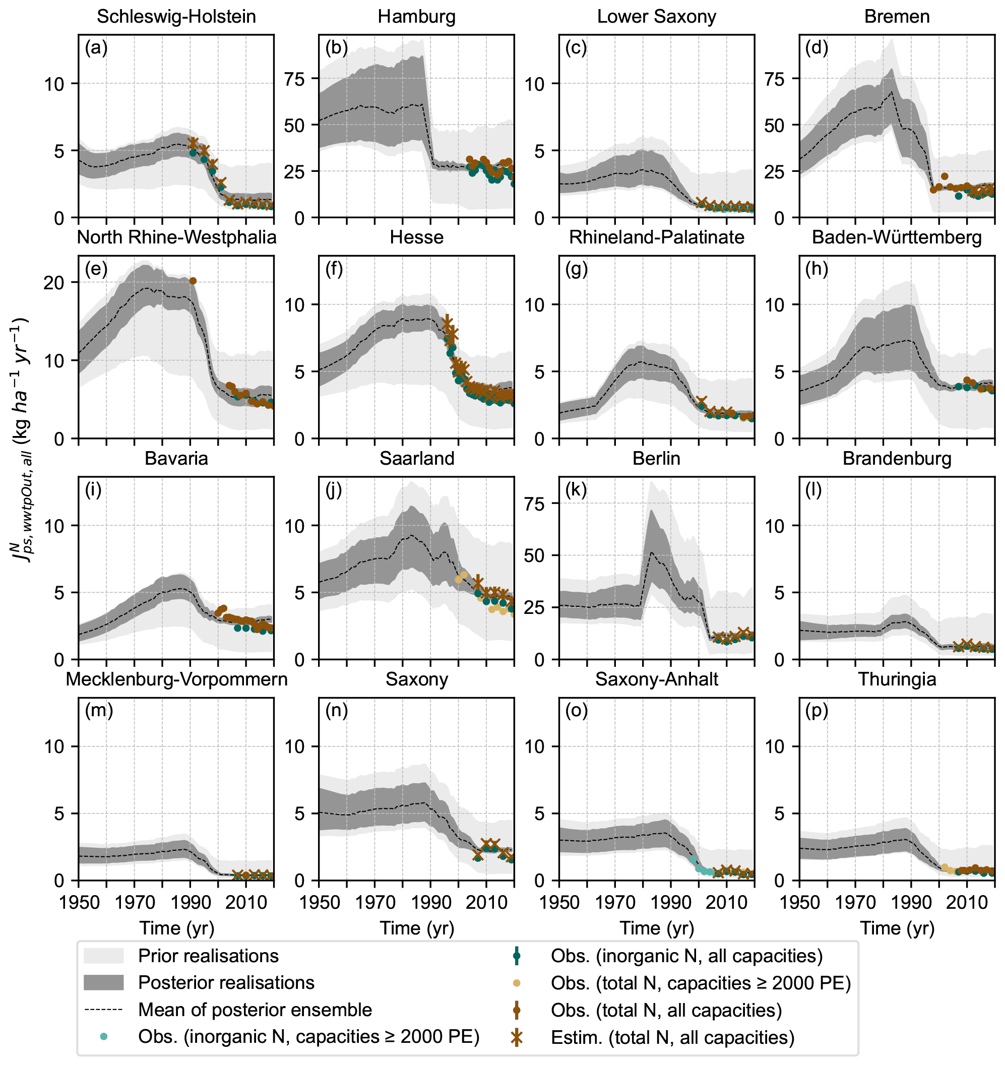
Figure 5 WWTP outgoing N loads $J_{\mathrm{ps},\mathrm{wwtpOut},\mathrm{all}}^{\mathrm{N}}$ (kg ha⁻¹ yr⁻¹) from the prior and posterior model realisations (grey-shaded areas and dashed lines), observations (coloured circles), and our estimates of total N load from inorganic N load data (dark-brown crosses) at NUTS-1 level for the period 1950–2019. The shaded areas delineate the minimum and maximum values of the 100 000 prior realisations (light grey) and the 100 posterior realisations (dark grey). Observational values are shown for both the ensemble of WWTPs with a design capacity higher than 2000 PE (light green and brown) and for all WWTPs (dark green and brown). Some observations are reported with error bars that depict the upper and lower bound estimates, while the markers (circles or crosses) represent the average value. The scale on the y axis is the same for all NUTS-1 regions but the city states (Hamburg, Bremen, and Berlin) and North Rhine-Westphalia, for which the loads are much higher compared to the other NUTS-1 regions. Data source: observational data come from the statistical offices of Germany and the federal states and from the authorities of the federal states. The uncertainty intervals on the observations were processed in this study. The estimates of total N represented with brown crosses were derived in this study from inorganic N data. Details on NUTS-1 observational data sources and processing are in the Supplement, Sect. S8. © Authors 2024. This figure is distributed under a CC BY-NC-SA 4.0 licence.

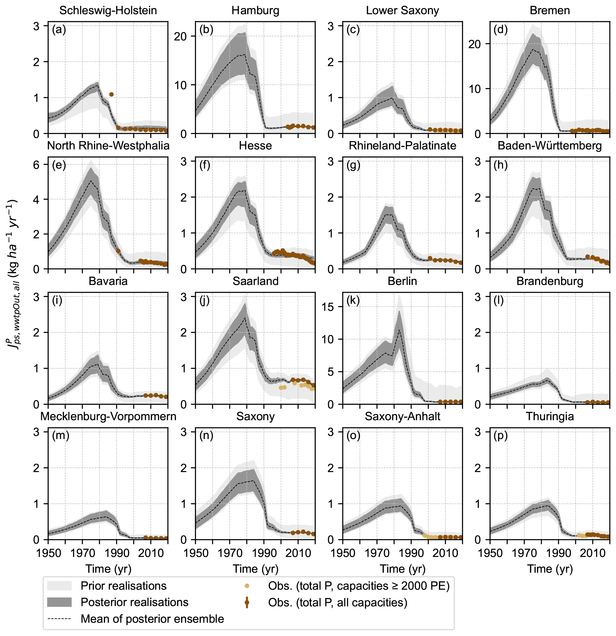
Figure 6 WWTP outgoing P loads $J_{\mathrm{ps},\mathrm{wwtpOut},\mathrm{all}}^{\mathrm{P}}$ (kg ha⁻¹ yr⁻¹) from the prior and posterior model realisations (grey-shaded areas and dashed lines) and observations (coloured circles) at NUTS-1 level for the period 1950–2019. The shaded areas delineate the minimum and maximum values of the 100 000 prior realisations (light grey) and the 100 posterior realisations (dark grey). Observational values are shown both for the ensemble of WWTPs with a design capacity higher than 2000 PE (light brown) and for all WWTPs (dark brown). Some dark-brown circles are reported with error bars that depict the upper and lower bound estimates, while the circles represent the average value. The scale on the y axis is the same for all NUTS-1 regions but the city states (Hamburg, Bremen, and Berlin) and North Rhine-Westphalia, for which the loads are much higher compared to the other NUTS-1 regions. Data source: observational data come from the statistical offices of Germany and the federal states and from the authorities of the federal states. The uncertainty intervals on the observations were processed in this study. Details on NUTS-1 observational data sources and processing are in the Supplement, Sect. S8. © Authors 2024. This figure is distributed under a CC BY-NC-SA 4.0 licence.

These differences in uncertainty bounds between the periods with and without observations can be interpreted in terms of parameter sensitivity. Table 5 shows that the parameter estimation procedure allows the ranges of a few parameters to be reduced appreciably, namely (1) the efficiencies of tertiary treatment with targeted N and P removal (eff${}_{{\mathrm{3}}^{\mathrm{N}}}^{\mathrm{N}}$ and eff${}_{{\mathrm{3}}^{\mathrm{P}}}^{\mathrm{P}}$) and (2) the efficiencies of secondary and tertiary treatment without targeted N and P removal (eff${}_{{\mathrm{23}}^{\mathrm{noN}}}^{\mathrm{N}}$ and eff${}_{{\mathrm{23}}^{\mathrm{noP}}}^{\mathrm{P}}$) to a lesser extent and for some NUTS-1 regions only. This also reflects the fact that these two types of wastewater treatment tend to be more prevalent during the (recent) period with observations (Fig. 4). We observe that the posterior parameter ranges for eff${}_{{\mathrm{3}}^{\mathrm{N}}}^{\mathrm{N}}$ and eff${}_{{\mathrm{3}}^{\mathrm{P}}}^{\mathrm{P}}$ vary across NUTS-1 regions. Regarding eff${}_{{\mathrm{23}}^{\mathrm{noN}}}^{\mathrm{N}}$ and eff${}_{{\mathrm{23}}^{\mathrm{noP}}}^{\mathrm{P}}$, the higher values tend to be discarded in the posterior sample for some NUTS-1 regions. Notably, additional parameters have an impact on the simulated N and P outgoing load during the period with observations for at least some of the NUTS-1 regions. This mostly regards parameters that control the magnitude of the human N and P gross emissions (namely $f_{\mathrm{waste}}^{\mathrm{pro}}$, $f_{\mathrm{pro}}^{\mathrm{N}}$, and $f_{\mathrm{intake}}^{\mathrm{N}:\mathrm{P}}$), the fractions of industrial and commercial to domestic N and P gross emissions in 2000 (namely $f_{\mathrm{ind}:\mathrm{dom},\mathrm{2000}}^{\mathrm{N}}$ and $f_{\mathrm{ind}:\mathrm{dom},\mathrm{2000}}^{\mathrm{P}}$), and the fraction of N and P emissions lost during wastewater collection and transport ($f_{\mathrm{loss},\mathrm{transport}}^{\mathrm{N},\mathrm{P}}$). Although the ranges of these parameters cannot be reduced in the posterior parameter sample because of parameter interactions, their distributions are constrained (the posterior distributions deviate from the prior distributions in the Supplement, Fig. S35). During the period without observations, parameters that could hardly be constrained may have a significant impact on the simulations. This for example can be the fractions of industrial and commercial to domestic N and P gross emissions in 1950 (namely $f_{\mathrm{ind}:\mathrm{dom},\mathrm{1950}}^{\mathrm{N}}$ and $f_{\mathrm{ind}:\mathrm{dom},\mathrm{1950}}^{\mathrm{P}}$) and the N and P removal efficiencies for primary treatment (eff${}_{\mathrm{1}}^{\mathrm{N}}$ and eff${}_{\mathrm{1}}^{\mathrm{P}}$). Primary treatment was indeed widespread before 1990 (Fig. 4).

At NUTS-0 (country) level, we assess the consistency of the WWTP outgoing N and P load from the mean behavioural realisation (dark-orange-shaded areas in Fig. 7a, b) with the corresponding data provided by the Germany Environmental Agency for the period 1987–2016 (UBA, 2020) (dotted red line in Fig. 7a, b). The UBA data (Behrendt et al., 2000; Fuchs et al., 2010, 2017, 2022) were constructed from WWTP data for the recent period, while they are based on further modelling assumptions for the earlier period to compensate for the paucity of data. Hence, similar to our data, we expect that the UBA data have larger uncertainties for earlier years compared to the recent ones. The relative differences between our estimates and the UBA data with respect to the UBA data vary over time between −23.6 % and 6.8 % for the N load and between −45.5 % to 2.5 % for the P load, a negative value indicating that our realisations are lower then the UBA value and vice versa. A relatively good match is found for the recent period. Specifically, the error is always within ±10 % from 2002 onward for the N load and from 2006 onward for the P load. The largest relative difference is found for the year 1987 for N (−23.6 %; −2 kg ha⁻¹ yr⁻¹) and for the year 1994 for P (−45.5 %; −0.32 kg ha⁻¹ yr⁻¹). These results confirm the higher uncertainty in WWTP outgoing load estimates before the 2000s compared to the 2000s and 2010s when more data are available to constrain the calculations. Similar observations can be made when considering all 100 posterior realisations beyond the mean value (Supplement Figs. S38, S39).

Table 5 Lower and upper values of the parameters in the prior sample and in the posterior sample for each NUTS-1 region and percentage reduction in the parameter ranges (Δ) in the posterior compared to the prior distribution (we report only the four parameters for which Δ is higher than 20 % for at least one NUTS-1 region).

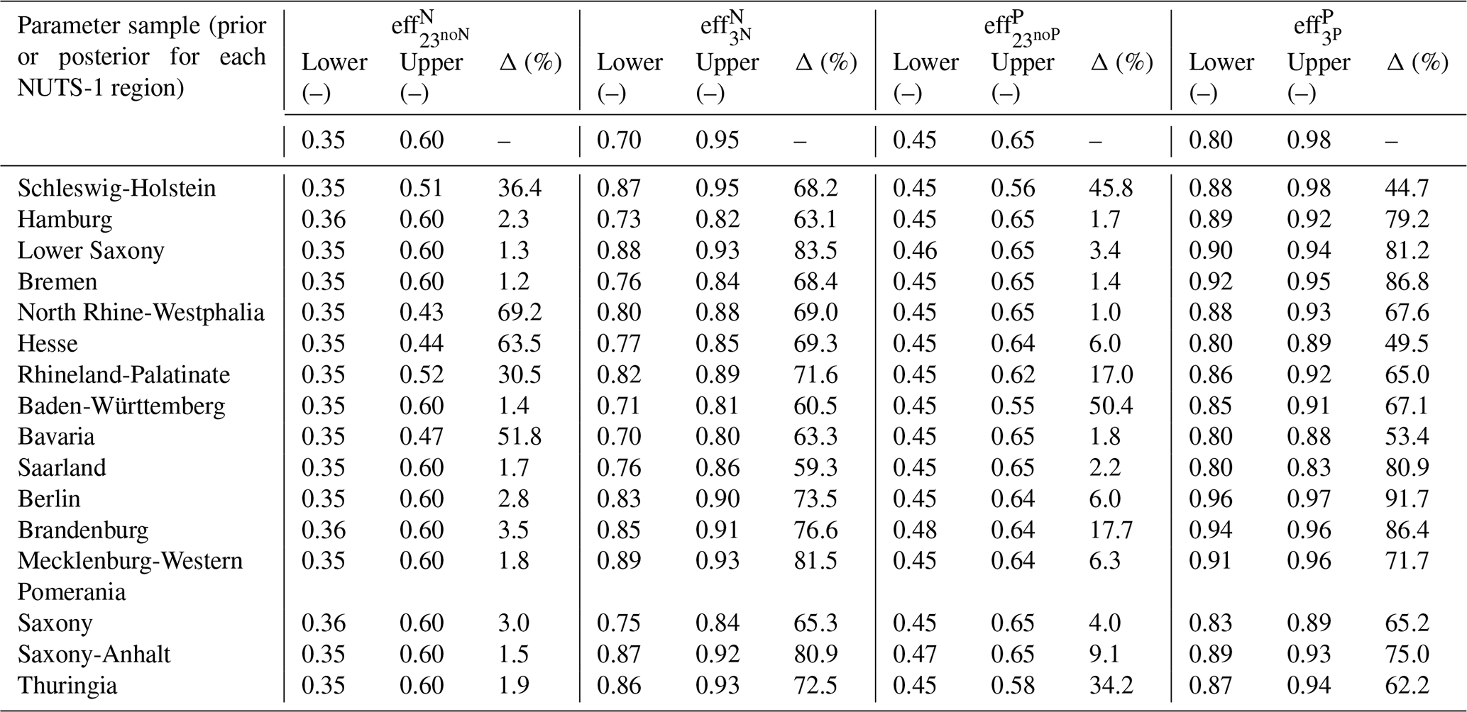
The parameters are defined in Table 1. The prior parameter sample is the same for each NUTS-1 region. For a given parameter, the percentage reduction in the range (Δ (%)) is calculated as $\mathrm{\Delta }=\mathrm{100}(\mathrm{1}-\frac{{\mathrm{Upper}}_{\mathrm{posterior}}-{\mathrm{Lower}}_{\mathrm{posterior}}}{{\mathrm{Upper}}_{\mathrm{prior}}-{\mathrm{Lower}}_{\mathrm{prior}}})$, where Upper_posterior and Lower_posterior are the upper and lower values, respectively, in the posterior parameter sample, and Upper_priori and Lower_prior are the upper and lower values, respectively, in the prior parameter sample.

5.2 Fate of N and P gross emissions at NUTS-0 and NUTS-1 level (1950–2019)

Figure 7 presents the fate of the N and P gross emissions at NUTS-0 level from the mean of the posterior realisations. The dynamics in the different N emission pathways, and in particular the N point sources (reddish-shaded areas in Fig. 7a, including the treated part $J_{\mathrm{ps},\mathrm{wwtpOut},\mathrm{all}}^{\mathrm{N}}$ and the untreated part $J_{\mathrm{ps},\mathrm{noTreat},\mathrm{all}}^{\mathrm{N}}$), are more controlled by the characteristics of the wastewater handling system that determine the partitioning of the gross emissions between the different pathways (shown in Fig. 7c) than the dynamics of the N gross emissions (black line in Fig. 7a). The latter increase moderately by 32 % overall over the period 1950–2019, rising from 11.6 kg ha⁻¹ yr⁻¹ on average over the period 1950–1954 to 15.3 kg ha⁻¹ yr⁻¹ on average over the period 2015–2019. We can distinguish three temporal phases for the different N emission pathways. The first phase spans the period from the early 1950s to the end of the 1980s, where the point sources (sum of treated and untreated parts) are the dominant fates of the N gross emissions with a slowly decreasing contribution amounting to 56.6 % over the period 1950–1954 and to 48.7 % over the period 1986–1990 (Fig. 7c) and a slightly increasing magnitude from 6.6 to 7.0 kg ha⁻¹ yr⁻¹ over the same period (Fig. 7a). The importance of the non-treated part reduces strongly from 40.5 % of the total point sources in 1950–1954 to only 9.4 % in 1986–1990. During this phase, the second dominant fate in order of importance after the point sources is the emissions that are not collected in the sewer system nor treated in WWTPs ($J_{\mathrm{noSewerWwtp},\mathrm{all}}^{\mathrm{N}}$) at the beginning of the 1950s to then, progressively, the removal in WWTPs ($J_{\mathrm{wwtpRem},\mathrm{all}}^{\mathrm{N}}$). The second phase covers the 1990s and is characterised by a sharp decrease in the N point sources that drop to 2.8 kg ha⁻¹ yr⁻¹ (20.1 % of total emissions) in 2000–2004. This is due in particular to an improvement in wastewater treatment, hence the considerable increase in the N removal in WWTP ($J_{\mathrm{wwtpRem},\mathrm{all}}^{\mathrm{N}}$) that almost doubles between 1986–1990 and 2000–2004 (from 5.0 to 9.5 kg ha⁻¹ yr⁻¹). In the last phase, changes in N emissions are very limited, and notably the N point sources amount to 2.6 kg ha⁻¹ yr⁻¹ in 2015–2019, accounting for 17.1 % of total emissions, which is close to the 2000–2004 values.

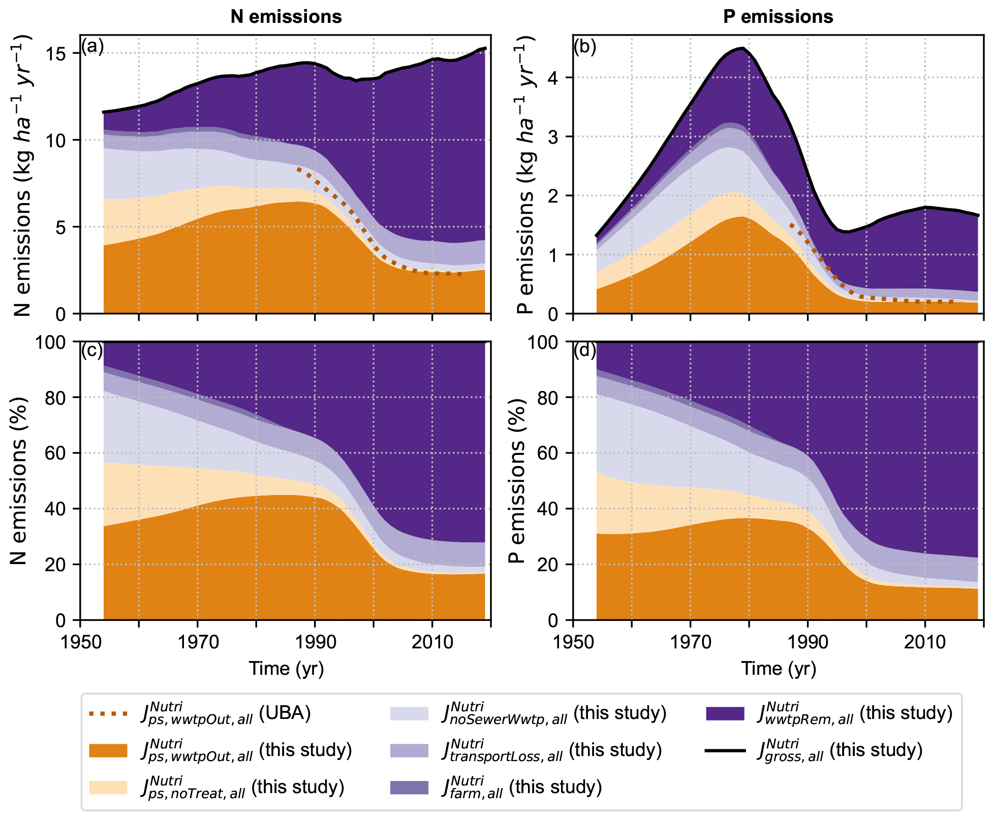
Figure 7 Fate of the N and P gross emissions in Germany at NUTS-0 level for the period 1954–2019 from the mean of our posterior realisations (black line and shaded areas in panels a and b) and independent estimates of WWTP outgoing loads provided by the German Environmental Agency (UBA, 2020) for the period 1987–2016 (dotted red line). All fluxes are shown are 5-year backward-moving averages (the value in 1954 corresponds to the average of the values for 1950–1954). Panels (a) and (c) represent N emissions and panels (b) and (d) P emissions. Panels (c) and (d) report the N and P emissions normalised by the N and P gross emissions, respectively, while panels (a) and (b) show the absolute emissions. The pathways of the gross emissions are point sources (red colours) or other pathways (purple colours). $J_{\mathrm{gross},\mathrm{all}}^{\mathrm{Nutri}}$ denotes the N (Nutri = N) and P (Nutri = P) gross emissions, $J_{\mathrm{ps},\mathrm{wwtpOut},\mathrm{all}}^{\mathrm{Nutri}}$ the N and P WWTP outgoing emissions (treated point sources), $J_{\mathrm{ps},\mathrm{noTreat},\mathrm{all}}^{\mathrm{Nutri}}$ the N and P emissions collected in the public sewer system that are not treated in WWTPs (untreated point sources), $J_{\mathrm{noSewerWwtp},\mathrm{all}}^{\mathrm{Nutri}}$ the N and P gross emissions that are not collected in the sewer system nor treated in WWTPs, $J_{\mathrm{transportLoss},\mathrm{all}}^{\mathrm{Nutri}}$ the N and P emissions lost during wastewater collection and transport, $J_{\mathrm{farm},\mathrm{all}}^{\mathrm{Nutri}}$ the N and P emissions applied to agricultural soils in sewage farms, and $J_{\mathrm{wwtpRem},\mathrm{all}}^{\mathrm{Nutri}}$ the N and P emissions that are removed during treatment in WWTPs. © Authors 2024. This figure is distributed under a CC BY-NC-SA 4.0 licence.

The relative importance of the different P emission pathways (Fig. 7d) follows similar developments to the N emission pathways (Fig. 7c). We note that the contribution of the P point sources, and more specifically the treated component ($J_{\mathrm{ps},\mathrm{wwtpOut},\mathrm{all}}^{\mathrm{P}}$), tends to be lower than that of the N point sources. This can be explained by the higher efficiency of P treatment on average (see efficiency of primary treatment in Table 1 and of secondary and tertiary treatment in Table 5). Unlike the N emissions, the dynamics of the P emission pathways are more governed by the very strong dynamics of the P gross emissions over the period 1950–2019 (Fig. 7b). P gross emissions more than triple between 1950–1954, with an average value of 1.32 kg ha⁻¹ yr⁻¹, and 1974–1979, with an average value of 4.5 kg ha⁻¹ yr⁻¹. The P gross emissions then sharply decrease to achieve about their early 1950s value on average over the period 1992–1996 (1.39 kg ha⁻¹ yr⁻¹) and slightly increase again over the recent period, reaching 1.66 kg ha⁻¹ yr⁻¹ over 2014–2019. While N gross emissions only depend on population dynamics (Supplement Fig. S8) and protein supply per capita (Fig. 3a), P emissions dynamics are driven by the marked development of the P detergents (Fig. 3b–d). P point sources amount to 0.70 kg ha⁻¹ yr⁻¹ on average over 1950–1954 (53.1 % of total emissions) and then increase to reach their maximum value over 1973–1978 equal to 2.06 kg ha⁻¹ yr⁻¹ (46 % of total emissions). They then undergo an almost 10-fold decrease to reach 0.22 kg ha⁻¹ yr⁻¹ over 2000–2004 (13.5 % of total emissions), due to both a drop in detergent use and improvement in wastewater treatment. Similar to N point sources, P point sources are relatively constant over the recent period and amount to 0.19 kg ha⁻¹ yr⁻¹ on average during 2015–2019 (11.6 % of total emissions). Since the N and P point sources have different temporal dynamics, their N:P ratio strongly varies in time, namely between 3.5 and 17, and lies around 13.5 on average over the recent period, 2015–2019 (see Supplement Fig. S40).

At NUTS-1 (state) level, the N and P point sources follow temporal developments similar to those at NUTS-0 (Germany) level in general, although differences are observed in their magnitude, for instance, regarding the treated component shown in Figs. 5 and 6. The point sources for the recent period (average 2015–2019), and more specifically the treated component (as the untreated component is negligible for most states), vary in the range 0.4–29.3 kg ha⁻¹ yr⁻¹ for N and 0.04–1.37 kg ha⁻¹ yr⁻¹ for P. The highest values above 10 kg ha⁻¹ yr⁻¹ for N and 0.5 kg ha⁻¹ yr⁻¹ for P are reached in the city states of Hamburg, Bremen, and Berlin (Figs. 5–6b, d, k) that also have the highest population density (Fig. 2). The lowest values below 1 kg ha⁻¹ yr⁻¹ for N and 0.1 kg ha⁻¹ yr⁻¹ for P are found in the states of Lower Saxony, Mecklenburg-Western Pomerania, and Saxony-Anhalt (Figs. 5–6c, m, o), which are also among the states with the lowest population density below two people per hectare for the recent period, 2015–2019 (Fig. 2). The treated point sources are also low in Thuringia, but the untreated point sources are large compared to the other states, namely 0.95 kg ha⁻¹ yr⁻¹ for N and 0.1 kg ha⁻¹ yr⁻¹ for P, resulting overall in a moderate amount of the two point sources (1.8 kg ha⁻¹ yr⁻¹ for N and 0.2 kg ha⁻¹ yr⁻¹ for P). Not only does the magnitude of the pathways of the N and P gross emissions differ between NUTS-1 regions but also the relative proportions of these pathways. Remarkably, the point source contributions to the total emissions vary in rather wide ranges between NUTS-1 regions, for instance between 29.7 % and 63.1 % and between 19.0 % and 62.7 % in 1986–1990 for N and P, respectively, and between 9.3 % and 24.5 % and between 3.3 % and 20.8 % in 2015–2019 for N and P, respectively.

We also observe differences between the NUTS-1 regions of (former) West and East Germany (Supplement Figs. S41–S45). Specifically, the contribution (in %) of the emissions that are not collected in the sewer system nor treated in WWTPs ($J_{\mathrm{noSewerWwtp},\mathrm{all}}^{\mathrm{Nutri}}$) and the untreated point sources ($J_{\mathrm{ps},\mathrm{noTreat},\mathrm{all}}^{\mathrm{Nutri}}$) are always larger on average over the NUTS-1 regions of East Germany. The contribution of the removal in WWTPs ($J_{\mathrm{wwtpRem},\mathrm{all}}^{\mathrm{Nutri}}$) is larger on average over the NUTS-1 regions of West Germany. In Berlin, we observe different dynamics of the N and P emissions compared to the other states. This is because sewage farms were an important pathway prior to 1982 (Fig. 4k), and a time-varying fraction of the population of Berlin is connected to WWTPs located in the neighbouring state of Brandenburg. For instance, we observe a sharp increase in the treated N and P emissions (Figs. 5–6k) in the 1980s, resulting from the discontinuation of the sewage farm operations.

Herein we report the emissions based on the mean estimates of the posterior ensemble. Variations in the magnitude of the N and P emissions occur across the different posterior realisations. In particular, for some NUTS-1 regions, the uncertainty bounds of the different emission pathways show some overlap, which impacts to some degree their relative importance (Figs. S47–48). Nevertheless, the relative importance of the different N and P emission pathways at NUTS-0 level is rather robust against uncertainty (Fig. S46).

5.3 Gridded point source estimates and their uncertainty due to the spatial disaggregation scheme

Figure 8a presents the gridded map of the total N point sources normalised by the total grid cell area ($J_{\mathrm{ps},\mathrm{tot},\mathrm{all}}^{\mathrm{N}}$ (kg ha⁻¹ yr⁻¹)) from the mean of the posterior realisations, which are averaged over the decade 1970–1979 and downscaled using population data only (as detailed in Sect. 2.2). The spatial distribution of $J_{\mathrm{ps},\mathrm{tot},\mathrm{all}}^{\mathrm{N}}$ is strongly influenced by the distribution of the urban and rural population density (Supplement Fig. S5). The densely populated urban areas stand out by their high values of the point sources, shown in red colours. More specifically, we distinguish between the city states of Berlin, Bremen, and Hamburg (denoted as BE, HB, and HH, respectively), as well as areas in the southern to central areas of West Germany that are within the European Megalopolis (so-called “Blue Banana” or “Liverpool–Milan Axis”). In contrast, Fig. 8d shows that as much as 42 % of the grid cells have a small value of the point sources lower than 0.5 kg ha⁻¹ yr⁻¹ (dark-blue colour), due in particular to the very limited generation of N point sources from the rural population that is largely not connected to the sewer system and WWTPs (details in Fig. S23). An exception is the southern to central areas of West Germany, where many cells display light-blue colours, showing a higher contribution of the rural population to the N emissions.

The pattern evolves in time towards a more scattered distribution of the N point sources due to a progressively higher connection of the rural population to the sewer system and WWTPs (Fig. 8b, c, e, f). Notably, the percentage of grid cells with a small value of the point sources lower than 0.5 kg ha⁻¹ yr⁻¹ (dark-blue colour) drops to 18 % in the 1990–1999 decade (Fig. 8e). This percentage however increased again after the 1990s, and it reached 28 % in the 2010–2019 decade. This can be explained by the overall reduction in the N point sources after 1990 due to improvement in wastewater treatment (Sect. 5.2 and Fig. 7). In this regard, we also observe a reduction in the number of grid cells with large values of $J_{\mathrm{ps},\mathrm{tot},\mathrm{all}}^{\mathrm{N}}$ with time. Specifically, the percentage of grid cells with values of the load higher than 5 kg ha⁻¹ yr⁻¹ (red colours) decreases from 32 % over 1970–1979 to 22.5 % over 1990–1999 and 10 % over 2010–2019 (Fig. 8d–f). The temporal changes are also influenced by the local population dynamics (Fig. S6). For example the decreases in N point sources between 1990–1999 and 2010–2019 due to improvement in the wastewater handling system are exacerbated by a reduction in population density in some urban areas in the NUTS-1 region of North Rhine-Westphalia (denoted as NW in Fig. 8a).

The gridded maps of the total N point sources that are downscaled using WWTP data for the treated part (Fig. 8g–i) report large differences in the spatial distributions compared to the maps that are downscaled based on population data only (Fig. 8a–c). The uncertainty in the spatial pattern at grid level due to the choice of the disaggregation scheme tends to increases with time. This is in particular because the importance of the untreated part of the point sources, which is downscaled using population data, reduces with time (Sect. 5.2, Fig. 7). Using WWTP data for disaggregation results in the concentration of the point sources in as few grid cells where WWTPs are located (Fig. 8j–l). These cells can have very high values of the load (dark-red colours) up to 53 252, 36 320, and 15 270 kg ha⁻¹ yr⁻¹ in 1970–1979, 1990–1999, and 2010–2019, respectively. In contrast, the number of grid cells with values of the load lower than 0.5 kg ha⁻¹ yr⁻¹ (dark blue) is large, namely 59 %, 85 %, and 92 % of total grid cells in 1970–1979, 1990–1999, and 2010–2019, respectively (Fig. 8j–l). Consequently, the densely populated urban areas are less visible from Fig. 8g–i, which appear to be more patchy than Fig. 8a–c.

Similar observations can be drawn from the gridded maps of the total P point sources (Supplement Fig. S62). Nonetheless, the temporal evolution of the P point sources differs from that of the N point sources because they are highly influenced by the dynamics of the P detergents (Sect. 5.2, Fig. 7). In this regard, the gridded maps of the P point sources for the decade 1970–1979 show much higher values of the load compared to the maps for the following decades.

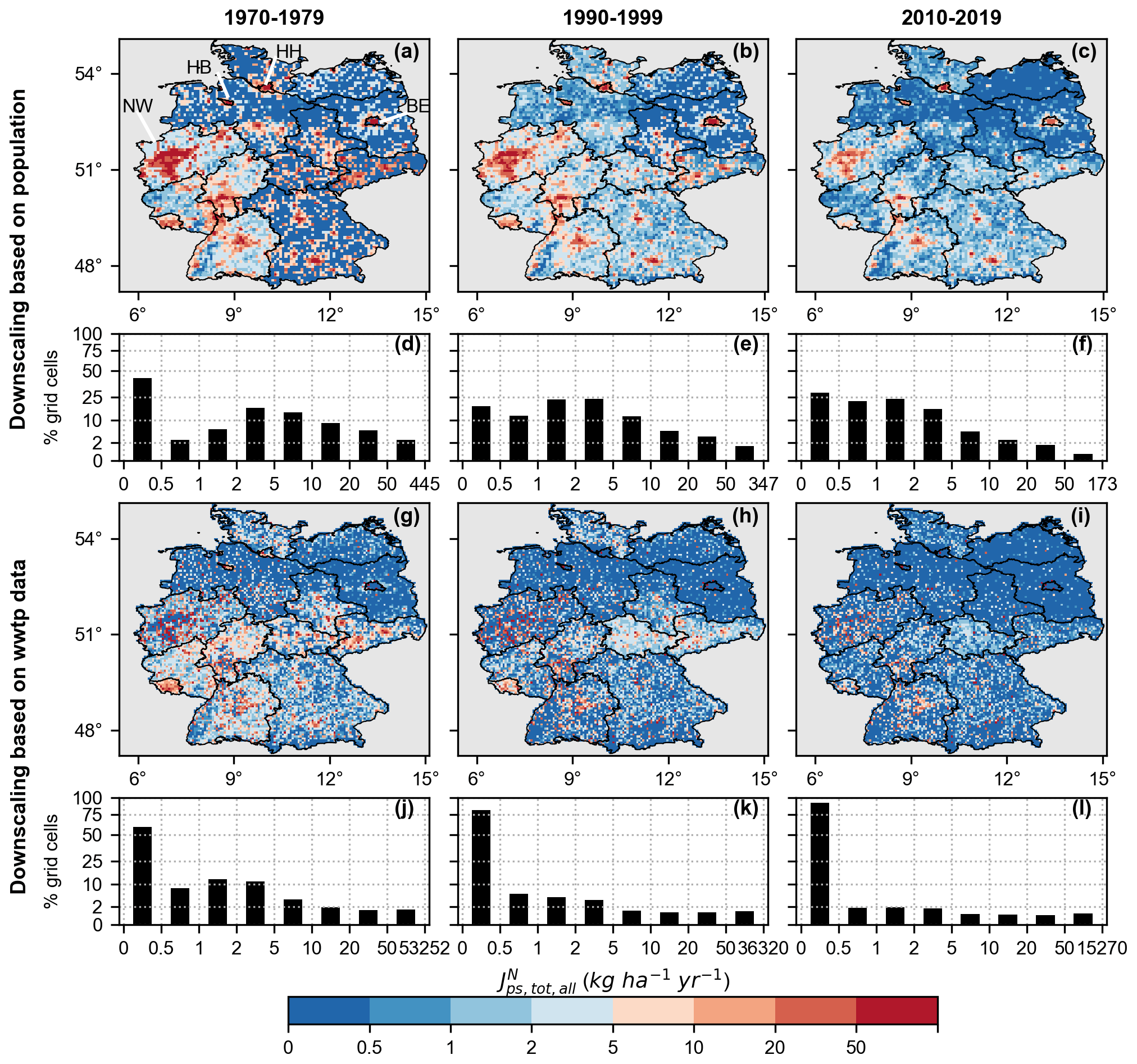
Figure 8 Gridded maps of total N point sources $J_{\mathrm{ps},\mathrm{tot},\mathrm{all}}^{\mathrm{N}}$ in kg ha⁻¹ yr⁻¹ (a–c and g–i), including both the treated and untreated components, and distribution of the grid cell values of $J_{\mathrm{ps},\mathrm{tot},\mathrm{all}}^{\mathrm{N}}$ (d–f and j–l), obtained by downscaling the mean of the posterior realisations from NUTS-1 to grid level using population data (a–f) and WWTP data for the treated component (g–l). The untreated component is always downscaled based on population data. The figure provides the average values in our posterior ensemble over three different decades: 1970–1979 (left panels), 1990–1999 (middle panels), and 2010–2019 (right panels). Panels (a)–(c) show the data at a resolution of 0.015625°, while panels (g)–(i) report aggregated values at a resolution of 0.0625° for depiction purpose (the maps at 0.015625° resolution are reported in Fig S63). Panels (d)–(f) and (j)–(l) all refer to the distribution of the grid cells values at 0.015625° resolution. In all panels, the values of $J_{\mathrm{ps},\mathrm{tot},\mathrm{all}}^{\mathrm{N}}$ were grouped into the same eight classes. The last class of values (depicted in dark-red colour in the maps) includes all values higher than 50 kg ha⁻¹ yr⁻¹. The figure also reports the boundaries of the 16 NUTS-1 units of Germany and indicates the location of the city states, that is Berlin (BE), Bremen (HB), Hamburg (HH), and North Rhine-Westphalia (NW). P point sources are shown in the Supplement, Fig. S62. Data source: the NUTS-1 map comes from the German Federal Agency for Cartography and Geodesy (BKG, 2020) © GeoBasis-DE/BKG dl-de/by-2-0 licence (https://www.govdata.de/dl-de/by-2-0, last access: 21 September 2024). The map is shown in the WGS84 system in the figure. © Authors 2024. This figure is distributed under a CC BY-NC-SA 4.0 licence.

5.4 Uncertainty in point source estimates at river basin level due to the spatial disaggregation scheme

Given the substantial uncertainties in the spatial pattern of the point sources at high spatial resolution (grid level, Sect. 5.3), we examine the uncertainties in the point source estimates at river basin level, which is of interest to water quality studies, as further discussed in Sect. 6.1. We aggregate our gridded point source estimates over a large sample of basins from the HydroBASINS v1.c of the HydroSHEDS database (HydroSHEDS, 2014; Lehner and Grill, 2013). Basins are selected by intersecting all basins of all levels provided by the HydroSHEDS database over Germany and removing duplicates. We also discard small basins that have an area of less than 10 km², which is comparable to the original resolution of the HYDE population dataset (${\mathrm{5}}^{\prime }\times {\mathrm{5}}^{\prime }$) that we use to disaggregate the data from NUTS-1 to grid level. This results in a total of 3778 basins (Fig. 9a), with an area between 10 and 263 580 km². Half of the basins have an area between 114 and 253 km² (25 % and 75 % percentile, respectively), while 5.4 % of the basins have an area higher than 1000 km² (see Fig. S65).

We first analyse the uncertainties in the total N point sources ($J_{\mathrm{ps},\mathrm{tot},\mathrm{all}}^{\mathrm{N}}$ (kg ha⁻¹ yr⁻¹)) for six exemplary nested sub-basins of the Weser River basin, which is Germany's largest national river basin. The sub-basin sizes vary between 210 and 44 949 km², and their extent is shown by the grey-shaded areas in Fig. 9a–b. The temporal variations in the N point sources posterior ensembles are comparable to those observed at NUTS-0 and NUTS-1 level (Sect. 5.2, Fig. 7) for both downscaling schemes, that is the scheme based on population data (shown in green colours) and WWTP data (red colours) (Fig. 9d–h). An exception is the smallest sub-basin (Fig. 9c) that has singular temporal dynamics. The value of the N point sources downscaled based on population data is equal to 0 before 1970. This is because the population in the basin is exclusively rural. Before 1970, the basin did not have point source contributions because rural population is not connected to the sewer system nor to WWTPs.

Figure 9c–h also report the uncertainty due to the choice of the disaggregation scheme with dashed purple lines, which represent the absolute differences between the two means of the posterior ensemble resulting from the two downscaling schemes (solid dark-green and red lines), denoted as $\mathrm{\Delta }\stackrel{\mathrm{‾}}{J_{\mathrm{ps},\mathrm{tot},\mathrm{all}}^{\mathrm{N}}}$. For the basins of intermediate sizes (482–16 097 km²; panels d–g), the absolute differences in the mean tend to first increase with time up to the 1970s–1980s on average between 1.0 and 1.4 kg ha⁻¹ yr⁻¹ and then decline to reach a value between 0.09 and 0.4 kg ha⁻¹ yr⁻¹ on average over the decade 2010–2019. For the smallest (panel c) and largest (panel h) basins, $\mathrm{\Delta }\stackrel{\mathrm{‾}}{J_{\mathrm{ps},\mathrm{tot},\mathrm{all}}^{\mathrm{N}}}$ takes small values (lower than 0.3 kg ha⁻¹ yr⁻¹). Notably, the absolute and relative (normalised by the average values between the two means, Supplement Fig. S71) differences between the means tend to decrease with the basin size for the basins of intermediate to larger sizes (panels e–h).

Figure 9 N point sources ($J_{\mathrm{ps},\mathrm{tot},\mathrm{all}}^{\mathrm{N}}$ in kg ha⁻¹ yr⁻¹) and absolute differences in the mean of the posterior ensemble between the two downscaling approaches based on population and WWTP data ($\mathrm{\Delta }\stackrel{\mathrm{‾}}{J_{\mathrm{ps},\mathrm{tot},\mathrm{all}}^{\mathrm{N}}}$ in kg ha⁻¹ yr⁻¹), aggregated at basins level for river basins of the HydroSHEDS database. Panels (a)–(b) report the map of the 3778 basins selected over Germany, including six exemplary nested sub-basins of the Weser River basin reported in grey-shaded areas. Panels (c)–(h) represent the N point sources for the six sub-basins of the Weser River basin. The light-green-shaded and red-shaded areas delineate the minimum and maximum values over the 100 posterior realisations for the downscaling approach for the treated component based on population and WWTP data, respectively. The solid dark-green and red lines represent the mean of the posterior realisations, and the absolute difference between these two means is shown as dashed purple lines (secondary y axis). Panels (i)–(k) report the distribution (median, interquartile range (IQR), 90 % confidence interval (CI), and full range) of the difference in the means ($\mathrm{\Delta }\stackrel{\mathrm{‾}}{J_{\mathrm{ps},\mathrm{tot},\mathrm{all}}^{\mathrm{N}}}$) against the basin area, which is grouped into 10 classes. The class centres are reported as dark-blue circles along the median line. Distributions are shown for the decades 1970–1979 (i), 1990–1999 (j), and 2010–2019 (k). Data source: basin boundaries come from the HydroBASINS v1.c of the HydroSHEDS database (HydroSHEDS, 2014; Lehner and Grill, 2013) © HydroSHEDS. The map is shown in the WGS84 system in the figure. © Authors 2024. This figure is distributed under a CC BY-NC-SA 4.0 licence.

Figure 9i–k summarise the results regarding the absolute differences in the two means ($\mathrm{\Delta }\stackrel{\mathrm{‾}}{J_{\mathrm{ps},\mathrm{tot},\mathrm{all}}^{\mathrm{N}}}$) for all 3778 selected HydroSHEDS basins. Results are grouped into 10 classes of values according to the basin area and for three time periods, namely 1970–1979 (panel i), 1990–1999 (panel j), and 2010–2019 (panel k). The median value (solid dark-blue line) depicts the overall trend in the absolute difference and shows that $\mathrm{\Delta }\stackrel{\mathrm{‾}}{J_{\mathrm{ps},\mathrm{tot},\mathrm{all}}^{\mathrm{N}}}$ tends to decrease with the basin area and with time. In particular, in the 1970–1979 decade (panel i), the median is decreasing from 3–4 kg ha⁻¹ yr⁻¹ for basin areas lower than 100 km² (two left-most dark-blue circles in panel i) to around 1.2 kg ha⁻¹ yr⁻¹ for basin areas around 1000 km² (fifth dark-blue circles from the left in panel i) and to 0.07–0.42 for basin areas higher than 10 000 km² (three right-most circles in panel i). In the 2010–2019 decade (panel k), the median is equal to 1–1.5, 0.4, and 0.04–0.07 kg ha⁻¹ yr⁻¹ for basin areas lower than 100 km², around 1000 km², and higher than 10 000 km², respectively. The median of the relative differences (expressed in %; Supplement Fig. S71) also tends to decrease with the basin area. Relative differences are however more stable with time, apart from basins with an areas lower than 100 km² for which it tends to increase with time.

The width of the different envelops depicted in Fig. 9i–k (interquartile range, 90 % confidence interval and full range) represents the variability in the absolute differences across basins given the basin size. All envelop widths tend to decrease with time and with the basin size, as the disaggregation of the point sources over smaller basins is influenced by the local specificity, while larger basins capture larger-scale tendencies. For smaller basin sizes, the width of the 90 % confidence interval and the full range take very high values up to 90 and 3038 kg ha⁻¹ yr⁻¹ (left-most area class in panel i). In contrast, the 90 % confidence interval and the full range are of limited magnitude for larger catchments and are always lower than 1.5 kg ha⁻¹ yr⁻¹ for basin areas higher than 10 000 km². A similar tendency is found for the relative differences (Supplement Fig. S71).

Further details on the absolute and relative differences for all decades in the period 1950–2019 are reported in the Supplement, Figs. S66 and S67. The uncertainty in the P point source estimates at river basin level due to the spatial disaggregation scheme shows similar patterns to those of uncertainty in the N point source estimates (Figs. S68–S70 and S72 in the Supplement).

6 Use of the point source dataset and future perspectives

6.1 Value and potential use of the dataset

Our N and P point source dataset builds upon a diverse set of information. In particular, we collect Germany-specific detergent data from the German Federal Ministry of the Environment, Nature Conservation and Nuclear Safety (BMU) and the German Cosmetic, Toiletry, Perfumery and Detergent Association (IKW), which reflect legislation changes over the period 1975–2019. Instead, previous studies rely on proxy data (GDP) for the estimate of detergent use (Van Drecht et al., 2009; Morée et al., 2013) and on large-scale detergent datasets that have a limited temporal extent (1985–2000) (Grizzetti et al., 2022; Vigiak et al., 2023).

We incorporate in our modelling approach observational data of the treated part of the N and P point sources, that is the WWTP outgoing load (1) at NUTS-1 level, for which data are available over a time period starting between 1987 and 2008 depending on the NUTS-1 regions and ending in general in 2019 and that are used for parameter estimation and model evaluation, and (2) at WWTP level, for which data are representative of the period around the year 2016 and that are used for downscaling the treated point source estimates. We could thus verify the plausibility of our N and P point source estimates at NUTS-1 level that capture the WWTP outgoing load observations and additional observational data of WWTP incoming load reasonably well (Sect. 5.1). The performances are lower with respect to WWTP incoming P emissions. Not only could this be due to inaccuracies in our realisations but also to uncertainties in the observational data, which consist of measurements, as well as possibly estimated values when observations are not available, as reported in Sect. 3.5.2.

Importantly, our dataset goes beyond these WWTP observational data, by systematically providing long-term (1950–2019) and high-resolution (0.015625° grid) point sources, including both the part which is treated in WWTP and the part which is not treated and directly discharged into surface waters from the sewer system. In this regard, the dataset accounts for the large temporal changes in the N and P point sources and their N:P ratio (Sect. 5.2). Temporal dynamics are strongly influenced by the 1991 Urban Waste Water Treatment Directive (EC, 1991), which led to an improvement in wastewater treatment and a large decrease in N and P point sources in the 1990s and the 1980 Phosphate Ordinance (PHochstMengV, 1980) and the subsequent self-commitment of the laundry detergent manufacturers to produce phosphate-free detergents, which resulted in a sharp reduction in detergent phosphate in the 1980s and early 1990s. It is also crucial to consider the point sources that are not treated in WWTP and for which no observational data are available. In fact, they contribute substantially to the total point sources before 1990 and over the entire 1950–2019 period for the state of Thuringia.

Such a long-term dataset can support water quality assessment studies. This is demonstrated for example in Nguyen et al. (2022) and Sarrazin et al. (2022) that investigated the N legacies in the soil and groundwater for a large sample of river basins in Germany over the period 1950–2014 and 1960–2015, respectively, using a preliminary version of the N point source dataset presented in this paper (based on NUTS-0 level statistics). In particular, Sarrazin et al. (2022) found that N point sources can have a large impact on the magnitude and trend of the in-stream nitrate concentration in the Weser River basin, since point sources immediately reach surface waters without prior degradation and transport through the soil and groundwater, which happened to the diffuse sources. Our dataset complements existing datasets, not only on point sources for Germany or at a larger-scale (Morée et al., 2013; UBA, 2020; Vigiak et al., 2020, 2023) but also on diffuse sources (Batool et al., 2022; Ebeling et al., 2022; Häußermann et al., 2020), which are also an important source for nutrient pollution. Our database also complements datasets focusing on other aspects of wastewater, such as the global datasets of Ehalt Macedo et al. (2022) on WWTPs location and characteristics and of Jones et al. (2021) on wastewater volume and its pathways, both being limited to the year 2015.

Another important feature of our dataset is that it quantifies uncertainties due to (1) the parameter values (coefficients), including 100 point source estimates that are most consistent with observations at NUTS-1 level, and (2) the downscaling scheme, providing two gridded point sources maps for each of the 100 realisations using population or WWTP spatial data. This results in a total of 200 gridded point source realisations that capture the uncertainties that are due to the paucity of data to constrain the parameters at NUTS-1 level, as well as the lack of spatially resolved data for spatial disaggregation to grid level.

The uncertainties tend to decrease with time. In particular, the parametric uncertainty is lower over the recent period compared to the earlier period where no observations are available to constrain the model parameters (Sect. 5.1). Regarding the downscaling, while the difference between the point source estimates resulting from the two spatial disaggregation scheme reduces with time in absolute terms, it does not vary substantially in relative terms, apart from smaller aggregation scales (basins with area lower than 100 km²), where it even increases with time depending on the local specificity (Sect. 5.4). Importantly, the disaggregation scheme based on WWTP data around the year 2016 produces more accurate results over the recent period than the other scheme. In earlier years, both approaches could be considered to be equiprobable, since they are both based on strong assumptions, namely that the WWTP setting did not change with time (scheme based on WWTP data) and that population density can be an adequate proxy for the spatial distribution of WWTP outgoing emissions (scheme based on population data that was also adopted in previous studies such as Morée et al., 2013, and Vigiak et al., 2023). Therefore, we encourage users of this dataset to devise a time-varying weighting scheme to take into account the varying accuracy in the spatial disaggregation approaches. Such a weighting scheme could ensure that only the estimates downscaled using WWTP data are considered for the recent period, while the uncertainties arising from both downscaling schemes are considered for earlier years. We provide an illustration of such a scheme in the Supplement, Fig. S73. Moreover, the uncertainties in our estimates decrease from grid level (Fig. 8) towards larger spatial aggregation units (e.g. river basins in Fig. 9). In particular, for earlier years, using the data at larger spatial scales of aggregation (above 100 km²) is more reliable given the differences between the two downscaling schemes. Therefore, using the dataset directly at grid level (Sect. 5.3) may be prone to large uncertainties, and our analysis at river basin level (Sect. 5.4) allows reflection on suitable spatial aggregation scales for water quality studies. In this respect, our gridded dataset provides the flexibility to aggregate the point source estimates at any spatial level of interest. Our uncertainty characterisation goes beyond the study of Morée et al. (2013) that analysed the uncertainties in the model coefficients using spatially uniform a priori ranges that were not constrained using observational data as in this study. Nonetheless, Morée et al. (2013) also found a tendency toward higher uncertainties in the past compared to the more recent period.

Overall, the point source data for the past period have to be interpreted as providing temporal and spatial trends rather than precise estimates. A reason for this is the use of qualitative and proxy information, not only to downscale the data to grid level but also to derive the point source estimates at NUTS-0 and NUTS-1 level in the absence of quantitative data, in particular for the period before the 1990s for East Germany, before the 1980s for West Germany, and for the entire period 1950–2019 for industrial and commercial emissions. A comparison of our data with independent estimates provided by the German Environmental Agency for the period 1987–2016 (UBA, 2020) indeed shows a good consistency in the temporal trends, with increasing similarity between the two datasets with time (Sect. 5.1).

6.2 Directions for future improvement of the dataset

The point source dataset presented in this paper accounts for N and P emissions from wastewater that are collected by the sewer system and/or treated in urban WWTPs, resulting from human excreta, detergent P use, and industrial indirect emissions. The incorporation of additional point source constituents in future versions of this dataset would provide a more comprehensive database for N and P point source emissions. One of the main constituents to be addressed is the industrial direct emissions. These emissions are difficult to estimate due to a lack of data, and it may only be possible to recover a lower bound for these emissions from the available data (such as the E-PRTR and IED records), as discussed in the Introduction (Sect. 1). However, given their importance in magnitude, industrial direct emissions and their uncertainties would be worth further investigation in future studies. In this respect, the NUTS-0 level dataset of the German Environmental Agency (UBA, 2020) indicates that the ratio of industrial direct emissions to WWTP outgoing emissions over the period 1983–1987 is as much as 40 % for N and 12 % for P. This ratio decreases with time to reach 12 % for N and 4 % for P over the period 2012–2016, but, as mentioned earlier, this is likely to be a lower bound.

Urban runoff that is collected in the sewer system (storm sewers or combined sewers) can also lead to large N and P loads being discharged to surface waters because, on the one hand, it contains N and P in particular due to atmospheric N and P deposition (Yang and Toor, 2018). On the other hand, when collected in combined sewer systems that also carry wastewater, urban runoff can cause combined sewer overflow (CSO), when the capacity of the effluent handling system is exceeded during storm events (Fuchs et al., 2010; Pistocchi et al., 2019). This results in wastewater being discharged directly to surface waters without treatment in WWTPs. Urban runoff and CSO have been identified as important sources of pollution to be addressed in the revision of the Urban Waste Water Treatment Directive, which is currently in preparation (Vikolainen, 2023). However, the magnitudes of storm sewer N and P discharge and CSO are uncertain, since no observational data are currently available, and their estimation involves simplifying assumptions and uncertain coefficients (Fuchs et al., 2010; Pistocchi et al., 2019).

Another potentially important contributor to point sources is the domestic emissions that are not connected to the sewer system nor to WWTPs via transport from cesspits. While these emissions are overall of limited importance in the recent period, their magnitude is large in the earlier period (Sect. 5.2). It would therefore be critical to elucidate their fate in Germany and in other countries where these emissions can be substantial for the recent period as well (Vigiak et al., 2020). These emissions are handled in particular in septic tanks or independent wastewater systems (Vigiak et al., 2020, 2023). They could be either a diffuse source to soils or a point source to surface waters, as documented for example in MUGV (2010) for the recent period in Germany. Due to a lack of detailed information on these emissions, previous studies made simplifying assumptions. In Germany, Fuchs et al. (2010) consider that disconnected population is equipped with septic tanks from which a part of the N and P is transported to WWTPs, while the other part is a diffuse source. In Europe, Grizzetti et al. (2022) and Vigiak et al. (2020) consider that it is entirely a diffuse source and that N and P are reduced with the same efficiency as that of primary treatment (Vigiak et al., 2020) or possibly secondary treatment (Grizzetti et al., 2022). Globally, Morée et al. (2013) and Van Puijenbroek et al. (2019) consider that the urine part is a point source, while the feces part is a diffuse source. Other point source constituents can also contribute to the total point sources, such as intensive livestock operations and fish farms. However, to our knowledge, these emissions were not considered in previous point source assessment in Europe.

Moreover, our dataset can be further improved by explicitly accounting for N emissions embedded in food waste disposal in sewers. This can be considered the same way as in the recent IPCC (2019) report using a coefficient that represents the ratio of protein disposed of via this route to total human N excreta, and it is suggested to be 1.09 in Europe. The estimation of this coefficient is however highly uncertain due to a lack of reporting datasets. In Germany, food disposal down the drain could account for overall 14 % of the domestic food waste (Schmidt et al., 2019). However, this figure cannot be related to the amount of protein wasted, due to a lack of information regarding the specific food commodities involved. Here, we argue that, by considering a large uncertainty range in the fraction of protein supply wasted at the distribution and consumption level ($f_{\mathrm{waste}}^{\mathrm{pro}}$; see Table 1), we may implicitly account for the fact that part of the protein wasted may actually contribute to the point sources.

As in previous point source estimates (Morée et al., 2013; Van Drecht et al., 2009; UBA, 2020; Vigiak et al., 2020, 2023), our dataset does not distinguish between the different N and P species that constitute wastewater and that can have a different impact on the environment. For instance, nitrogen can be present as ammonia (NH₃), which is very toxic for aquatic ecosystem, or as ammonium (NH${}_{\mathrm{4}}^{+}$) or nitrate (NO${}_{\mathrm{3}}^{-}$), which are less toxic (Camargo and Alonso, 2006). In this respect, future studies could quantify the proportions of these different N species in point sources. For this, further data on population connection to advanced (tertiary) wastewater treatment could be collected, to account not only for treatment with targeted denitrification as in this study but also for treatment with targeted nitrification, which is the transformation from NH₃ to N0${}_{\mathrm{3}}^{-}$. Some data are provided, for instance, by the Statistical Office of Germany (SO-DE, 1975–2007, 2010–2022).

Overall, we propose that future water quality studies could perform sensitivity analysis to better understand the impact of different possible assumptions on the N and P pathways discussed in this section. For Germany, such investigation is facilitated as we provide all data that we produced, along with our model code (see “Code and data availability” section).

7 Code and data availability

The dataset (version 1.1) is available from a Zenodo repository at https://doi.org/10.5281/zenodo.10500535 (Sarrazin et al., 2024). It includes (1) the input and calibration data at NUTS-1 level (CSV files); (2) the input data at grid level (netCDF files); (3) the 200 gridded (0.015625° resolution) N and P point source estimates, resulting from the 100 posterior parameter sets and the two spatial disaggregation schemes (netCDF files); (4) the 100 NUTS-1 level estimates of N and P gross emissions and their different pathways from the 100 posterior parameter sets (CSV files); and (5) the 200 basin-level N and P point source estimates for each of the 3778 basins selected from the HydroSHEDS database (CSV files). The code of the N and P point sources model is written in Python and is available from a GitHub repository (https://github.com/fannysarrazin/NP_point_sources_model, last access: 15 January 2024); it has been assigned a DOI (https://doi.org/10.5281/zenodo.10501238; Sarrazin and Kumar, 2024).

8 Conclusions

The main features of the N and P point source dataset introduced in this paper are that it provides long-term (1950–2019) and high-resolution (0.015625°) estimates for Germany, not only of the domestic and industrial point sources that are treated in urban WWTPs but also of the untreated domestic point sources that are collected in the sewer system, while considering the uncertainties in modelling choices (i.e. coefficients and downscaling approaches). Our data construction is the result of a substantial data collection from a multitude of different sources to extract state-level or at least country-specific data, wherever possible.

Overall, the magnitude of the N and P point sources strongly varies in time and space, and we recommend that they should be careful examined in water quality studies. Despite the uncertainties involved in point source estimation and the fact that not all point source constituents are included in this version of the dataset (e.g. industry direct emissions), we believe that this dataset supports robust long-term water quality and nutrient assessment studies. In fact, we provide 200 realisations of the point sources, in an attempt to characterise their uncertainties, and a detailed discussion on how to interpret these estimates and to best use them, given their level of precision that varies in time and across spatial aggregation scales. In addition, we provide a transparent methodology that builds on existing modelling concepts to enable long-term reconstruction, while incorporating observational WWTP load data, to increase the accuracy and precision of the estimates. A similar approach could be adopted by other researchers to develop other national and regional datasets where sub-national and observational point source datasets are available. This would contribute to improve our large-scale understanding of nutrient point sources and their impact on the (aquatic) environment.