A field-based thickness measurement dataset of fallout pyroclastic deposits in the peri-volcanic areas of Campania (Italy): statistical combination of different predictions for spatial estimation of thickness

Determining the spatial thickness (z) of in situ and reworked fallout pyroclastic deposits plays a key role in volcanological studies and in shedding light on geomorphological and hydrogeological processes in peri-volcanic areas. However, this is a challenging line of research because (1) field-based measurements are expensive and time-consuming, (2) the ash might have been dispersed in the atmosphere by several volcanic eruptions, and (3) wind characteristics during an eruptive event and soil-forming and/or denudation processes after ash deposition on the ground surface affect the expected spatial distribution of these deposits. This article tries to bridge this knowledge gap by applying statistical techniques for making representative spatial thickness predictions to be used for the analysis of geomorphic processes at the catchment and sub-catchment scales. First, we compiled a field-based thickness measurement dataset (https://doi.org/10.5281/zenodo.8399487; Matano et al., 2023) of fallout pyroclastic deposits in the territories of several municipalities in Campania, southern Italy. Second, 18 predictor variables were derived mainly from digital elevation models and satellite images and were assigned to each measurement point. Third, the stepwise regression (STPW) model and random forest (RF) machine learning technique are used for thickness modeling. Fourth, the estimations are compared with those of three models that already exist in the literature. Finally, the statistical combination of different predictions is implemented to develop a less biased model for estimating pyroclastic thickness. The results show that the prediction accuracy of RF (RMSE <82.46 and MAE <48.36) is better than that of existing models in the literature. Moreover, statistical combination of the predictions obtained from the above-mentioned models through a least absolute deviation (LAD) combination approach leads to the most representative thickness estimation (MAE <45.12) in the study area. The maps for the values estimated by RF and LAD (as the best single model and combination approach, respectively) illustrate that the spatial patterns did not change significantly, but the estimations by LAD are smaller. This combined approach can help in estimating the thickness of fallout pyroclastic deposits in other volcanic regions and in managing geohazards in areas covered with loose pyroclastic materials.

1 Introduction

A significant quantity of ash is dispersed in the atmosphere during an explosive volcanic eruption and is deposited over a large area of ground surface following wind transportation. The spatial thickness of the ash layer typically decreases with distance from the eruptive vent (e.g., see Perrotta and Scarpati, 2003; Bourne et al., 2010; Lowe, 2011; Brown et al., 2012; Caron et al., 2012; Costa et al., 2012; Albert et al., 2019; Eychenne and Engwell, 2023) and noticeably influences geomorphological and hydrological processes such as landscape evolution, hillslope hydrology, erosion, and slope stability because the geotechnical and hydraulic properties of the unconsolidated ash layer usually differ from the underlying bedrock and soil. A deep understanding of the thickness of fallout pyroclastic deposits could, therefore, help address geohazard management and many related socioeconomic concerns. It is challenging to estimate the spatial thickness of fallout pyroclastic deposits because there might be more than one eruptive event, the ash dispersal pattern is influenced by the changes in wind characteristics (e.g., the speed and direction of the wind) during a single eruption, and soil-forming and denudation processes continuously influence the expected spatial thickness due to different slope exposures and geometry. Only costly and time-consuming detailed field-based measurements may allow us to effectively map the thickness variations of fallout pyroclastic deposits over a limited area (for examples, see Matano et al., 2016; Cuomo et al., 2021). The spatial thickness of fallout pyroclastic deposits under the influence of hillslope processes, accordingly, remains a knowledge gap (P. De Vita et al., 2006).

Estimating the residual regolith has been a common practice (e.g., Saulnier et al., 1997; Saco et al., 2006; Tesfa et al., 2009; Segoni et al., 2013), and the implemented models performed better when developed based on independent variables and when applied to a specific site or in limited areas (Del Soldato et al., 2018; Matano et al., 2016). Conventional approaches for predicting pyroclastic thickness primarily rely on geological data, but the significant improvements in the availability of remote sensing data, along with the recent advances in recording the depositional history of fallout pyroclastic deposits, present a unique opportunity to enhance prediction accuracy. Moreover, the statistical literature shows that better results can be achieved by combining estimations derived from different models, which has not been adopted for the objectives of this article to date.

This article explores the integration of a wide range of predictor variables, mainly derived from digital elevation model (DEM) and satellite multispectral images, with machine learning techniques (i.e., stepwise regression and random forest). These approaches identify the most relevant variables and capture non-linear relationships between the predictor variables and pyroclastic thickness values in order to improve prediction accuracy. Combination schemes were then applied to the predictions of these methods and to the ones derived from classical approaches, as slope angle pyroclastic thickness (SAPT; P. De Vita et al., 2006), geomorphological pyroclastic thickness (GPT; Del Soldato et al., 2016), and slope exponential pyroclastic thickness (SEPT; Del Soldato et al., 2018) methods. Finally, the predictions are validated by field-based measurements of fallout pyroclastic deposits to empirically demonstrate that combining the results of different models provides better thickness predictions for the fallout pyroclastic deposits.

The different sections of this article are briefly introduced here to provide better insight into content of this article. Section 2 introduces the study area, while Sect. 3 explains the data collection in the field, along with the methodology for preparing the predictor variables and for predicting the thickness of fallout pyroclastic deposits. In the next section, a detailed description of the field-based thickness measurement dataset and of the predictor variables is provided. Section 5 discusses the results and highlights the advantages of using statistical combination in predicting the thickness of fallout pyroclastic deposits. The concluding remarks and suggestions for future work are presented in the last section.

2 Study area

The area of interest encompasses Campania and the immediate surroundings in southern Italy (Fig. 1). It is bounded on the west by the Tyrrhenian Sea and on the east by the Apennine hilly–mountainous inner land, with an altitude of up to 2050 m a.s.l. at Mt. Miletto. The area has a Mediterranean climate with hot, dry summers and moderately cool rainy winters. The mean annual temperature is about 10 °C in the mountainous areas and roughly 18 °C along the coast. The mean annual rainfall ranges from 700 mm in the eastern part of the region to 1800 mm in the central part of the Apennine mountains (Ducci and Tranfaglia, 2008).

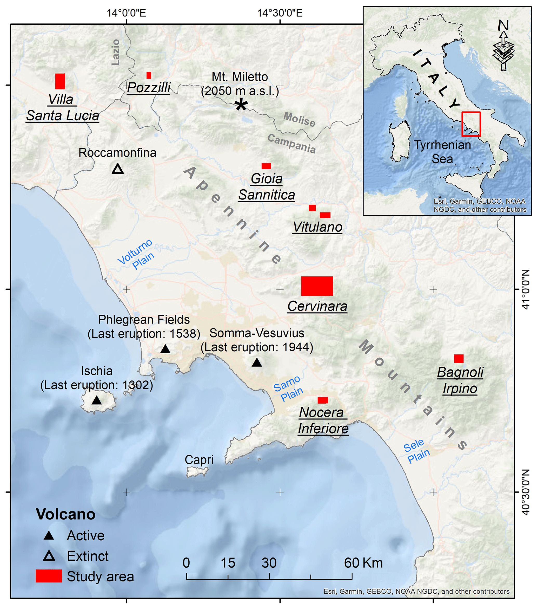
Figure 1 Location of the study area in southern Italy.

The geological units of the Apennine mountains are formed by Triassic to Early Miocene carbonate platform limestones and pelagic basin calcareous pelitic sequences. They are strongly deformed, mainly thrusted eastward (Bonardi et al., 2009; Doglioni, 1991; Patacca et al., 1990) and uncomformably covered by Middle Miocene to Pliocene thrust-top basin fillings, formed by siliciclastic sequences (mostly clay, sandstone, and conglomerate; Di Nocera et al., 2006).

The Quaternary extension in the hinterland and the axial sectors of Campania caused several fluvio-lacustrine intramontane-basin openings (Ferranti and Oldow, 2005; Amato et al., 2018; Boncio et al., 2022). The NW–SE- and NE–SW-striking faults delimit the strongly subsiding coastal basins (e.g., Volturno, Campania, Sarno, and Sele plains) along the Tyrrhenian belt where the volcanic complexes of Somma–Vesuvius, Phlegrean Fields, Ischia, and Roccamonfina occur (Fig. 1). The volcanoes are active (except for Roccamonfina) and have erupted at least once in the last 1000 years (Rosi and Sbrana, 1987; Santacroce, 1987). Diffuse degassing, fumaroles, and hot springs are observed around and in the submerged sectors of the volcanoes (Rosi and Sbrana, 1987; Chiodini et al., 2001; de Lorenzo et al., 2001). The above-mentioned volcanic complexes are briefly introduced below:

• The Somma–Vesuvius volcanic complex lies over a large sedimentary plain, prevalently filled by pyroclastic deposits. In this volcanic complex, the older Mt. Somma stratovolcano was cut by an eccentric polyphasic caldera and by the Vesuvius stratocone (Sbrana et al., 2020). Four main Plinian eruptions (Cioni et al., 2003; Santacroce et al., 2008; Sulpizio et al., 2010a, b; Mele et al., 2011; Sevink et al., 2011; Doronzo et al., 2022) and several interplinian eruptions (Andronico and Cioni, 2002; Cioni et al., 2015; Sulpizio et al., 2005, 2007; Bertagnini et al., 2006) have been linked to the volcanic activities of Somma–Vesuvius.

• The Phlegrean Fields consist of several volcanoes in a large caldera west of Naples, characterized by many eruptions with a large and very large volcanic explosivity index (VEI; Newhall and Self, 1982) (Fig. 2). Volcanic activity in the Phlegrean Fields began prior to 80 ka (Pappalardo et al., 1999; Scarpati et al., 2014), and the caldera collapses occurred during the eruptions of Campanian Ignimbrite (ca. 39 ka; Deino et al., 2004; De Vivo et al., 2001), Masseria del Monte Tuff (29 ka; Albert et al., 2019), and Neapolitan Yellow Tuff (15 ka; Orsi et al., 1996; Perrotta et al., 2006; Vitale and Isaia, 2014). The post-15 ka activity was well described by Di Vito et al. (1999), Isaia et al. (2009), and Smith et al. (2011).

• Ischia Island is the emergent part of a volcanic edifice in the Gulf of Naples, whose activity started before 150 ka. The island is composed of volcanic rocks (mostly trachyte and phonolite) formed by effusive and explosive eruptions, epiclastic deposits, and subordinate terrigenous sediments (S. De Vita et al., 2006).

• The Roccamonfina volcanic complex was active between 550 and 150 ka in the Garigliano River rift valley. It was affected by an intense Plinian activity revealed by very large craters. The central caldera is the result of the eruptive explosions at 353 ± 5 ka, while the latest stage of activity featured the edification of the central shoshonitic domes at 150 ka (Giannetti, 2001; Rouchon et al., 2008).

The fallout pyroclastic deposits considered in this article are mainly related to the Somma–Vesuvius and Phlegrean Fields volcanoes (Fig. 2) because the thickness of the Ischia tephra is not considerable on the mainland, and the old Roccamonfina deposits have mostly eroded outside the volcanic edifice. Therefore, only the volcanic history of Somma–Vesuvius and Phlegrean Fields will be further described in this section.

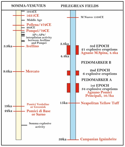
Figure 2 Main explosive eruptions of the Somma–Vesuvius and Phlegrean Fields volcanoes. The major explosive events are in red. The pedomarker A and the pedomarker B refer to paleosol layers developed during eruptive quiescence.

2.1 The volcanic history of the Phlegrean Fields

The most important volcanic activities in the Phlegrean Fields are the Campanian Ignimbrite (CI: 39 ka; De Vivo et al., 2001) and the Neapolitan Yellow Tuff eruptions (15 ka; Orsi et al., 1992, 1996; Wohletz et al., 1995; Deino et al., 2004). The former is the most powerful volcanic event to have ever occurred in the Mediterranean area (Barberi et al., 1978; Fisher et al., 1993; Orsi et al., 1996; Rosi et al., 1988, 1996; Civetta et al., 1997; De Vivo et al., 2001; Cappelletti et al., 2003; Engwell et al., 2014; Scarpati and Perrotta, 2016; Smith et al., 2016) and emplaced thick sequences of fallout deposits and pyroclastic density currents of mostly trachytic composition (Giaccio et al., 2008; Costa et al., 2022). The dispersed ash during the first eruptive phase was transported by wind towards the east (Rosi et al., 1999; Perrotta and Scarpati, 2003; Scarpati and Perrotta, 2016). The pyroclastic density currents were subsequently emplaced over an area of 7000 km² and surmounted ridges more than 1000 m high (Barberi et al., 1978; Fisher et al., 1993). The CI distal outcrops are mostly represented by a massive, gray ignimbrite (Barberi et al., 1978; Fisher et al., 1993; Scarpati et al., 2014), distributed beyond ∼ 80 km from the vent (Smith et al., 2016).

The post-15 ka activity of the Phlegrean Fields was concentrated in three epochs separated by two quiescent periods (Fig. 2; Di Vito et al., 1999; Smith et al., 2011; Di Renzo et al., 2011, and references therein) and terminated with the Monte Nuovo eruption in 1538 CE (Guidoboni and Ciuccarelli, 2011; Di Vito et al., 2016, and references therein). The first epoch (15 to ∼ 9.5 ka) was characterized by several explosive events, of which the Pomici Principali eruption was the most energetic (Lirer et al., 1987; Di Vito et al., 1999). This epoch was followed by a quiescent period when a thick paleosol layer, pedomarker A, was developed. The second epoch (8.6–8.2 ka; Di Vito et al., 1999) was distinguished by only a few episodes of low-magnitude eruptions, mainly in the NE Campanian Plain. After formation of the pedomarker B in a prolonged volcanic quiescence, the last epoch of intense volcanic activity began between 4.4 and 3.8 ka (Di Vito et al., 1999). The third epoch was characterized by several explosive events, of which the Agnano–Monte Spina eruption (4.4 ka; De Vita et al., 1999; Dellino et al., 2021) was the most powerful. This epoch was followed by a prolongate quiescent period and then the Monte Nuovo eruption (1538 CE; Di Vito et al., 1987; Piochi et al., 2005). Since 1960, fumarolic and hydrothermal activities with episodes of bradyseism have mainly occurred in the Phlegrean Fields (Cannatelli et al., 2020).

2.2 The volcanic history of Somma–Vesuvius

The Somma–Vesuvius volcanic activity is characterized by four major Plinian eruptions (i.e., Pomici di Base or “Sarno” at ca. 22 ka, Mercato or “Ottaviano” at ca. 9.0 ka, Avellino at 3.9 ka, and Pompeii at 79 CE) and several low-intensity interplinian eruptions (Fig. 2). Pomici di Base (Andronico et al., 1995; Santacroce et al., 2008) was the oldest caldera-forming event, which was followed by notably variable interplinian activities, alternating low-magnitude eccentric flank eruptions, quiescent phases, and subplinian events (such as the Greenish Pumice eruption at ∼ 19 ka; Santacroce and Sbrana, 2003; Santacroce et al., 2008). The products of the Mercato eruption (Rolandi et al., 1993a; Mele et al., 2011) that occurred about 13,000 years later were separated from those of the Avellino eruption (Rolandi et al., 1993b; Sulpizio et al., 2010a, b; Sevink et al., 2011) by a thick paleosol layer (Di Vito et al., 1999). The low-intensity eruptions of AP1–AP6 (3.5–2.3 ka; Andronico et al., 2002; Santacroce et al., 2008; Passariello et al., 1999, 2010; Di Vito et al., 2019) preceded the eruption of Pompeii, which has been well described by many authors (from Sigurdsson et al., 1985, to Doronzo et al., 2022, and references therein).

The Vesuvius cone was formed by the most recent period of volcanic activity, characterized by a complex alternation of periods of activity with various explosive characters and quiescent phases (Andronico et al., 1995) suddenly interrupted by the Pollena eruption (472 CE; Rolandi et al., 2004). A Middle Age period of variable activity was then started, with alternating lava effusions, moderately explosive eruptions, and mild periods (Rolandi et al., 1998), before a subplinian eruption in 1631 CE (Bertagnini et al., 2006). After this event, the volcano entered a state of semi-persistent mild activity, with minor lava effusions and short quiescent periods. Each period of repose was preceded by relatively powerful explosive and effusive polyphase eruptions (Arrighi et al., 2001), like the last two in 1908 and 1944.

3 Materials and methods

The data and methods used in this study are summarized in Table 2 and Fig. 3 and are further described in this section.

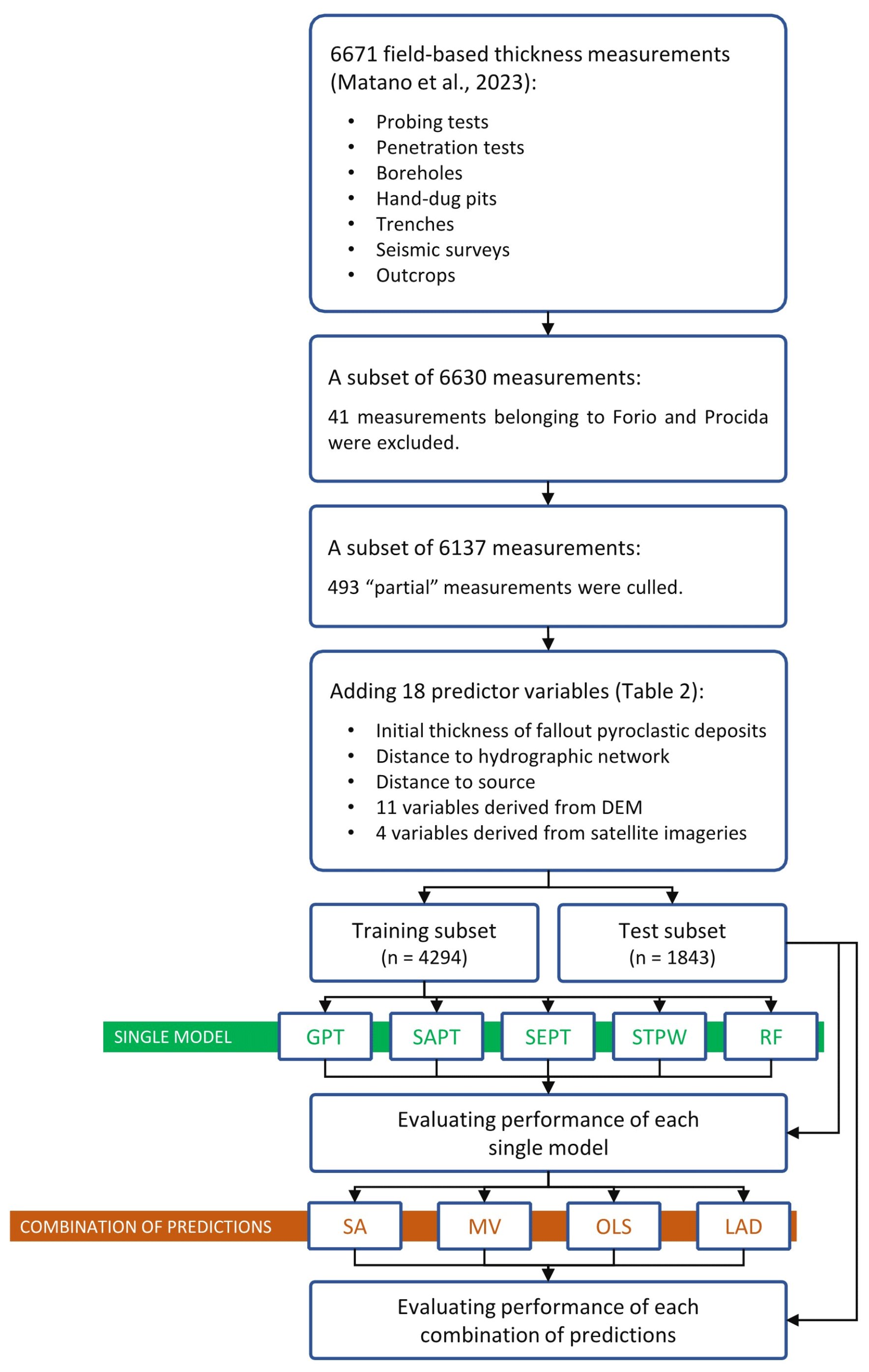
Figure 3 A flowchart showing how the dataset of field-based thickness measurements (Matano et al., 2023) is used to predict the thickness of the fallout pyroclastic deposits. GPT: geomorphological pyroclastic thickness, SAPT: slope angle pyroclastic thickness, SEPT: slope exponential pyroclastic thickness, STPW: stepwise regression, RF: random forest, SA: simple average, MV: minimum variance, OLS: ordinary least squares, LAD: least absolute deviation.

3.1 Dataset of field-based thickness measurements

A dataset of 6671 field-based thickness measurements (Matano et al., 2023) has been collected during the field surveys and investigations conducted over the last few decades for scientific and technical studies in the study area (Fig. 1). The measurements explain the distance between the topographic surface and the upper limit of the consolidated basement; we refer to “total” measurement when the instruments could measure the whole distance and “partial” measurement when the limitations of the implemented instruments led to only partial measurements of the distance. Further details about the stratigraphy of the pyroclastic deposits and the possible presence of non-lithified paleosols are not considered as they are beyond the scope of this article. The following methods have been applied for measuring the thickness of the unconsolidated pyroclastic materials on the bedrock:

• Probing tests (PRBs). An iron rod (1.8 cm in diameter and up to 306 cm in length) was driven into the ground by hand or by a 0.03 kN hammer to measure the depth of the underlying consolidated bedrock, indicating the thickness of the fallout pyroclastic deposits as well. Each measurement represents the arithmetic mean of two or three measured values within a circle with a radius of 1–2 m to minimize the error associated with the local factors such as the presence of cobbles, boulders, roots, colluvium, and pumice layers.

• Penetration tests. Two types of penetration tests were implemented in this study. The dynamic cone penetration tests (DPT–DL030) were performed by driving an iron rod with a cross-sectional area of 10 cm² into the ground by repeatedly raising a 0.3 kN weight for 20 cm and then dropping it. These tests refer to the in situ continuous measurement of rock and/or soil resistance to penetration up to 14 m depth, which could also be an indirect measure for the thickness of the fallout pyroclastic deposits when the probe fails to penetrate. The data collected by this method are in accordance with the probing-test results and help interpret the stratigraphy as well. We also used the results of the standard penetration test (SPT), which is a common in situ dynamic test for determining the geotechnical properties of subsurface soil such as relative density and shear strength parameters.

• Boreholes (BHs). The borehole stratigraphic data were used for collecting the thickness of fallout pyroclastic deposits.

• Hand-dug pits (HDPs). These were usually excavated manually (mainly at a size of 20 × 20 × 200 cm) near penetration test or geophysical survey sites to collect further information on the stratigraphy of the loose materials over the bedrock.

• Trenches (TRNs). These were excavated (1 m wide, 3 m long, and 2–3 m deep) at the base of the slopes or along the intermediate morphological shelves using mechanical diggers for direct investigation of the pyroclastic-deposit stratigraphy.

• Seismic surveys (SSs). Up to 10 m depth, the seismic reflection data of three bursts (direct, reverse, and intermediate) were recorded by 20–24 geophones placed 3–5 m apart in a straight line on the ground surface. The seismic data revealed the geometry and stratigraphy of the ash layer, along with the boundary between the consolidated bedrock and the overlying loose materials.

• Outcrops (OCPs). The stratigraphy of several outcrops was analyzed across the study area to measure the thickness of the pyroclastic deposits.

For each method, the measurement error and estimated interpretation uncertainty (i.e., estimation of the fallout pyroclastic-deposit thickness) are shown in Table 1. About 1 cm error is expected for direct thickness measurements conducted with outcrops, hand-dug pits, trenches, and boreholes. The error associated with the probing-test results is around 1 cm as well. The measurement error of the penetration tests (i.e., dynamic cone penetration test (DPT–DL030) and standard penetration test) is considered to be 10 cm because the number of blows was counted following the driving of the rod into the ground for 10 cm. In seismic surveys, the error depends on the specific technique and site characteristics, but a measurement error of 100 cm might be a good estimation for the whole study area.

Table 1 The expected measurement error and interpretation uncertainty for the methods implemented.

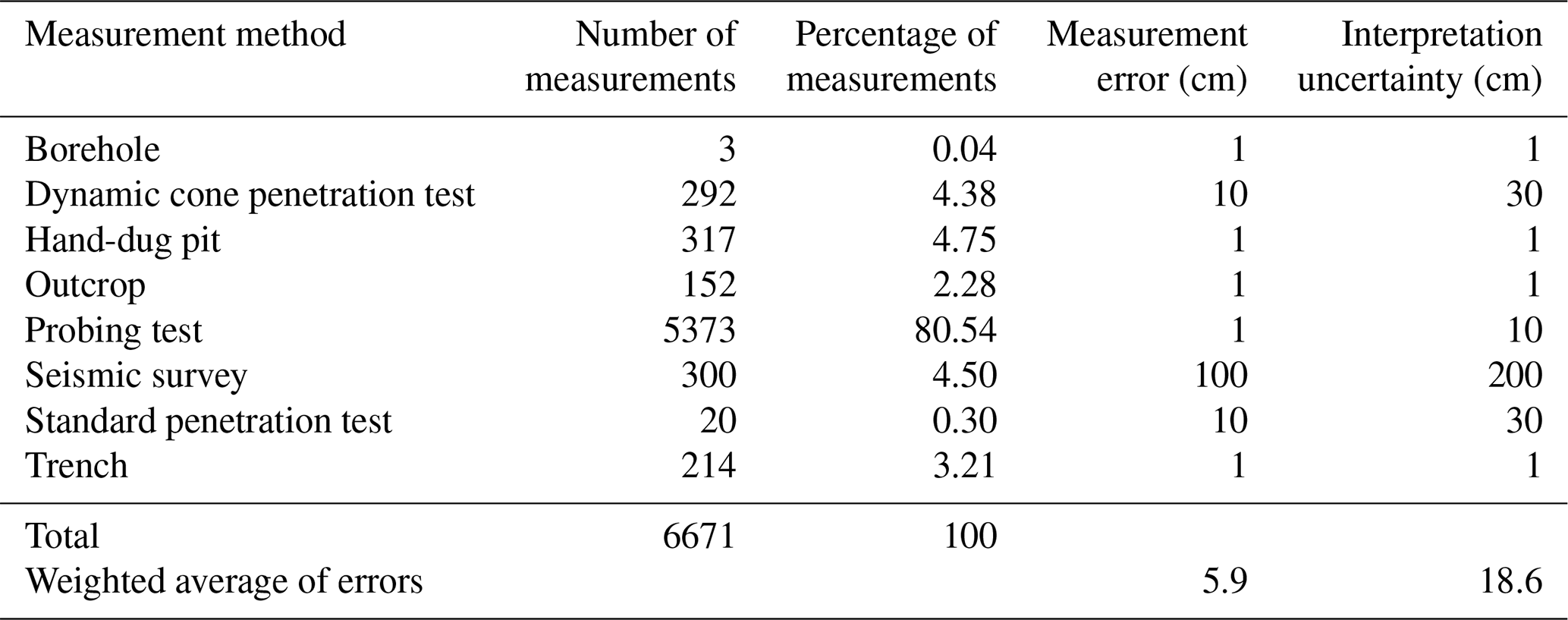
The interpretative uncertainty of the measurements is equal to the measurement error (i.e., 1 cm) for direct thickness measurements, but it increases in probing tests, penetration tests, and seismic surveys. It is noteworthy that the results of these tests and/or surveys were calibrated in the field based on the more precise tests conducted nearby (mostly at 1–10 m distance). The weighted average of errors and the uncertainty are under 6 and 19 cm, respectively (Table 1). Therefore, the bias introduced by measurement errors and interpretative uncertainties is irrelevant to the objectives of this article.

To date, partial and total thickness measurements, the method of investigation, the municipal territory to which the measurement points belong, and the geographic coordinates have been recorded for a total of 6671 points (Matano et al., 2023). The spatial distribution of the measurement points is shown in Fig. 4. Matano et al. (2016) and Cuomo et al. (2021) have already used the measurements in the Cervinara and Nocera Inferiore municipal territories for detailed thickness mapping with heuristic methods.

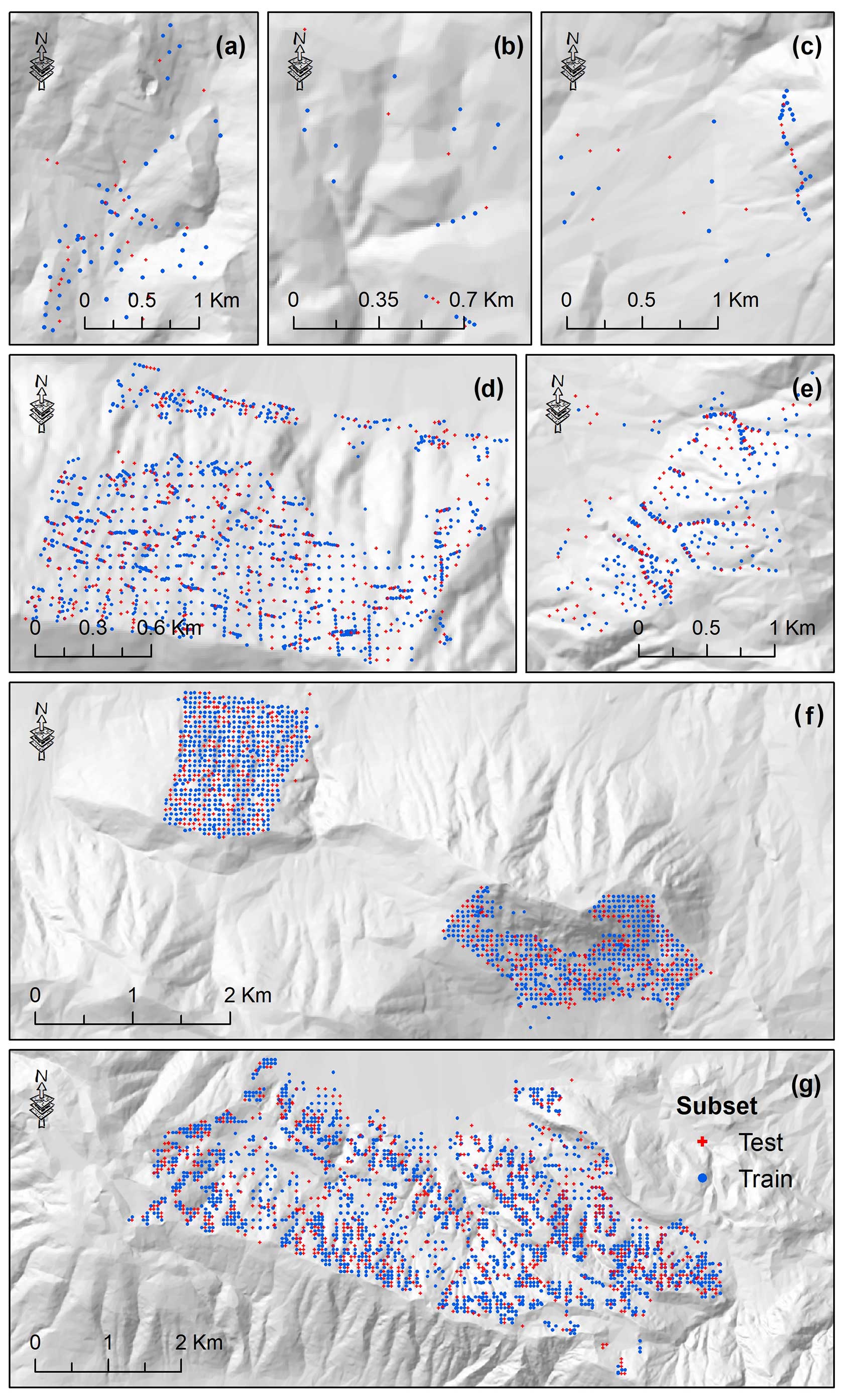
Figure 4 Spatial distribution of field-based thickness measurement points in each municipality: (a) Villa Santa Lucia, (b) Pozzilli, (c) Gioia Sannitica, (d) Nocera Inferiore, (e) Bagnoli Irpino, (f) Vitulano, and (g) Cervinara. The measurement points are subdivided into the training (n=4294) and test (n=1843) subsets. Although symbols of different shapes and colors are used for the subsets, the spatially dense measurement points do not allow for the application of a larger symbol size. In the electronic version of this article, please zoom in on the figure to distinguish between different symbols based on the shape (if required).

3.2 Predictor variables

A list of the potential predictor variables for estimating the thickness of fallout pyroclastic deposits is provided in Table 2. The value for each predictor variable is assigned to the measurement points based on a set of rasters at 30 × 30 m resolution.

Table 2 The predictor variables for thickness modeling.

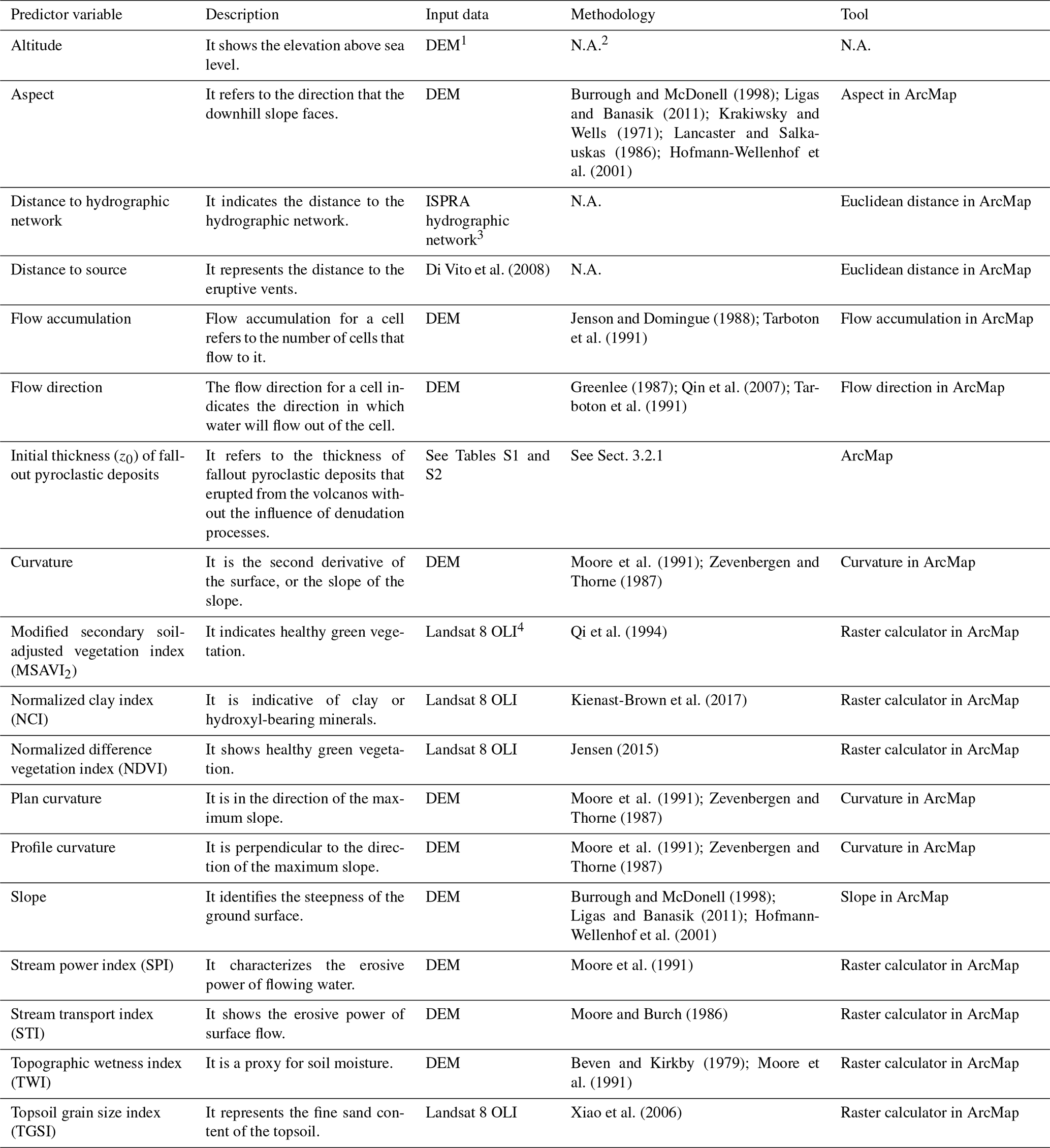
¹ The vertical accuracy of the DEM is evaluated by control points, and the overall root mean square error is <3.5 m (Tarquini et al., 2007). ² Not applicable. ³ https://geodati.gov.it/resource/id/ispra_rm:01Idro250N_DT (last access: 8 January 2024). ⁴ Operational Land Imager. Landsat 8 OLI data are calibrated to better than 5 % uncertainty in terms of the top-of-atmosphere reflectance and have an absolute geodetic accuracy better than 65 m circular error at 90 % confidence (Ihlen, 2019).

3.2.1 Initial thickness (z₀) of fallout pyroclastic deposits

This predictor variable represents the overall thickness of fallout pyroclastic deposits emplaced by Late Quaternary explosive eruptions at a given location. In other words, it explains the thickness value that could be estimated at a location if erosional and/or depositional processes do not occur after the associated eruptive events. In fact, the residual thickness of pyroclastic deposits that can be found at a certain location today is the result of the erosional and depositional processes that occurred after the eruptive events.

To obtain the initial thickness (z₀) of fallout pyroclastic deposits, the following approach is used: (1) collect the isopach maps of the fallout deposits for the main volcanic eruptions (characterized by a high explosivity index and great eruptive volume) in Campania from the literature (Tables S1 and S2 in the Supplement); (2) georeference and digitize each map; (3) apply an interpolation technique (i.e., Topo to Raster in ArcMap) to add intermediate isopaches in case of a significant gap between them; (4) assign the average value of two isopaches of different thickness to the area between them, except for the area enclosed by only one isopach; (5) combine all shapefiles into one; (6) compute the z₀ value of all volcanic eruptions for each feature in the shapefile; and (7) convert the obtained shapefile into a raster with 30 × 30 m resolution and assign the z₀ value to each field-based measurement point in the thickness dataset (Sect. 3.1).

The isopach maps of the fallout deposits for the Somma–Vesuvius and Phlegrean Fields main eruptions are listed in Tables S1 and S2, respectively. The Ischia tephra was not considered for z₀ calculation because of its insignificant thickness on the mainland. However, the old Roccamonfina tephra (>150 ka) has been almost entirely eroded outside the volcanic edifice, and we have considered the associated isopach map of pyroclastic deposits only in a semi-quantitative way based on the results of Rouchon et al. (2008) and Giannetti (2001).

Isopach maps are commonly used in volcanological studies to estimate the volume of a single eruptive event and to assess volcanic hazard. They are constructed by interpolating thickness data points, which are considered to be reliable as they are directly measured by investigating the stratigraphy of volcanic deposits. To the best of our knowledge, the uncertainty of the published isopach maps for Somma–Vesuvius and Phlegrean Fields (De Vita et al., 1999; Di Vito et al., 2008; Cappelletti et al., 2003; Costa et al., 2009; Isaia et al., 2004; Orsi et al., 2004; Rolandi et al., 1998, 2004, 2008) has not been discussed in the literature. Only Costa et al. (2012) modeled the Campanian Ignimbrite isopach map based on 113 measurements and reported that the results are in agreement with the measured thickness values (relative mean error $=\sim \mathrm{0.3}$ log units). The uncertainty has also not been quantified for the cumulative isopach maps of multiple eruptions generated for studying erosional processes and landslide susceptibility (P. De Vita et al., 2006; De Vita and Nappi, 2013; Del Soldato et al., 2016, 2018).

3.2.2 Variables derived from DEM and satellite imagery

The predictor variables derived from DEM or satellite imagery (11 and 4 variables, respectively) are listed in Table 2 with a definition, a brief description, and the methodology used to obtain them. Originally, the DEM had a 10 × 10 m spatial resolution, while the satellite imagery had a 30 × 30 m spatial resolution. Raster resampling is, therefore, implemented after calculating the variables to obtain a resolution of 30 × 30 m.

Other variables such as the distance to the hydrographic network and the distance to the source (i.e., eruptive vent) are also considered to be predictor variables in this study. In the latter, several inferred eruptive vents reported by Di Vito et al. (2008), along with the Vesuvius crater and Roccamonfina caldera, were considered to take into account different ash-producing eruptions and to reduce the associated uncertainty as far as possible. Further information is provided in Table 2.

3.3 Methods for thickness modeling

3.3.1 Previous studies

To date, four approaches have been proposed for modeling the thickness (z) of the fallout pyroclastic deposits. The slope angle pyroclastic thickness (SAPT) model estimates z by linking the initial thickness (z₀) of fallout pyroclastic deposits that have erupted from the volcanos with the slope angle (P. De Vita et al., 2006; De Vita and Nappi, 2013). In this model, some thresholds for slope angle were derived by field measurements in Mt. Sarno and Mt. Lattari. The geomorphologically indexed soil thickness (GIST) model is an empirical model that combines morphometric, geomorphological, and geological features (Catani et al., 2010) for estimating soil thickness in areas where bedrock weathering is the main soil-forming process (Mercogliano et al., 2013; Segoni et al., 2013), but it is applied to the areas covered by the fallout pyroclastic deposits as well (Rossi et al., 2013). In this article, the GIST model was not implemented because the fallout pyroclastic deposits are of allochthonous origin, and bedrock lithology does not control their thickness (P. De Vita et al., 2006; Del Soldato et al., 2018). Del Soldato et al. (2016) proposed the geomorphological pyroclastic thickness (GPT) model as a combination of the SAPT and GIST models. Comparing the performances of the GIST, SAPT, and GPT models indicated that z is mainly controlled by z₀ and slope gradient. Therefore, the slope exponential pyroclastic thickness (SEPT) model was developed based on these two parameters (Del Soldato et al., 2018).

3.3.2 Proposed methods: random forest

For spatial modeling, a wide range of machine learning techniques are available, including logistic regression analysis, random forest (RF), support vector machines, and artificial neural networks. Among these techniques, RF showed the best performance for classification and prediction. It is a shallow ensemble-learning algorithm that can be tuned with few parameters (Liu et al., 2023, and references therein). The principles of decision trees and bagging are implemented for building random forests. Bagging applies bootstrap sampling of the training data for building decision trees and aggregates the predictions across all the trees, which reduces the overall variance and improves the predictive performance. The RF uses a random subset of variables at each split while growing a decision tree during the bagging process to generate a more diverse set of trees, which helps lessen tree correlation beyond bagged trees and noticeably increases the predictive power.

After splitting a given dataset randomly into training and test subsets (Fig. 4), the RF regression modeling could be applied as follows: (1) generate an RF model using the training subset, (2) calculate the variable importance for the established model, (3) apply the constructed RF model to the test subset and evaluate the results, and (4) implement the trained RF model for making predictions in the unknown locations.

The R packages rsample (Frick et al., 2022) and ranger (Wright and Ziegler, 2017) are used for data splitting and modeling, respectively. We considered 70 % of the whole dataset to be the training subset and considered the rest to be the test subset in data splitting (Fig. 4). For training a model, different values are assigned to each hyperparameter, including the number of variables to possibly split at each node (m_try), the minimal node size at which to split (min.node.size), the sample with and without replacement (replace), and the fraction of observations to sample (sample.fraction). A data frame from all possible combinations of m_try, min.node.size, replace, and sample.fraction was then generated; the RF model was trained for each combination; and the best one in terms of root mean square error (RMSE) and mean absolute error (MAE) was selected (see Sect. 3.3.5 for more information). The optimum number of trees (num.trees) was finally investigated by running the RF model for 50 different num.trees values between 0 and 1000. Using the determined hyperparameters, the RF model is trained for making predictions; the performance of the model is evaluated; and the importance of the variables is calculated by (1) the Gini index (Fig. 10b), which indicates the number of times a variable is responsible for a split and the impact of that split divided by the number of trees, and (2) the permutation importance (Fig. 10c), which calculates the prediction accuracy in the out-of-bag observations and recomputes the prediction accuracy after eliminating any association between the variable of interest and the outcome by permuting the values of the variable under evaluation. The difference between the two accuracy values is the permutation importance for the given variable from a single tree. The average of the importance values for all the trees in an RF then gives the RF permutation importance of this variable.

3.3.3 Proposed methods: stepwise regression

Multiple linear regression is used to analyze the relationship between a single response variable (dependent variable) and two or more independent variables (predictor variables). Assuming we store P predictor variables ($p=\mathrm{1},\mathrm{\dots },P$) for N locations ($i=\mathrm{1},\mathrm{\dots },N$) in a matrix X {x_i,p}, we could simply predict the thickness z {z_i} using multiple linear regression:

$$\begin{array}{}\text{(1)}& \mathit{z}=\mathit{\beta }\mathbf{X}+\mathit{\epsilon },\end{array}$$

with $\mathit{\beta }=[{\mathit{\beta }}_{\mathrm{1}},\mathrm{\dots },{\mathit{\beta }}_P{]}^{\prime }$ being the vector of the regression coefficients and ε being a vector of i.i.d. (independent and identically distributed) error terms. However, not all the P variables are necessarily relevant for making predictions, and more accurate predictions may be obtained by a subset $\stackrel{\mathrm{̃}}{\mathbf{X}}\left\{{\stackrel{\mathrm{̃}}{x}}_{i,p},p=\mathrm{1},\mathrm{\dots },\stackrel{\mathrm{̃}}{P};\stackrel{\mathrm{̃}}{P}<P\right\}$ of predictor variables. Then, the final model can be written as follows:

$$\begin{array}{}\text{(2)}& \mathit{z}=\mathit{\delta }\stackrel{\mathrm{̃}}{\mathbf{X}}+\mathit{\eta },\end{array}$$

with $\mathit{\delta }=[{\mathit{\delta }}_{\mathrm{1}},\mathrm{\dots },{\mathit{\delta }}_{\stackrel{\mathrm{̃}}{P}}{]}^{\prime }$ being the vector of the selected best $\stackrel{\mathrm{̃}}{P}<P$ variables and η being the new vector of error terms.

Different methods such as forward selection, backward elimination, and stepwise regression (STPW) are used for this aim. All these methods are based on a series of automated steps (Taylor and Tibshirani, 2015). A forward-selection approach initially assumes no predictor variable and adds the most statistically significant variable, one by one, until no more variables remain. On the contrary, the backward-elimination approach initially includes all predictor variables and then eliminates the least statistically significant variables one by one. However, the STPW method is a combination of forward selection and backward elimination. As with forward selection, the procedure starts with no variables and adds variables using a pre-specified criterion. At every step, the procedure also considers the statistical consequences of dropping the previously included variables. The STPW method is applied in this article with the R package StepReg (Li et al., 2020).

3.3.4 Proposed methods: combination approaches

The RF, STPW, GPT, SAPT, and SEPT models possess their own strengths and weaknesses. Previous studies showed that a combination of the predictions obtained with different methods allows for more accurate estimations (e.g., in the case of time series, see Eliott and Timmermann, 2004; Chan and Pauwels, 2018). Therefore, combination-based predictions are commonly used in many applicative fields (e.g., Cui et al., 2021; Nti et al., 2020; Wong et al., 2007; Yang, 2018).

One of the most common approaches for combining predictions is the stacking ensemble (Ganaie et al., 2022). It trains different models on the same dataset and generates predictions that become the input of a superior model (known as a second-level model; see Ribeiro and dos Santos Coelho, 2020). The fundamental concept behind stacking is that the optimal combination of the predictions of different models achieves better predictive performance compared to those obtained with single models.

Let us define, for each ith location, a vector consisting of $K(k=\mathrm{1},\mathrm{\dots },K)$ alternative predictive models ${\widehat{z}}_i=[{\widehat{z}}_{i,\mathrm{1}}{\widehat{z}}_{i,\mathrm{2}},\mathrm{\dots },{\widehat{z}}_{i,k},\mathrm{\dots },{\widehat{z}}_{i,K}{]}^{\prime }$ which can be obtained considering some inputs as shown in Fig. 4. Then, a final prediction at the ith location can be defined according to

$$\begin{array}{}\text{(3)}& {\stackrel{\mathrm{̃}}{z}}_i=f({\widehat{z}}_i,\mathit{\omega }),\end{array}$$

with $\mathit{\omega }=[{\mathit{\omega }}_{\mathrm{1}},{\mathit{\omega }}_{\mathrm{2}},\mathrm{\dots },{\mathit{\omega }}_k,\mathrm{\dots },{\mathit{\omega }}_K{]}^{\prime }$ being the vector of K weights associated with the K different competing spatial predictive models. In other words, the stacking ensemble ${\stackrel{\mathrm{̃}}{z}}_i$ is a function of the K predictions with different base models for the same location ${\widehat{z}}_i$. In particular, we assume a linear function:

$$\begin{array}{}\text{(4)}& {\stackrel{\mathrm{̃}}{z}}_i={\mathit{\omega }}^{\prime }{\widehat{z}}_i=\sum _{k=\mathrm{1}}^K{\mathit{\omega }}_k{\widehat{z}}_{i,k}.\end{array}$$

In this framework, an important issue is the selection of the combination weights ω. For this aim, we can use subjective or objective weighting systems based on either expert evaluations or some statistical criteria. In this paper, we compare the performance of four objective weighting systems and choose the best one.

As the first approach, we consider the simple average (SA) combination, in which the K competing models are weighted equally; i.e., ${\mathit{\omega }}_{\mathrm{SA}}=[\frac{\mathrm{1}}{K},\mathrm{\dots },\frac{\mathrm{1}}{K}{]}^{\prime }$. Despite its simplicity, this approach empirically provides a better performance compared to more sophisticated alternatives (Hsiao and Wan, 2014). Another commonly adopted approach for the optimal selection of combination weights is based on the variance minimization criterion (MV; see Bates and Granger, 1969; Newbold and Granger, 1974). Given a set of K competing predictive models, the weights are chosen by minimizing the variance of the prediction errors:

$$\begin{array}{}\text{(5)}& \begin{array}{c}min\\ \mathit{\omega }\end{array}{\mathit{\omega }}^{\prime }{\mathbf{\Sigma }}_{\mathrm{e}}\mathit{\omega },\text{with}{\mathit{\iota }}^{\prime }\mathit{\omega }=\mathrm{1},\end{array}$$

with $\mathit{\iota }={\left[\mathrm{1},\mathrm{1},\mathrm{\dots },\mathrm{1}\right]}^{\prime }$ being a vector of ones and Σ_e being the K×K covariance matrix associated with the prediction errors of the K competing models. The optimal solution to this minimization problem is given by

$$\begin{array}{}\text{(6)}& {\mathit{\omega }}_{\mathrm{MV}}={\displaystyle \frac{{\mathbf{\Sigma }}_{\mathrm{e}}^{-\mathrm{1}}\mathit{\iota }}{{\mathit{\iota }}^{\prime }{\mathbf{\Sigma }}_{\mathrm{e}}^{-\mathrm{1}}\mathit{\iota }}},\end{array}$$

where ${\mathbf{\Sigma }}_{\mathrm{e}}^{-\mathrm{1}}$ is the inverse of the covariance matrix, also known as the precision matrix.

The third approach implemented for choosing combination weights ω is based on ordinary least squares (OLS) regression (Granger and Ramanathan, 1984), where ω can be chosen by considering the following linear regression:

$$\begin{array}{}\text{(7)}& z_i={\mathit{\omega }}_{\mathrm{0}}+\sum _{k=\mathrm{1}}^K{\mathit{\omega }}_k{\widehat{z}}_{i,k}+{\mathit{\epsilon }}_i,\end{array}$$

with ω₀ being the constant term, ω_k being the generic kth weight associated with the kth competing model, and ε_i being an i.i.d. error term. According to OLS combination, the weight vector $\mathit{\omega }=[{\mathit{\omega }}_{\mathrm{1}},\mathrm{\dots },{\mathit{\omega }}_K{]}^{\prime }$ is obtained by solving the following minimization problem:

$$\begin{array}{}\text{(8)}& \begin{array}{c}min\\ {\mathit{\omega }}_{\mathrm{1}},\mathrm{\dots },{\mathit{\omega }}_K\end{array}\sum _{i=\mathrm{1}}^N{\left(z_i-\sum _{k=\mathrm{1}}^K{\mathit{\omega }}_k{\widehat{z}}_{i,k}\right)}^{\mathrm{2}}.\end{array}$$

The OLS approach requires computing the weights in a training subset and using the selected ones in a test subset. It has the advantage of generating unbiased combined predictions without the need to investigate the bias for the individual models. This weighting approach is, however, sensitive to outliers. To address this issue, previous studies proposed the least absolute deviation (LAD) combination approach based on the minimization of the absolute loss function (Nowotarski et al., 2014):

$$\begin{array}{}\text{(9)}& \begin{array}{c}min\\ {\mathit{\omega }}_{\mathrm{1}},\mathrm{\dots },{\mathit{\omega }}_K\end{array}\sum _{i=\mathrm{1}}^N\left|z_i-\sum _{k=\mathrm{1}}^K{\mathit{\omega }}_k{\widehat{z}}_{i,k}\right|.\end{array}$$

3.3.5 Accuracy evaluation

To evaluate and compare the performance of the K predictive models and their combinations, the root mean square error (RMSE) and the mean absolute error (MAE) are computed. Let us first define the prediction error e_i,k of the kth model (including combinations of the models) for the observed ith location:

$$\begin{array}{}\text{(10)}& e_{i,k}=z_i-{\widehat{z}}_{i,k}.\end{array}$$

The RMSE_k and MAE_k are defined as follows:

$$\begin{array}{}\text{(11)}& {\displaystyle }{\mathrm{RMSE}}_k=\sqrt{{\displaystyle \frac{\mathrm{1}}{N}}\sum _{i=\mathrm{1}}^N{e}_{i,k}^{\mathrm{2}}}=\sqrt{{\displaystyle \frac{\mathrm{1}}{N}}\sum _{i=\mathrm{1}}^N{\left(z_i-{\widehat{z}}_{i,k}\right)}^{\mathrm{2}}},\text{(12)}& {\displaystyle }{\mathrm{MAE}}_k=\sqrt{{\displaystyle \frac{\mathrm{1}}{N}}\sum _{i=\mathrm{1}}^N\left|e_{i,k}\right|}=\sqrt{{\displaystyle \frac{\mathrm{1}}{N}}\sum _{i=\mathrm{1}}^N\left|z_i-{\widehat{z}}_{i,k}\right|}.\end{array}$$

Notice that the MAE loss is less affected by outliers than RMSE, and we prefer the models with lower MAE in case of ambiguity. The difference in the accuracy of the two competing models might also be due to randomness, especially for small differences. Therefore, several equal predictive accuracy (EPA) tests (Diebold and Mariano, 2002) were used in this article for comparing the K competing models and their combinations and for highlighting the statistically significant improvements in accuracy. Specifically, given two competing models k and k^′, we define a generic loss function g(⋅) of the prediction errors g(e_i,k) and $g\left(e_{i,k^{\prime }}\right)$. In our case, we consider squared and absolute losses (RMSE and MAE, respectively). Let us define the loss differential vector $\mathit{d}=[d_{\mathrm{1}},d_{\mathrm{2}},\mathrm{\dots },d_N{]}^{\prime }$, where, for each generic ith location,

$$\begin{array}{}\text{(13)}& d_i=g\left(e_{i,k}\right)-g\left(e_{i,k^{\prime }}\right).\end{array}$$

Under the null hypothesis, the vector d has zero mean, and the two competing models k and k^′ have the same predictive accuracy. Under the alternative hypothesis, the two models are statistically different, and the best model is the one associated with the lowest statistical loss. In practice, the EPA test can be simply applied by regressing the loss differential vector d with a constant vector ι of ones and by conducting inference with robust standard errors to account for possible heteroskedasticity.

4 Description of the field-based thickness dataset and related predictor variables

We first explain the process of creating a subset from the dataset of Matano et al. (2023) (n=6671) to achieve our research objectives. Briefly, 41 measurements belonging to the Forio and Procida municipalities are excluded because they are not located on the mainland. The subset is populated with 18 predictor variables and is visualized in Figs. 5–8 to give an idea of the available data for detailed elaboration. It is noteworthy that the partial thickness measurements (n=493) are then culled, and the remaining 6137 points (Fig. 2) are considered for thickness modeling in the following section. The field-based thickness measurements range between 0 and 1450 cm. Most of the measurements refer to total thickness, representing the thickness of fallout pyroclastic deposits from the ground surface to the underlying bedrock (Fig. 5). The median of partial thickness values is 3 times greater than that of total thickness (approximately 200 and 60 cm, respectively). This is mainly due to the application of the probing tests and the hand-dug pits in the areas with thick fallout pyroclastic deposits, where the thickness is greater than the maximum survey depth reached by these two measurement methods: 300 and 200 cm respectively. The average and the range of thickness values mainly show the limitations of the measurement methods. The probing test is the leading methodology implemented in field surveys, and the measured values usually range from 10 to 300 cm. The recorded values are often <10 cm in outcrops and 200–800 cm in the measurements conducted with SPT and boreholes. The greatest thickness in the dataset is determined by seismic surveys (Fig. 5d).

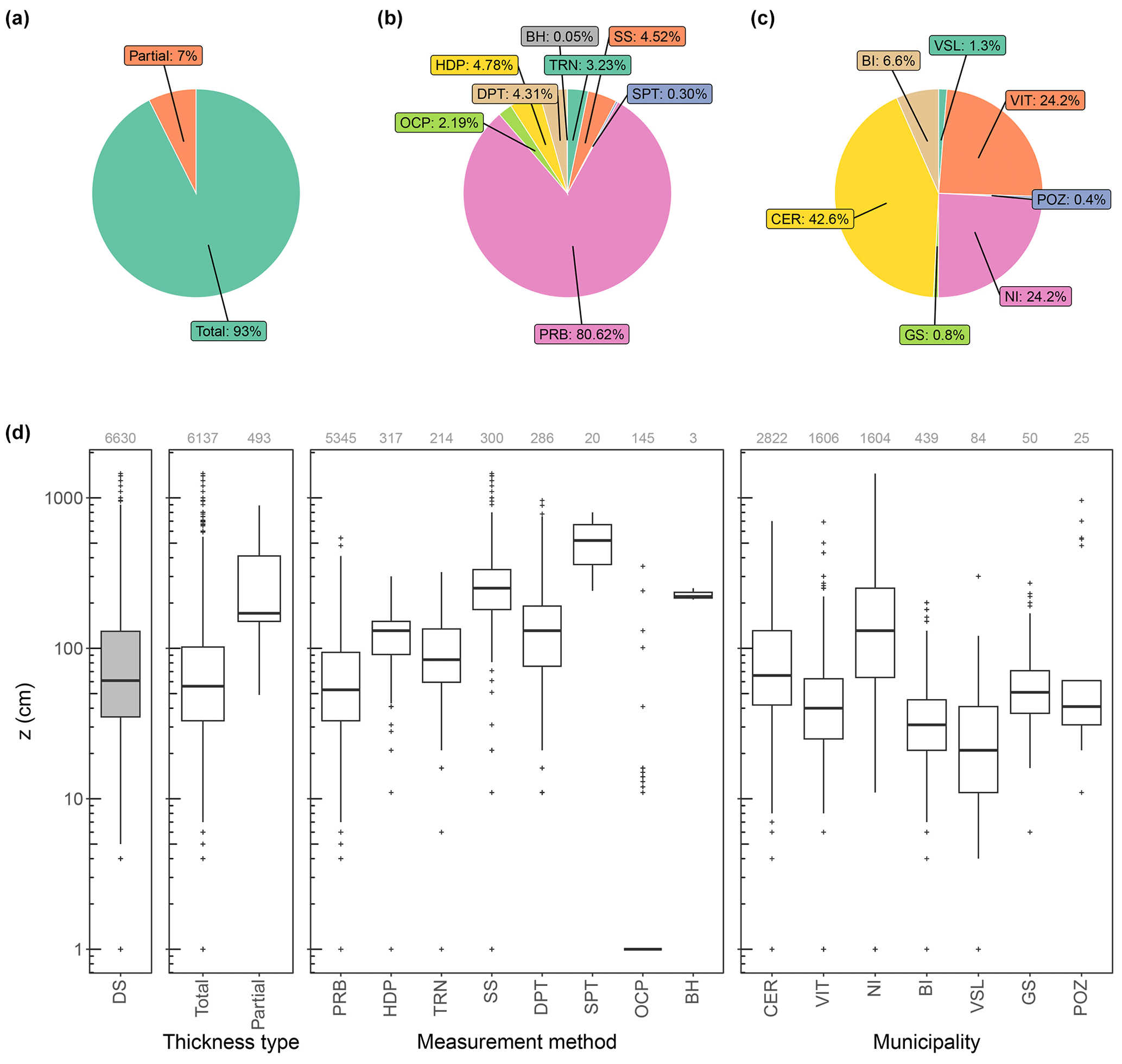
Figure 5 An overview of the field-based thickness measurements of the fallout pyroclastic deposit in study area: (a) proportion of total and partial measurements; (b) proportion of the measurements regarding the methodology; (c) proportion of the measurements in each municipality; and (d) variation of thickness considering the whole dataset, total and partial measurements, measurement methods, and municipalities. DS: the dataset, OCP: the outcrop, PRB: the probing test, TRN: the trench, HDP: the hand-dug pit, DPT: the dynamic cone penetration tests, BH: the borehole, SS: the seismic survey, SPT: the standard penetration test, NI: Nocera Inferiore, BI: Bagnoli Irpino, CER: Cervinara, VIT: Vitulano, GS: Gioia Sannitica, POZ: Pozzilli, and VSL: Villa Santa Lucia. It is noteworthy that the partial measurements are excluded before modeling thickness in this study.

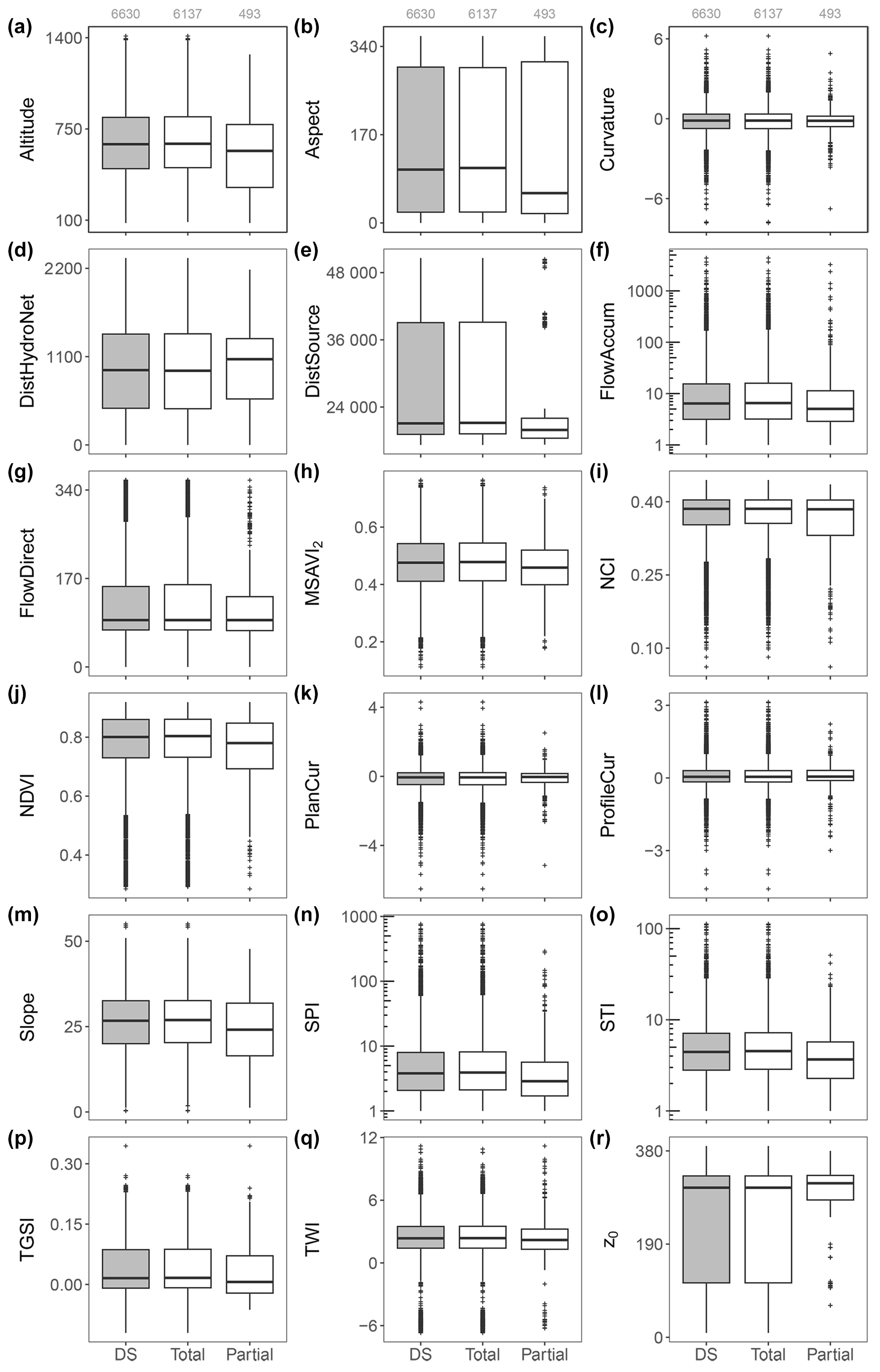
Figure 6 Range of the values for predictor variables referred to in the whole dataset (DS) and in the total and partial measurements. DistHydroNet: the distance to hydrographic network, DistSource: the distance to the source, FlowAccum: the flow accumulation, FlowDirect: the flow direction, PlanCur: the plan curvature, and ProfileCur: the profile curvature. It is noteworthy that the partial measurements are excluded before thickness modeling in this study.

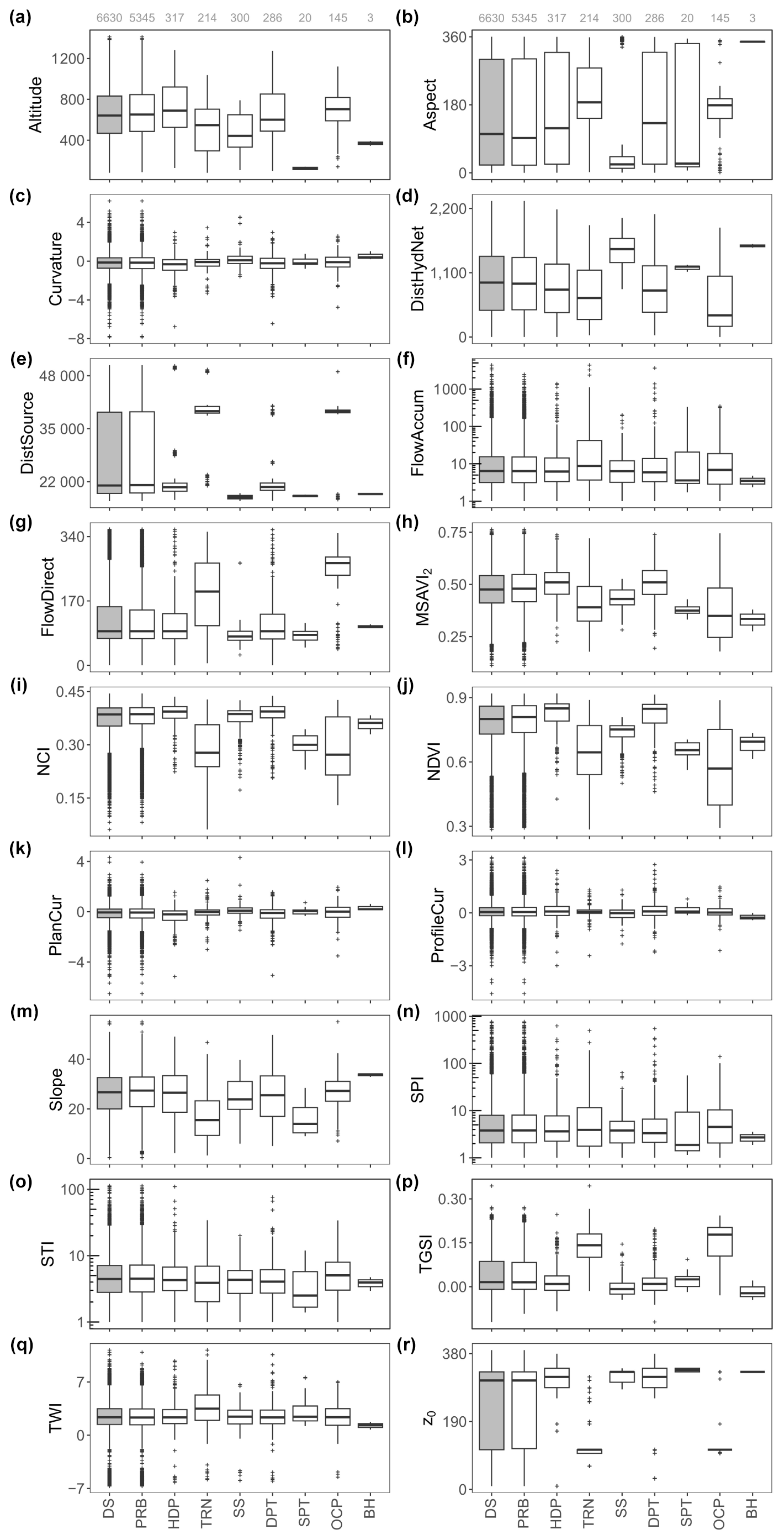
Figure 7 Range of values for the predictor variables referred to in the whole dataset (DS) and in the different measurement methods (from PRB to BH). See caption of Fig. 5 for the abbreviations. It is noteworthy that the partial measurements (n=493) are excluded before thickness modeling in this study.

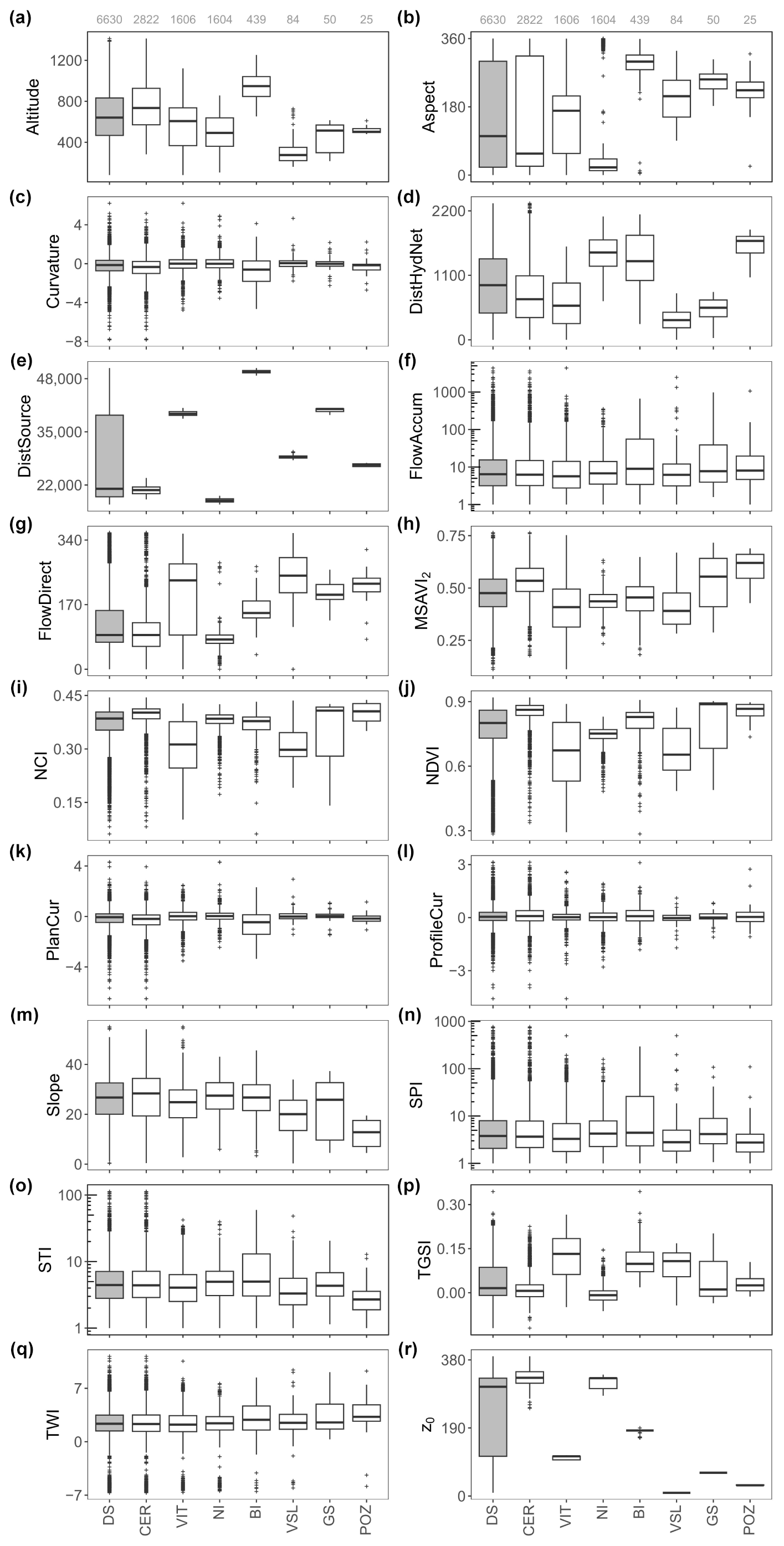
Figure 8 Range of values for the predictor variables referred to in the whole dataset (DS) and in the municipalities (from CER to POZ). See caption of Fig. 5 for the abbreviations. It is noteworthy that the partial measurements (n=493) are excluded before thickness modeling in this study.

The surveys were mainly conducted in the Cervinara, Nocera Inferiore, and Vitulano territories (43 %, 24 %, and 24 %, respectively; Fig. 5c). The median thickness values are above 60 cm in Nocera Inferiore and Cervinara, while they fluctuate around 35 cm in the other municipalities (Fig. 5d). The values of predictor variables assigned to the total and partial measurement points are almost similar, but the minor differences have some interesting interpretations (Fig. 6). Compared to the stations for total measurements, the median values in Fig. 6 show that thickness is partially recorded in the measurement points with lower altitudes, distances to the source, and slope degrees but higher distances to the hydrographic network (Fig. 6a, d, e, and m). In addition, the distance of these stations to the hydrographic network is greater than that of the total thickness measurement points (Fig. 6d). This last aspect confirms that the bedrock is usually not reached by investigation and that the thickness is therefore greater as one moves away from the hydrographic network, with the torrential erosive intensity being lower. The similarity between Fig. 5d (i.e., the three boxplots on the left) and Fig. 6r probably reveals that z₀ is a good indicator of z.

The measurement points are also categorized in terms of the measurement methods (Fig. 7) to underline the category-based variation of the predictor variables. The insignificant variation of the variables for the stations investigated using borehole stratigraphic data explains the few field-based observations under this category. Standard penetration tests and seismic surveys are the preferred methods in the low-altitude locations far from the hydrographic network and near the source (Fig. 7a, d, and e). On the contrary, the thickness of the fallout pyroclastic deposits is investigated via trenches and outcrops at the measurement points farthest from the source (Fig. 7e). The lowest computed z₀ values are related to these stations as well (Fig. 7r). Curvature, plan curvature, profile curvature, and topographic wetness index (TWI) show very similar distributions regardless of the methodology (Fig. 7c, k, l, and q). The ranges of the predictor values are compared for different municipalities (Fig. 8) to provide some spatial information on the variables. For instance, Bagnoli Irpino and Villa Santa Lucia occur at the highest and lowest altitudes, respectively (Fig. 8a). The latter has the lowest distance to the hydrographic network, along with the minimum calculated z₀ and measured z values (Figs. 8d, r, and 5d, respectively). Cervinara and Nocera Inferiore are the closest municipalities to the source (Fig. 8e), where the greatest z₀ values are calculated (Fig. 8r), above 65 % of the measurements are performed (Fig. 5c), and the highest z values are recorded (the right panel of Fig. 5d). Taking into account Figs. 1 and 8r, significantly higher fallout pyroclastic deposits were emplaced by volcanic activities in the eastern sector of the study area. The discussion in this section indicates a relatively high level of heterogeneity in the variables. The presence of many data outliers can also be visually verified in Figs. 5–8. These characteristics of the data suggest a complex relationship between the predictor variables and the thickness of fallout pyroclastic deposits, which can be better modeled by means of machine learning techniques rather than by the standard models employed in the literature.

5 The estimated thickness of fallout pyroclastic deposits: results

In this article, we proposed applying RF and STPW approaches that train a model on the training subset and make predictions on the test subset. The dataset of 6137 measurement points was, therefore, randomly divided into training (n=4294) and test (n=1843) subsets (Fig. 4), and the same subsets were used in all predictive models to evaluate the performance of the competing models. For the training data, the thickness is estimated by GPT, SAPT, SEPT, STPW, and RF models. The predictions for different models are then combined and the associated errors are investigated. Finally, the prediction errors are computed for both the training and test subsets, and the predictive accuracy tests are implemented for evaluating differences in estimations. This section explains the results in detail.

5.1 Training stepwise regression and random forest

The STPW model is used for selecting the best subset of variables in terms of explicative power for the pyroclastic thickness deposit. Given an initial set of 18 independent variables, only 8 relevant ones are chosen by the STPW model for making predictions (Table 3): distance to the hydrographic network, distance to the source, altitude, z₀, aspect, plan curvature, modified secondary soil-adjusted vegetation index (MSAVI₂), and normalized clay index (NCI) (for a detailed description of the variables, see Table 2). All these variables are very relevant in determining the thickness of fallout pyroclastic deposits as they control the erosion–deposition processes. The estimated parameters shown in Table 3 are then used for predicting the thickness values in the test subset.

Table 3 List of the variables selected by STPW model for making predictions in the training subset. The estimated parameters, standard errors, and p values are also reported.

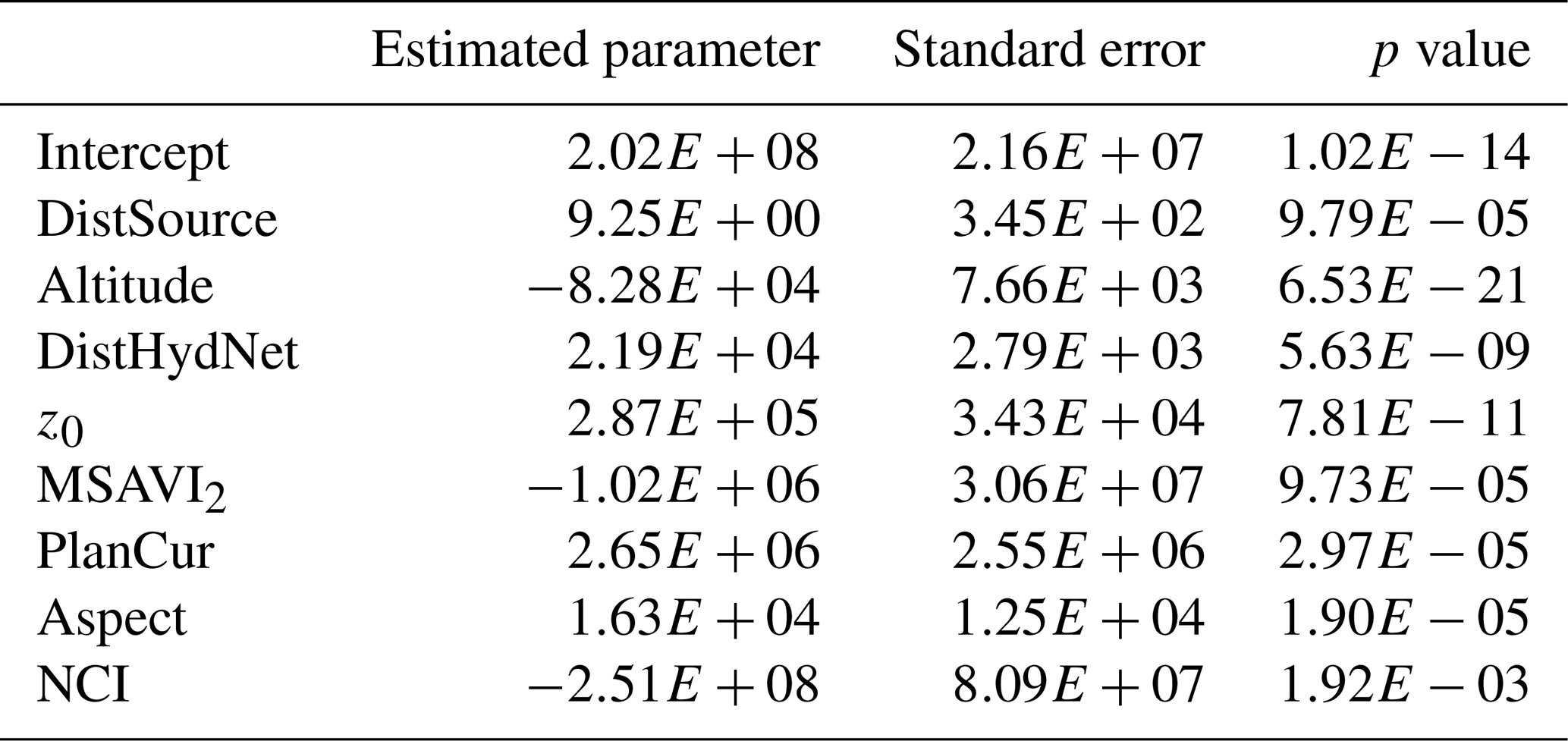
In order to train random forest model representatively, different values are assigned to m_try, min.node.size, replace, and sample.fraction, and a list of all possible combinations of the hyperparameters (882 in our case) is generated. The random forest is then trained for all combinations, and the optimum value for each hyperparameter (m_try=5, min.node.size = 17, replace = True, and sample.fraction = 0.632) is determined based on the model with the least error. The out-of-bag error is then investigated for different number of trees, and num.trees = 530 is determined for training a model with the least error (Fig. S1a). Figure S1b and c show that altitude, z₀, normalized difference vegetation index (NDVI), distance to the hydrographic network, NCI, and topsoil grain size index (TGSI) account for the most important variables in training the model based on both variable importance metrics (i.e., impurity and permutation). Compared to the STPW model, distance to the source is the only variable excluded before RF modeling to avoid unrealistic estimations.

5.2 Predicted thickness values

Table 4 shows the RMSE and MAE for all models applied to both the training and test subsets. The relevant differences in prediction accuracy are evident (e.g., RMSE = 184.52 and MAE = 157.10 for SAPT vs. RMSE = 79.11 and MAE = 46.44 for RF). Considering the single models applied to the training subset, both the STPW and RF models improve the predictive accuracy measures compared with GPT, SAPT, and SEPT. It is worth mentioning that the RF model (RMSE = 79.11 and MAE = 46.44) outperforms other approaches (RMSE >89 and MAE >55) for the training dataset. This suggests that the predictor variables discussed in Sect. 5.1 play a crucial role in estimating the thickness of fallout pyroclastic deposits.

Table 4 Prediction accuracy results. Best model in bold. GPT refers to geomorphological pyroclastic thickness, SAPT: slope angle pyroclastic thickness, SEPT: slope exponential pyroclastic thickness, STPW: stepwise regression, RF: random forest, SA: the simple average, MV: the minimum variance, OLS: ordinary least squares, and LAD: least absolute deviation.

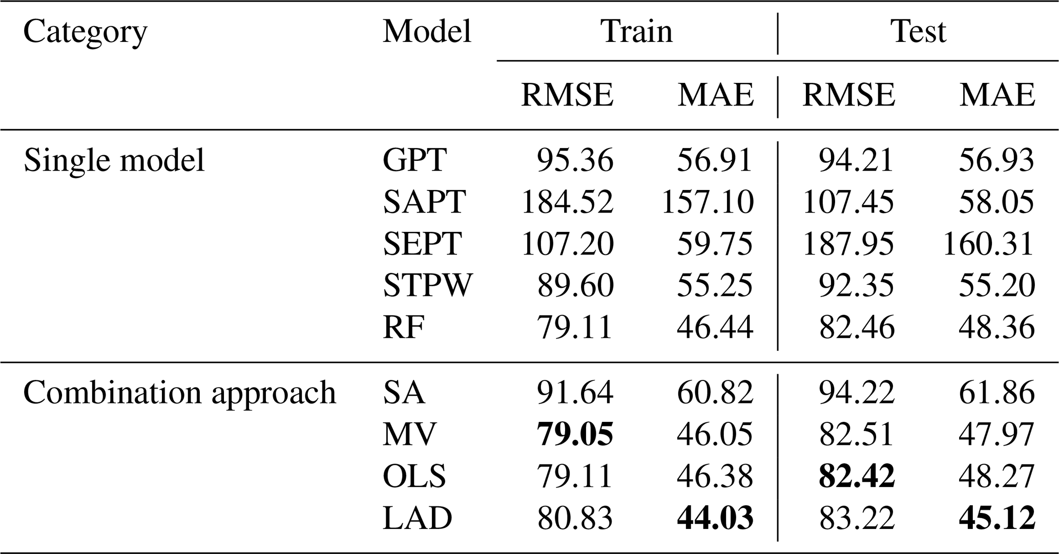
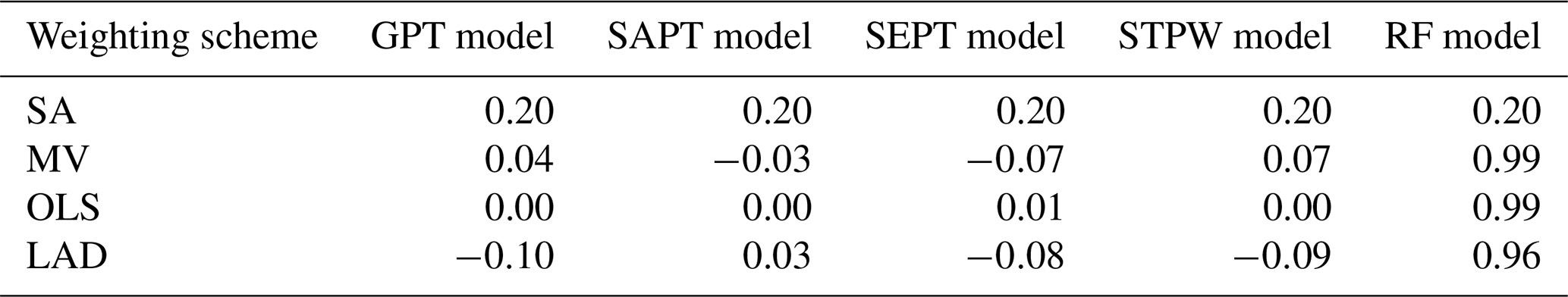
In the next step, the thickness predictions for the training subset (obtained from the single models) underwent a combination approach using the weighting schemes in Table 5. Except for the SA method that assigns equal weights to the models, all the weighting schemes assign the largest weight to RF, which is the most accurate one among the single models. The accuracy measures for the combination models are shown in the lower part of Table 4. According to the results for the training subset (Table 4), the RMSE shows that the predictions of the SA approach are the worst, while the MV approach provides better accuracy than the RF model. The MAE function indicates that the LAD method improves the accuracy by about 5 % compared to the RF model.

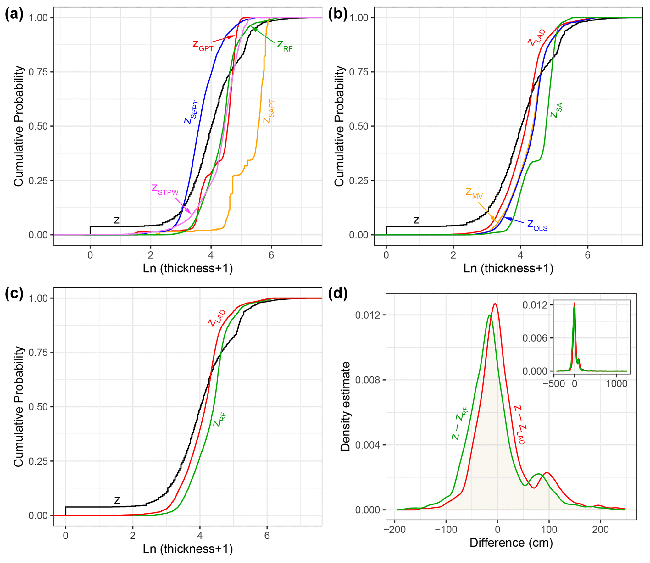
Figure 9 Cumulative probability of the field-based thickness measurements (z) against the estimations by single models and combination approaches (a and b, respectively). In panel (c), only z, the estimations by the best single model, and the estimations by the best combination approach are visualized. However, panel (d) represents the difference between z and the thickness estimated by the best single model and the thickness estimated by the best combination technique. In this figure, z represents thickness, but the subscript refers to the method of estimation. The estimations (n=6137) for both the training and test subsets are visualized. GPT: geomorphological pyroclastic thickness, SAPT: slope angle pyroclastic thickness, SEPT: slope exponential pyroclastic thickness, STPW: stepwise regression, RF: random forest, SA: simple average, MV: the minimum variance, OLS: ordinary least squares, and LAD: least absolute deviation.

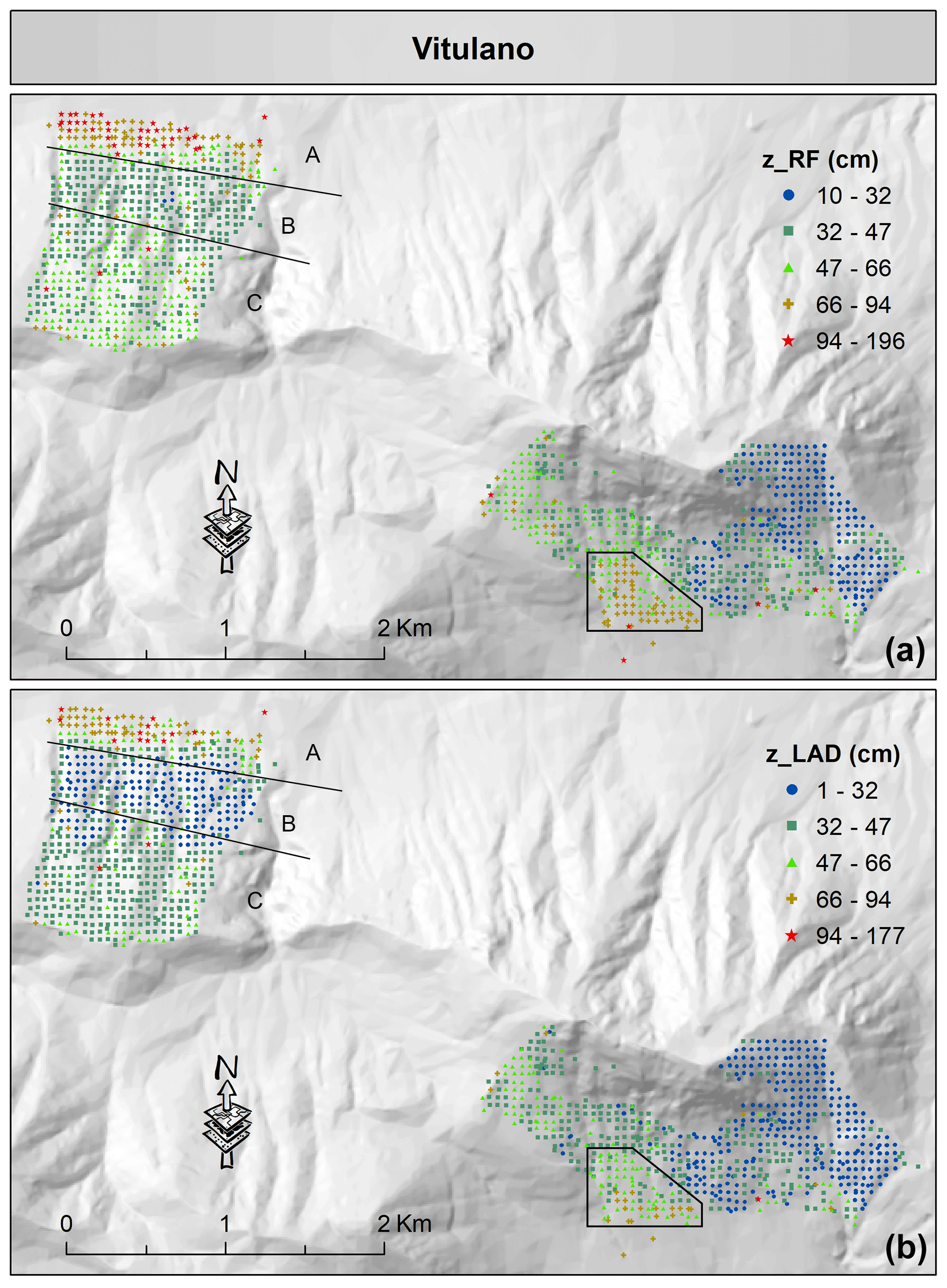
Figure 10 Spatial visualization of the predicted thickness of fallout pyroclastic deposits by the random forest as the best single model (a) and by LAD as the best combination approach (b) for the Vitulano municipality. It is worth mentioning that the random forest predictions are classified by the Jenks Natural Breaks algorithm, and the thresholds are implemented for generating the map of LAD predictions. Please see the text for more information about A, B, and C labels, together with the black box. Although symbols of different shapes and colors are used for the classes, the spatially dense measurement points do not allow an application of a larger symbol size. In the electronic version of this article, please zoom in on the figure to distinguish between different symbols based on the shape (if required).

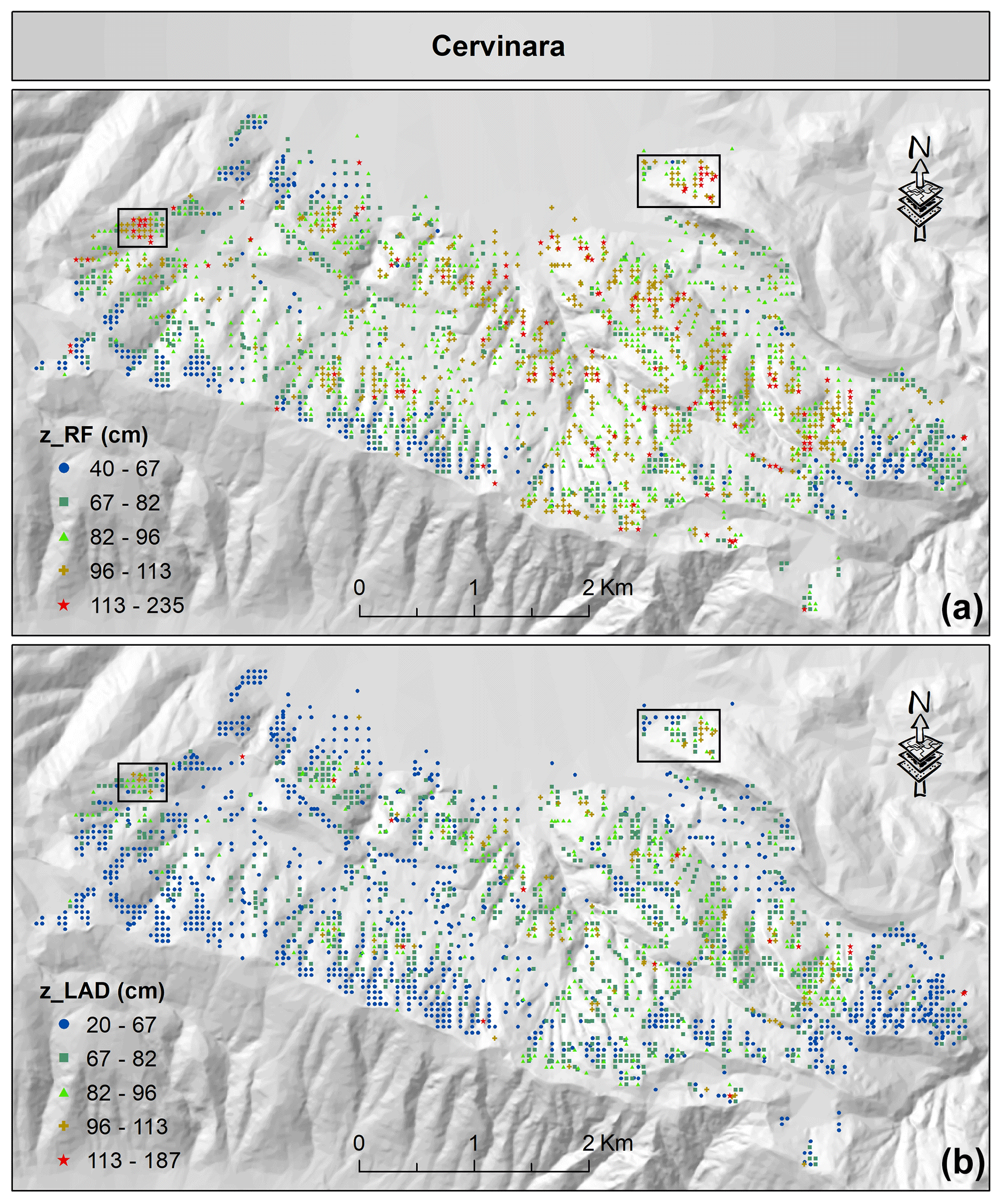
Figure 11 Spatial visualization of the predicted thickness of fallout pyroclastic deposits by the random forest as the best single model (a) and by LAD as the best combination approach (b) for the Cervinara municipality. It is worth mentioning that the random forest predictions are classified by the Jenks Natural Breaks algorithm, and the thresholds are implemented for generating the map of LAD predictions. Please see the text for more information about the black boxes. Although symbols of different shapes and colors are used for the classes, the spatially dense measurement points do not allow an application of a larger symbol size. In the electronic version of this article, please zoom in on the figure to distinguish between different symbols based on the shape (if required).

Table 5 The weights for making predictions in the training subset with combination approaches. The abbreviations are as defined in Fig. 3.

Then both single models and the alternative combination approaches for the test subset are compared in terms of RMSE and MAE (see the last two columns of Table 4). Among the single models, RF provides the most accurate results (RMSE = 82.46 and MAE = 55.20), but the combination of the RF predictions with those of the other models enhances the accuracy. In particular, the OLS approach reduces the RMSE to 82.42, and the LAD method lowers the MAE to 45.12. Regarding the lower sensitivity of the MAE to data outliers, the LAD combination could be considered to be the most representative model. The LAD combination improved the accuracy by 7.2 % compared to the RF model. The improvement is above 26 % respect to the GPT model, the best single model proposed in the previous studies.

Finally, pairwise EPA tests are applied to account for the uncertainty in the results and to investigate whether the differences in predictive performance are statistically significant in the test subset (Table 6).

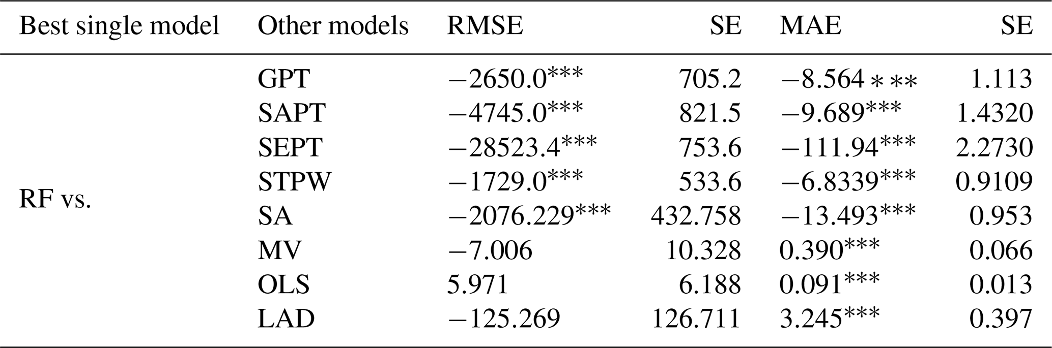
The upper part of Table 6 compares RF as the best single model with the other single models and reveals that the differences are statistically significant. In other words, the observed differences in the predictive performance of the models are not explained by the randomness of the data, and the RF model provides the most accurate thickness estimation. The negative RMSE and MAE values indicate that the RF model has a lower average prediction error than the other single models. On the other hand, the lower part of Table 6 shows the pairwise comparison of the RF model with all the combination approaches. A positive RMSE or MAE value suggests that the predictions of the combination approach are more accurate. In terms of squared error loss, the OLS combination approach provides the most accurate predictions compared to the RF model, but it is noteworthy that the RMSE and OLS are both sensitive to data outliers, as explained in Sect. 3.3. Regarding the MAE, statistically significant improvement is observed when combination approaches are applied (except for the SA method; p<0.01). The greatest statistically significant constant value of the LAD method demonstrates that this combination technique is suitable for predicting the thickness of fallout pyroclastic deposits in unmeasured locations. The results are in accordance with those in Table 4.

Table 6 Equal predictive accuracy tests, applied to the test subset (n=1843), for comparing the best single model (RF) with the other ones. Under the null hypothesis, the two models provide equal predictive accuracy. SE refers to the heteroskedasticity robust standard error. The abbreviations are as defined in Fig. 3. ${}^{***}$ indicates p value <0.01.

6 Discussion

In this section, the cumulative probabilities of the estimated thickness (for both the training and test subsets) obtained by various methods are compared in Fig. 9a and b. Regarding the single models (Fig. 9a), significant underestimation of the SEPT model and noticeable overestimation of the SAPT model are evident. These models have the highest RMSE and MAE values among the single models (Table 4). The distributions of the values obtained by the GPT, RF, and STPW models share more similarity with those of field-based measurements. Although the STPW model performs better than RF in predicting the smaller values, the RF model outperforms the single models, which agrees with Table 4. Taking Fig. 9b into account, all combination techniques work more effectively than the LAD approach in the upper 25 % of thickness values. The overall estimations of the LAD approach are, however, more consistent with the field-based measurements, being confirmed by the accuracy measures in Table 4.

The results of the RF model and the LAD approach are also visualized in Fig. 9c for the sake of comparison, representing that the values estimated by the former are greater than those of the latter. The LAD approach outperforms the RF model in a wide range of the field-based thickness values, and it is, therefore, the best model for predicting the thickness of fallout pyroclastic deposits in the study area. Figure 9d demonstrates that the LAD estimations are less biased.

The estimated thickness values of fallout pyroclastic deposits obtained by the RF model and the LAD combination approach in Vitulano, Cervinara, and Nocera Inferiore are visualized in Figs. 10–12 to investigate the differences between the spatial patterns. Although the spatial distribution remained generally unchanged, the legends of the maps reveal that the estimated thickness values obtained by the LAD combination approach decreased, as shown before (Fig. 9c). For instance, in Vitulano (Fig. 10), the estimations range from 10 to 196 cm in the RF model, which is reduced to 1–177 cm in the LAD combination approach. This is also evident in most estimations of the bottom-right box, in which the values are reduced from 66–94 cm to about 32–66 cm, or in the top-left corner of the map: A (47–196 cm) > C (32–66 cm) > B (32–47 cm) in the RF model vs. A (47–94 cm) > C (32–47 cm) > B (1–32 cm) in the LAD combination approach. The same decline could be observed in Cervinara and Nocera Inferiore as well. To facilitate a quick comparison, two boxes are drawn in Figs. 11 and 12 that highlight the sectors with a clear change. A few estimations exceed 113 cm in the lower panel of Fig. 11, which is contrary to the upper panel generated by the RF model in Cervinara.

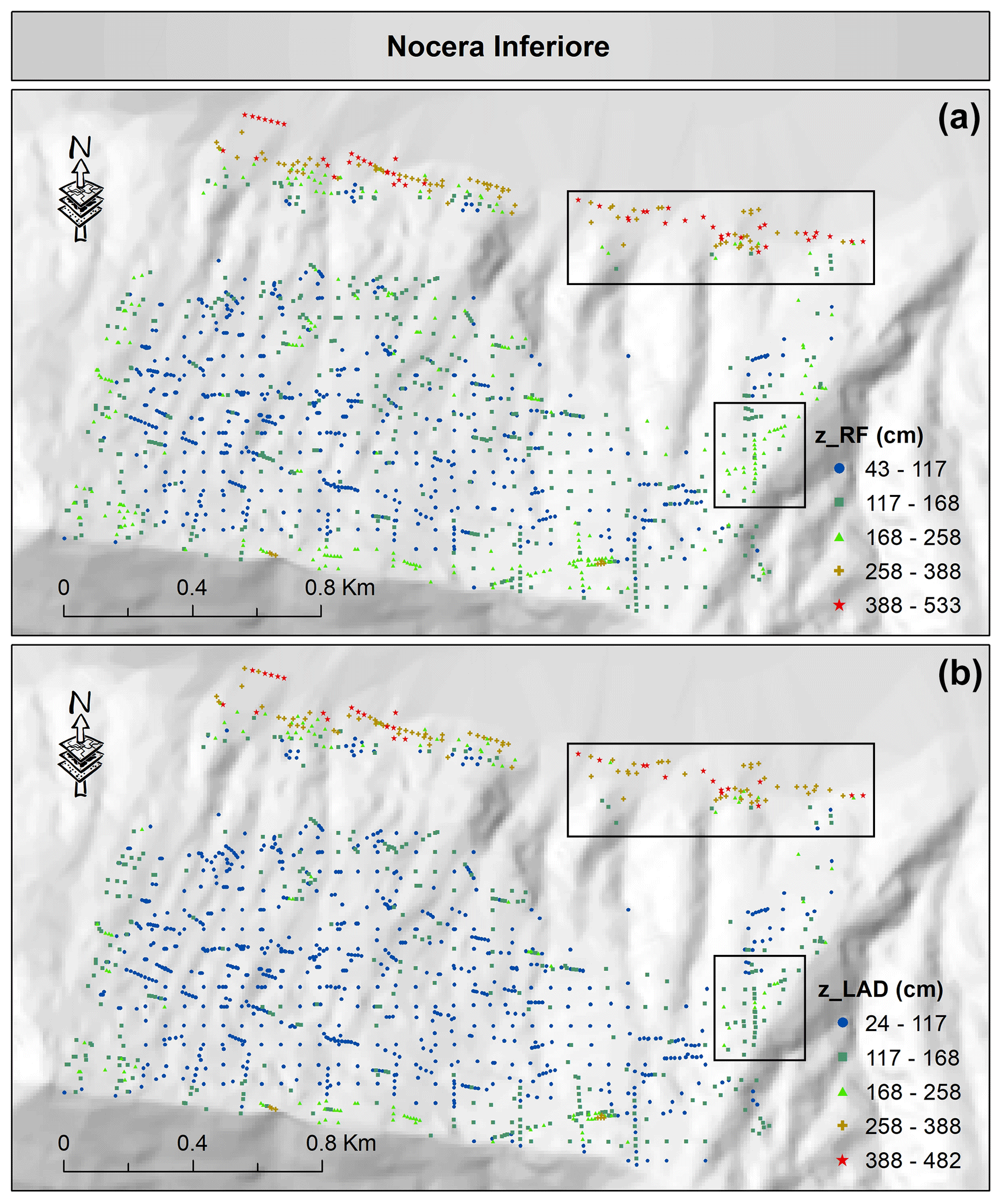
Figure 12 Spatial visualization of the predicted thickness of fallout pyroclastic deposits by the random forest as the best single model (a) and by the LAD as the best combination approach (b) for the Nocera Inferiore municipality. It is worth mentioning that the RF predictions are classified by the Jenks Natural Breaks algorithm, and the thresholds are implemented for generating the map of LAD predictions. Please see the text for more information about the black boxes. Although symbols of different shapes and colors are used for the classes, the spatially dense measurement points do not allow the application of a larger symbol size. In the electronic version of this article, please zoom in on the figure to distinguish between different symbols based on the shape (if required).

7 Data availability

The field-based thickness measurements of fallout pyroclastic deposits are accessible on Zenodo (Matano et al., 2023; https://doi.org/10.5281/zenodo.8399487).

8 Conclusion and future research direction

A given volcano might have several eruptive events. In an explosive volcanic eruption, the height of the ash plume and the wind characteristics mainly determine the ash dispersal pattern. However, the expected spatial thickness may be continuously altered by the soil-forming and denudation processes. It is, therefore, a daunting task to estimate thickness of fallout pyroclastic deposits that we observe today. The GPT, SAPT, and SEPT models were proposed in previous studies to address this issue, but this article tries to apply other models for the first time to estimate thickness more accurately around the Somma–Vesuvius, Phlegrean Fields, and Roccamonfina volcanoes in Campania, southern Italy.

First, we prepared a database of 6137 field-based thickness measurements with 18 predictor variables. Second, the STPW model and the RF machine learning technique were implemented for thickness modeling, and the results were compared with those of the GPT, SAPT, and SEPT models. The RF estimations (RMSE = 79.11 and MAE = 46.44 for the training subset and RMSE = 82.46 and MAE = 48.36 for the test subset) evidently outperformed the other models (RMSE >89.60 and MAE >55.25 for the training subset and RMSE = 92.35 and MAE >55.20 for the test subset). Third, the SA, LAD, MV, and OLS approaches were considered to combine the predictions of the five above-mentioned single models and to obtain more accurate thickness estimations. It was indicated that the LAD approach returns the best results in terms of MAE. Thus, the estimations with the RF and LAD methods (as a single model and a combination approach, respectively) were less biased in Campania. The thickness values obtained from the RF and LAD in Vitulano, Cervinara, and Nocera Inferiore were applied for spatial analysis, and it was demonstrated that the estimated values of the LAD approach are smaller than those of RF, but the spatial patterns do not change significantly. The results showed that following the methodology in this article and generating a map using the estimations of the LAD combination approach provides the most representative estimations in the study area.

In the future, we will consider a set of more representative predictor variables (if any) and collect a larger field-based thickness measurement dataset for estimating thickness in the unmeasured locations (i.e., out-of-sample predictions from a statistical point of view) more accurately. This would help in generating a regional map of the thickness of fallout pyroclastic deposits in Campania, which plays a key role in hydrogeological and volcanological studies and in managing geohazards in the areas covered with loose pyroclastic materials. Furthermore, we will aim to define the best statistical combinations at local levels by means of cluster-wise techniques.