the Creative Commons Attribution 4.0 License.
the Creative Commons Attribution 4.0 License.
 | 13 Sep 2024
The SDUST2022GRA global marine gravity anomalies recovered from radar and laser altimeter data: contribution of ICESat-2 laser altimetry
Zhen Li
Chengcheng Zhu
Xin Liu
Cheinway Hwang
Sergey Lebedev
Xiaotao Chang
Anatoly Soloviev
Heping Sun
The global marine gravity anomaly model is predominantly recovered from along-track radar altimeter data. Despite significant advances in gravity anomaly recovery, the improvement of the gravity anomaly model remains constrained by the absence of cross-track geoid gradients and the reduction in radar altimeter data, especially in coastal and high-latitude regions. ICESat-2 laser altimetry, with a three-pair laser beam configuration, a small footprint, and a near-polar orbit, facilitates the determination of cross-track geoid gradients and provides valid observations in certain regions. We present an ICESat-2 altimeter data processing strategy that includes the determination of cross-track geoid gradients and the combination of along-track and cross-track geoid gradients. Utilizing these methods, we developed a new global marine gravity model, SDUST2022GRA, from radar and laser altimeter data. Different weight determination methods were applied to each type of altimeter datum. The precision and spatial resolution of SDUST2022GRA were assessed against published altimeter-derived global gravity anomaly models (DTU17, V32.1, NSOAS22) and shipborne gravity measurements. SDUST2022GRA achieved a global precision of 4.43 mGal, representing an improvement of approximately 0.22 mGal over existing altimeter-derived models. In local coastal and high-latitude regions, SDUST2022GRA showed an enhancement of 0.16–0.24 mGal compared to the other models. The spatial resolution of SDUST2022GRA is approximately 20 km in certain regions, which is slightly superior to the other models. The percentage contribution of ICESat-2 to the improvement of the gravity anomaly model is 4.3 % in low- to mid-latitude regions by comparing SDUST2022GRA with ICESat-2 to SDUST2021GRA without ICESat-2, and this is increasing in coastal regions. These assessments suggest that SDUST2022GRA is a reliable global marine gravity anomaly model. The SDUST2022GRA data are freely available at https://doi.org/10.5281/zenodo.8337387 (Li et al., 2023).
- Article
(7145 KB) - Full-text XML
- BibTeX
- EndNote


Marine gravity is a critical piece of marine environmental information, and accurately recovering marine gravity anomalies is essential for marine geophysics, marine geology, and marine dynamics (Hwang and Chang, 2014; Sandwell et al., 2014; Bidel et al., 2018; Wang et al., 2020). Since the late 1970s, satellite altimetry has provided global sea surface height (SSH) observations, which are associated with the time-invariant marine geoid. Because of its global coverage and consistent accuracy, satellite altimetry is a vital technique for the recovery of marine gravity anomalies, complementing in situ gravity measurements (Andersen and Knudsen, 1998; Watts et al., 2020; Zhang et al., 2021).
The current method for gravity recovery from altimetry is well-established. Normally, the north–south component and east–west component of the deflection of the vertical (DOV) on a regular grid, derived from along-track geoid gradients (GGs), are used to recover the marine gravity anomaly model using the inverse Vening Meinesz formula or Laplace's equation (Sandwell and Smith, 1997; Hwang et al., 2002). The accumulation of altimeter data and advances in data processing methods have led to the publication and continual refinement of marine gravity anomaly models (Andersen et al., 2021; Zhu et al., 2020). However, there remains a need to improve the accuracy of the global marine gravity anomaly model for investigating small-scale undersea features and tectonics (Y. Yu et al., 2021; Sandwell et al., 2021).
The recovery of marine gravity anomalies primarily relies on along-track radar altimeter data (Hwang et al., 2006; Andersen et al., 2010; Wu et al., 2019). Due to the north–south inclination of the satellite orbit, the precision of the northern component of the altimeter-derived DOV model is generally higher than that of the eastern component (Che et al., 2021; Jin et al., 2022). The unbalanced accuracy of DOV components severely restricts the improvement of the gravity anomaly model (Hwang, 1998; Annan and Wan, 2021). New altimeter modes such as twin-satellite altimetry and wide-swath altimetry aim to provide cross-track altimeter data for addressing the unbalanced accuracy (Bao et al., 2013; D. Yu et al., 2021; Jin et al., 2022). Consequently, incorporating cross-track altimeter data is essential for enhancing the marine gravity anomaly model.
Radar altimeter data are crucial for recovering gravity anomalies, providing centimeter accuracy in SSH observations (Vignudelli et al., 2011). Conventional radar altimeter data have a large pulse-limited nadir footprint spanning a few kilometers in diameter (Escudier et al., 2018). Even with a synthetic aperture radar (SAR) altimeter using Doppler shift technology, the pulse-limited footprint is reduced to a few hundred meters only in the along-track direction (Egido and Smith, 2016; Vignudelli et al., 2019). The radar echo signal used for SSH observations is susceptible to interference from non-homogeneous reflective surfaces in coastal regions, degrading SSH accuracy and reducing the number of valid SSH observations (Hwang et al., 2006; Escudier et al., 2018). Although altimeter data processing, such as waveform retracking, contributes to improving the quality of SSHs, the precision of gravity anomalies recovered from degraded SSHs in coastal regions is still inferior to that in the open ocean (Passaro et al., 2018; Fernandes et al., 2021). Additionally, few altimetry missions provide altimeter data for regions with latitudes above 66° due to orbital inclination constraints (Li et al., 2022), resulting in degraded gravity anomaly model accuracy in high-latitude regions (Andersen and Knudsen, 2019; Ling et al., 2021). Therefore, incorporating altimeter data with new characteristics is crucial for improving the marine gravity anomaly model, especially in coastal and high-latitude regions.
The ICESat-2 laser altimetry mission (Markus et al., 2017), launched in September 2018, carries the Advanced Topographic Laser Altimeter System (ATLAS). ATLAS provides three pairs of laser beam altimeter data, with approximately 3.3 km spacing for each pair in the cross-track direction. This configuration allows for the determination of cross-track height slopes (Buzzanga et al., 2021). This provides an opportunity to mitigate the unbalanced accuracy of the DOV caused by only using along-track altimeter data. In addition, the ICESat-2 laser beam has a nominal 17 m diameter photon footprint, making SSH observations less susceptible to interference from non-homogeneous reflective surfaces compared to radar altimeter data. Although the small footprint might be adversely affected by surface ocean waves, it is particularly useful for SSH observations in coastal regions (Wang et al., 2022; Wang and Sneeuw, 2024). Furthermore, ICESat-2 provides near-global coverage with a 92° inclination, complementing radar altimeter data in high-latitude regions. SSH observations from ICESat-2 have been investigated for applications such as ocean topography recovery, DOV determination, and SSH anomaly variation examination, confirming them to be comparable to the best radar altimeter data (D. Yu et al., 2021; Che et al., 2021; Bagnardi et al., 2021). However, ICESat-2 altimeter data are rarely used in published global marine gravity anomaly models.
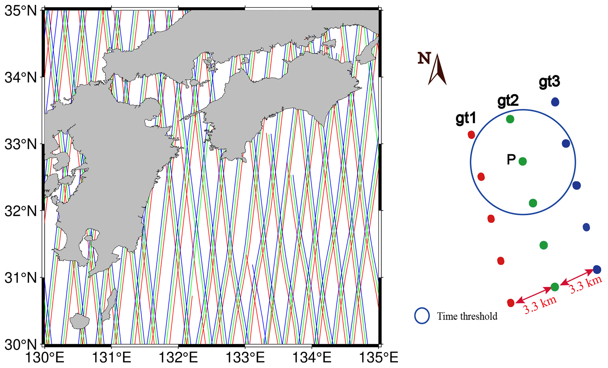
Figure 1ICESat-2 ground track of three strong beams (cycle_0011).
The unique characteristics of ICESat-2 laser altimeter data motivate us to develop a new global marine gravity anomaly model and investigate its potential for gravity anomaly recovery. First, we present the ICESat-2 altimeter data processing method for determining cross-track GGs and combining along-track and cross-track altimeter data. The new global marine gravity anomaly model, SDUST2022GRA, is recovered from multi-satellite altimeter data, including radar and laser altimeter data. Second, we assess the accuracy of SDUST2022GRA by comparing published global marine gravity models (NSOAS22, DTU17, and V32.1) and shipborne gravity measurements. Finally, we analyze the contribution of ICESat-2 laser altimeter data to the gravity anomaly recovery by comparing SDUST2022GRA and SDUS2021GRA without using ICESat-2 data.
2.1 ICESat-2 laser altimeter data
The ICESat-2 mission provides three pairs of laser beams, each pair consisting of a strong beam and a weak beam with an energy ratio of about 4:1, to measure Earth's surface elevations, e.g., land or sea ice elevation, land or water vegetation elevation, and ocean elevation. For ocean elevation observations, ICESat-2 typically only downlinks strong beam data due to the low surface reflectance. The ICESat-2 product, ocean elevation ATL 12 (level 3, version 5), provides along-track SSHs from three strong beams and is available from NASA's Earth Science Data Systems (EarthData, https://search.earthdata.nasa.gov/, last access: 6 June 2024).
In ATL12, the SSHs have been corrected for atmospheric delay, dynamic atmospheric errors, tidal errors, sea state bias, and other factors (Morison et al., 2021). The ocean tide correction is derived from the global ocean tide model GOT4.8 with a resolution of 0.5° (Ray, 2012). However, the recent global ocean tide model FES2014 (Carrere et al., 2015), with a resolution of 0.125°, is used for the Level2+ (L2P) product of radar altimeter data. Therefore, the correction from FES2014 instead of GOT4.8 is used for the SSH from ICESat-2, which is consistent with the product of the radar altimeter data. The SSH is referenced to the WGS84 reference ellipsoid (ITRF2014 reference framework; Morison et al., 2021). The ICESat-2 ground track of three strong beams from one cycle (91 d) is shown in Fig. 1. Because of the laser observation dependent on the weather conditions, the along-track ground distance of SSH observations is variable, between 70 m and 7 km.
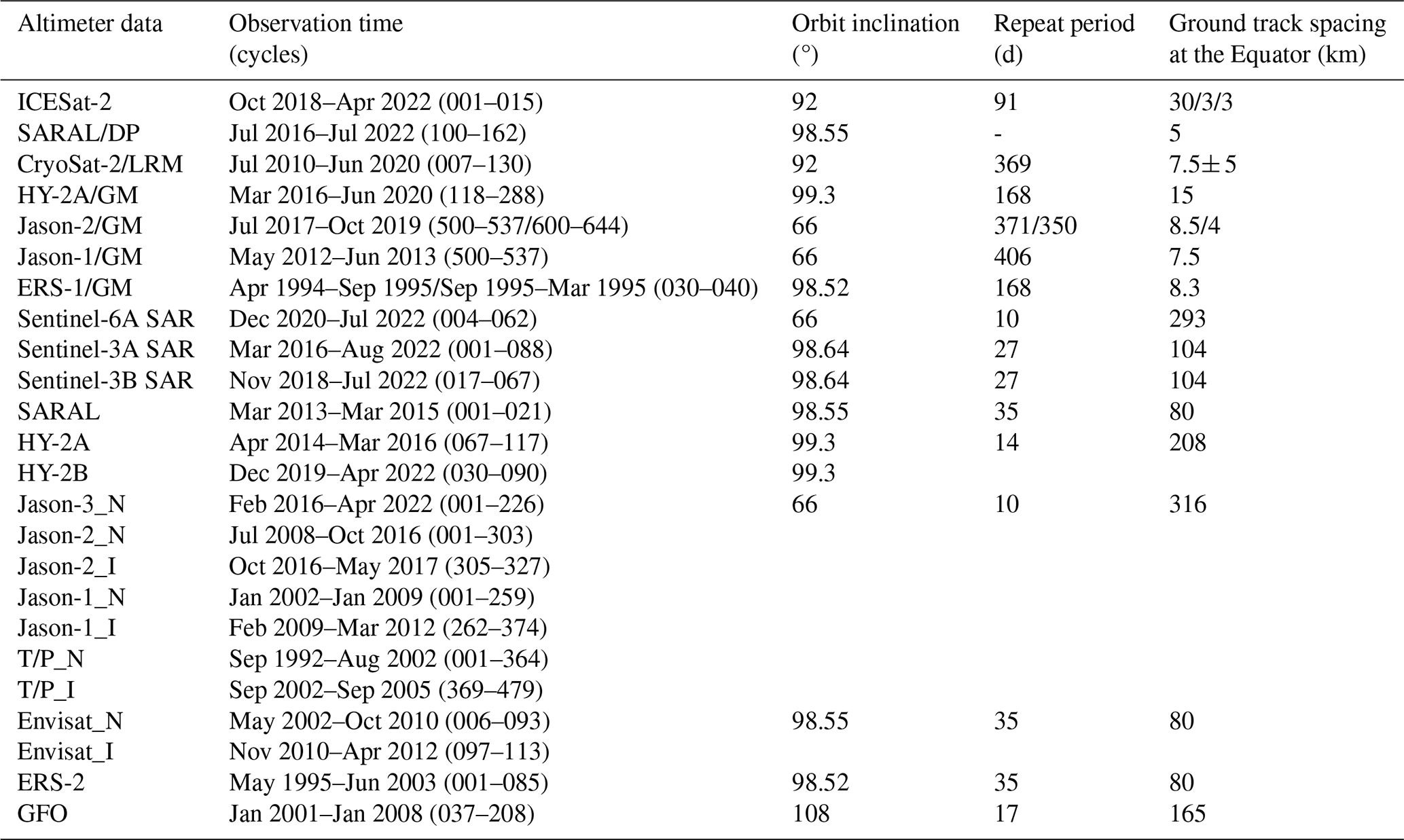
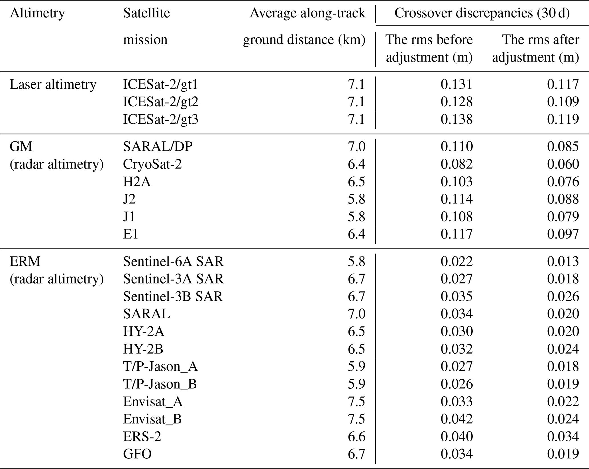
Table 1Altimeter data information for global marine field recovery.
2.2 Multi-satellite radar altimeter data
The multi-satellite radar altimeter data used in SDUST2022GRA are similar to those from the previously published SDUST2021GRA (Zhu et al., 2022), which are primarily from altimetry missions after the 1990s. Although the ERS-1 altimeter data make little contribution to the improvement of the gravity model, the geodetic mission (GM) altimeter data are used for the addition of data coverage, especially in high-latitude regions. In addition, the SAR altimeter data from new missions (Sentinel-3A/3B, Sentinel-6A) are also used in SDUST2022GRA. The information about the used altimeter data is presented in Table 1. The nominal tracks and interleaved tracks from exact repeat missions (ERMs) are labeled “_N” and “_I”, respectively.
All SSHs of radar altimeter data were obtained from the non-time-critical L2P (version 3) product, which formed the reprocessing Geophysical Data Records (GDR), except for Sentinel-6A. L2P is available at AVISO (https://www.aviso.altimetry.fr/, last access: 1 July 2024). The Sentinel-6 SAR altimeter data are from the high-resolution non-time-critical ocean surface topography product, which is available from NASA's EarthData (https://search.earthdata.nasa.gov/, last access: 6 June 2024). All SSHs are from Ku-band altimeter data, except for the SSH of SARAL, which is from Ka-band altimeter data. The SSHs from radar altimeter data are both at a 1 Hz sampling frequency and are referenced to the WGS84 ellipsoid (CNES, 2024).
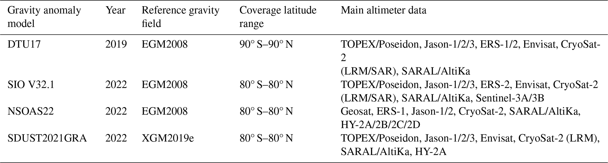
2.3 Global marine gravity anomaly models
Earth's gravitational field is typically used as the reference field in the recovery of gravity anomalies using the remove–restore technique. The recently published XGM2019e is a global gravity model that combines the satellite gravity model GOCO06s, the marine gravity anomaly model DTU13, and gravity measurements over land and ocean (Zingerle et al., 2020). Gravity anomalies on a 1′ × 1′ grid from XGM2019e up to degree and order 2190 are available from the International Centre for Global Earth Models (ICGEM, http://icgem.gfz-potsdam.de/calcgrid, last access: 9 September 2024); these are used as the reference gravity field for the recovery of SDUST2022GRA.
The recently published global marine gravity anomaly models were obtained to assess the performance of SDUST2022GRA. The commonly recognized global marine gravity anomaly models are the Sandwell and Smith (S&S) series from the Scripps Institution of Oceanography (SIO) and the DTU series from the Technical University of Denmark. The publicly available models include V32.1 of the S&S series (Sandwell et al., 2021) and DTU17 of the DTU series. Additionally, other gravity models were obtained, e.g., NSOAS22 (Zhang et al., 2022) recovered from incorporating HY-2 altimeter data and SDUST2021GRA (Zhu et al., 2022) recovered using the improved data fusion method. It is important to note that these models do not yet utilize ICESat-2 laser altimeter data. Table 2 lists the information on the global marine gravity anomaly models. According to several studies, the root mean square (rms) of the difference between altimeter-derived gravity anomaly models and shipborne gravity anomalies is approximately 3–5 mGal (Yu et al., 2022; Wan et al., 2022).
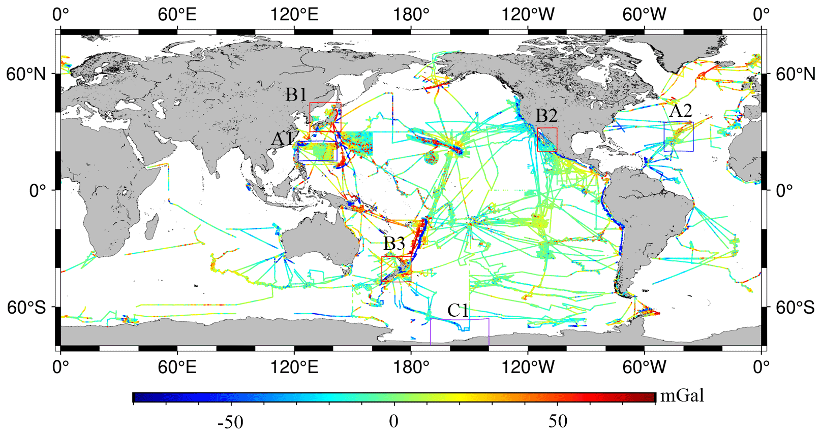
Figure 2Global available shipborne gravity anomalies from the NCEI after the 1990s and the local study regions.
2.4 Shipborne gravity anomaly measurements
Shipborne gravity, as with in situ gravity measurements, is also used to assess the accuracy of the gravity anomaly model recovered from altimetry. In general, shipborne gravity anomalies have higher accuracy and spatial resolution along ship routes compared to the altimeter-derived gravity anomaly model. Global shipborne gravity anomalies after the 1990s were obtained from the U.S. National Centers for Environmental Information (NCEI), taking into account the impact of ship navigation on the accuracy of gravity measurements. Gross errors in the shipborne gravity data were removed. First, gravity measurement cruises with significant errors were discarded, and outliers exceeding 3 times the standard deviation for each cruise were removed by comparison with XGM2019e. Second, system biases in gravity anomalies from each cruise, caused by gravimeter drift, were corrected using a quadratic polynomial (Hwang and Parsons, 1995). After data editing, the remaining shipborne gravity anomalies are 7 012 812 points (486 cruises) with a rejection rate of 2.9 %. The distribution of shipborne gravity anomalies is illustrated in Fig. 2.
Since global shipborne gravity anomalies are gathered from various agencies, the NCEI does not give information on the precision of shipborne gravity measurements. The precision of shipborne gravity is verified by the discrepancies of gravity anomalies at crossover points. In the global ocean, the total number of crossover points is 49 277, and the rms of discrepancies is about 3.99 mGal. The precision of shipborne gravity, about 2.82 mGal, is derived by dividing the rms by the square root of 2 based on the error propagation law. This is generally consistent with the shipborne gravimeter measurements of 1–3 mGal in magnitude (Zaki et al., 2022).
We selected six study regions characterized by SSH variations due to current or undersea features to investigate the recovery of gravity anomalies. These regions include two open-ocean regions (A1 and A2), three coastal regions (B1, B2, and B3), and a high-latitude region (C1), as illustrated in Fig. 2. Regions A1 and B1 are located in the Kuroshio region, and Region A2 is located in the North Atlantic near the Mid-Atlantic Ridge. Regions B2 and B3 are situated in the Gulf of California and the coastal regions of New Zealand, respectively. Region C1 is a part of the Southern Ocean, located in the eastern Ross Sea and influenced by the Antarctic Circumpolar Current.
3.1 Multi-satellite radar altimeter data processing
This is a conventional method for the recovery of gravity anomalies from along-track radar altimeter data. First, several errors in SSH observations are corrected, including instrument errors, atmosphere delays, and geophysical corrections. For ERM radar altimeter data, a simplified collinear adjustment is used to remove the residual time-variable error (Rapp et al., 1994; Yuan et al., 2023). For GM along-track altimeter data, Gaussian filtering is applied to remove the high-frequency error (Zhu et al., 2020). Second, the residual geoid heights are determined by removing the mean dynamic topography model and the reference geoid model from the corrected SSHs. The removed valve of MDT_CNES_CLS18 (Mulet et al., 2021) or the geoid model at the corresponding positions of SSHs is derived by the bivariate spline interpolation. The residual along-track GG is derived by
where eα,res is the residual GG with its azimuth (α) at the central location of points pt1 and pt2, and ΔNpt1 and ΔNpt2 are the residual geoid heights at pt1 and pt2, respectively. dpt1_pt2 is the spherical distance between the two points.
The residual GGs can be converted to the northern and eastern components of the DOV by using the least-squares collocation (LSC). The LSC is also a method of multi-satellite altimeter data fusion that determines the error variance from each altimeter datum. The error variance of the GG from each altimeter datum can be derived using the error propagation law of Eq. (1) while ignoring the distance error of two points as
where me is the standard deviation (SD) of GGs to determine the error variance (Cnn in the LSC) of GGs, and mssh,P and mssh,Q are the SDs of SSH observations at pt1 and pt2, respectively.
The crossover discrepancies of SSH and the iterative method are applied to determine the GG errors from Ku-band and Ka-band altimeter data, respectively. In the crossover adjustment, a residual SSH error is established using a combination function of a general polynomial and a trigonometric polynomial (Huang et al., 2008) as
where f(t) is the SSH correction, t is the observation time, and t0 and t1 are the beginning and end observation times of each ground track. ω is the angular frequency (), and a0, a1, Ci, and Si are unknown parameters to be solved by the least-squares method. The integer n is determined based on the number of crossover points.
The iterative method (Zhu et al., 2020) is applied for determining the error of GGs from the Ka-band altimeter data (SARAL/DP) and contributes to improving the accuracy of the marine gravity anomaly model. This method depends on the relationship between the error of altimeter-derived gravity, the error of GGs, and the average number of GGs as
where is the error variance of altimeter-derived gravity and ρ is the average number of GGs on a 1′ × 1′ grid. The unknown parameters β0 and β1 can be solved by the least-squares method based on the error variance of altimeter-derived gravity, the error of GGs, and the average number from each Ku-band altimeter datum.
The iterative equation for the error variance solution of GGs is
The initial value is determined using the gravity anomalies recovered from the initial errors of GGs (SARAL/DP) derived from the rms values of crossover discrepancies. The termination condition of the iteration is that the difference between the adjacent errors of GGs ( and ) is less than a threshold (provided in Sect. 4.2).
3.2 ICESat-2 laser altimeter data processing
The ICESat-2 SSH observations at varying length scales are resampled at 1 Hz for each beam to achieve a uniform distribution of SSHs. In the resampling, SSHs at varying length scales are fitted using a quadratic polynomial at latitude to mitigate the effect of high-frequency noise and outliers. Each 1 s SSH is used to solve polynomial coefficients and then produce SSHs at the median of the latitude. If the number of observations is less than the minimum required for solving polynomial coefficients, the 1 s SSHs are averaged directly to 1 Hz. The quadratic polynomial function of latitude is (Yu and Hwang, 2022)
where li is the SSH observation at point i within a time threshold, vi is the residual at point i, an φi is the latitude at point i. a, b, and c are the coefficients of the quadratic polynomial.
The method of determining cross-track GGs is presented using ICESat-2 multiple-beam observations. A major difference between the radar altimeter data and ICESat-2 laser altimeter data processing is the determination of cross-track GGs. In Eq. (1) of the last section, the along-track GG is determined from adjacent SSH observations on a single beam. To determine the cross-track GGs, it is necessary to select the associated SSHs from different beam observations. Otherwise, a cross-track GG with an azimuth that deviates from the east–west direction may not be able to mitigate the unbalanced accuracy of the DOV.
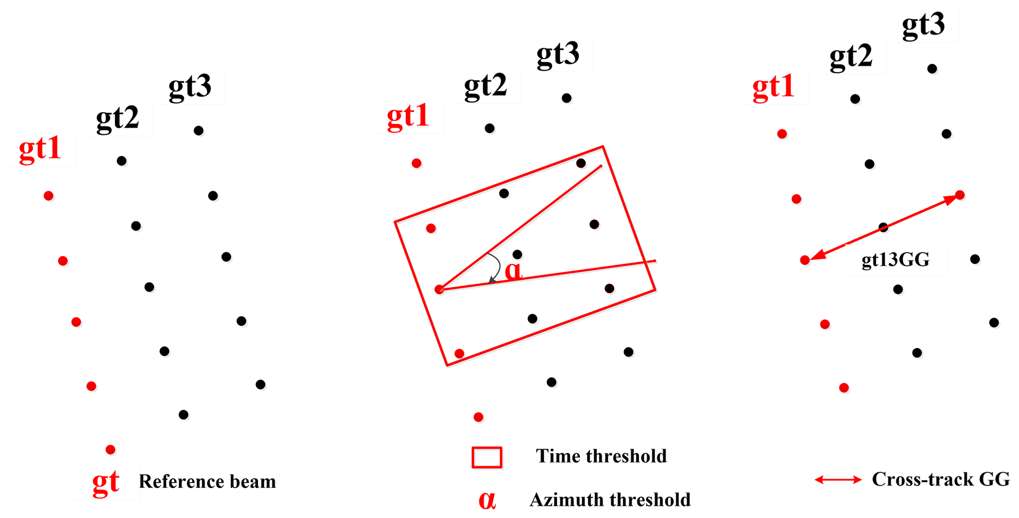
Figure 3The schematic diagram for determining the cross-track geoid gradients from the gt1 and gt3 beams of ICESat-2.
Since the three beams of ICESat-2 observations are not exactly simultaneous, the determination of cross-track GGs involves the following steps. (1) Select the beam with the maximum number of two-beam altimeter data as the reference altimeter data. (2) Based on the reference beam observations, determine the cross-track GGs within a time and azimuth threshold. (3) If there are multiple GGs for each reference observation, use only the cross-track GG with its azimuth closest to perpendicular to the orbit inclination for the recovery of gravity anomalies. A schematic diagram for determining the cross-track gt13 GGs from ICESat-2 altimeter data is shown in Fig. 3. The cross-track GG determination strategy is defined as follows:
where Numgt1, Numgt2, and Numgt3 are the numbers of each beam observation. Tref is the observation time of the reference beam, Ti is the observation time of the other beam, and αGG,i is the azimuth of the GG derived from two-beam observations at the number i. αref_inc is a reference azimuth perpendicular to the orbit inclination. T_Threshold is a time threshold, 1 s is selected as the time threshold to reduce the effect of random errors, A_Threshold is an azimuth threshold, and serves as an azimuth threshold to obtain GGs with their azimuth in the east–west direction.
Any two of the three tracks from ICESat-2 can be used to determine the cross-track GGs, named gt12, gt23, and gt13, respectively. The LSC is employed to fuse along-track and cross-track GGs based on their error variance. The error variance of cross-track GGs is derived from the errors of the associated SSHs.
Table 3The quality of the ICESat-2 SSHs and gravity models recovered from SSHs at varying length scales and resampled at 1 Hz.
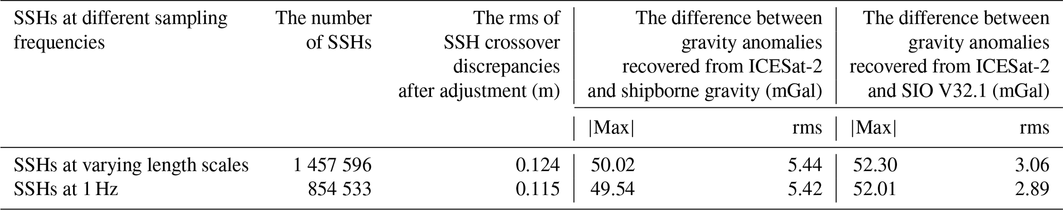
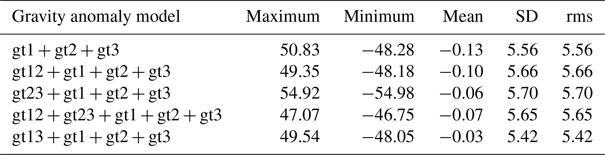
Table 4Differences between ICESat-2 altimeter-derived gravity and shipborne gravity (mGal).
3.3 Gravity anomaly recovery method
We determined the DOV components by the LSC (Hwang and Parsons, 1995; Hwang et al., 1998) as
where ξ and η are the residual northern and eastern components of the DOV. (or ) is the covariance matrix for the northern (or eastern) component of the DOV and GG, and Cee is the covariance matrix for the GGs. The diagonal matrix Cnn is the error variance of the GGs. eres,α is the residual GG.
The covariance function of residual disturbing potentials at the given distance can be calculated by errors of coefficients in the potential set with Model 4 proposed by Tscherning and Rapp (1974). Because the longitudinal and transverse components are isotropic, the covariance of longitudinal Cll and transverse Cmm for GGs can be derived using the covariance function. Therefore, the covariance matrices (, , and Cee) are obtained by (Hwang and Parsons, 1995)
where αeP and αeQ are azimuths of the satellite ground tracks at points P and Q, respectively. αPQ (or αQP) is the azimuth from P to Q (or from Q to P).
The gravity anomaly model is recovered by the inverse Vening Meinesz formula as (Hwang, 1998)
where γ0 is the normal gravity. is a kernel function of the spherical distance between two points. is the areal element of the unit sphere σ.
The gravity anomalies in the innermost zone are derived by
where ξy and ηx are obtained by numerical differentiations of the GGs. is the radius of the innermost zone. Δx and Δy are the grid intervals.
4.1 Gravity anomalies recovered from ICESat-2
For the recovery of gravity anomalies from ICESat-2 altimeter data, SSHs at varying length scales from ICESat-2 are resampled to 1 Hz to integrate them with radar altimeter data. The quality of SSHs and the recovered gravity anomalies from SSHs at different sampling frequencies are listed in Table 3. After resampling, the total number of SSHs is reduced, but the rms of SSH crossover discrepancies improves by about 0.01 m. Moreover, the rms of gravity anomalies from SSH at 1 Hz assessed by SIO V32.1 is slightly better than that of SSHs at varying length scales, which were assessed by shipborne gravity and SIO V32.1. Consequently, SSHs of ICESat-2 resampled at 1 Hz are used to recover global marine gravity anomalies.
The filtering radius is determined by the accuracy of the recovered gravity anomalies. For resampled SSHs of ICESat-2, the average ground distance of along-track adjacent observations is about 7 km, so the filtering radius with a multiple of 7 km is applied to recover marine gravity anomalies from along-track altimeter data. When the filtering radius is 7 km, the rms of the difference between gravity anomalies recovered from along-track altimeter data and shipborne gravity anomalies is 5.56 mGal. The result is better than that without using Gaussian filtering (5.61 mGal) or with a filtering radius of 14 km (5.58 mGal). Thus, the filtering radius of 7 km is selected for the recovery of gravity anomalies from ICESat-2 along-track SSHs.
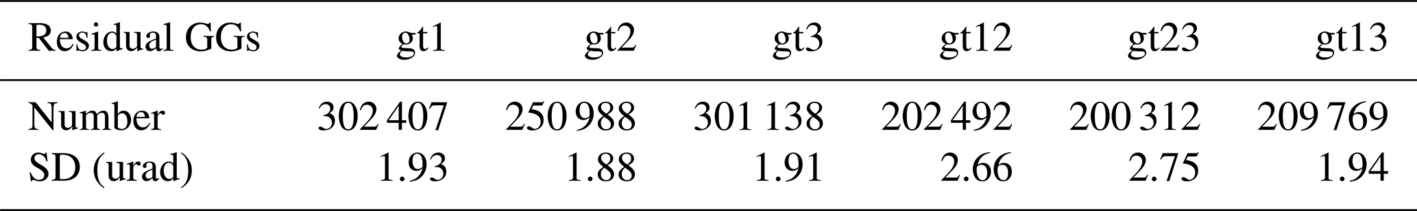
The combination of along-track and various cross-track GGs was investigated for the recovery of gravity anomalies. Specifically, combinations such as gt1 + gt2 + gt3 + gt12, gt1 + gt2 + gt3 + gt23, gt1 + gt2 + gt3 + gt13, and gt1 + gt2 + gt3 + gt12 + gt23 were analyzed. Table 4 lists the differences between gravity anomalies recovered from ICESat-2 and shipborne gravity. The rms of the gravity model recovered from gt1 + gt2 + gt3 + gt13 is 0.14 mGal better than that recovered from gt1 + gt2 + gt3, indicating that incorporating gt13 cross-track GGs improves the accuracy of the gravity anomaly model. However, incorporating gt12 or gt23 cross-track did not significantly enhance the model's accuracy. For this reason, we analyzed the number of observations from three beams for the precision of SSHs and GGs. Table 5 shows the quality (number and standard deviation) of along-track and cross-track GGs, while Table 6 lists the precision of SSHs from three beams. Although the precision of SSHs from the gt2 beam observation is slightly superior to that from gt1 or gt3, it is not straightforward to determine the precision of cross-track GGs. The precision of GG depends not only on the precision of SSHs, but also on the distance between the two points. The SD of gt13 GGs is closer to that of along-track GGs than those of gt12 and gt23. Furthermore, the number of gt2 beam observations is less than those of gt1 or gt3 beam observations, resulting in the number of gt13 cross-track GGs being higher than for the other cases. Therefore, the combination of along-track and gt13 cross-track GGs was used to recover marine gravity anomalies.
4.2 Global gravity anomalies recovered from all the altimeter data
The GG error from each altimeter datum is determined using SSH crossover discrepancies to fuse multi-satellite altimeter data, excluding SDRAL/DP altimeter data. Crossover discrepancies are determined based on the time interval between ascending and descending track observations. These discrepancies are computed from SSH observations collected within the smallest subcycle (approximately 30 d) of each altimetry mission, accounting for the number of crossover points and sea surface variations. For each ERM altimeter datum, the crossover discrepancies are obtained from SSHs after collinear adjustment without the limit of time. The rms of the SSH crossover discrepancies is detailed in Table 6.
Table 7Altimeter gravity error, geoid height error, and average number of geoid heights from Ku-band altimeter data.
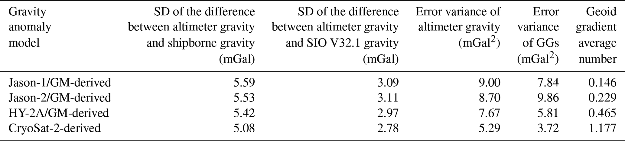
Table 8Marine gravity anomaly recovered from Ka-band altimeter data by different errors of geoid gradients.
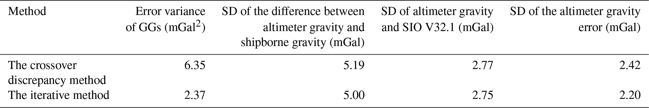
The GG error of SARAL/DP altimeter data is determined using the iterative method. Unknown parameters (β0 and β1) in the iterative equation (Eq. 5) are solved through a least-squares approach, considering the gravity anomaly model error, the GG error, and the average number within a 1′ × 1′ grid from each Ku-band GM altimeter datum, as shown in Table 7. Specifically, parameter β0 is found to be 8.96 and β1 to be −11.84 (R2 = 0.98, rms = 0.04). The GG errors determined by crossover discrepancies and the iterative method are shown in Table 8. Based on the GG error of SARAL/DP determined using the iterative method, the accuracy of gravity anomalies recovered from SARAL/DP shows an improvement of 9.1 % compared to the result of crossover discrepancies. Therefore, the GG error variance of 2.37 is used for SARAL/DP altimeter data.
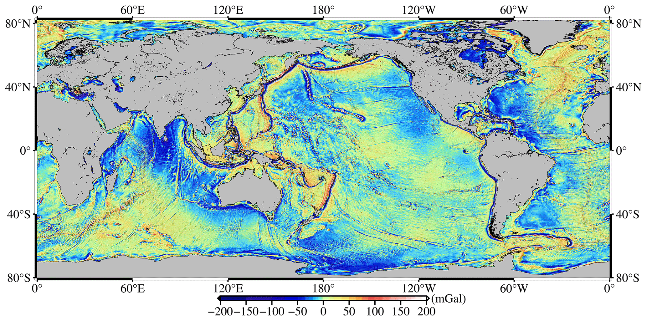
Figure 4The global marine gravity anomaly model SDUST2022GRA (free air) recovered from radar and laser altimeter data.
The accuracy and execution time of gravity anomaly recovery are impacted by the window length of the LSC, which is connected to the amount of altimeter data. When the window length is 0.2°, the recovery of gravity anomalies is balanced between accuracy and execution time, as shown in Table 9. The global ocean region (80° S–82° N, 0–360° E) is divided into 144 (18 × 8, longitude by latitude) subregions for the recovery of the global marine gravity anomaly model, and each subregion is extended outward by 1° to mitigate the boundary differences in gravity anomalies. The new global marine gravity anomaly model SDUST2022GRA (free air) on a 1′ × 1′ grid is recovered from multi-satellite altimeter data, as shown in Fig. 4.
Table 9The accuracy and execution time of gravity anomalies recovered using different window lengths in a subregion (21° × 21°).
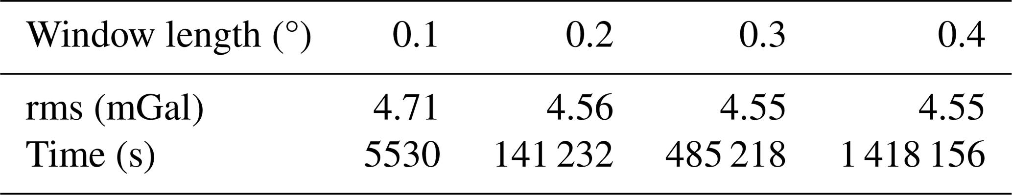
Time was calculated based on CPU AMD Ryzen 5-3500X 6-Core @ 3.60 GHz.
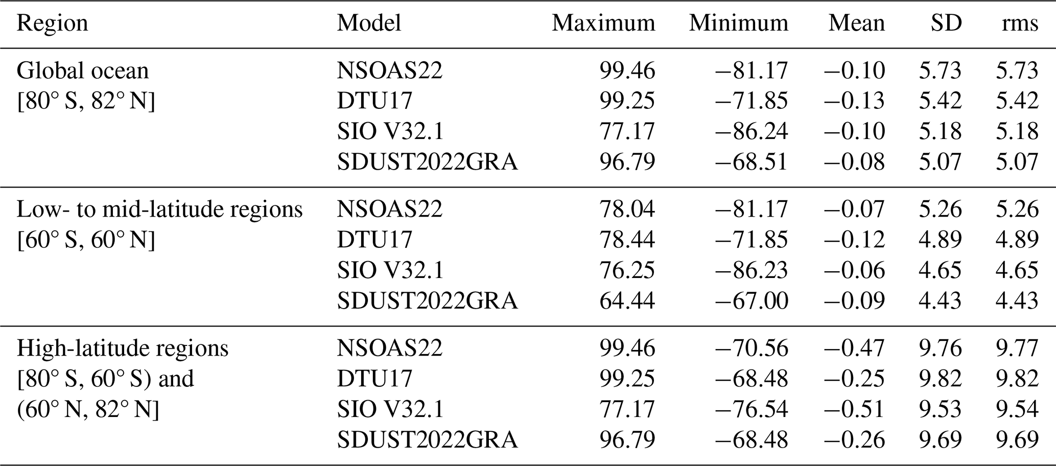
Table 10The difference between gravity anomaly models and global shipborne gravity (mGal).
4.3 Assessment of gravity anomaly model accuracy
The accuracy of SDUST2022GRA is evaluated using shipborne gravity anomalies in both global and local ocean regions. The differences between global gravity anomaly models and global shipborne gravity anomalies are listed in Table 10. Among the four global gravity anomaly models, the precision of SDUST2022GRA and SIO V32.1 is generally better than that of NSOAS22 and DTU17, which primarily benefitted from the addition of new altimeter data. In low- to mid-latitude regions, the precision of SDUST2022GRA is 4.43 mGal, representing an improvement of 0.22 mGal over SIO V32.1. Additionally, the precision of all gravity anomaly models in low- to mid-latitude regions is significantly better than that in high-latitude regions. The main reason for the degraded accuracy of gravity models in high-latitude regions is the reduction in altimeter data (see Fig. 8).
Table 11Mean and rms values of differences between gravity anomaly models and shipborne gravity in local regions (mGal).
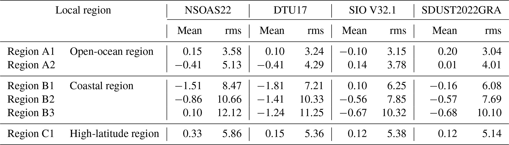
The precision of gravity anomaly models is further analyzed across different local regions, including open-ocean regions (A1 and A2), local coastal regions (B1, B2, and B3), and a high-latitude region (C1). The mean and rms differences between the gravity anomaly models and shipborne gravity anomalies in these regions are presented in Table 11. Notably, shipborne gravity models within 20 km of the coastline are used to assess the gravity anomaly model in coastal regions.
The precision of all gravity models in open-ocean regions is significantly better than that of gravity models in coastal and high-latitude regions. This shows that degraded SSH can significantly reduce the precision of gravity anomalies, especially in coastal regions and high-latitude regions. In local open-ocean regions, SIO V32.1 and SDUST2022GRA each have their own advantages resulting from unique improvement methods and the addition of altimeter data. For instance, SIO V32.1 benefits from the improvement of along-track SSH gradients derived from two-pass waveform retracking, while SDUST2022GRA gains from the fusion of along-track and cross-track GGs from multi-satellite altimeter data. In local coastal and high-latitude regions, the rms of SDUST2022GRA is 0.16–0.24 mGal better than that of SIO V32.1, which primarily benefitted from the valid observations from the ICESat-2 laser beam. This assessment suggests that SDUST2022GRA achieves a higher accuracy than other models in coastal regions. Thus, SDUST2022GRA recovered by incorporating ICESat-2 laser altimeter data is a reliable global marine gravity anomaly model.
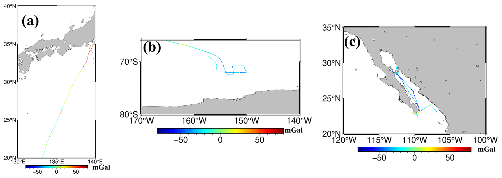
Figure 5Shipborne gravity (used to determine the CMS) of different cruises: (a) jare33l1 with an average distance interval of 0.45 km, (b) ew9201 with an average distance interval of 0.80 km, and (c) moce05mv with an average distance interval of 0.22 km.
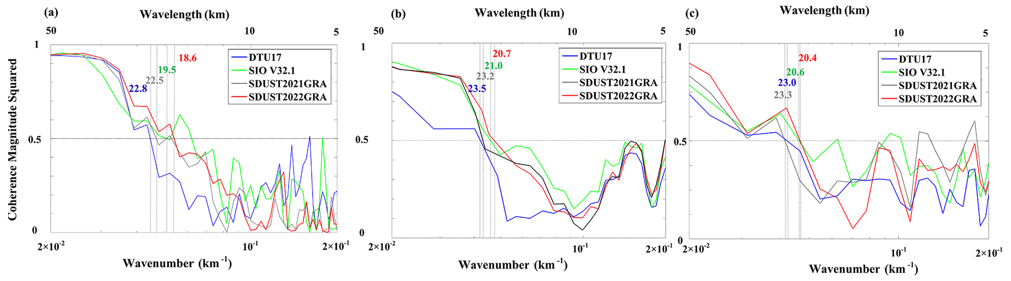
Figure 6The CMS between the gravity model and shipborne gravity of different cruises: (a) jare33l1, (b) ew9201, and (c) moce05mv.
4.4 Assessment of gravity anomaly model resolution
The spatial resolution of the gravity anomaly model in a local region is generally determined by spectral coherence analysis along shipborne gravity measurement tracks (Marks and Smith, 2016). The wavelength corresponding to a coherence-magnitude-squared (CMS) value of 0.5 is considered the highest spatial resolution of a gravity anomaly model. We used shipborne gravity anomalies from three cruises to determine the spatial resolutions of SDUST2022GRA, SIO V32.1, and DTU17, as shown in Fig. 5. The CMS value between the gravity anomaly models and shipborne gravity is presented in Fig. 6.
The wavelengths corresponding to a CMS value of 0.5 for SDUST2022GRA are 18.6 km in a local open-ocean region, 20.7 km in a high-latitude region, and 20.4 km in a coastal region, respectively. The spatial resolution of SDUST2022GRA in the open ocean is generally superior to that in high-latitude and coastal regions, which is largely related to the density of the altimeter data. The average number of altimeter data within a 1′ × 1′ grid in the open ocean are significantly higher than in high-latitude and coastal regions (see Fig. 8). The spatial resolution of SDUST2022GRA is approximately 20 km in a certain region, which is slightly better than that of DTU17 and SIO V32.1. Although SDUST2022GRA incorporates ICESat-2 altimeter data, the resolution is not significantly increased compared to DTU17 and SIO V32.1. Therefore, it is still a challenge to achieve a gravity anomaly model with a spatial resolution of a few kilometers from current altimeter data and with anticipation for the future wide-swath altimeter data from the Surface Water Ocean Topography (SWOT) altimetry mission (launch on 16 December 2022).
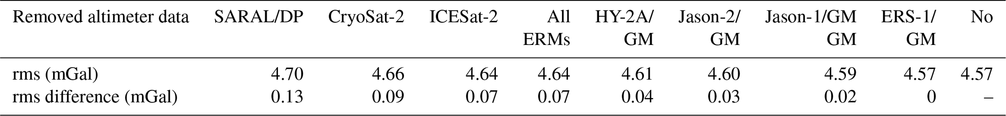
Table 12Ranking of the altimeter data contribution to the gravity anomaly model recovery.
4.5 Assessment of the ICESat-2 contribution
4.6 Contribution to model accuracy
The contribution of ICESat-2 to the improvement of the gravity anomaly model is investigated for precision and spatial resolution. It is widely recognized that GM radar altimeter data play an important role in the recovery of marine gravity anomalies. The role of ICESat-2 in the ranking of GM altimeter data is also determined according to the gravity anomaly model recovered by removing each GM altimeter datum from all altimeter data in the local region (20–40° N, 120–140° E). The rms differences between each gravity anomaly model and the shipborne gravity anomalies are listed in Table 12. The results demonstrate that the SARAL/DP and CryoSat-2 altimeter data provide a major improvement in the accuracy of the gravity anomaly model. Notably, the contribution of ICESat-2 to the improvement outperforms that of other GM altimeter data. This indicates that ICESat-2 altimeter data are on par with most GM altimeter data and form an extremely important dataset for improving marine gravity anomaly models. Additionally, all ERM data are essential for enhancing the global marine gravity anomaly model.
The contribution of ICESat-2 to the improvement in the accuracy of gravity anomalies is determined by comparing SDUST2022GRA, which incorporates ICESat-2, with SDUST2021GRA, which does not. Although the ICESat-2 altimeter data are not utilized in DTU17 or SIO V32.1, the differences between SDUST2022GRA and SIO V32.1 (or DTU17) also reflect variations caused by the different methods. Given that the SAR altimeter data from S3A/3B and S6A with sparse coverage are included in SDUST2022GRA, we initially determine the improvement in the precision of the gravity anomaly model. The rms difference between the gravity anomaly model only incorporating SAR altimeter data and shipborne gravity anomalies is 4.64 mGal, consistent with the rms of SDUST2021GRA without SAR altimeter data. This indicates that SAR altimeter data contribute minimally to the improvement of the gravity anomaly model. Therefore, the difference between SDUST2022GRA and SDUST2021GRA can be attributed primarily to the addition of ICESat-2 altimeter data.
Table 13The percentage contribution of ICESat-2 altimeter data in the global ocean region.
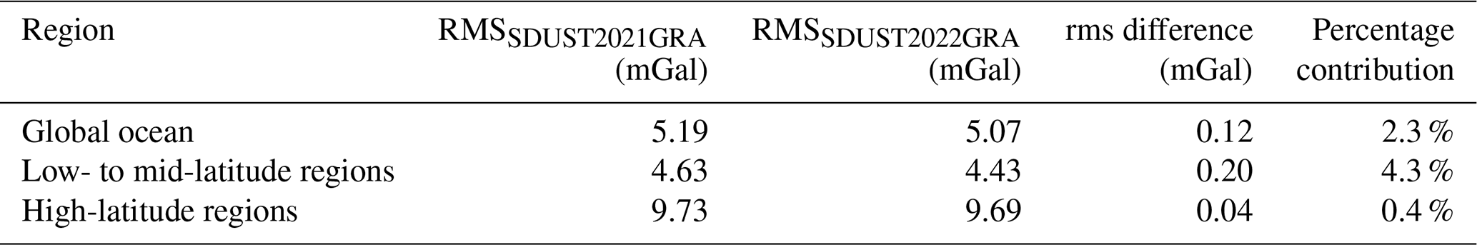
The percentage contribution of ICESat-2 to the improvement of the gravity anomaly model is defined as , representing the ratio of the improvement of the gravity model recovered by incorporating ICESat-2 into the improvement of the gravity model recovered from all altimeter data, as shown in Table 13. The percentage contribution of ICESat-2 is approximately 2.3 % in global ocean regions, while the number of SSHs from ICESat-2 makes up 10 % of all radar altimeter data. The percentage contribution is 4.3 % in low- to mid-latitude regions, indicating that the ICESat-2 altimeter data contribute to the improvement of the gravity anomaly model recovered from current radar altimeter data.
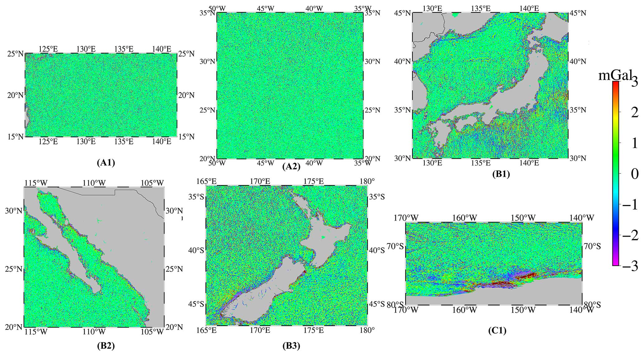
Figure 7The differences between SDUST2022GRA and SDUST2021GRA in different local regions.
The percentage contribution of ICESat-2 is also determined in various local regions, including the open-ocean, coastal, and high-latitude regions. The difference between SDUST2022GRA and SDUST2021GRA is shown in Fig. 7. The rms differences between both models are 0.83 and 0.72 mGal in the local open-ocean regions A1 and A2, respectively. In the coastal regions, note that the rms values are only derived from the difference within 20 km of the coastline. They are 1.29, 0.98, and 1.26 mGal in the local coastal regions B1, B2, and B3, respectively. The rms is 1.22 mGal in the local high-latitude region C1. These results indicate that the variation in the precision of the gravity model is visible by incorporating ICESat-2 altimeter data, especially in coastal and high-latitude regions.
Table 14The percentage contributions of ICESat-2 altimeter data in different local regions.
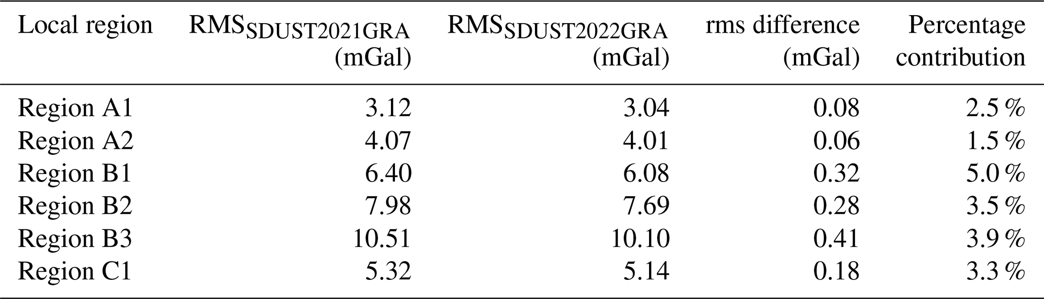
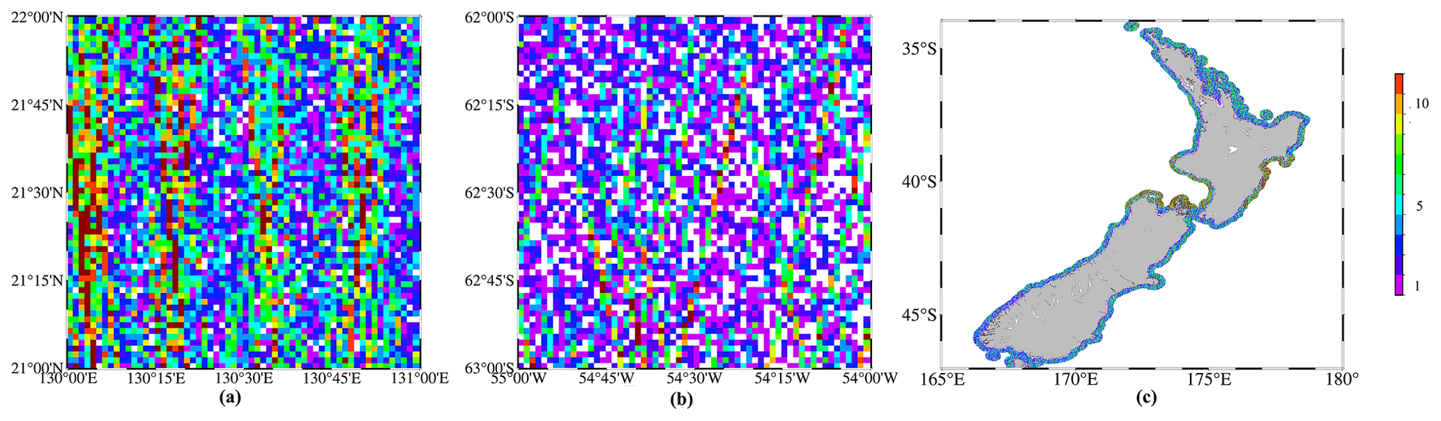
Figure 8The number of SSHs within the 1′ × 1′ grid in different local regions. (a) Open ocean with an average number of 3.5. (b) The high-latitude region with an average number of 2.1. (c) Coastal region with an average number of 1.9.
The percentage contribution of ICESat-2 in local coastal and high-latitude regions is generally higher than that in open-ocean regions, as shown in Table 14. To investigate the reason for this variation, the average number of GGs from all altimeter data within a 1′ × 1′ grid are calculated, as presented in Fig. 8. The average number of all radar altimeter data are relatively low in high-latitude and coastal regions, increasing by 50 % and 58 %, respectively. In open-ocean regions, however, this only increased by 21 %, which is lower than in high-latitude and coastal regions. This suggests that the high percentage contribution of ICESat-2 to the improvement is correlated with the increased proportion of the altimeter. In addition, 42 % and 35 % of the ICESat-2 altimeter data are located in a 1′ × 1′ grid where no radar altimeter data are available in high-latitude and coastal regions. In contrast, only 9 % of the ICESat-2 is located in a 1′ × 1′ grid in the open-ocean region. This indicates that ICESat-2 altimeter data provide complementary SSH coverage due to the reduction in radar altimeter data in high-latitude and coastal regions.
4.7 Contribution to model resolution
To analyze the contribution of ICESat-2 to the spatial resolution of the gravity anomaly model, we also compared the spatial resolution of SDUST2022GRA and SDUST2021GRA, as shown in Fig. 6. The wavelength corresponding to the CMS of 0.5 is reduced from 22.5 to 18.6 km in the local open ocean, from 23.2 to 20.7 km in the local high-latitude region, and from 23.3 to 20.4 km in the local coastal regions, respectively. The spatial resolution of the gravity anomaly model is slightly increased by incorporating ICESat-2 in a certain local region. However, the increased signal of the gravity anomaly is mainly from the power at wavelengths greater than 18 km. This suggests that the SSHs of ICESat-2 can improve the marine gravity anomaly model at wavelengths >18 km, but the contribution to higher resolution should be small.
The global marine gravity anomaly model, SDUST2022GRA, is available in the ZENODO repository at https://doi.org/10.5281/zenodo.8337387 (Li et al., 2023). The dataset includes global marine free-air gravity anomalies (WGS84 ellipsoid) in NetCDF file format (i.e., vector of latitudes, vector of longitudes, and matrix of gravity anomalies).
The recovery of the global marine gravity anomaly model primarily relies on along-track radar altimeter data. The advanced ICESat-2 laser altimetry mission, which provides SSHs from multiple beams and valid observations in high-latitude and coastal regions, offers the potential to mitigate unbalanced accuracy caused by traditional along-track altimeter data and to increase altimeter data availability for these challenging regions. A novel method for recovering gravity anomalies from cross-track altimeter data is proposed and utilized with ICESat-2 observations. The new global marine gravity model, SDUST2022GRA, is recovered from a combination of along-track and cross-track GGs from multi-satellite altimeter data. According to the recovered SDUST2022GRA and the previously published SDUST2021GRA without ICESat-2, we investigate the contribution of ICESat-2 to the recovery of the global marine gravity anomaly model, including the combination of along-track and cross-track altimeter data, as well as the addition of SSHs in high-latitude and coastal regions.
The precision of SDUST2022GRA is assessed using global shipborne gravity anomalies and published global marine gravity anomaly models (NSOAS22, DTU17, and SIO V32.1). The precision of SDUST2022GRA is 4.43 mGal in low- to mid-latitude regions, an improvement of at least 0.22 mGal over other published gravity anomaly models. Additionally, SDUST2022GRA exhibits an improvement of 0.16–0.24 mGal in local coastal and high-latitude regions. Spectral coherence analysis reveals that SDUST2022GRA achieves a spatial resolution of approximately 20 km in certain regions, which is slightly better than the resolution of DTU17 and SIO V32.1. These indicate that SDUST2022GRA is a reliable global marine gravity anomaly model.
The recovery of gravity anomalies solely from ICESat-2 demonstrates that incorporating cross-track altimeter data improves the precision of gravity anomalies from along-track altimeter data, as envisaged. The combination of along-track and cross-track altimeter data from ICESat-2 plays an important role in the recovery of gravity anomalies and can be considered an important dataset following the SARAL/DP and CryoSat-2 altimeter data. By comparing SDUST2022GRA and its previous version SDUST2021GRA without ICESat-2, the percentage contribution of ICESat-2 to the improvement of the gravity anomaly model is found to be 4.3 % in low- to mid-latitude regions, with a high percentage in coastal regions due to an increased proportion of altimeter data. Therefore, ICESat-2 altimeter data are effective in improving the spatial resolution of the gravity anomaly model greater than 20 km, which is similar to the best radar altimeter data.
All the authors contributed to recovering the global marine gravity anomaly model and editing the manuscript. ZL and JG designed the study, writing the manuscript. CZ and XL analysis and interpretation of the data. CH, SL, XC, AS and HS providing critical suggestions for this work.
The contact author has declared that none of the authors has any competing interests.
Publisher's note: Copernicus Publications remains neutral with regard to jurisdictional claims made in the text, published maps, institutional affiliations, or any other geographical representation in this paper. While Copernicus Publications makes every effort to include appropriate place names, the final responsibility lies with the authors.
We are very grateful to NASA's Earth Science Data Systems and AVISO for providing the altimeter data, and we thank the NCEI for providing the global shipborne gravity measurements.
This work was partially supported by the National Natural Science Foundation of China (grant nos. 42192535, 42274006, 42242015, and 42104084).
This paper was edited by François G. Schmitt and reviewed by two anonymous referees.
Andersen, O. B. and Knudsen, P.: Global marine gravity field from the ERS-1 and Geosat geodetic mission altimetry, J. Geophys. Res., 103, 8129–8137, https://doi.org/10.1029/97JC02198, 1998.
Andersen, O. B. and Knudsen, P.: The DTU17 global marine gravity field: first validation results, in: Fiducial Reference Measurements for Altimetry, edited by: Mertikas, S. and Pail, R., Int. Assoc. Geod. Symp. 150, Springer, Cham, https://doi.org/10.1007/1345_2019_65, pp 83–87, 2019.
Andersen, O. B., Knudsen, P., and Berry, P. A.: The DNSC08GRA global marine gravity field from double retracked satellite altimetry, J. Geodesy, 84, 191–199, https://doi.org/10.1007/s00190-009-0355-9, 2010.
Andersen, O. B., Zhang, S., Sandwell, D. T., Dibarboure, G., Smith, W. H. F., and Abulaitijiang, A.: The unique role of the Jason geodetic missions for high-resolution gravity field and mean sea surface modelling, Remote Sens.-Basel, 13, 646, https://doi.org/10.3390/rs13040646, 2021.
Annan, R. F. and Wan, X.: Recovering marine gravity over the Gulf of Guinea from multi-satellite sea surface heights, Front. Earth Sci., 9, 700873, https://doi.org/10.3389/feart.2021.700873, 2021.
Bagnardi, M., Kurtz, N. T., Petty, A. A., and Kwok, R.: Sea surface height anomalies of the Arctic Ocean from ICESat-2: a first examination and comparisons with CryoSat-2, Geophys. Res. Lett., 48, e2021GL093155. https://doi.org/10.1029/2021GL093155, 2021.
Bao, L., Xu, H., and Li, Z.: Towards a 1 mGal accuracy and 1 min resolution altimetry gravity field, J. Geodesy, 87, 961–969, https://doi.org/10.1007/s00190-013-0660-1, 2013.
Bidel, Y., Zahzam, N., Blanchard, C., Bonnin, A., Cadoret, M., Bresson, A., Rouxel, D., and Lequentrec-Lalancette, M. F.: Absolute marine gravimetry with matter-wave interferometry, Nat. Commun., 9, 627, https://doi.org/10.1038/s41467-018-03040-2, 2018.
Buzzanga, B., Heijkoop, E., Hamlington, B. D., Nerem, R. S., Gardner, A.: An assessment of regional ICESat-2 sea-level trends, Geophys. Res. Lett., 48, e2020GL092327, https://doi.org/10.1029/2020GL092327, 2021.
Carrere, L., Lyard, F., Cancet, M., Guillot, A., Picot, N., and Dupuy, S.: FES2014: a new global tidal model, Presented at the Ocean Surface Topography Science Team meeting, Reston, Vienna, Austia, 12–17 April 2015, https://www.aviso.altimetry.fr/en/data/products/auxiliary-products/global-tide-fes/description-fes2014.html (last access: 9 September 2024), 2015.
Che, D., Li, H., Zhang, S., and Ma, B.: Calculation of deflection of vertical and gravity anomalies over the South China Sea derived from ICESat-2 data, Front. Earth Sci., 9, 670256, https://doi.org/10.3389/feart.2021.670256, 2021.
CNES: Along track Level-2+(L2P) product handbook, SALP-MU-P-EA-23150-CLS, https://www.aviso.altimetry.fr/fileadmin/documents/data/tools/hdbk_L2P_all_missions_except_S3_S6.pdf, last access: 9 September 2024.
Egido, A. and Smith, W. H.: Fully focused SAR altimetry: Theory and applications, IEEE T. Geosci. Remote, 55, 392–406, https://doi.org/10.1109/TGRS.2016.2607122, 2016.
Escudier, P., Couhert, A., Mercier, F., Mallet, A., Thibaut, P., Tran, N., Amarouche, L., Picard, B., Carrere, L., and Dibarboure, G.: Satellite radar altimetry: Principle, accuracy, and precision, in: Satellite Altimetry over Oceans and Land Surfaces, edited by: Stammer, D. and Cazenave, A., CRC Press, Taylor and Francis Group, Boca Raton, FL, USA, New York, NY, USA, London, UK, 1–62, ISBN 9781315151779, 2018.
Fernandes, M. J., Lázaro, C., and Vieira, T.: On the role of the troposphere in satellite altimetry, Remote Sens. Environ., 252, 112149, https://doi.org/10.1016/j.rse.2020.112149, 2021.
Huang, M., Zhai, G., Ouyang, Y., Lu, X., Liu, C., and Wang, R.: Integrated data processing for multi-satellite missions and recovery of the marine gravity field, TAO: Terrestrial, Atmos. Ocean Sci., 19, 103–109, https://doi.org/10.3319/TAO.2008.19.1-2.103(SA), 2008.
Hwang, C.: Inverse Vening Meinesz formula and deflection-geoid formula: applications to the predictions of gravity and geoid over the South China Sea, J. Geodesy, 72, 304–312, https://doi.org/10.1007/s001900050169, 1998.
Hwang, C. and Chang, E. T. Y.: Seafloor secrets revealed, Science, 346, 32–33, https://doi.org/10.1126/science.1260459, 2014.
Hwang, C. and Parsons, B.: Gravity anomalies derived from Seasat, Geosat, ERS-1 and TOPEX/POSEIDON altimetry and ship gravity: a case study over the Reykjanes Ridge, Geophys. J. Int., 122, 551–568, https://doi.org/10.1111/j.1365-246X.1995.tb07013.x, 1995.
Hwang, C., Kao, E. C., and Parsons, B.: Global derivation of marine gravity anomalies from Seasat, Geosat, ERS-1 and TOPEX/POSEIDON altimeter data, Geophys. J. Int., 134, 449–459, https://doi.org/10.1111/j.1365-246X.1998.tb07139.x, 1998.
Hwang, C., Guo, J., Deng, X., Hsu, H. Y., and Liu, Y.: Coastal gravity anomalies from retracked Geosat/GM altimetry: improvement, limitation and the role of airborne gravity data, J. Geodesy, 80, 204–216, https://doi.org/10.1007/s00190-006-0052-x, 2006.
Hwang, C. W., Hsu, H. Y., and Jang, R. J.: Global mean sea surface and marine gravity anomaly from multi-satellite altimetry: applications of deflection-geoid and inverse Vening Meinesz formulae, J. Geodesy, 76, 407–418, https://doi.org/10.1007/s00190-002-0265-6, 2002.
Jin, T., Zhou, M., Zhang, H., Li, J., Jiang, W., Zhang, S., and Hu, M.: Analysis of vertical deflections determined from one cycle of simulated SWOT wide-swath altimeter data, J. Geodesy, 96, 30, https://doi.org/10.1007/s00190-022-01619-8, 2022.
Li, Z., Guo, J., Ji, B., and Zhang, S.: A review of marine gravity field recovery from satellite altimetry, Remote Sens.-Basel, 14, 4790, https://doi.org/10.3390/rs14194790, 2022.
Li, Z., Guo, J., Zhu, C., Liu, X., Hwang, C., Lebedev, S., Chang, X., Soloviev, A., and Sun, H.: The global marine free air gravity anomaly model SDUST2022GRA [Data set], Zenodo, https://doi.org/10.5281/zenodo.8337387, 2023.
Ling, Z., Zhao, L., Zhang, T., Zhai, G., and Yang, F.: Comparison of marine gravity measurements from shipborne and satellite altimetry in the Arctic Ocean, Remote Sens.-Basel, 14, 41, https://doi.org/10.3390/rs14010041, 2021.
Marks, K. M. and Smith, W. H. F.: Detecting small seamounts in AltiKa repeat cycle data, Mar. Geophys. Res., 37, 349–359, https://doi.org/10.1007/s11001-016-9293-0, 2016.
Markus, T., Neumann, T. Martino, A., Abdalati, W., Brunt, K., Csatho, B., and Zwally, J.: The Ice, Cloud, and Land Elevation Satellite-2 (ICESat-2): science requirements, concept, and implementation, Remote Sens. Environ., 190, 260–273, https://doi.org/10.1016/j.rse.2016.12.029, 2017.
Morison, J. H., Hancock, D., Dickinson, S., Robbins, J., Roberts, L., Kwok, R., Palm, S. P., Smith, B., Jasinski, M. F., and the ICESat-2 Science Team: ATLAS/ICESat-2 L3A ocean surface height, version 5, NASA National Snow and Ice Data Center Distributed Active Archive Center, Boulder, Colorado, USA, https://doi.org/10.5067/ATLAS/ATL12.005, 2021.
Mulet, S., Rio, M.-H., Etienne, H., Artana, C., Cancet, M., Dibarboure, G., Feng, H., Husson, R., Picot, N., Provost, C., and Strub, P. T.: The new CNES-CLS18 global mean dynamic topography, Ocean Sci., 17, 789–808, https://doi.org/10.5194/os-17-789-2021, 2021.
Passaro, M., Rose, S. K., Andersen, O. B., Boergens, E., Calafat, F. M., Dettmering, D., and Benveniste, J.: ALES+: Adapting a homogenous ocean retracker for satellite altimetry to sea ice leads, coastal and inland waters, Remote Sens. Environ., 211, 456–471, https://doi.org/10.1016/j.rse.2018.02.074, 2018.
Rapp, R. H., Yi, Y., and Wang, Y. M.: Mean sea surface and geoid gradient comparisons with Topex altimeter data, J. Geophys. Res., 99, 24657–24668, https://doi.org/10.1029/94JC00918, 1994.
Ray, R. D.: Precise comparisons of bottom-pressure and altimetric ocean tides, J. Geophys. Res.-Ocean, 118, 4570–4584, https://doi.org/10.1002/jgrc.20336, 2013.
Sandwell, D. T. and Smith, W. H. F.: Marine gravity anomaly from Geosat and ERS-1 satellite altimetry, J. Geophys. Res.-Sol. Ea., 102, 10039–10054, https://doi.org/10.1029/96JB03223, 1997.
Sandwell, D. T., Müller, R. D., Smith, W. H., Garcia, E., and Francis, R.: New global marine gravity model from CryoSat-2 and Jason-1 reveals buried tectonic structure, Science, 346, 65–67. https://doi.org/10.1126/science.1258213, 2014.
Sandwell, D. T., Harper, H., Tozer, B., and Smith, W. H. F.: Gravity field recovery from geodetic altimeter missions, Adv. Space Res., 68, 1059–1072, https://doi.org/10.1016/j.asr.2019.09.011, 2021.
Tscherning, C. C. and Rapp, R. H.: Closed covariance expressions for gravity anomalies, geoid undulations, and deflections of the vertical implied by anomaly degree variance models, Ohio State University, Columbus, https://www.researchgate.net/publication/245673286_Closed_covariance_expres-sions_for_gravity_anomalies (last access: 9 September 2024) 1974.
Vignudelli, S., Kostianoy, A. G., Cipollini, P., and Benveniste, J.: Coastal altimetry, Springer, Heidelberg Dordrecht, Germany, London, UK, New York, NY, USA, ISBN 978-3-642-12796-0, https://doi.org/10.1007/978-3-642-12796-0, 2011.
Vignudelli, S., Birol, F., Benveniste, J., Fu, L. L., Picot, N., Raynal, M., and Roinard, H.: Satellite altimetry measurements of sea level in the coastal zone, Surv. Geophys., 40, 1319–1349, https://doi.org/10.1007/s10712-019-09569-1, 2019.
Wan, X., Hao, R., Jia, Y., Wu, X., Wang, Y., and Feng, L.: Global marine gravity anomalies from multi-satellite altimeter data, Earth Planets Space, 74, 1–14, https://doi.org/10.1186/s40623-022-01720-4, 2022.
Wang, B. and Sneeuw, N.: Crossover adjustment of ICESat-2 satellite altimetry for the Arctic region, Adv. Space Res., 73, 376–385 https://doi.org/10.1016/j.asr.2023.07.041, 2024.
Wang, C., Wang, B., Deng, Z., Fu, M.: A Delaunay triangulation-based matching area selection algorithm for underwater gravity-aided inertial navigation, IEEE/ASME Transactions on Mechatronics, 26, 908–917, https://doi.org/10.1109/TMECH.2020.3012499, 2020.
Wang, T., Fang, Y., Zhang, S., Cao, B., and Wang, Z.: Biases Analysis and Calibration of ICESat-2/ATLAS Data Based on Crossover Adjustment Method, Remote Sens.-Basel, 14, 5125, https://doi.org/10.3390/rs14205125, 2022.
Watts, A. B., Tozer, B., Harper, H., Boston, B., Shillington, D. J., and Dunn, R.: Evaluation of shipboard and satellite-derived bathymetry and gravity data over seamounts in the Northwest Pacific Ocean, J. Geophys. Res.-Sol. Ea., 125, 1–18, https://doi.org/10.1029/2020JB020396, 2020.
Wu, Y., Abulaitijiang, A., Featherstone, W. E., McCubbine, J. C., and Andersen, O. B.: Coastal gravity field refinement by combining airborne and ground-based data, J. Geodesy, 93, 2569–2584, https://doi.org/10.1007/s00190-019-01320-3, 2019.
Yu, D. and Hwang, C.: Calibrating error variance and scaling global covariance function of geoid gradients for optimal determinations of gravity anomaly and gravity gradient from altimetry, J. Geodesy, 96, 61, https://doi.org/10.1007/s00190-022-01647-4, 2022.
Yu, D., Hwang, C., Andersen, O. B., Chang, E. T., and Gaultier, L.: Gravity recovery from SWOT altimetry using geoid height and geoid gradient, Remote Sens. Environ., 265, 112650, https://doi.org/10.1016/j.rse.2021.112650, 2021.
Yu, Y., Sandwell, D. T., Gille, S. T., and Villas Bôas, A. B.: Assessment of ICESat-2 for the recovery of ocean topography, Geophys. J. Int., 226, 456–467, https://doi.org/10.1093/gji/ggab084, 2021.
Yuan, J., Guo, J., Zhu, C., Li, Z., Liu, X., and Gao, J.: SDUST2020 MSS: a global 1′ × 1′ mean sea surface model determined from multi-satellite altimetry data, Earth Syst. Sci. Data, 15, 155–169, https://doi.org/10.5194/essd-15-155-2023, 2023.
Zaki, A., Magdy, M., Rabah, M., and Saber, A.: Establishing a marine gravity database around Egypt from satellite altimetry-derived and shipborne gravity data, Mar. Geod., 45, 101–120, https://doi.org/10.1080/01490419.2021.2020185, 2022.
Zhang, S., Abulaitijiang, A., Andersen, O. B., Sandwell, D. T., and Beale, J. R.: Comparison and evaluation of high-resolution marine gravity recovery via sea surface heights or sea surface slopes, J. Geodesy, 95, 66, https://doi.org/10.1007/s00190-021-01506-8, 2021.
Zhang, S., Zhou, R., Jia, Y. Jin, T., and Kong, X.: Performance of HaiYang-2 altimetric data in marine gravity research and a new global marine gravity model NSOAS22, Remote Sens.-Basel, 14, 4322, https://doi.org/10.3390/rs14174322, 2022.
Zhu, C., Guo, J., Gao, J., Liu, X., Hwang, C., Yu, S., Yuan, J., Ji, B., and Guan, B.: Marine gravity determined from multi-satellite GM/ERM altimeter data over the South China Sea: SCSGA V1.0, J. Geodesy, 94, 50, https://doi.org/10.1007/s00190-020-01378-4, 2020.
Zhu, C., Guo, J., Yuan, J., Li, Z., Liu, X., and Gao, J.: SDUST2021GRA: global marine gravity anomaly model recovered from Ka-band and Ku-band satellite altimeter data, Earth Syst. Sci. Data, 14, 4589–4606, https://doi.org/10.5194/essd-14-4589-2022, 2022.
Zingerle, P., Pail, R., Gruber, T., and Oikonomidou, X.: The combined global gravity field model XGM2019e, J. Geodesy, 94, 66, https://doi.org/10.1007/s00190-020-01398-0, 2020.