the Creative Commons Attribution 4.0 License.
the Creative Commons Attribution 4.0 License.
 | 17 Jan 2024
TRIMS LST: a daily 1 km all-weather land surface temperature dataset for China's landmass and surrounding areas (2000–2022)
Wenbin Tang
Ji Zhou
Ziwei Wang
Lirong Ding
Xiaodong Zhang
Xu Zhang
Land surface temperature (LST) is a key variable within Earth's climate system and a necessary input parameter required by numerous land–atmosphere models. It can be directly retrieved from satellite thermal infrared (TIR) observations, which contain many invalid pixels mainly caused by cloud contamination. To investigate the spatial and temporal variations in LST in China, long-term, high-quality, and spatiotemporally continuous LST datasets (i.e., all-weather LST) are urgently needed. Fusing satellite TIR LST and reanalysis datasets is a viable route to obtain long time-series all-weather LSTs. Among satellite TIR LSTs, the MODIS LST is the most commonly used, and a few corresponding all-weather LST products have been reported recently. However, the publicly reported all-weather LSTs were not available during the temporal gaps of MODIS between 2000 and 2002. In this study, we generated a daily (four observations per day) 1 km all-weather LST dataset for China's landmass and surrounding areas, the Thermal and Reanalysis Integrating Moderate-resolution Spatial-seamless (TRIMS) LST, which begins on the first day of the new millennium (1 January 2000). We used the enhanced reanalysis and thermal infrared remote sensing merging (E-RTM) method to generate the TRIMS LST dataset with the temporal gaps being filled, which had not been achieved by the original RTM method. Specifically, we developed two novel approaches, i.e., the random-forest-based spatiotemporal merging (RFSTM) approach and the time-sequential LST-based reconstruction (TSETR) approach, respectively, to produce Terra/MODIS-based and Aqua/MODIS-based TRIMS LSTs during the temporal gaps. We also conducted a thorough evaluation of the TRIMS LST. A comparison with the Global Land Data Assimilation System (GLDAS) and ERA5-Land LST demonstrates that the TRIMS LST has similar spatial patterns but a higher image quality, more spatial details, and no evident spatial discontinuities. The results outside the temporal gap show consistent comparisons of the TRIMS LST with the MODIS LST and the Advanced Along-Track Scanning Radiometer (AATSR) LST, with a mean bias deviation (MBD) of 0.09/0.37 K and a standard deviation of bias (SD) of 1.45/1.55 K. Validation based on the in situ LST at 19 ground sites indicates that the TRIMS LST has a mean bias error (MBE) ranging from −2.26 to 1.73 K and a root mean square error (RMSE) ranging from 0.80 to 3.68 K. There is no significant difference between the clear-sky and cloudy conditions. For the temporal gap, it is observed that RFSTM and TSETR perform similarly to the original RTM method. Additionally, the differences between Aqua and Terra remain stable throughout the temporal gap. The TRIMS LST has already been used by scientific communities in various applications such as soil moisture downscaling, evapotranspiration estimation, and urban heat island modeling. The TRIMS LST is freely and conveniently available at https://doi.org/10.11888/Meteoro.tpdc.271252 (Zhou et al., 2021).
- Article
(12695 KB) - Full-text XML
- BibTeX
- EndNote


Land surface temperature (LST) is a key variable related to the energy exchange at the interface between the land surface and the atmosphere. It is a result of the thermal feedback of various ground surfaces to incident solar radiation and atmospheric downward radiation. Therefore, it is a necessary input parameter required by numerous land–atmosphere models (Jiang and Liu, 2014; Z.-L. Li et al., 2013, 2023). LST has been widely used in a variety of studies, such as surface evapotranspiration (ET) estimation (Anderson et al., 2011; Ma et al., 2022), urban heat island (UHI) modeling (Alexander, 2020; Liao et al., 2022), drought monitoring (Zhang et al., 2017), and ecological assessment (Sims et al., 2008).
In the past 4 decades, especially since the beginning of the new millennium (i.e., 2000), China and its surrounding areas have experienced rapid economic development and population growth accompanied by notable changes to the natural environment (Yang and Huang, 2021). Meanwhile, China has adopted a series of interventions to protect the environment since the 1980s, such as the Grain for Green Program (Wang et al., 2017), the Three-North Shelter Forest Program (Zhai et al., 2023), and Red Lines of Cropland (a policy to ensure that China's arable land does not drop below 120 million hectares). These interventions have played a key role in changing land use or cover and regulating the climate (C. Chen et al., 2019). In addition, with the warming climate, extreme weather and meteorological disasters occur frequently in China and its surrounding areas (Y. Chen et al., 2019). LST is highly sensitive to land cover change, heat waves, droughts, and vegetation information (Li et al., 2023b; Su et al., 2023), making it an important indicator of global climate change (Mildrexler et al., 2018; Peng et al., 2014). Therefore, it is important to investigate the spatial and temporal variations of LST for these areas, which requires a long-term, high-quality, and spatiotemporally continuous LST dataset.
LST can be obtained through in situ observations, model simulations, and remote sensing retrievals. However, LST is spatially and temporally heterogeneous and highly affected by various factors such as land cover, soil type, topography, and climatic and meteorological conditions (Liu et al., 2006; Zhan et al., 2013). In situ observations based on spatial “point measurement” are not able to obtain spatially continuous LST, and the current model simulation suffers from the coarse spatial resolution. In contrast, satellite remote sensing, which has the advantages of better spatial continuity, larger coverage, good ability for repeating observations, and much higher spatial resolution, has become an important way of obtaining LST for large areas (Z.-L. Li et al., 2013).
Satellite thermal infrared (TIR) remote sensing can directly obtain the regional and global LST efficiently. Series of satellite TIR LST products are currently available to users. For example, the Moderate-resolution Imaging Spectroradiometer (MODIS) LST products are the most widely used because of their global coverage, long time series (since 24 February 2000 for Terra and since 4 July 2002 for Aqua), high quality, and good accuracy (Aguilar-Lome et al., 2019; Sandeep et al., 2021; Wan, 2014). However, they generally have significant spatial absences due to cloud contamination, especially at low and middle latitudes in China (e.g., the Tibetan Plateau and southern China) (Duan et al., 2017), increasing high uncertainties for their spatially continuous applications (Z.-L. Li et al., 2023). Meanwhile, there is a temporal discontinuity (hereafter termed the temporal gap) in Terra/Aqua MODIS during 2000–2002, further limiting their long-time applications.
To fill these gaps, scholars have developed a variety of methods to generate gapless LSTs (Jia et al., 2022a, 2023; Zhang et al., 2022; Z.-L. Li et al., 2023; Quan et al., 2023). These methods can generally be divided into three groups, i.e., spatiotemporal interpolation, surface energy balance (SEB), and multisource data fusion methods (Ding et al., 2023; Z.-L. Li et al., 2023). The spatiotemporal interpolation methods take advantage of the temporal and spatial variation patterns in the LST to get gapless LST data (Ding et al., 2023). For example, Zhang et al. (2022) proposed a spatiotemporal fitting framework to generate a 1 km spatial resolution dataset from 2003 to 2020 over global land, which is the only seamless LST dataset, to the best of our knowledge, on Google Earth Engine for free applications. Nevertheless, the results using the spatiotemporal interpolation methods may contain some uncertainties under cloudy-sky conditions (Martins et al., 2019). The SEB-based methods are a group of physical methods that can recover LST under cloudy conditions, considering longwave radiation and solar radiation to be influences on the LST (Jin and Dickinson, 2000). For example, Martins et al. (2019) used the SEB-based method to successfully fill the missing LST, based on land surface parameters from the European Satellite Application Facility on Land Surface Analysis (LSA-SAF), to generate the all-weather LST product (MSG All-Sky Land Surface Temperature, MLST-AS). In addition, a general approach that incorporates the clear-sky LST into the SEB model has recently been developed, based on the MODIS and Visible Infrared Imaging Radiometer (VIIRS) data, to estimate the LSTs in cloud-contaminated regions (Jia et al., 2021).
Multisource data fusion methods mainly integrate TIR LST with satellite passive microwave (PMW) observation or reanalysis data to generate seamless all-weather LST and have been widely used. PMW data can be used for estimating all-weather LST retrievals because they are less affected by the atmosphere and clouds (Holmes et al., 2009; Zhou et al., 2017). However, there are limitations to obtaining all-weather LST from PMW observations. First, the spatial resolution of PMW data differs significantly from TIR, such as the Advanced Microwave Scanning Radiometer 2 (AMSR2) with ∼ 10 km spatial resolution. Second, the spatial coverage of the PMW data is incomplete because there are orbital gaps. Third, the temperature retrieved from PMW observations contains information from the subsurface, which differs from the TIR LST that exclusively represents skin temperature (Zhou et al., 2017). Compared with the PMW data, reanalysis data can provide spatially continuous LST and related surface parameters; thus, they can act as an alternative basis to obtain the all-weather LST (Long et al., 2020; Ding et al., 2022). One typical method is the reanalysis and thermal infrared remote sensing merging (RTM) method proposed by Zhang et al. (2021) for integrating the Global Land Data Assimilation System (GLDAS) and the Aqua/MODIS LST for the Tibetan Plateau. The theoretical foundation of the RTM method lies in the temporal component decomposition model of LST (Zhan et al., 2014; X. Zhang et al., 2019). Upon comparison with the independent TIR LST and validation of in situ LST, significant agreement between RTM LST and TIR LST was observed, demonstrating the effectiveness of the RTM method under all-weather conditions. The RTM method fully utilizes reanalysis data and TIR data to produce prospective, high-resolution, and reliable LST records on regional, continental, and global scales for the long term.
Various all-weather LST datasets using the aforementioned three typical methods have been released in recent years (Duan et al., 2017; Hong et al., 2022b; Jia et al., 2022b; B. Li et al., 2021; Metz et al., 2017b; Muñoz-Sabater et al., 2021; Yao et al., 2023; Yu et al., 2022). However, all-weather LST datasets with both high temporal resolution (four observations per day or higher) and high spatial resolution (1 km or higher) since 2000 for China's landmass and the surrounding areas are still lacking.
In this study, we proposed the enhanced RTM (E-RTM) method to produce a daily (four observations per day) 1 km all-weather LST dataset for China's landmass and its surrounding areas (19–55∘ N, 72–135∘ E), which was named Thermal and Reanalysis Integrating Moderate-resolution Spatial-seamless LST (TRIMS LST), a successor to the work of Zhang et al. (2021). The E-RTM method includes three modules (Sect. 3). First, the original RTM method was used to produce the TRIMS LST from day of the year (DOY) 55 of 2000 (DOY 185 of 2002) to DOY 365 of 2022. Then, Terra/MODIS-based and Aqua/MODIS-based TRIMS LSTs during the temporal gaps were produced based on the physical properties of the LST time component decomposition model. Finally, the accuracy of the TRIMS LST was evaluated based on observations from in situ sites.
2.1 Satellite data and reanalysis data
In this study, the main satellite data we used were the 1 km daily MODIS LST and emissivity product (MOD11A1: February 2000 to December 2022; MYD11A1: July 2002 to December 2022) in version 6.1, which was produced based on the generalized split-window algorithm and has good accuracy for homogeneous surfaces (Wan, 2014). This product was used as basis data to produce the TRIMS LST. The other MODIS datasets we used include (1) the 1 km 16 d Normalized Difference Vegetation Index (NDVI) product (MOD13A2: February 2000 to December 2022), (2) the 500 m daily Normalized Difference Snow Index (NDSI) product (MOD10A1F: February 2000 to December 2022) (https://modis-snow-ice.gsfc.nasa.gov/, last access: 8 January 2024), and (3) the 500 m daily MODIS land surface albedo product (MCD43A3: February 2000 to December 2022) in version 6.1. All of the above products except MOD10A1F are available at EARTHDATA (https://earthdata.nasa.gov/, last access: 8 January 2024). To generate and evaluate the all-weather LST, we also collected (1) the 90 m Shuttle Radar Topography Mission Digital Elevation Model data (SRTM DEM; http://srtm.csi.cgiar.org, last access: 8 January 2024), (2) the global 1 km daily Maximum Value Composite Synthesis of the Satellite Pour l'Observation de la Terre (SPOT) VEGETATION (VGT) images (VGT-S1) (January 2000 to February 2000) (https://spot-vegetation.com/en, last access: 8 January 2024) (Toté et al., 2017), (3) the 0.05∘ 8 d Global Land Surface Satellite (GLASS) Albedo product (January 2000 to February 2000) (http://www.glass.umd.edu/Albedo/MIX/, last access: 8 January 2024) (Feng et al., 2016), (4) the 30 m yearly China Land Cover Dataset (2000–2015) from Zenodo (CLCD, https://doi.org/10.5281/zenodo.4417810) (Yang and Huang, 2021), and (5) the 1 km daily ENVISAT/Advanced Along-Track Scanning Radiometer (AATSR) LST product (July 2004–April 2012) (https://climate.esa.int/, last access: 8 January 2024).
The main reanalysis data we used in this study were the GLDAS data provided by the Goddard Earth Sciences Data and Information Services Center (GES DISC) (Rodell et al., 2004). GLDAS utilizes an analysis increment, which is obtained through the optimal interpolator using the observed-minus-forecast value for the skin temperature calculated by GLDAS. This analysis increment, along with the bias-correction term, is subsequently provided to the land surface model code for energy budget considerations. The bias correction ensures that the modeled state is continually adjusted towards the observed values, thereby improving the accuracy of the skin temperature calculations on an incremental, semi-daily, or daily basis (Radakovich et al., 2001). The accuracy of GLDAS LST has been demonstrated by various studies with mean bias error (MBE) ranging from −4.27 to 8.65 K and root mean square error (RMSE) ranging from 3.0 to 6.02 K (Zhang et al., 2021; Xiao et al., 2023). Specifically, the 0.25∘ 3 h LST from the GLDAS NOAH model between January 2000 and December 2022 was used as another input of the RTM method. In addition, we also collected the 0.1∘ hourly ERA5-Land LST datasets (Muñoz-Sabater et al., 2021), and its LST will be compared with the generated TRIMS LST.
Table 1Details of the 19 selected ground sites and their measurements.
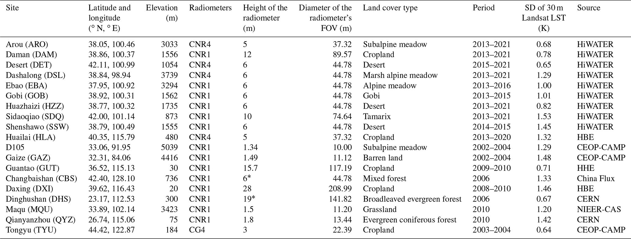
∗ This height is the instrument's average height above the tree canopy. The ground sites were operated by different field campaigns or programs. CERN: Chinese Ecosystem Research Network (Fu et al., 2010; Pastorello et al., 2020); CEOP-CAMP: Coordinated Energy and Water Cycle Observation Project (CEOP) and Asia–Australia Monsoon Project (CAMP) (Ma et al., 2006; Liu et al., 2004); China Flux (Pastorello et al., 2020; Yu et al., 2014; Zhang and Han, 2016); HHE: HaiHe Experiment in the Hai River Basin, China (Guo et al., 2020; S. M. Liu et al., 2013); HiWATER: Heihe Watershed Allied Telemetry Experimental Research (Che et al., 2019; X. Li et al., 2013; Liu et al., 2011, 2018, 2023); NIEER-CAS: Northwest Institute of Eco-Environment and Resources, Chinese Academy of Sciences (Wen et al., 2011). The datasets from HiWATER and HHE were downloaded from the National Tibetan Plateau Data Center (TPDC) (https://data.tpdc.ac.cn/, last access: 8 January 2024). The datasets from China Flux and CERN were downloaded from the China Flux Network (http://www.chinaflux.org/, last access: 8 January 2024); the datasets from CEOP-CAMP were downloaded from the Earth Observing Laboratory of the National Center for Atmospheric Research (https://data.eol.ucar.edu/dataset/, last access: 8 January 2024), and the dataset of MQU was downloaded from the link at http://tpwrr.nieer.cas.cn/, last access: 8 January 2024.
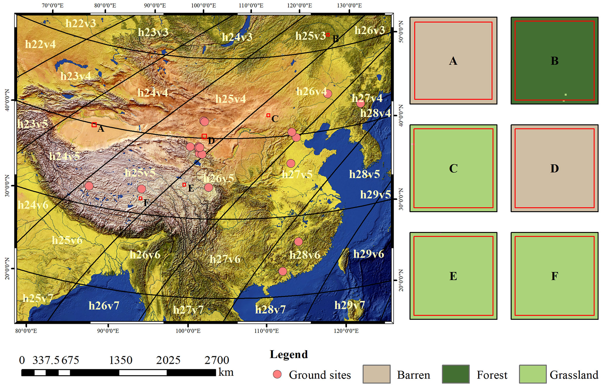
Figure 1The study area and the selected 19 ground sites. A, B, C, D, E, and F are subareas exhibiting a single land cover type with no change in T1 and T2 (1 January 2000 to 3 January 2005).
2.2 Ground measurements
Table 1 shows 19 ground sites that recorded longwave radiation data for different periods. According to the geographical locations and land cover types provided in Table 1, it is clear that they are distributed in different climate zones. This indicates that they encompass a wide range of land surface and climatic situations for sufficient validation of the TRIMS LST. The measurement device at the selected ground station includes a longwave radiometer and four-component radiometers, including CNR1, CNR4, and CG4 (Kipp & Zonen, Netherlands; https://www.kippzonen.com/, last access: 8 January 2024). According to the specifications of these radiometers, the uncertainties in the daily total for longwave radiation measurements are 3 %–10 % (Wang et al., 2020). With the measured incoming and outgoing longwave radiation, the LST of the land cover type within the field of view (FOV) of the radiometer can be calculated through the radiative transfer equation in the form of the Stefan–Boltzmann law (Ma et al., 2023, 2021). Considering the uncertainties in the longwave radiation measurement, the uncertainties in the calculated in situ LST are approximately 0.6–1.20 K (Xu et al., 2013; Yang et al., 2020; Ma et al., 2021).
Spatial representativeness of ground sites has different degrees of influence on the validation of TIR-based LST using in situ LST. In this study, to quantify the spatial representativeness, we calculated the standard deviation (SD) of 33 × 33 Landsat LST within MODIS pixels containing ground sites. Specifically, the Landsat LST is the 30 m Landsat-7 ETM+ Collection 2 Level-2 LST provided by the United States Geological Survey (U.S. Geological Survey, 2021). For the 19 sites, the SD ranged from 0.64 to 1.53 K, indicating good to acceptable representativeness of these sites for the validation of a 1 km LST (Zhang et al., 2021; Duan et al., 2019). Abnormal measurements, caused by short-term disturbances such as instantaneous shadow from small clouds and birds, were excluded from the ground-measured longwave radiation through a quality check. This quality check involved removing the outgoing or incoming longwave radiation that deviated by more than 3σ (standard deviations) from its respective 1 h averages (Göttsche et al., 2016).
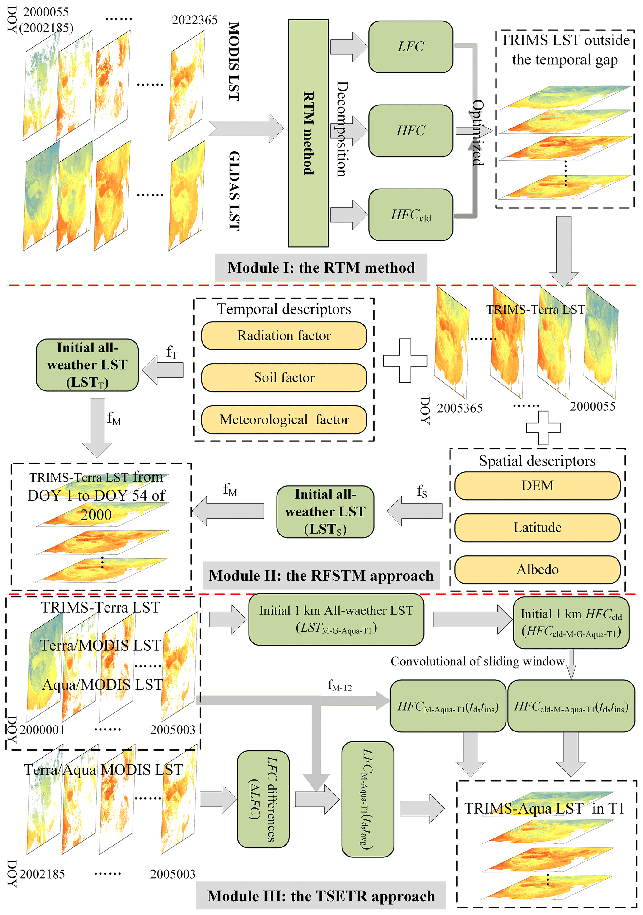
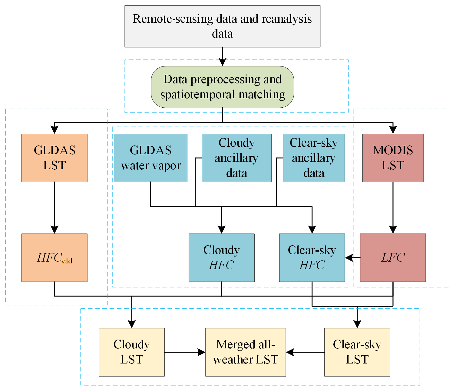
Figure 2Flowchart of the E-RTM method. Note that the date in this figure is in the format of YYYY + DOY.
The TRIMS LST was generated through the E-RTM method, consisting of the three modules depicted in Fig. 2. Module I runs the original RTM method (Zhang et al., 2021) to merge MOD11A1 (MYD11A1) and the GLDAS LST, producing daily all-weather LST at the Terra (Aqua) satellite overpass time from DOY 55 of 2000 (DOY 185 of 2002) to DOY 365 of 2022. Module II employs a random-forest-based spatiotemporal merging (RFSTM) approach to extend the beginning date of the MOD11A1 LST-based all-weather LST to 1 January 2000. Finally, Module III utilizes a time-sequential LST-based reconstruction (TSETR) approach to extend the beginning date of the MYD11A1 LST-based all-weather LST to 1 January 2000.
3.1 Module I: the RTM method
Details of the RTM method can be found in Zhang et al. (2021). For the convenience of the readers, a brief description of the RTM is provided here. In the temporal dimension, the time series of the LST can be expressed as
where td is the day of the year (DOY); tins is the overpass time of a satellite TIR sensor (i.e., MODIS) and tavg is the average observation time calculated from tins; LFC is the low-frequency component that represents the intra-annual variation component of the LST under ideal clear-sky conditions; HFC is the high-frequency component, which represents the sum of the diurnal LST variation and the weather variation component (WTC) under ideal clear-sky conditions; HFCcld is a correction term representing the impact on LST triggered by cloud contamination under cloudy conditions; and HFCcld is equal to zero under clear-sky conditions.
In the RTM method, LFC, HFC, and HFCcld in Eq. (1) are first determined from the MODIS LST and the GLDAS LST. Then, the optimized models are determined for the three components according to their characteristics, and their quality is improved by inputting their descriptors. Finally, three optimized components are integrated to generate the all-weather LST.
3.2 Module II: the RFSTM approach
The RFSTM approach was developed to predict the all-weather LST during the period of DOY 1–54 2000, during which the Terra MODIS LST was not available. It is based on the fact that (i) the LST of a pixel in the temporal dimension is strongly affected by the meteorological conditions as well as the underlying surface and that (ii) the LST of many pixels at a certain time are closely related to their underlying surfaces (Ma et al., 2021). Therefore, RFSTM has two stages, i.e., the temporal stage and the spatial stage.
At the temporal stage, the daily LST (LSTT) of a pixel Q in a certain period is modeled as
where the subscript T denotes the temporal stage, the function fT expresses the mapping in temporal dimensions from the descriptors to LST, XT denotes the matrix including the LST descriptors' time series (PT,i, ), and n is the number of days within the temporal gap of the Terra MODIS LST.
We used the mapping function fT to predict the 1 km all-weather LST, since the MODIS LST is not available as a reference for reconstruction and it is impossible to identify the different weather conditions (e.g., clear-sky and cloudy conditions). However, the relationship between LST and its descriptors cannot be analytically expressed currently. Fortunately, machine learning has been reported as effective in enhancing the spatial resolution of remote sensing images. Specifically, the random forest (RF) algorithm has shown good performance in mapping the correlation between LST with finer resolution and its descriptors with coarser resolution (Xiao et al., 2023; B. Li et al., 2021; Xu et al., 2021; Zhao and Duan, 2020; Yoo et al., 2020). Therefore, the RF algorithm was employed here to realize fT. The temporal descriptors of LST include the net longwave radiation, downwelling longwave radiation, soil moisture or temperature profile (e.g., surface, 0–10 cm, and 10–40 cm in GLDAS NOAH model-based data), canopy surface water, snow depth water equivalent, surface skin temperature, wind speed, and air temperature. The training period for fT with RF was set as DOY 55 of 2000 to DOY 55 of 2005, and the prediction period for LSTT was from DOY 1 of 2000 to DOY 55 of 2000.
Considering that LST varies in both spatial and temporal dimensions, the spatial descriptors of LST should also be considered. In the spatial stage, the LST (LSTS) at td in the prediction period is expressed as
where the subscript S denotes the spatial stage, the function fS expresses the mapping in spatial dimensions from the descriptors to LST, k is the number of spatial descriptors of LST, and NS denotes the 1 km spatial descriptor of LST (NS,i, ).
The spatial descriptors of LST include the DEM, latitude, and albedo. The selected descriptors in the spatial stage are all from the ancillary data with a 1 km resolution. Albedo serves as a descriptor that informs about land surface, including factors such as vegetation growth, surface or subsurface moisture distribution, and land surface cover type. We used GLASS albedo data as a substitution in the prediction step to fill the temporal gaps in MODIS LST because these temporal gaps are also effective in other MODIS products (including the MODIS albedo). Specifically, the GLASS albedo data are the best substitution for MODIS albedo data that we can find since they are strongly correlated with each other and have close accuracies according to existing studies (He et al., 2014; Wang et al., 2014; Chen et al., 2020; Lu et al., 2021).
To involve all the spatiotemporal LST descriptors and to guarantee the best performance of the output, the LSTs (LSTT and LSTS) need to be merged to derive the final 1 km LST (LSTM):
where fM denotes the RF-based mapping which indicates the contributions to the LSTM from LSTT and LSTS, respectively.
For a single 1 km pixel, the RF-based regression contribution function is trained using LSTT (obtained by Eq. 2), LSTS (obtained by Eq. 3), and TRIMS LST in the training period. Then, fC is applied to estimate the 1 km all-weather LST in the prediction period via Eq. (4).
3.3 Module III: the TSETR approach
The TSETR approach was developed to estimate the all-weather LST during the period from DOY 1 of 2000 to DOY 184 of 2002, during which the Aqua/MODIS LSTs were not available (with a temporal gap of 915 d). Previous studies have shown that it is possible to convert between the Terra/MODIS LST and the Aqua/MODIS LST, considering land cover types, geolocations, and seasons (Coops et al., 2007). Therefore, the Terra/MODIS LST from 2000 to 2002 could be transformed into the Aqua/MODIS LST (Li et al., 2018). Since the Terra/MODIS LST (MOD11A1) is available as a reference in the temporal gap, we generated an all-weather LST based on the TSETR approach, which is reconstruction rather than prediction.
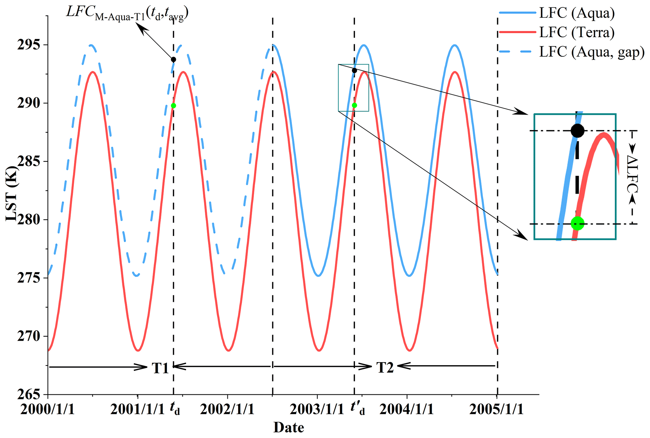
According to Eq. (1), the LST time series can be decomposed into LFC, HFC, and HFCcld under all-weather conditions. Therefore, the TSETR approach has three stages. In the first stage, we need to estimate the LFC during the temporal gap at the Aqua overpass time. In this case, the temporal gap period was set as T1, and DOY 185 of 2002 to DOY 3 of 2005 were set as T2 (Fig. 3). According to the analytical expression and physical meaning of LFC, there are no underlying trends of change within the three annual parameters (Tavg, A, and ω), except for the periodic variation in the LST, which means that the LFC is cyclic-stationary over a short period (Bechtel, 2015; Weng and Fu, 2014; Zhu et al., 2022). Once the three annual parameters are determined, the LFC can be calculated for a given day.
Therefore, in the TSETR approach, we assume that the LFC differences (ΔLFC) between the Terra and Aqua overpass times in T1 and T2 are also cyclic-stationary. In T2, the LFC values at the Terra/MODIS and Aqua/MODIS pixels are determined separately. In T1, the LFC at the Aqua overpass time of the pixel M can be expressed as
where td is a specific day in T1; is a specific day corresponding to td in T2; LFCM-Aqua-T1(td,tavg) and LFCM-Terra-T1(td,tavg), respectively, denote the LFC corresponding to the Aqua or Terra overpass time in T1; and LFC and LFC, respectively, denote the LFC corresponding to the Aqua or Terra overpass time in T2.
HFC is estimated in the original RTM method using a nonlinear mapping established by multiple descriptors. In the second stage of E-RTM, the HFC within T1 at the Aqua overpass time can be estimated by using its descriptors through RF (Xu et al., 2021). With Modules I and II, we have obtained the TRIMS-Terra LST in T1. However, it is unfeasible to directly model an RF mapping based on the Terra/MODIS LST and its corresponding descriptors in T1. An important concern that needs to be addressed is the timing discrepancy between Terra and Aqua observations, which results in distinct variations in the pattern of LST changes. When there is no valid Aqua/MODIS LST available, we have made improvements to the procedure for calculating the HFC in the original RTM method as follows:
where ΔLFC characterizes the systematic deviation of the steady-state component; gM is the geospatial code (Yang et al., 2022); DEMM, NDVIM, slpM, αM, ΔtM, and vM are the DEM, NDVI, slope, albedo, difference between tins and tavg, and atmospheric water vapor content, respectively; ΔDTC characterizes the warming effect of solar radiation; and the weather effect can be characterized by the atmospheric water vapor content. According to Zhang et al. (2021), the HFC characterizes the change in LFC with ΔDTC and WTC superimposed under ideal clear-sky conditions. The detailed calculation of ΔDTC can be found in Zhang et al. (2019b).
fM-T2 is constructed as follows. Initially, the correlation image of the target pixel M is determined within the T2 period, and the following two conditions need to be satisfied by the correlation image: (i) the mean bias deviation (MBD) of the DTC estimated from its corresponding GLDAS LST (10:00–14:00 and 21:00–03:00 local solar time) should be lower than 1 K, and (ii) the difference in the average observation time between the GLDAS pixels should not exceed 0.5 h. Using the correlation image, the similar image family S of the target pixel M is determined. Subsequently, in the correlation image, using similar land cover type criteria, the similar image family S of the target pixel M within the GLDAS pixels is identified. S needs to meet the following two conditions: (i) it should have the same land cover type as M, and (ii) the R of the Terra/MODIS LST time series corresponding to S and M needs to be greater than 0.8.
In the third stage, we need to estimate the HFCcld within the temporal gap period at the Aqua overpass time. HFCcld is essentially an atmospheric correction term, and it is obtained from the GLDAS LST in the RTM method. According to the parameterization scheme of the RTM method, the clear-sky MODIS pixels and their corresponding GLDAS LST are the necessary inputs for the estimation of HFCcld. It is not possible to obtain HFCcld directly at this stage due to the lack of Aqua/MODIS in T1.
Inspired by the temporal component decomposition (TCD) method (X. Zhang et al., 2019) and other methods integrating PMW and TIR LST (Parinussa et al., 2016; Zhang et al., 2020a), the initial value of the 1 km HFCcld can be expressed as
where HFCcld-M-G-Aqua-T1 is the initial 1 km HFCcld of M, and LSTM-G-Aqua-T1 is the initial 1 km LST of M under all-weather conditions.
Based on the findings of Yao et al. (2023), we established the method for acquiring the initial 1 km all-weather LST. Initially, the GLDAS LST that corresponded to the Aqua overpass time is corrected for systematic bias using the cumulative distribution function matching (Xu and Cheng, 2021). In the T1 period, since Aqua/MODIS LST is unavailable, we employed MODIS LST from 2003 to 2022 to guarantee an adequately large sample size of MODIS LST. We then downscaled the GLDAS LST to 1 km through the following two steps.
- i.
Calculating the LST differences between the MODIS and GLDAS:
where LSTG-Aqua-T1 is GLDAS LST, LSTM-Aqua-T1 is the ideal MODIS clear-sky LST, and LSTM-G-Aqua-T1 is an LST difference image. One pixel in GLDAS LST corresponds to 625 (25 × 25) pixels in MODIS LST. The LST differences are calculated as GLDAS LST minus the 625-pixel average MODIS LST. The LST difference image was then directly resampled to 1 km.
- ii.
Downscaling of GLDAS LST:
where LSTM-G-Aqua-T1 is the initial 1 km downscaled GLDAS LST. The heterogeneity of the underlying land surface within a 0.25∘ grid is reflected by MODIS LST, and the downscaled GLDAS LST also exhibits the same characteristic. This is based on the hypothesis that the spatial variations in MODIS LST are the same as those of GLDAS LST. However, LSTM-G-Aqua and HFCcld-M-G-Aqua-T1 in the results of Eq. (9) may still contain systematic errors due to inadequate downscaling (Eq. 8). Therefore, a convolutional implementation of a sliding window was used here to reduce the systematic error contained in HFCcld-M-G-Aqua-T1 (Chen et al., 2011; Wu et al., 2015; X. Zhang et al., 2019).
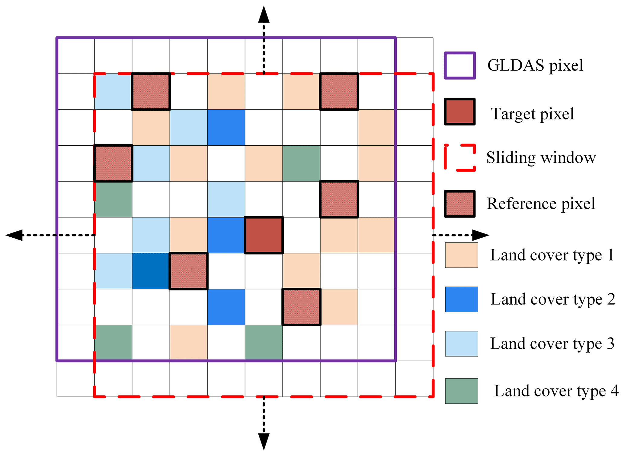
The schematic diagram of the convolutional implementation of the sliding window is shown in Fig. 4. To fully reduce the systematic bias, the size of the sliding window should be slightly larger than a GLDAS pixel (26 km × 26 km). According to Zhang et al. (2019b, 2021), HFCcld after optimization of M (i.e., HFCcld after eliminating the systematic errors) can be obtained by convolving the HFCcld of the surrounding similar pixels by combining geological factors (e.g., land cover type, spatial distance, and topography). This method is based on the interrelationship of different LSTs: neighboring HFCcld are correlated in a limited spatial domain. Previous studies have shown that the approaches analogous to the convolutional implementation of sliding windows have a good ability to improve both the accuracy and the image quality of the merged LST (Ding et al., 2022; Long et al., 2020; X. Zhang et al., 2019). Similar pixels (termed S) need to meet the following criteria: (i) they should be within the same sliding window as the target pixel, and (ii) their land cover type should not differ from the target pixel. Therefore, the target pixel itself is also a reference pixel. Eventually, the HFCcld of the target pixel can be expressed as
where n is the number of similar pixels; HFCcld-S denotes HFCcld-M-Aqua-T1 of the similar pixels; and ws is the contribution of similar pixels to M, which can be expressed as
where DS, HS, and NS are the differences between the similar pixels and M in terms of the spatial distance, DEM, and NDVI, respectively.
3.4 Implementation of E-RTM
A detailed description of the implementation process of the RTM method is provided by Zhang et al. (2021), and it is only briefly described in this section. Here, the implementation of Modules II and III is explained in detail.
Stage I: data preprocessing and spatiotemporal matching
In this stage, the data are preprocessed with spatiotemporal matching. First, valid MODIS LSTs are selected with the following two standards: (i) the quality control of the pixel was flagged as “good”, and (ii) the view angle of the pixel was lower than 60∘. Second, the selected temporal descriptors from GLDAS data were temporally interpolated using the cubic spline function to observe the time of MODIS LST for temporal matching. Third, the observation times for cloudy pixels and temporal gaps were recovered using a 16 d revisiting period. Fourth, the 90 m DEM, 500 m albedo, and 500 m NDSI were upscaled to 1 km to match the MODIS LST. Fifth, the GLDAS water vapor was extended to 1 km by cubic convolution interpolation. During the temporal gap (DOY 1–54 in 2000), SPOT VGT served as the NDVI, GLASS albedo was extended to a 1 km resolution using cubic convolution interpolation, and the NDSI was determined by taking the average of the corresponding days in 2001 and 2002. The 16 d 1 km NDVI is temporally interpolated to daily resolution. The daily missing albedo caused by the cloud is filled up through Statistics-based Temporal Filter (N. F. Liu et al., 2013). In addition, all the data are spatially matched.
Stage II: implementation of the RTM
- i.
For the target MODIS pixel, its annual-scale LST time series are extracted and fitted to obtain the LFC component.
- ii.
The HFC components of all comparable pixels are estimated.
- iii.
To create a mapping model of the HFC components and the corresponding spatial descriptors, a machine-learning approach is implemented.
- iv.
The trained mapping model is utilized to determine the HFC under clear-sky conditions.
- v.
Bias-correct the GLDAS LST to match that of the MODIS LST.
- vi.
Calculate the HFCcld present in the GLDAS LST.
- vii.
Estimate the HFCcld of the target pixel.
- viii.
Achieve the estimation of LST under clear-sky conditions (LFC + HFC).
- ix.
Implement the estimation of LST under cloudy conditions (LFC + HFC + HFCcld).
- x.
Repeat the above steps for every pixel of MODIS LST to achieve the fusion of TIR LST and GLDAS LST.
Stage III: implementation of the RFSTM
- i.
For a single 1 km pixel, train the RF regression relationship (i.e., fT) between TRIMS-Terra LST and the temporal descriptors from GLDAS data via Eq. (2). The RF parameters were set as follows: n estimators = 85, maximum depth = 18, maximum features = 3, and minimum leaf samples = 1. In the temporal stage of RFSTM, all-weather samples from 2000 to 2005 were compiled. Two-thirds of the samples are used for model training, and the rest are for model validation (Breiman, 2001).
- ii.
For a specific day (td), use the 1 km NDVI (Sobrino et al., 2004) and NDSI to classify the study area into several subareas, including thick vegetation (NDVI > 0.5), sparse vegetation (0.2 ≤ NDVI ≤ 0.5), barren land areas (NDVI < 0.2), snow ice areas (NDSI > 0.1) (H. Zhang et al., 2019), and water (NDVI < 0). Then, for each subarea, the spatial descriptors of LST are input into fS via Eq. (3). The RF parameters were set as follows: n estimators = 420, maximum depth = 43, maximum features = 9, and minimum leaf samples = 1. Note that fS with RF is trained with the 1 km LST and spatial descriptors of a day, with the same observation time as td and the smallest difference in the number of days between td.
- iii.
For a single 1 km pixel, train the RF-based regression contribution function (i.e., fM in Eq. 4) using LSTT, LSTS, and TRIMS-Aqua LST under clear-sky conditions. Then, estimate the 1 km TRIMS-Aqua LST during the period of DOY 1–54 in 2000 by applying fM to clear-sky and cloudy conditions, respectively.
Stage IV: implementation of the TSETR
- i.
For a single Aqua/MODIS pixel M in T1, determine its LFC in Eq. (5) using Aqua/MODIS LST (T2) and Terra/MODIS LST (T1 and T2).
- ii.
Train the RF measurement (fM-T2) between all of the ΔHFC and its descriptors (see Sect. 3.3) of all similar pixels. The RF measuring function tools are also provided by the MATLAB platform. The RF parameters were set as follows: n estimators = 100, maximum depth = 20, maximum feature = 4, and minimum leaf samples = 1. Determine the reconstructed HFC of M through Eq. (6) by applying the descriptors of HFC in M to fM-T2.
- iii.
Implement the bias correction for GLDAS LST of the target GLDAS grid by using cumulative distribution function matching. Then, downscale the GLDAS LST to 1 km through Eqs. (8) and (9).
- iv.
Determine the initial 1 km HFCcld of M through Eq. (7). Finally, determine the HFCcld of M through Eqs. (10) and (11).
3.5 Evaluation strategies
As can be seen from Fig. 2, TRIMS LST can be divided into two parts according to the period of data coverage: data within the temporal gap period and data outside the temporal gap period. There are differences in the evaluation strategies within the two periods due to the different availabilities of validation data.
For outside the temporal gap period, the TRIMS LST was compared with LSTs derived from two reanalysis datasets (i.e., GLDAS and the independent ERA5-Land) and retrievals from two different satellite TIR sensors (i.e., MODIS and the independent AATSR). In comparing different LSTs, samples with time differences greater than 5 min were excluded (Freitas et al., 2010; Göttsche et al., 2016; Jiang and Liu, 2014). The quantitative metrics used in the comparison analyses include the MBD, the SD of the bias, and the coefficient of determination (R2). Then, the TRIMS LST was validated under different weather conditions based on in situ LST from the ground sites listed in Table 1. The three metrics used are the MBE, RMSE, and R2.
During the temporal gap period, the TRIMS LST was tested using three methods. Firstly, the results of the original RTM method were cross-referenced and validated empirically with RFSTM and TSETR. In 2003, RFSTM was utilized to merge GLDAS LST and Terra/MODIS LST, resulting in a 1 km all-weather LST. Additionally, the TSETR method was employed to generate TRIMS-Aqua LST for the periods of 2003–2005 and 2013–2015. For the actual data generated for the period 2000–2002, specifically Aqua LST, the similarity of the TRIMS LST time series was quantified to examine the reliability of TRIMS LST during the Aqua/MODIS temporal gap. The time series angle (TSA), inspired by the spectral angle that is widely used to measure the similarity between spectral curves (Kruse et al., 1993), was used to quantify the similarity of the TRIMS LST time series. The TSA is defined as
where θ is the TSA (∘), and LSTTRIMS−Aqua and LSTTRIMS−Terra are time series of TRIMS-Aqua and TRIMS-Terra LSTs, respectively. From this formula, we know that a smaller TSA denotes higher similarity.
Based on the CLCD described in Sect. 2.1, six subareas with a single land cover type and no land cover change in T1 and T2 (1 January 2000 to 3 January 2005) were selected to extract the corresponding TRIMS-Terra and TRIMS-Aqua LST time series. These six subareas (Fig. 1) were recorded as A (82.30–83.16∘ N, 39.63–40.03∘ E; barren land), B (124.73–125.17∘ N, 51.51–51.95∘ E; forest), C (111.84–112.30∘ N, 42.47–42.85∘ E; grassland), D (100.78–101.53∘ N, 39.92–40.44∘ E; barren land), E (98.14–98.61∘ N, 33.92–34.25∘ E; grassland), and F (91.73–92.22∘ N, 31.7–32.01∘ E; grassland). Then, the TSA was calculated to quantify the similarity between the TRIMS-Terra and TRIMS-Aqua LST time series.
Finally, we evaluated the percentage of valid pixels in TRIMS LST and MODIS LST to prove the continuity of TRIMS LST during the temporal gaps. Furthermore, we analyzed the fluctuations in LST during the connectivity period (February and March 2000 for Terra, June and July 2002 for Aqua) to demonstrate the uninterrupted TRIMS LST sequence at the conclusion of the filled duration.
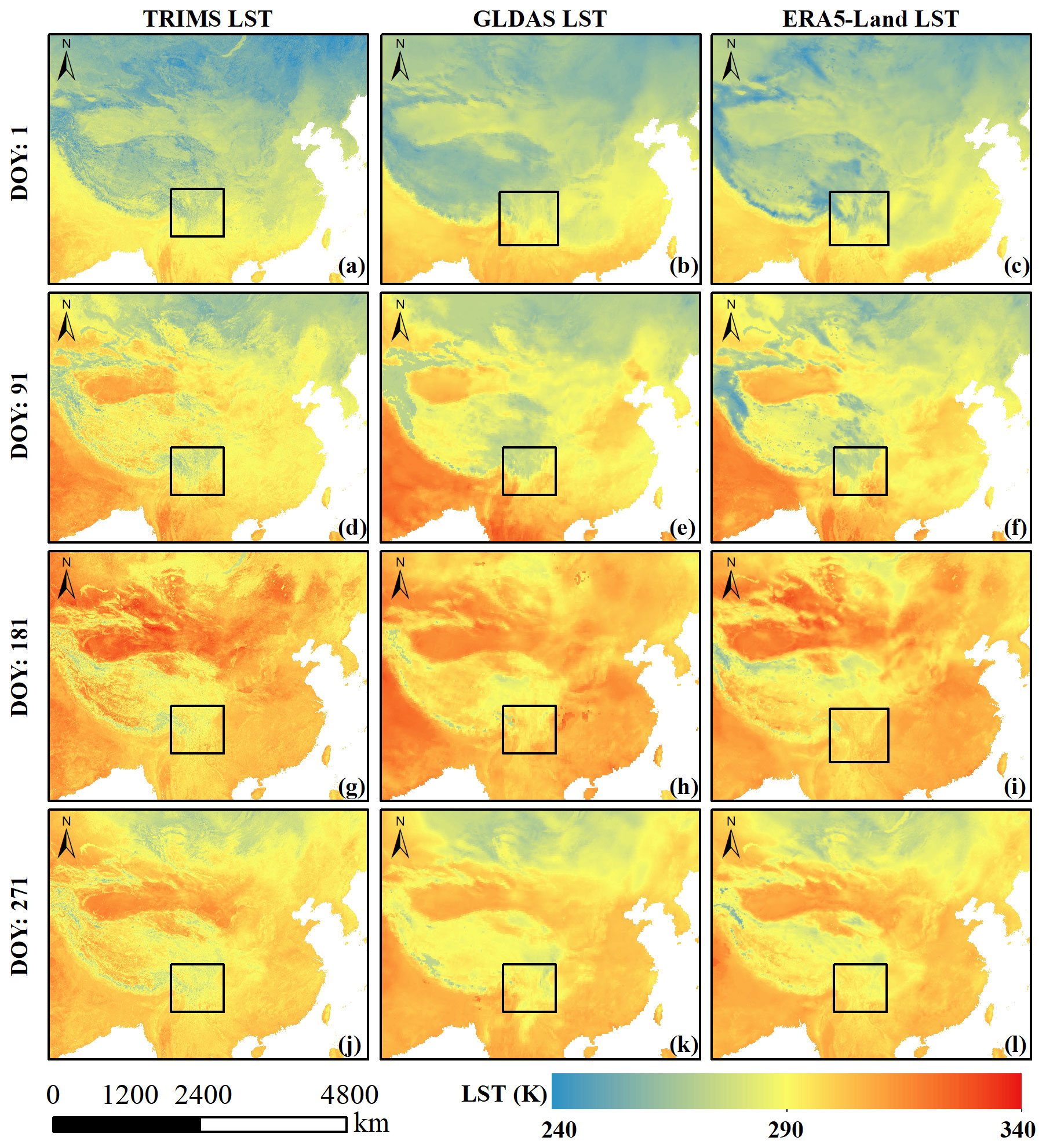
Figure 6Spatial patterns of the daytime TRIMS-Aqua LST, GLDAS LST, and ERA5-Land LST on 4 selected days in 2000.
4.1 Comparison of the TRIMS LST with reanalysis data
With the E-RTM method, TRIMS LST products from 1 January 2000 to 31 December 2022 were generated. The spatial resolution was 1 km. The temporal resolution was four observations per day, which is the same as with Terra/MODIS and Aqua/MODIS. Figure 6 shows the daytime TRIMS-Aqua LST on DOYs 1, 91, 181, and 271 as examples.
Figure 6 shows that the TRIMS-Aqua LST has a similar spatial pattern to the GLDAS LST since the latter is an input for the former. Good agreement in the spatial pattern in different seasons can also be observed between TRIMS-Aqua LST and the independent ERA5-Land LST. A careful observation of Fig. 6 demonstrates that the TRIMS LST is spatially seamless, and its spatial patterns are as expected. Southern China as well as Southeast Asia and the southern Asian subcontinent at low latitudes are warm in all the seasons because of additional absorbed solar radiation. The Tibetan Plateau, with a much higher elevation and regions at high latitudes, is much cooler than other regions. In winter (DOY 1), summer (DOY 181), and fall (DOY 271), northwestern China, where the dominant land cover type is barren land, is much warmer than other regions. Further comparison indicates that TRIMS LST is generally slightly warmer than the GLDAS LST and the ERA5-Land LST. For example, on DOY 1 of 2000, the LST is generally below 278 K on the eastern Tibetan Plateau, while the GLDAS LST and the ERA5-Land LST are approximately 3–5 K lower. In the generation scheme of the TRIMS LST, the MODIS LST, which is generally warmer than the LST provided by reanalysis data, is an important input as well as a reference to “calibrate” the GLDAS LST. This induces the “merged” TRIMS LST to be warmer than the GLDAS LST as well as the ERA5-Land LST.
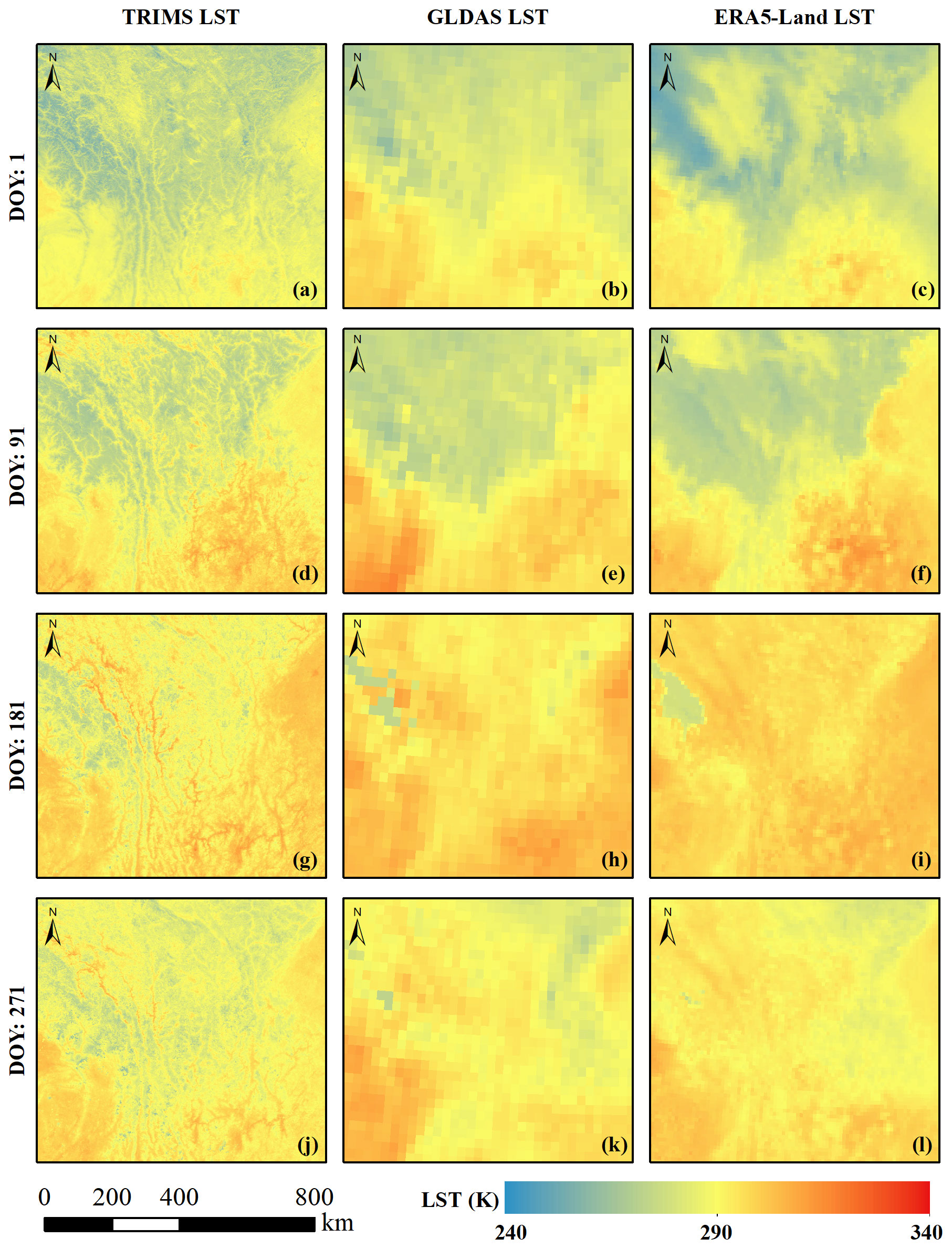
Figure 7The daytime TRIMS-Aqua LST, GLDAS LST, and ERA5-Land LST of the subarea (shown in Fig. 6) in 2000.
To further examine the image quality of the TRIMS-Aqua LST, Fig. 7 shows the daytime TRIMS-Aqua LST, GLDAS LST, and ERA5-Land LST of the subarea shown in Fig. 6 at the Aqua overpass time in 2000. Compared with the GLDAS LST and the ERA5-Land LST, the TRIMS LST offers more spatial details because of its much higher spatial resolution. Thus, one can see clear terrain-induced temperature variations. Furthermore, Fig. 7 shows that no evident spatial discontinuities exist in the TRIMS LST, indicating that the E-RTM method performs satisfactorily in addressing the spatial-scale mismatch between the MODIS LST and the GLDAS LST (Zhang et al., 2021).
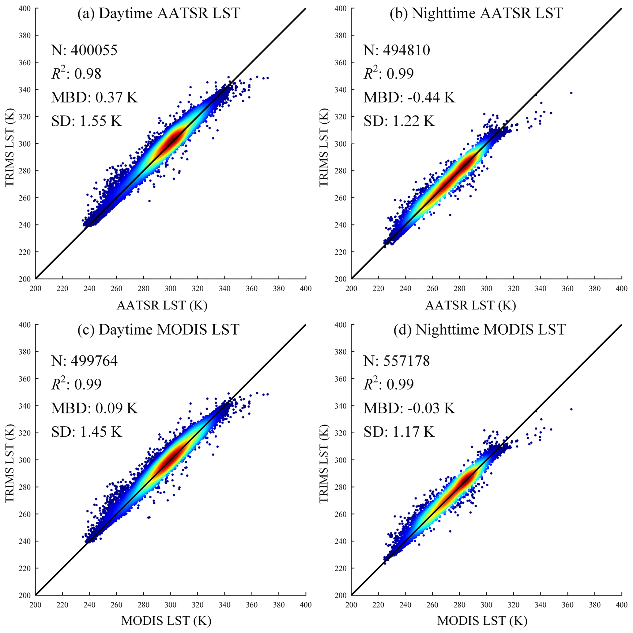
4.2 Comparison of the TRIMS LST with satellite TIR LST products
The daily TRIMS LST was compared with the independent ENVISAT/AATSR LST (from 2004 to 2012) and the Terra/Aqua MODIS LST (from 2000 to 2021 for Terra and from 2002 to 2021 for Aqua). Note that the AATSR and MODIS only have clear-sky LST. The density plots are shown in Fig. 8. To facilitate the data processing and presentation, 1 %/1 ‰ matched TRIMS-AATSR–MODIS pairs were randomly extracted. Figure 8 indicates good consistency between the TRIMS LST and AATSR/MODIS LST. Compared with AATSR, the overall MBD or SD values of TRIMS were 0.37/1.55 and −0.44/1.22 K for daytime and nighttime, respectively; compared with MODIS, the overall MBD or SD values were 0.09/1.45 and −0.03/1.17 K for daytime and nighttime, respectively. Figure 8 also shows that better agreements exist during nighttime because of lower thermal heterogeneity.
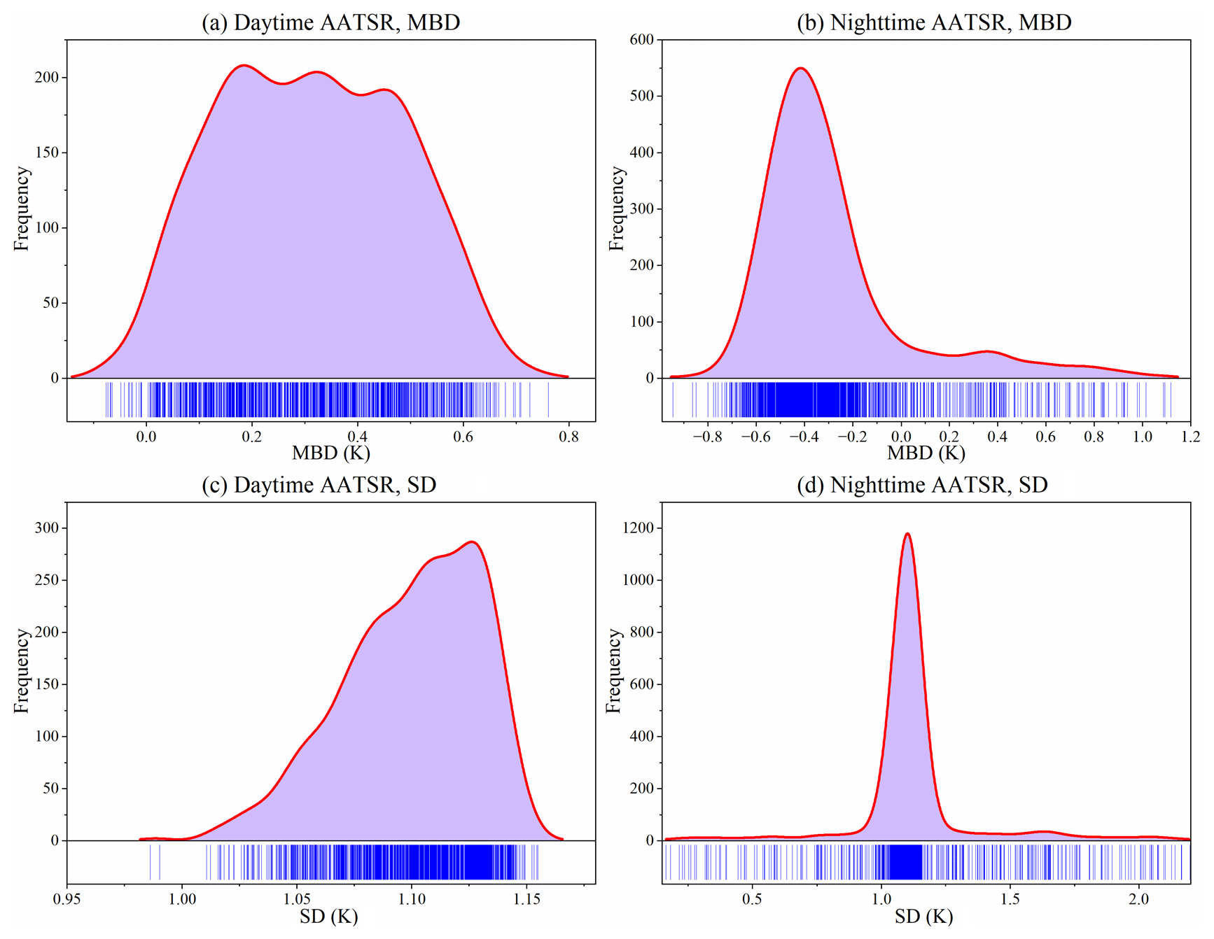
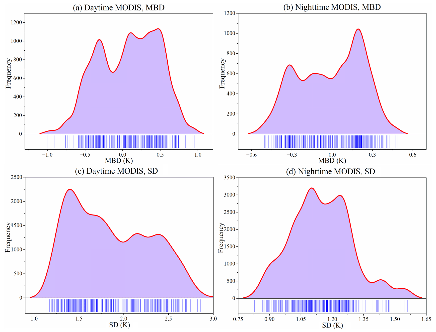
To further examine the deviation of the TRIMS LST from the AATSR/MODIS LST, the MBD and SD values were calculated for each day. Figure 9 shows the corresponding histograms. For AATSR, the daily daytime MBD and SD were mainly concentrated in the ranges of 0–0.60 and 1.05–1.15 K, respectively; the daily nighttime MBD and SD were mainly concentrated in the ranges of −0.40 to 1.0 and 0.75 to 1.15 K, respectively. The positive deviation and negative deviation were consistent with those in Fig. 9a and b. For the MODIS case, the daytime MBD was concentrated between −0.6 and 1.0 K, and the SD was concentrated between 1.0 and 2.50 K; the nighttime MBD was concentrated between −0.6 and 0.3 K, and the SD was concentrated between 0.9 and 1.50 K (Fig. 10). As shown above, it should be concluded that the daily differences between the long-term TRIMS LST and AATSR/MODIS LST remain stable.
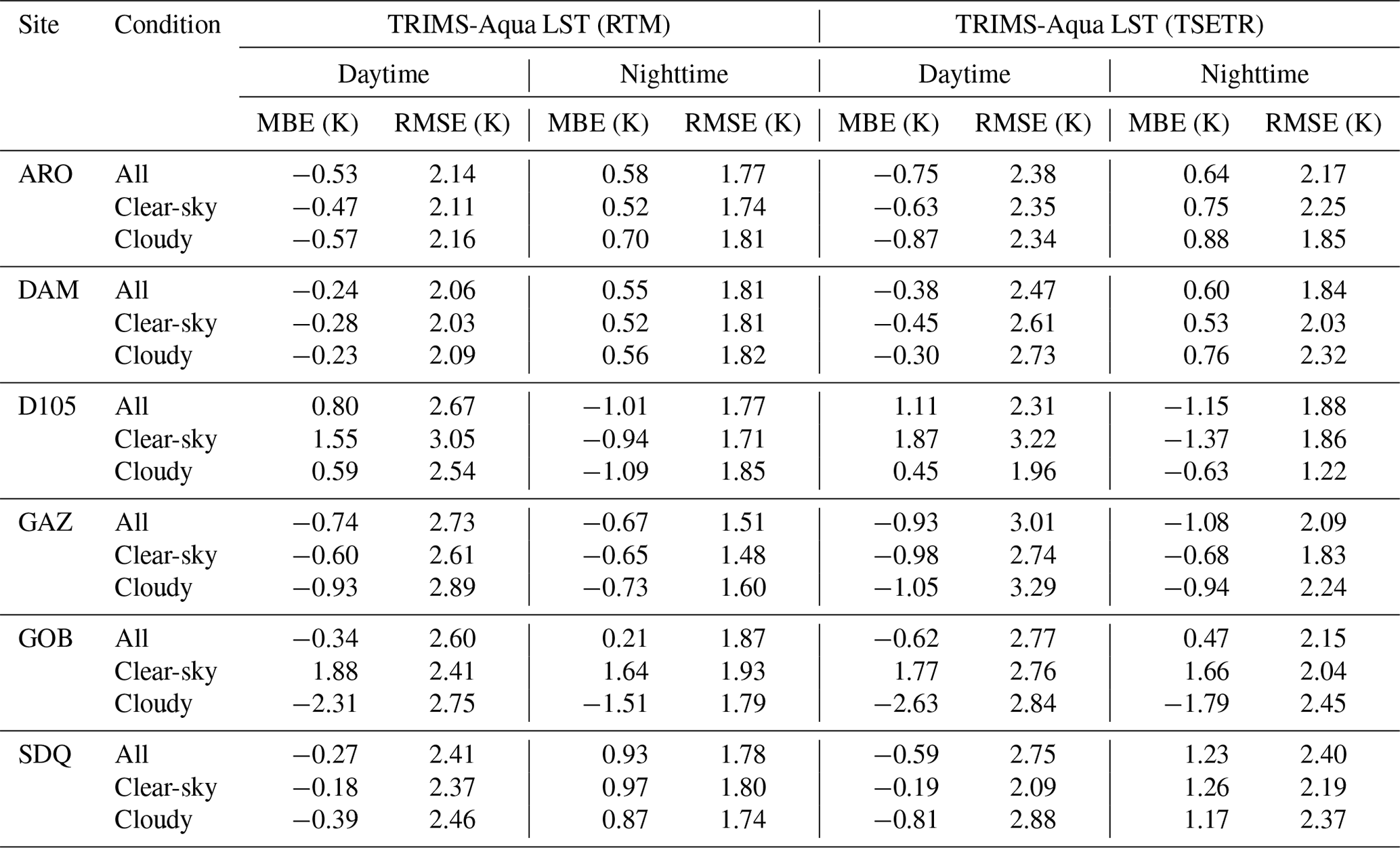
Table 2R2, MBE, and RMSE of the daytime validation for different groups.
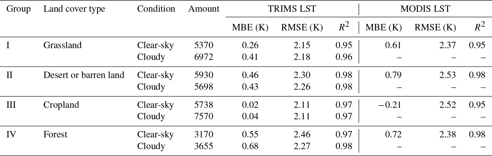
Table 3R2, MBE, and RMSE of the nighttime validation for different groups.
4.3 Validation against in situ LST outside the temporal gap
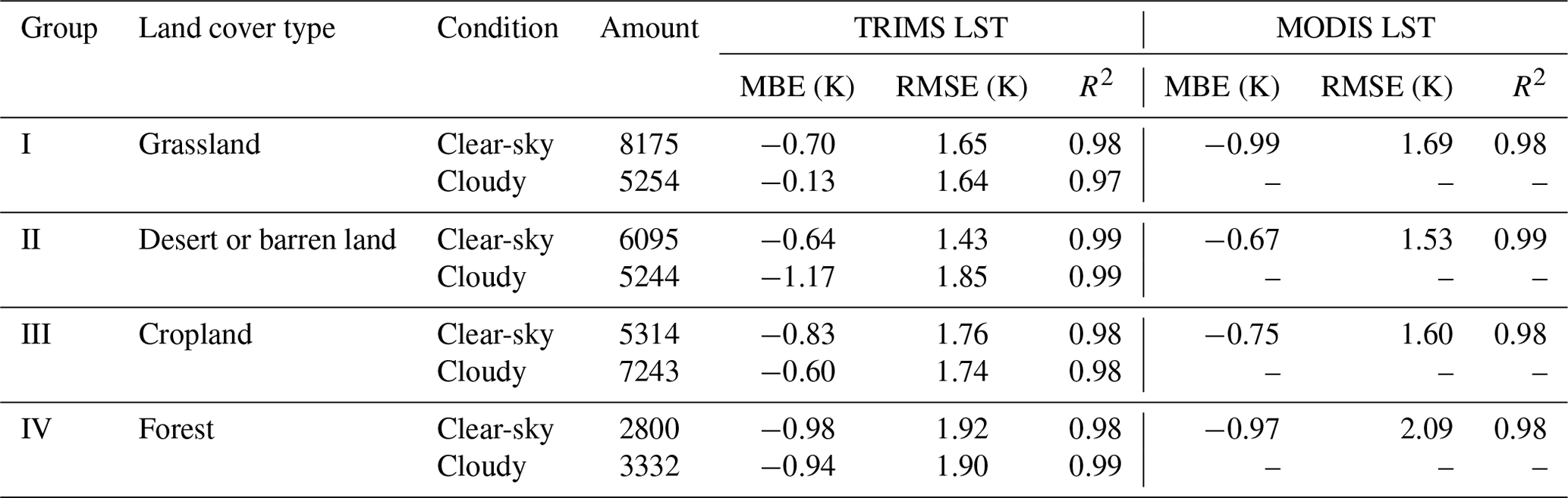
The TRIMS LST was quantitatively validated against the in situ LST. Anomalies arising from transient environmental factors were removed based on 3σ filtering (Göttsche et al., 2016; Yang et al., 2020). It should be noted that the results for all the sites can be found in Tables B1 and B2. The 19 ground sites were divided into four groups according to locations and land cover types (Group I: ARO, D105, DSL, EBA, and MQU; Group II: DET, GAZ, GOB, HZZ, and SSW; Group III: DAM, DXI, GUT, HLA, and TYU; Group IV: CBS, DHS, QYZ, and SDQ). Tables 2 and 3 show the validation results of TRIMS LST against the in situ LST under different sky conditions. In addition, the validation results of the clear-sky MODIS LST are provided for comparison.
Under clear-sky conditions, the TRIMS LST had an accuracy close to that of the MODIS LST as shown in Tables 2 and 3. The MBE of the TRIMS LST ranged from −0.98 to 0.68 K, and the RMSE was 1.43 to 2.46 K. The RMSE of the TRIMS LST under clear-sky conditions is lower than that of the MODIS LST, except for Group IV. The RMSEs of the MODIS LST were reduced by 0.22 K (Group I), 0.23 K (Group II), and 0.41 K (Group III), respectively. The nighttime results were generally better than the daytime results, with an average RMSE of 1.74 K. The R2 of the TRIMS LST for the four groups of sites was higher than 0.95 under clear-sky conditions, indicating that the TRIMS LST is in good agreement with the in situ LST. The improved accuracy of the TRIMS LST may be due to the reduction in the systematic bias of the original MODIS LST in the E-RTM method by extracting the LFC and HFC (Ding et al., 2022).
Under cloudy conditions, the accuracy of TRIMS LST is slightly lower compared to clear-sky conditions, resulting in a 0.35 K increase in the overall RMSE. For TRIMS LST under cloudy conditions, the accuracy is marginally below that under clear-sky conditions, and the overall RMSE increased by 0.35 K. For the four groups of sites, the MBE values of TRIMS LST were −0.13 K (Group I), −1.17 K (Group II), −0.60 K (Group III), and −0.94 K (Group IV), revealing that the TRIMS LST is underestimated under cloudy conditions. According to the parameterization scheme of the E-RTM method, the accuracy of the estimated HFCcld under cloudy conditions is affected by the GLDAS LST, which has a negative deviation from the MODIS LST as shown in Sect. 4.1. In contrast, although the GLDAS LST is bias-corrected, uncertainty may still exist, which is ultimately detrimental to the accurate recovery of the LST for the cloud-contaminated region. Overall, the validation results indicate that TRIMS LST has good accuracy under cloudy conditions as well as under clear-sky conditions.
For ground sites in Group III with a dominant land cover type of desert or barren land, the nighttime validation shows that the TRIMS-Aqua LST is systematically underestimated, with an MBE of −1.17 to −0.64 K. After checking the calculated SD, we believe that the spatial-scale mismatch between the ground site and the pixel is not the main reason for the systematic underestimation. Further examination shows that the clear-sky MODIS LST is significantly underestimated: the MBEs of Aqua/MODIS LST are −1.88, −1.03, −1.33, and −0.60 K for GOB, HZZ, SSW, and GAZ, respectively. Such a cold bias in arid and semiarid regions has also been reported by Li et al. (2019) for the MYD11 LST product. The above results indicate that the accuracy of TRIMS LST is largely dependent on the used MODIS LST.
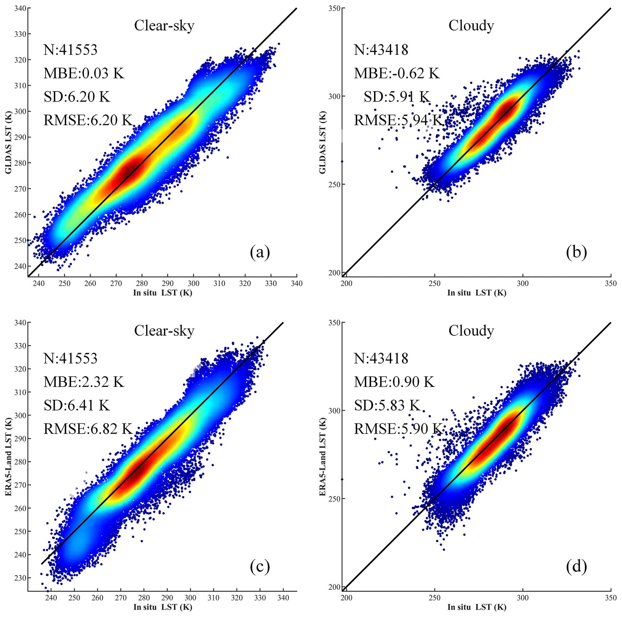
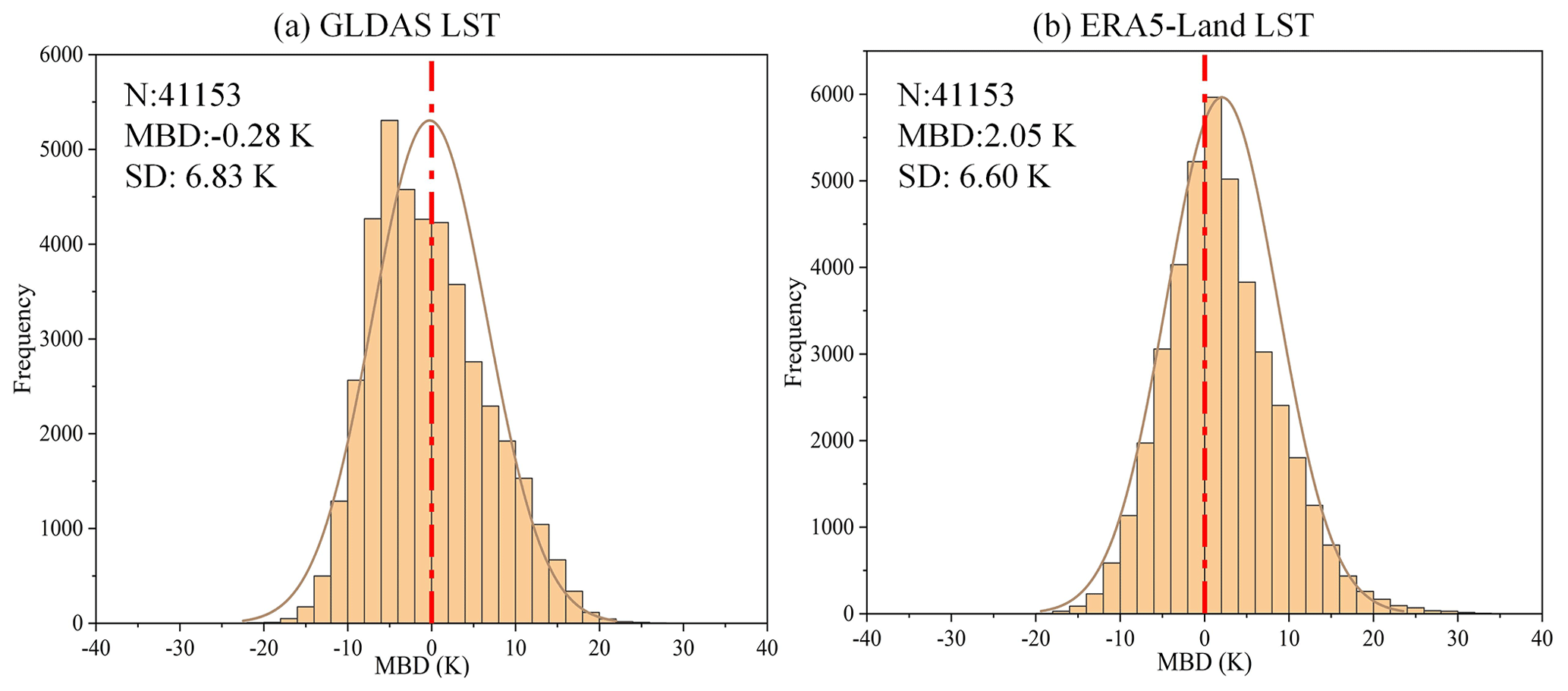
Reanalysis LST was also validated against in situ LST (Fig. 11). GLDAS LST is generally underestimated compared to in situ LST, with an MBE of −0.29 K and an RMSE of 5.86 K. Under clear-sky and cloudy conditions, the GLDAS LST exhibits MBE values of 0.03 and −0.62 K, respectively. On the other hand, ERA5-Land LST is overestimated compared with in situ LST, with an MBE of 1.60 K and an RMSE of 6.37 K. This indicates that the accuracy of the ERA5-Land LST is lower than that of the GLDAS LST. Notably, this discrepancy is more pronounced under clear-sky conditions. The results of the comparison with MODIS LST are shown in Fig. 12. GLDAS LST is underestimated relative to MODIS LST with a small deviation, while ERA5-Land LST is overestimated relative to MODIS LST with a large deviation.
Table 4MBE and RMSE from validation results of TRIMS-Terra LST with the in situ LST.
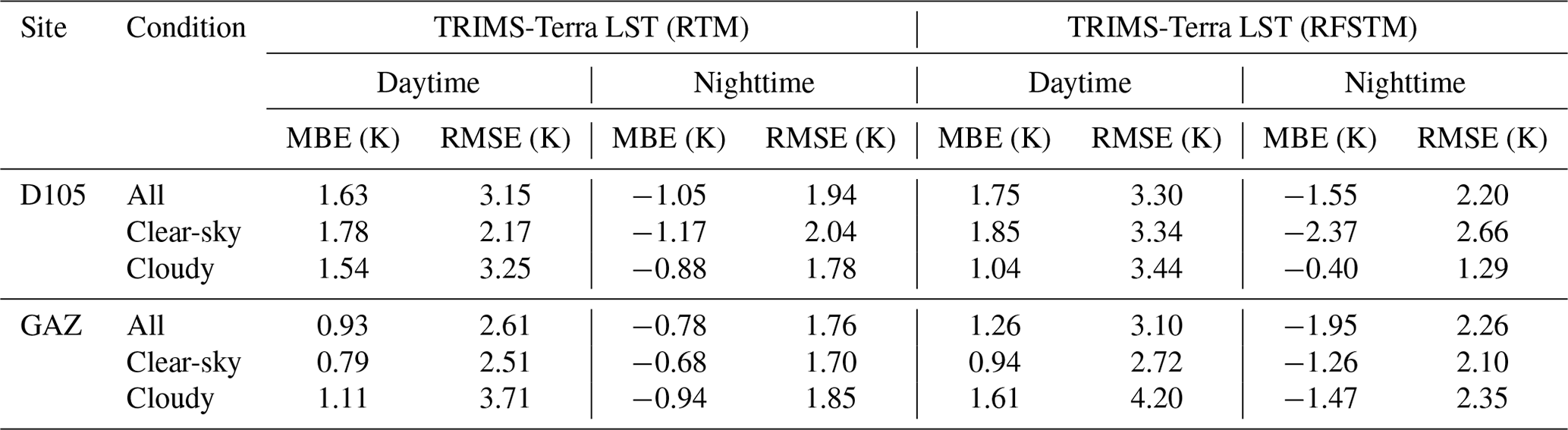
Table 5MBE and RMSE from validation results of TRIMS-Aqua LST with the in situ LST.
4.4 Validation of TRIMS-Aqua LST and TRIMS-Terra LST during the temporal gap
During the T1 period, there are no independent in situ LST measurements available. Observations of D105 and GAZ began on DOY 275 (2 October) of 2002. To investigate the generalization ability of the RFSTM in the temporal dimension, the method is implemented as follows. For 2003, the GLDAS LST and Terra/MODIS LST are also merged to generate 1 km TRIMS-Terra LST. This study utilized the TSETR method to reconstruct the TRIMS-Aqua LST over 915 d. To ensure a comprehensive analysis, TRIMS-Aqua LST for the years 2003 (DOY 1)–2005 (DOY 185) and 2013 (DOY 1)–2015 (DOY 185) were generated using the TSETR method. This allowed for the inclusion of a significant number of independent ground sites for validation purposes.
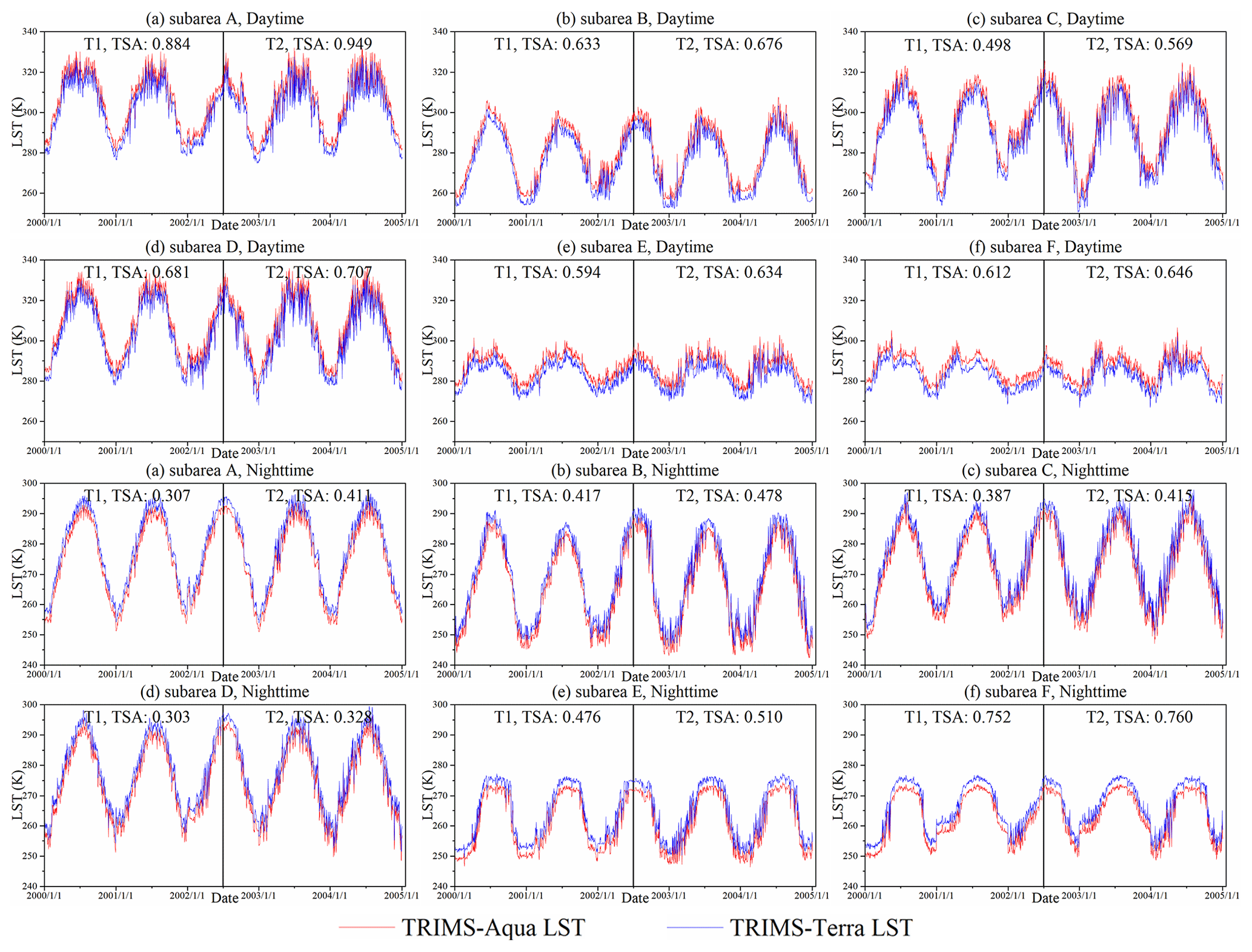
Figure 13TRIMS-Terra and TRIMS-Aqua LSTs from 1 January 2000 to 3 January 2005, together with statistics of the time series similarity.
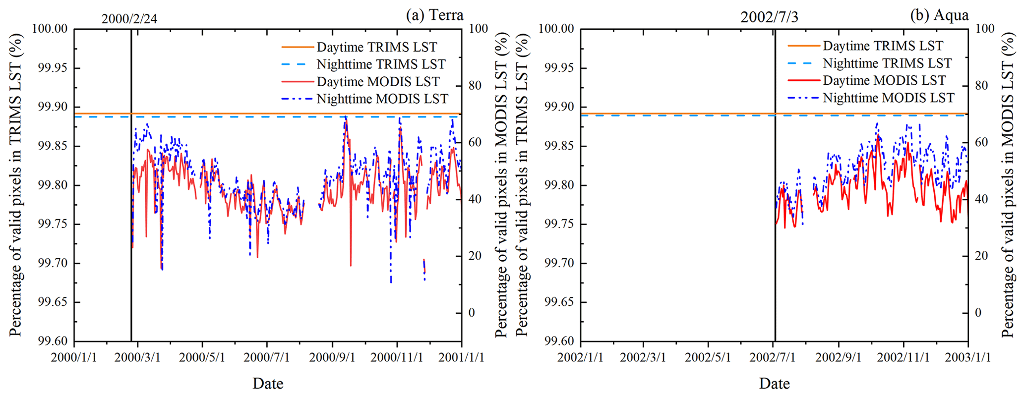
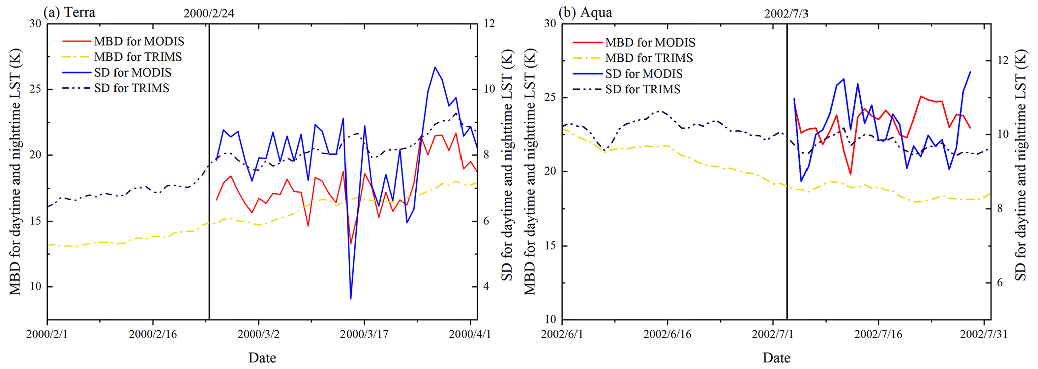
Table 4 shows the results of the comparison between the TRIMS-Terra LST generated by the RFSTM-based method and the TRIMS-Terra LST generated by the RTM-based method. The TRIMS-Terra LST generated by the RTM method and the TRIMS-Terra LST generated by the RFSTM method have similar accuracies for the sites. The MBEs differ by no more than 0.50 K, and the RMSEs differ by no more than 1.20 K. However, the RFSTM method is slightly less accurate than the TRIMS-Terra LST generated by the RTM method. It is important to note that the RFSTM method is only used in this study to generate data for 54 d, which has a relatively smaller impact on the overall accuracy of TRIMS LST.
Combining the results of Tables 4 and 5, it can be observed that the TRIMS-Aqua LST generated by the TSETR method and the TRIMS-Aqua LST generated by the RTM method exhibit similar accuracies at the sites. The differences in MBE and RMSE between these two methods are not significant, with the MBE differing by no more than 0.40 K and the RMSE differing by no more than 0.70 K. These findings demonstrate that the TSETR method maintains high accuracy and stability when generating data over longer periods. Based on this, it can be concluded that the TRIMS-Aqua LST in the T1 period reconstructed using the TSETR method is reasonably accurate.
Tables 4 and 5 demonstrate the reliability of RFSTM and TSETR. Figure 13 further shows the quantification results of the similarity between the TRIMS-Aqua LST and TRIMS-Terra LST time series during the temporal gaps. Overall, the trends in the time series of TRIMS-Terra and TRIMS-Aqua LST are very consistent, and they generally have a high degree of similarity. The daytime time series shows that the TRIMS-Aqua LST is generally higher than the TRIMS-Terra LST, while the opposite is observed for the nighttime. In particular, for subareas E and F, the TRIMS-Aqua LST shows a significant systematic deviation from the TRIMS-Terra LST during nighttime. The distribution of the curves in Fig. 13 reveals that the daytime LST time series had more large fluctuations, while the nighttime variation is more subdued. The TSA is lower at nighttime than at daytime, indicating that the time series similarity between the TRIMS-Aqua LST and the TRIMS-Terra LST is higher at nighttime. In addition, the TRIMS-Terra and TRIMS-Aqua LSTs are slightly more similar in T1 than in T2 among these six regions. This situation is as expected since the TRIMS-Aqua LST in T1 is derived from a mapping created by the data at the Terra overpass time. The differences in the TSA between T1 and T2 ranged from 0.0080 to 0.0710. The mean differences are 0.0465 (daytime) and 0.0433 (nighttime). The above results indicate that the similarity of the LST time series of T1 and T2 is relatively close. This finding demonstrates that the difference between TRIMS LST at the Aqua and Terra overpass times is stable in T1.
Meanwhile, we determined the percentage of valid pixels in TRIMS LST and MODIS LST, respectively (Fig. 14). The findings reveal that TRIMS LST is spatiotemporally continuous during the temporal gaps. The percentage of valid pixels in MODIS LST ranges from approximately 10 % to 70 %, exhibiting substantial seasonal fluctuations. The rise in water vapor, heightened convection, and increased cloud cover during summers could account for the reduced number of effective pixels. This condition also clarifies why, under most circumstances, fewer valid pixels are evident throughout the daytime than at nighttime. By comparison, the number of valid pixels in TRIMS LST changes moderately over time. Approximately 1 ‰ pixels were left unoccupied for a few days, likely due to the unavailability of reference groups and corresponding pixels within the search window during the determination of HFCcld for these pixels. However, the percentage of valid pixels almost reached 100 % following the combination of the RFSTM and TSETR approaches. This phenomenon is a quantitative demonstration of the success of the E-RTM method in recovering unspecified LSTs during the temporal gaps.
Finally, our analysis focused on examining the temporal variations in LST during the connectivity period (February and March 2000 for Terra, June and July 2002 for Aqua). The outcomes reveal that there is no interruption in the sequence at the conclusion of the filled duration (Fig. 15).
During the connectivity period, we calculated MBD and SD for daytime MODIS LST compared to nighttime MODIS LST. The MBD and SD for MODIS LST exhibited large fluctuations between dates, whereas the MBD and SD of TRIMS LST showed smoother overall trends with less fluctuation between dates. This is attributed to the consideration of the LFC as the primary base element in the E-RTM method, particularly during the temporal gap when valid MODIS LST data are lacking. The trends in MBD and SD for TRIMS LST and MODIS LST are generally consistent outside of the temporal gaps. Specifically, between 24 February and 31 March 2000, MBD and SD demonstrated a general upward trend, while between 3 and 31 July 2002, they showed an overall downward trend. Importantly, the trend of MBD and SD changes before and after the connecting dates is continuous without abrupt changes or breaks, as depicted in Fig. 15, indicating uninterrupted LST time series during the temporal gaps.
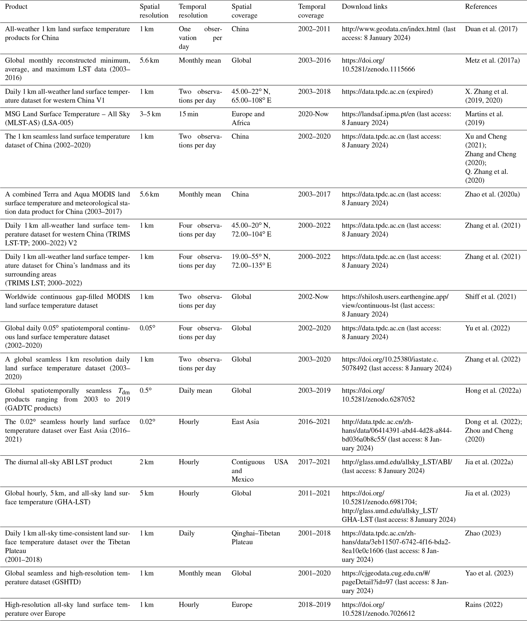
4.5 Advantages of the TRIMS LST
Recently, several all-weather LST datasets have been released by the scientific community (see Appendix C). An all-weather LST product series with a temporal resolution from 15 min (Martins et al., 2019) to monthly (Metz et al., 2017b; Zhao et al., 2020a; Hong et al., 2022b; Yao et al., 2023), a spatial resolution from 1 km to 0.5∘, and a spatial coverage from a specific region (Qinghai–Tibetan Plateau, China, Asia, Europe, and Africa) to the globe has been preliminarily formed. All-weather LST products based on MODIS LST interpolation (Zhang et al., 2022) or fusion with other multisource data (Xu and Cheng, 2021; Zhang and Cheng, 2020; Q. Zhang et al., 2020; Zhang et al., 2021; Yu et al., 2022) dominate the field. TRIMS LST similarly belongs to this group. Overall, the uniqueness or advantages of the TRIMS LST are in three main areas.
First, the TRIMS LST demonstrates comparable or better accuracy than existing publicly released all-weather or spatially seamless LST datasets. A thorough comparison with satellite TIR LST products has indicated the effectiveness of TRIMS LST, with MBD ranging from −1.5 to 1 K and SD ranging from 1 to 3 K, thus confirming its accuracy and consistency (Figs. 8, 9, and 10). Furthermore, in situ LST evaluations show an MBE ranging from −1.64 to 2.88 K and an RMSE ranging from 1.82 to 3.48 K (Tables 2 and 3). Interestingly, no significant difference is observed between clear-sky and cloudy conditions, indicating the robustness of TRIMS LST across various situations. Furthermore, the RTM technique was utilized at four top-quality stations and the nearby region (11×11 km): Evora, Gobabeb, KIT-Forest, and Lake Constance (Meng et al., 2023). The TRIMS LST has performed favorably in validating results across different land cover types, including barren land, savannas, and forests, with an RMSE range of 1.90 to 3.10 K. Additionally, over the water site, TRIMS LST has an RMSE of 1.60 K. Thus, based on the results of this study, TRIMS LST can be considered a reliable source of LST.
Second, the method employed in this study effectively overcomes the issue of boundary effects in reconstructing the all-weather process due to the large differences in spatial resolution between different data sources (Zhang et al., 2021; Quan et al., 2023). This is achieved through the utilization of the E-RTM method, which is based on a temporal decomposition model of LST. With this model, the LFC and HFC components can be directly determined from high-resolution MODIS and ancillary remote sensing data (Eq. 1). Consequently, only spatial downscaling of HFCcld is required, eliminating the need for direct downscaling of the GLDAS LST. This method reduces the possibility of insufficient spatial downscaling. Additionally, the E-RTM method considers the relationship between LSTs of neighboring pixels, resulting in decreased errors during spatial downscaling (Fig. 4).
Third, TRIMS LST offers advantages in effectively recovering LST information and preserving temporal integrity under cloudy conditions. With a spatial resolution of 1 km, TRIMS LST covers both daytime and nighttime LST from 2000 to 2022, which is comparable in spatiotemporal resolution to other published seamless LST datasets (Appendix C). The TRIMS LST dataset will be made publicly available on an annual basis, contingent on the availability of pertinent input data for the model. The E-RTM method effectively recovers temperature information under clouds, ensuring a clear physical meaning, high accuracy, and image quality of TRIMS LST. Moreover, TRIMS LST extends the all-weather LST coverage of the MODIS temporal gap. This enhances the completeness of long-time-series LST datasets, creating a unique and valuable collection.
4.6 Literature-reported applications of the TRIMS LST
The TRIMS LST has already been utilized by the scientific community in various applications (Fig. 16). A literature survey indicates that there have been 36 related papers published by journals (as of 26 October 2023), including leading journals such as Remote Sensing of Environment, Agricultural Water Management, and Science of the Total Environment. Typical applications include the estimation of soil moisture and surface evapotranspiration as well as the modeling of urban heat islands and urban thermal environments. A few typical applications are listed below.
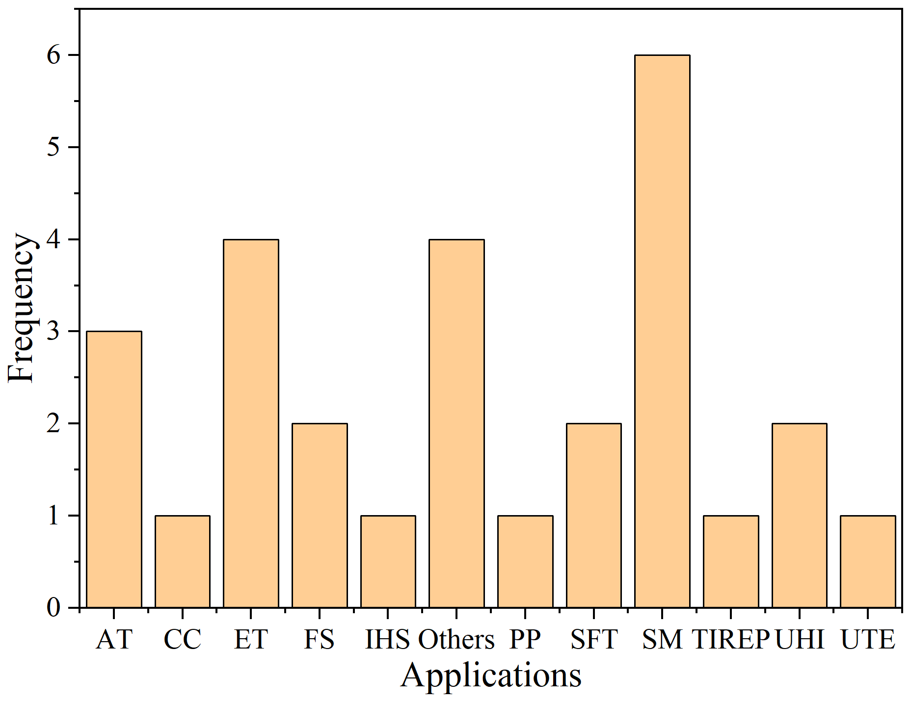
Figure 16Statistics of applications based on TRIMS LST (AT: air temperature; CC: climate change; ET: evapotranspiration; FS: frozen soil; IHS: industrial heat source; others: active layer thickness, lake area, land desertification, and LST downscaling; PP: plant phenology; SFT: soil freeze–thaw; SM: soil moisture; TIREP: thermal infrared earthquake prediction; UHI: urban heat island; UTE: urban thermal environment).
Satellite TIR LSTs are important input data for obtaining SM estimates with high resolution and high spatial coverage. However, most satellite TIR LST products can only be used under clear-sky conditions. The availability of all-sky LST products provides an important opportunity to obtain SMs with spatial seamlessness. Zhang et al. (2023) combined the use of ERA5-Land and TRIMS LST for the fine-scale assessment of soil moisture in China. They used the model based on 0.1∘ ERA5-Land and SM data for 1 km TRIMS LST and finally obtained a daily 1 km SM dataset with satisfactory accuracy. Benefiting from the effective recovery of LST under cloudy conditions, this SM dataset has quasi-full spatial coverage. In addition, Hu et al. (2022) used the TRIMS LST as input data to construct a soil moisture downscaling model for the Tibetan Plateau. The TRIMS LST was found to successfully overcome the challenges of satellite TIR remote sensing detection due to temporal or spatial gaps and false detections due to clouds and topography. Based on the downscaled soil moisture, they further published the daily 0.05∘ × 0.05∘ land surface soil moisture dataset of the Qilian mountain area (northern and northwestern Tibetan Plateau) from 2019 to 2021 (SMHiRes, V2) (Hu et al., 2022; Qu et al., 2021; Chai et al., 2021, 2022a, b).
LST can also be used to investigate the soil freeze–thaw cycles. Li et al. (2023) used the TRIMS LST to obtain thawing degree days and freezing degree days to calculate the soil thermal conductivity and to improve the output of the temperature at the top of the permafrost model. Due to the characteristics of TRIMS LST (high spatial and temporal resolution), the above two metrics can easily be obtained on a spatial scale of 1 km. In addition, the TRIMS LST was also used to evaluate the impact of the LST on the classification accuracy of different remotely sensed or model-based freeze–thaw datasets (Li et al., 2022).
Based on the TRIMS LST, K. Li et al. (2021) investigated the spatial and temporal variations of surface UHI (SUHI) intensity (SUHII). The positive performance of the TRIMS LST in obtaining the LST under cloudy conditions enabled the examination of the SUHII of 305 Chinese cities, especially the cities located in southern China, where clouds frequently appear. Furthermore, Liao et al. (2022) quantified the clear-sky bias of the SUHII by using the MODIS LST based on the TRIMS LST. They emphasized the importance of investigating the SUHI phenomenon under cloudy conditions.
TRIMS LST is available for free and easy access through TPDC at https://doi.org/10.11888/Meteoro.tpdc.271252 (Zhou et al., 2021).
A long-term 1 km daily all-weather LST dataset is the basis for supporting many applications related to land surface processes and climate change. Although some all-weather LST datasets have been released, especially in the last 2 years, users still lack such data for the period of 2000–2002, during which the MODIS LST is not available. In this study, we report a daily 1 km all-weather LST dataset for China's landmass and surrounding areas – TRIMS LST. In contrast to many all-weather LST products, the TRIMS LST begins on the first day of the new millennium (i.e., 1 January 2000).
TRIMS LST is produced based on the E-RTM method. The primary input resources are the Terra/Aqua MODIS LST and GLDAS LST. The TRIMS LST was comprehensively evaluated from four aspects, including comparison with satellite and reanalysis LSTs, validation against the in situ LST, and similarity quantification for the TRIMS-Terra and TRIMS-Aqua LST time series. The results outside the temporal gap period indicate that the TRIMS LST agrees well with the original MODIS and GLDAS LST and the independent ERA5 and AATSR LST but with more spatial details and better spatiotemporal completeness. Validation of TRIMS LST using the in situ LST at 19 ground sites shows that the MBE was −2.26 to 1.73 K and the RMSE was 0.80 to 3.68 K, with slightly better accuracy than the MODIS LST and no obvious difference under different weather conditions. The results within the temporal gap period show that RFSTM and TSETR have similar accuracy performance to the original RTM method, with MBE differences not exceeding 0.40 K and RMSE differences not exceeding 0.7 K. The stability of the TRIMS LST differences for T1 at the Aqua and Terra overpass times is also a side-effect of the excellent quality.
The TRIMS LST has already been released to the scientific community. A series of applications, such as soil moisture estimation and downscaling, surface evapotranspiration estimation, and UHI modeling, has been reported. The TRIMS LST was found to successfully address the cloud contamination of satellite TIR LST with good accuracy, long time series, and spatiotemporal completeness. The TRIMS LST will be continuously updated to satisfy the latest requirements of users.
| Advanced Along-Track Scanning Radiometer | AATSR |
| Advanced Microwave Scanning Radiometer 2 | AMSR2 |
| The Coordinated Energy and Water Cycle Observation Project (CEOP) and the Asia–Australia Monsoon Project (CAMP) | CEOP-CAMP |
| Chinese Ecosystem Research Network | CERN |
| 30 m yearly China land cover dataset (2000–2015) | CLCD |
| Day of the year | DOY |
| Enhanced reanalysis and thermal infrared remote sensing merging method | E-RTM |
| Evapotranspiration | ET |
| Field of view | FOV |
| Goddard Earth Sciences Data and Information Services Center | GES DISC |
| Global Land Data Assimilation System assimilation | GLDAS |
| Global Land Surface Satellite | GLASS |
| HaiHe Experiment in the Hai River Basin, China | HHE |
| Heihe Watershed Allied Telemetry Experimental Research | HiWATER |
| Land surface temperature | LST |
| Mean bias deviation | MBD |
| Mean bias error | MBE |
| MSG All-Sky Land Surface Temperature | MLST-AS |
| Moderate Resolution Imaging Spectroradiometer | MODIS |
| Northwest Institute of Eco-Environment and Resources, Chinese Academy of Sciences | NIEER-CAS |
| Normalized Difference Snow Index | NDSI |
| Normalized Difference Vegetation Index | NDVI |
| Passive microwave | PMW |
| Random-forest-based spatiotemporal merging approach | RFSTM |
| Root mean square error | RMSE |
| Soil moisture | SM |
| Satellite Pour l'Observation de la Terre (SPOT) VEGETATION (VGT) | SPOT VGT |
| Shuttle Radar Topography Mission digital elevation model | SRTM DEM |
| Standard deviation | SD |
| Surface UHI | SUHI |
| Surface UHI intensity | SUHII |
| Thermal infrared | TIR |
| National Tibetan Plateau Data Center | TPDC |
| Thermal and Reanalysis Integrating Moderate-resolution Spatial-seamless LST | TRIMS LST |
| Time series angle | TSA |
| Time-sequential LST-based reconstruction approach | TSETR |
| Urban heat island | UHI |
| Visible Infrared Imaging Radiometer | VIIRS |
Table B1MBE and RMSE from validation results of the daytime TRIMS LST and MODIS LST with in situ LST.
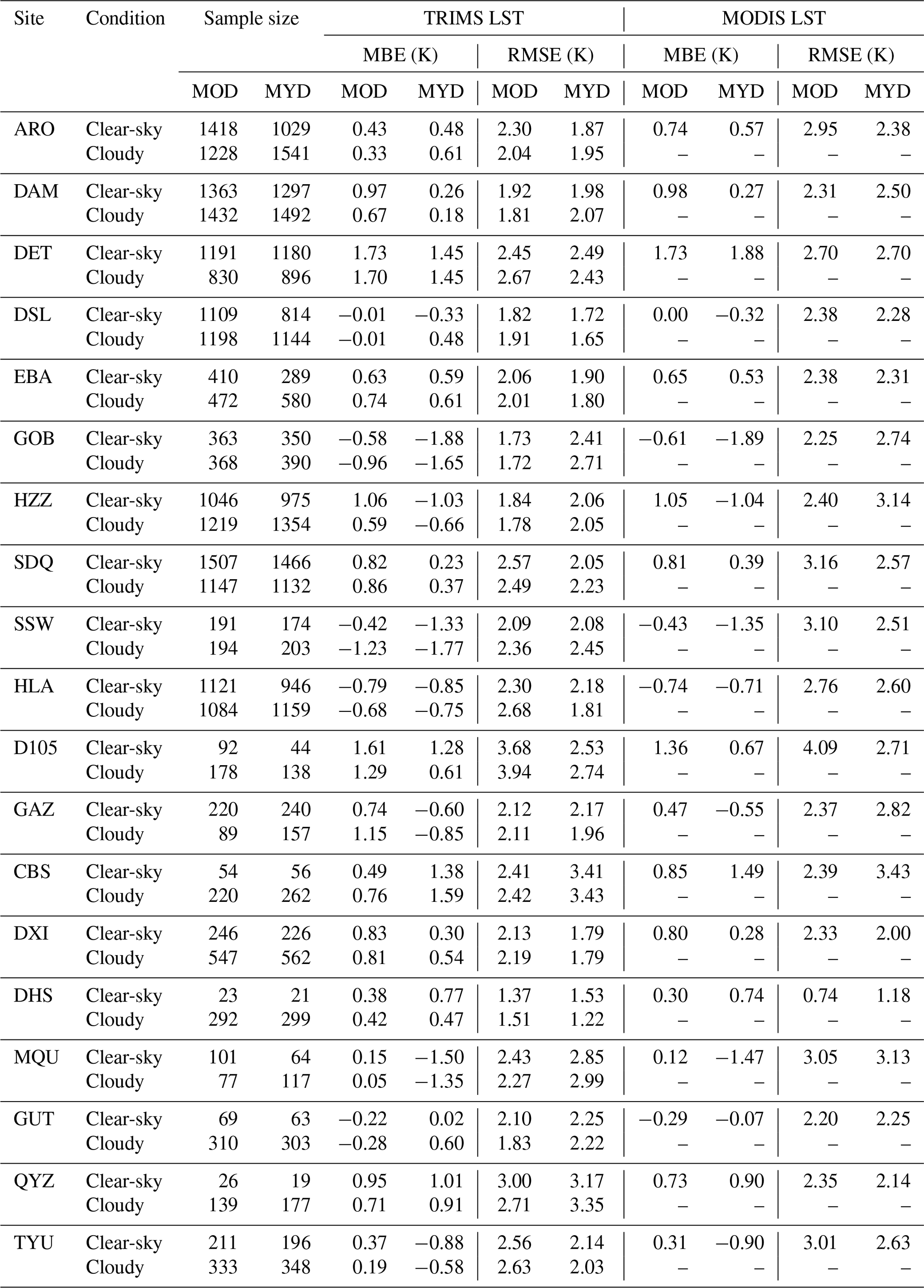
Table B2MBE and RMSE from validation results of the nighttime TRIMS LST and MODIS LST with the in situ LST.
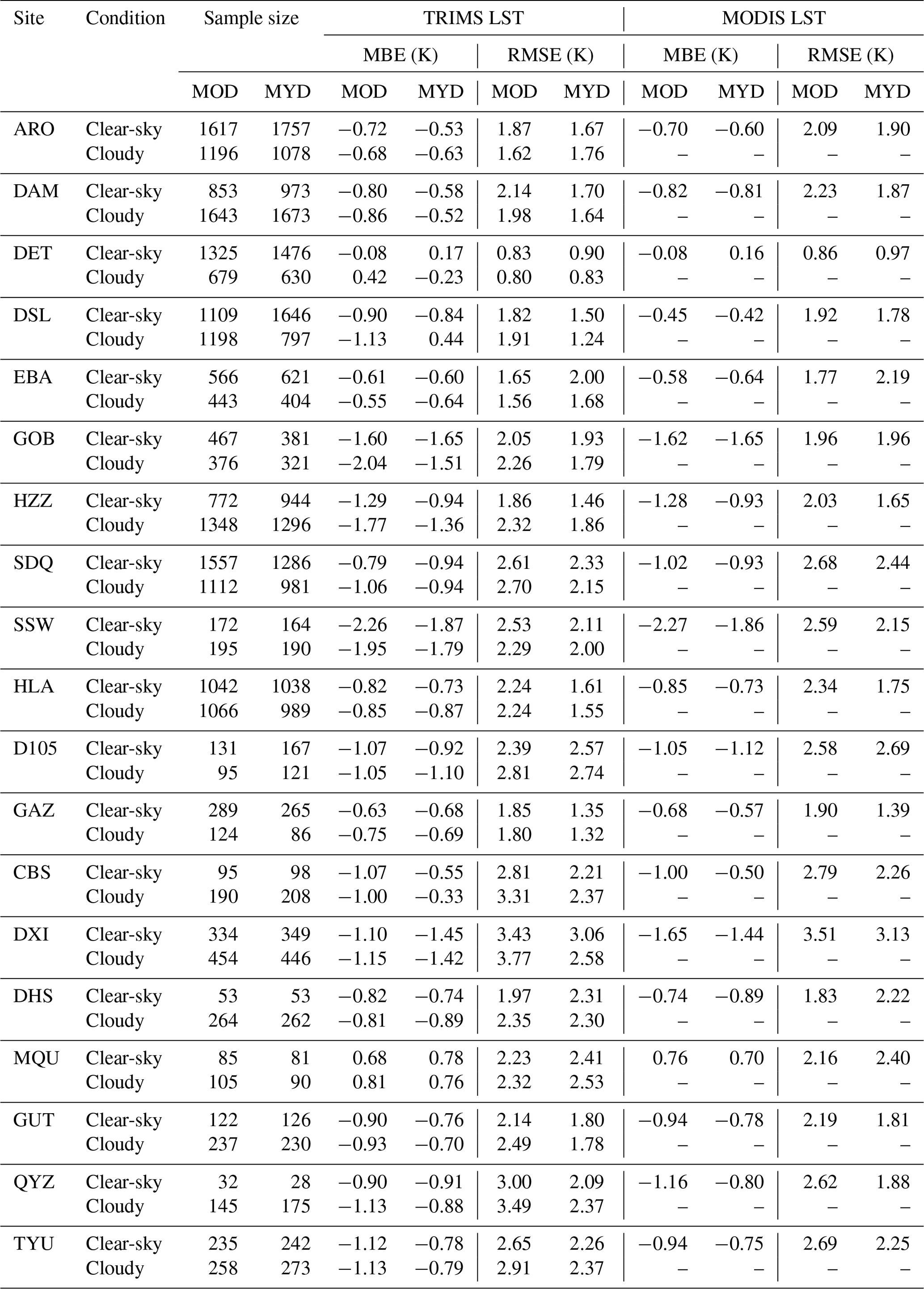
Table C1Summary of publicly available all-weather, all-sky, and gap-free LST products.
WBT implemented the E-RTM method, completed the thorough evaluation, and wrote the earliest version of the manuscript. JZ organized this research, examined the entire process of generation and release of the TRIMS LST dataset, and provided the necessary guidance. JM helped to obtain the measured data and provided the method to quantify the spatial representation. XDZ and JZ proposed the original RTM method. All the co-authors contributed to the writing and carefully reviewed and revised the manuscript.
The contact author has declared that none of the authors has any competing interests.
Publisher's note: Copernicus Publications remains neutral with regard to jurisdictional claims made in the text, published maps, institutional affiliations, or any other geographical representation in this paper. While Copernicus Publications makes every effort to include appropriate place names, the final responsibility lies with the authors.
The authors would like to thank EARTHDATA, the Goddard Earth Sciences Data and Information Services Center, the National Tibetan Plateau Data Center, and the Global Flux Network (http://www.fluxnet.org, last access: 8 January 2024) for providing the MODIS, GLDAS, and ground measurements. We also acknowledge the Centre for Environmental Data Analysis, the European Centre for Medium-Range Weather Forecasts, the CGIAR Consortium for Spatial Information, the Terrascope project, the University of Maryland, and Zenodo for providing the AATSR LST, ERA5-Land LST, SRTM DEM, SPOT VGT, GLASS albedo product, and 30 m yearly China land cover dataset (2000–2015).
This study was supported by the National Natural Science Foundation of China under grant nos. 42271387 and 42201417, the Science Fund for Distinguished Young Scholars of Sichuan Province under grant no. 2023NSFSC1907, the Fundamental Research Funds for the Central Universities of China, University of Electronic Science and Technology of China under grant no. ZYGX2019J069, and the China Scholarship Council under grant no. 202306070058.
This paper was edited by Di Tian and reviewed by Aolin Jia and two anonymous referees.
Aguilar-Lome, J., Espinoza-Villar, R., Espinoza, J.-C., Rojas-Acuna, J., Leo Willems, B., and Leyva-Molina, W.-M.: Elevation-dependent warming of land surface temperatures in the Andes assessed using MODIS LST time series (2000–2017), Int. J. Appl. Earth Obs., 77, 119–128, https://doi.org/10.1016/j.jag.2018.12.013, 2019.
Alexander, C.: Normalised difference spectral indices and urban land cover as indicators of land surface temperature (LST), Int. J. Appl. Earth Obs., 86, 102013, https://doi.org/10.1016/j.jag.2019.102013, 2020.
Anderson, M. C., Kustas, W. P., Norman, J. M., Hain, C. R., Mecikalski, J. R., Schultz, L., González-Dugo, M. P., Cammalleri, C., d'Urso, G., Pimstein, A., and Gao, F.: Mapping daily evapotranspiration at field to continental scales using geostationary and polar orbiting satellite imagery, Hydrol. Earth Syst. Sci., 15, 223–239, https://doi.org/10.5194/hess-15-223-2011, 2011.
Bechtel, B.: A New Global Climatology of Annual Land Surface Temperature, Remote Sens.-Basel, 7, 2850–2870, https://doi.org/10.3390/rs70302850, 2015.
Breiman, L.: Random Forests, Mach. Learn., 45, 5–32, https://doi.org/10.1023/A:1010933404324, 2001.
Chai, L., Zhu, Z., and Liu, S.: Daily land surface soil moisture dataset of Qilian Mountain area (2019,SMHiRes,V2), National Tibetan Plateau/Third Pole Environment Data Center [data set], https://doi.org/10.11888/Terre.tpdc.300976, 2021.
Chai, L., Zhu, Z., and Liu, S.: Daily land surface soil moisture dataset of Qilian Mountain area (2020,SMHiRes,V2), National Tibetan Plateau/Third Pole Environment Data Center [data set], https://doi.org/10.11888/Terre.tpdc.272375, 2022a.
Chai, L., Zhu, Z., and Liu, S.: Daily land surface soil moisture dataset of Qilian Mountain area (2021,SMHiRes,V2), National Tibetan Plateau/Third Pole Environment Data Center [data set], https://doi.org/10.11888/Terre.tpdc.272376, 2022b.
Che, T., Li, X., Liu, S., Li, H., Xu, Z., Tan, J., Zhang, Y., Ren, Z., Xiao, L., Deng, J., Jin, R., Ma, M., Wang, J., and Yang, X.: Integrated hydrometeorological, snow and frozen-ground observations in the alpine region of the Heihe River Basin, China, Earth Syst. Sci. Data, 11, 1483–1499, https://doi.org/10.5194/essd-11-1483-2019, 2019.
Chen, A., Meng, W., Hu, S., and Bian, A.: Comparative analysis on land surface albedo from MODIS and GLASS over the Tibetan Plateau, Trans. Atmos. Sci., 43, 932–942, https://doi.org/10.13878/j.cnki.dqkxxb.20171030001, 2020.
Chen, C., Park, T., Wang, X., Piao, S., Xu, B., Chaturvedi, R. K., Fuchs, R., Brovkin, V., Ciais, P., Fensholt, R., Tømmervik, H., Bala, G., Zhu, Z., Nemani, R. R., and Myneni, R. B.: China and India lead in greening of the world through land-use management, Nat. Sustain., 2, 122–129, https://doi.org/10.1038/s41893-019-0220-7, 2019.
Chen, S., Chen, X., Chen, W., Su, Y., and Li, D.: A simple retrieval method of land surface temperature from AMSR-E passive microwave data—A case study over Southern China during the strong snow disaster of 2008, Int. J. Appl. Earth Obs., 13, 140–151, 2011.
Chen, Y., Chen, W., Su, Q., Luo, F., Sparrow, S., Wallom, D., Tian, F., Dong, B., Tett, S. F. B., and Lott, F. C.: Anthropogenic Warming has Substantially Increased the Likelihood of July 2017–Like Heat Waves over Central Eastern China, B. Am. Meteorol. Soc., 100, S91–S95, https://doi.org/10.1175/BAMS-D-18-0087.1, 2019.
Coops, N. C., Duro, D. C., Wulder, M. A., and Han, T.: Estimating afternoon MODIS land surface temperatures (LST) based on morning MODIS overpass, location and elevation information, Int. J. Remote Sens., 28, 2391–2396, https://doi.org/10.1080/01431160701294653, 2007.
Ding, L., Zhou, J., Li, Z.-L., Ma, J., Shi, C., Sun, S., and Wang, Z.: Reconstruction of Hourly All-Weather Land Surface Temperature by Integrating Reanalysis Data and Thermal Infrared Data From Geostationary Satellites (RTG), IEEE T. Geosci. Remote, 60, 1–17, https://doi.org/10.1109/TGRS.2022.3227074, 2022.
Ding, L., Zhou, J., Zhang, X., Wang, S., Tang, W., Wang, Z., Ma, J., Ai, L., Li, M., and Wang, W.: Estimation of all-weather land surface temperature with remote sensing: Progress and challenges, National Remote Sensing Bulletin, 27, 1534–1553, https://doi.org/10.11834/jrs.20211323, 2023.
Dong, S., Cheng, J., Shi, J., Shi, C., Sun, S., and Liu, W.: A Data Fusion Method for Generating Hourly Seamless Land Surface Temperature from Himawari-8 AHI Data, Remote Sens.-Basel, 14, 5170, https://doi.org/10.3390/rs14205170, 2022.
Duan, S., Li, Z., and Leng, P.: A framework for the retrieval of all-weather land surface temperature at a high spatial resolution from polar-orbiting thermal infrared and passive microwave data, Remote Sens. Environ., 195, 107–117, https://doi.org/10.1016/j.rse.2017.04.008, 2017.
Duan, S.-B., Li, Z.-L., Li, H., Göttsche, F.-M., Wu, H., Zhao, W., Leng, P., Zhang, X., and Coll, C.: Validation of Collection 6 MODIS land surface temperature product using in situ measurements, Remote Sens. Environ., 225, 16–29, https://doi.org/10.1016/j.rse.2019.02.020, 2019.
Feng, Y., Liu, Q., Qu, Y., and Liang, S.: Estimation of the Ocean Water Albedo From Remote Sensing and Meteorological Reanalysis Data, IEEE T. Geosci. Remote, 54, 850–868, https://doi.org/10.1109/TGRS.2015.2468054, 2016.
Freitas, S. C., Trigo, I. F., Bioucas-Dias, J. M., and Gottsche, F.-M.: Quantifying the Uncertainty of Land Surface Temperature Retrievals From SEVIRI/Meteosat, IEEE T. Geosci. Remote, 48, 523–534, https://doi.org/10.1109/TGRS.2009.2027697, 2010.
Fu, B., Li, S., Yu, X., Yang, P., Yu, G., Feng, R., and Zhuang, X.: Chinese ecosystem research network: Progress and perspectives, Ecol. Complex., 7, 225–233, https://doi.org/10.1016/j.ecocom.2010.02.007, 2010.
Göttsche, F.-M., Olesen, F.-S., Trigo, I. F., Bork-Unkelbach, A., and Martin, M. A.: Long Term Validation of Land Surface Temperature Retrieved from MSG/SEVIRI with Continuous in-Situ Measurements in Africa, Remote Sens.-Basel, 8, 410, https://doi.org/10.3390/rs8050410, 2016.
Guo, A., Liu, S., Zhu, Z., Xu, Z., Xiao, Q., Ju, Q., Zhang, Y., and Yang, X.: Impact of Lake/Reservoir Expansion and Shrinkage on Energy and Water Vapor Fluxes in the Surrounding Area, J. Geophys. Res.-Atmos., 125, e2020JD032833, https://doi.org/10.1029/2020JD032833, 2020.
He, T., Liang, S., and Song, D.-X.: Analysis of global land surface albedo climatology and spatial-temporal variation during 1981–2010 from multiple satellite products, J. Geophys. Res.-Atmos., 119, 10281–10-298, https://doi.org/10.1002/2014JD021667, 2014.
Holmes, T. R. H., De Jeu, R. A. M., Owe, M., and Dolman, A. J.: Land surface temperature from Ka band (37 GHz) passive microwave observations, J. Geophys. Res.-Atmos., 114, https://doi.org/10.1029/2008JD010257, 2009.
Hong, F., Zhan, W., Göttsche, F.-M., Liu, Z., Dong, P., Fu, H., Huang, F., and Zhang, X.: A global dataset of spatiotemporally seamless daily mean land surface temperatures: generation, validation, and analysis, Earth Syst. Sci. Data, 14, 3091–3113, https://doi.org/10.5194/essd-14-3091-2022, 2022a.
Hong, F., Zhan, W., Göttsche, F., Liu, Z., Dong, P., Fu, H., Huang, F., and Zhang, X.: A global spatiotemporally seamless daily mean land surface temperature from 2003 to 2019 (v1.0), Zenodo [data set], https://doi.org/10.5281/zenodo.6287052, 2022b.
Hu, Z., Chai, L., Crow, W. T., Liu, S., Zhu, Z., Zhou, J., Qu, Y., Liu, J., Yang, S., and Lu, Z.: Applying a Wavelet Transform Technique to Optimize General Fitting Models for SM Analysis: A Case Study in Downscaling over the Qinghai-Tibet Plateau, Remote Sens.-Basel, 14, 3063, https://doi.org/10.3390/rs14133063, 2022.
Jia, A., Ma, H., Liang, S., and Wang, D.: Cloudy-sky land surface temperature from VIIRS and MODIS satellite data using a surface energy balance-based method, Remote Sens. Environ., 263, 112566, https://doi.org/10.1016/j.rse.2021.112566, 2021.
Jia, A., Liang, S., and Wang, D.: Generating a 2-km, all-sky, hourly land surface temperature product from Advanced Baseline Imager data, Remote Sens. Environ., 278, 113105, https://doi.org/10.1016/j.rse.2022.113105, 2022a.
Jia, A., Liang, S., Wang, D., Ma, L., Wang, Z., and Xu, S.: Global Hourly, 5-km, All-sky Land Surface Temperature (GHA-LST), In Earth System Science Data (ESSD): Bd. x (Version 01, Nummer x, S. x), Zenodo [data set], https://doi.org/10.5281/zenodo.6981704, 2022b.
Jia, A., Liang, S., Wang, D., Ma, L., Wang, Z., and Xu, S.: Global hourly, 5 km, all-sky land surface temperature data from 2011 to 2021 based on integrating geostationary and polar-orbiting satellite data, Earth Syst. Sci. Data, 15, 869–895, https://doi.org/10.5194/essd-15-869-2023, 2023.
Jiang, G.-M. and Liu, R.: Retrieval of Sea and Land Surface Temperature From SVISSR/FY-2C/D/E Measurements, IEEE T. Geosci. Remote, 52, 6132–6140, https://doi.org/10.1109/TGRS.2013.2295260, 2014.
Jin, M. and Dickinson, R. E.: A generalized algorithm for retrieving cloudy sky skin temperature from satellite thermal infrared radiances, J. Geophys. Res.-Atmos., 105, 27037–27047, https://doi.org/10.1029/2000JD900318, 2000.
Kruse, F., Lefkoff, A., Boardman, J., Heidebrecht, K., Shapiro, A., Barloon, P., and Goetz, A.: The Spectral Image-Processing System (sips) - Interactive Visualization and Analysis of Imaging Spectrometer Data, Remote Sens. Environ., 44, 145–163, https://doi.org/10.1016/0034-4257(93)90013-N, 1993.
Li, B., Liang, S., Liu, X., Ma, H., Chen, Y., Liang, T., and He, T.: Estimation of all-sky 1 km land surface temperature over the conterminous United States, Remote Sens. Environ., 266, 112707, https://doi.org/10.1016/j.rse.2021.112707, 2021.
Li, H., Liu, Q., Yang, Y., Li, R., Wang, H., Cao, B., Bian, Z., Hu, T., Du, Y., and Sun, L.: Comparison of the MuSyQ and MODIS Collection 6 Land Surface Temperature Products Over Barren Surfaces in the Heihe River Basin, China, IEEE T. Geosci. Remote, 57, 8081–8094, https://doi.org/10.1109/TGRS.2019.2918259, 2019.
Li, H., Chai, L., Crow, W., Dong, J., Liu, S., and Zhao, S.: The reliability of categorical triple collocation for evaluating soil freeze/ thaw datasets, Remote Sens. Environ., 281, https://doi.org/10.1016/j.rse.2022.113240, 2022.
Li, K., Chen, Y., and Gao, S.: Comparative Analysis of Variations and Patterns between Surface Urban Heat Island Intensity and Frequency across 305 Chinese Cities, Remote Sens.-Basel, 13, 3505, https://doi.org/10.3390/rs13173505, 2021.
Li, W., Weng, B., Yan, D., Lai, Y., Li, M., and Wang, H.: Underestimated permafrost degradation: Improving the TTOP model based on soil thermal conductivity, Sci. Total Environ., 854, https://doi.org/10.1016/j.scitotenv.2022.158564, 2023.
Li, X., Cheng, G., Liu, S., Xiao, Q., Ma, M., Jin, R., Che, T., Liu, Q., Wang, W., Qi, Y., Wen, J., Li, H., Zhu, G., Guo, J., Ran, Y., Wang, S., Zhu, Z., Zhou, J., Hu, X., and Xu, Z.: Heihe Watershed Allied Telemetry Experimental Research (HiWATER): Scientific Objectives and Experimental Design, B. Am. Meteorol. Soc., 94, 1145–1160, https://doi.org/10.1175/BAMS-D-12-00154.1, 2013.
Li, X., Zhou, Y., Asrar, G. R., and Zhu, Z.: Creating a seamless 1km resolution daily land surface temperature dataset for urban and surrounding areas in the conterminous United States, Remote Sens. Environ., 206, 84–97, https://doi.org/10.1016/j.rse.2017.12.010, 2018.
Li, Y., Li, Z.-L., Wu, H., Zhou, C., Liu, X., Leng, P., Yang, P., Wu, W., Tang, R., Shang, G.-F., and Ma, L.: Biophysical impacts of earth greening can substantially mitigate regional land surface temperature warming, Nat. Commun., 14, 121, https://doi.org/10.1038/s41467-023-35799-4, 2023b.
Li, Z.-L., Tang, B.-H., Wu, H., Ren, H., Yan, G., Wan, Z., Trigo, I. F., and Sobrino, J. A.: Satellite-derived land surface temperature: Current status and perspectives, Remote Sens. Environ., 131, 14–37, https://doi.org/10.1016/j.rse.2012.12.008, 2013.
Li, Z.-L., Wu, H., Duan, S.-B., Zhao, W., Ren, H., Liu, X., Leng, P., Tang, R., Ye, X., Zhu, J., Sun, Y., Si, M., Liu, M., Li, J., Zhang, X., Shang, G., Tang, B.-H., Yan, G., and Zhou, C.: Satellite Remote Sensing of Global Land Surface Temperature: Definition, Methods, Products, and Applications, Rev. Geophys., 61, e2022RG000777, https://doi.org/10.1029/2022RG000777, 2023.
Liao, Y., Shen, X., Zhou, J., Ma, J., Zhang, X., Tang, W., Chen, Y., Ding, L., and Wang, Z.: Surface urban heat island detected by all-weather satellite land surface temperature, Sci. Total Environ., 811, 151405, https://doi.org/10.1016/j.scitotenv.2021.151405, 2022.
Liu, H., Dong, W., Fu, C., and Shi, L.: The Long-Term Field Experiment on Aridification and the Ordered Human Activity in Semi-Arid Area at Tongyu, Northeast China, Climatic and Environmental Research, 9, 378–389, https://doi.org/10.3878/j.issn.1006-9585.2004.02.14, 2004.
Liu, N. F., Liu, Q., Wang, L. Z., Liang, S. L., Wen, J. G., Qu, Y., and Liu, S. H.: A statistics-based temporal filter algorithm to map spatiotemporally continuous shortwave albedo from MODIS data, Hydrol. Earth Syst. Sci., 17, 2121–2129, https://doi.org/10.5194/hess-17-2121-2013, 2013.
Liu, S., Li, X., Xu, Z., Che, T., Xiao, Q., Ma, M., Liu, Q., Jin, R., Guo, J., Wang, L., Wang, W., Qi, Y., Li, H., Xu, T., Ran, Y., Hu, X., Shi, S., Zhu, Z., Tan, J., Zhang, Y., and Ren, Z.: The Heihe Integrated Observatory Network: A Basin-Scale Land Surface Processes Observatory in China, Vadose Zone J., 17, 180072, https://doi.org/10.2136/vzj2018.04.0072, 2018.
Liu, S. M., Xu, Z. W., Wang, W. Z., Jia, Z. Z., Zhu, M. J., Bai, J., and Wang, J. M.: A comparison of eddy-covariance and large aperture scintillometer measurements with respect to the energy balance closure problem, Hydrol. Earth Syst. Sci., 15, 1291–1306, https://doi.org/10.5194/hess-15-1291-2011, 2011.
Liu, S. M., Xu, Z. W., Zhu, Z. L., Jia, Z. Z., and Zhu, M. J.: Measurements of evapotranspiration from eddy-covariance systems and large aperture scintillometers in the Hai River Basin, China, J. Hydrol., 487, 24–38, https://doi.org/10.1016/j.jhydrol.2013.02.025, 2013.
Liu, S., Xu, Z., Che, T., Li, X., Xu, T., Ren, Z., Zhang, Y., Tan, J., Song, L., Zhou, J., Zhu, Z., Yang, X., Liu, R., and Ma, Y.: A dataset of energy, water vapor, and carbon exchange observations in oasis–desert areas from 2012 to 2021 in a typical endorheic basin, Earth Syst. Sci. Data, 15, 4959–4981, https://doi.org/10.5194/essd-15-4959-2023, 2023.
Liu, Y., Hiyama, T., and Yamaguchi, Y.: Scaling of land surface temperature using satellite data: A case examination on ASTER and MODIS products over a heterogeneous terrain area, Remote Sens. Environ., 105, 115–128, https://doi.org/10.1016/j.rse.2006.06.012, 2006.
Long, D., Yan, L., Bai, L., Zhang, C., Li, X., Lei, H., Yang, H., Tian, F., Zeng, C., Meng, X., and Shi, C.: Generation of MODIS-like land surface temperatures under all-weather conditions based on a data fusion approach, Remote Sens. Environ., 246, 111863, https://doi.org/10.1016/j.rse.2020.111863, 2020.
Lu, Y., Wang, L., Hu, B., Zhang, M., Qin, W., Zhou, J., and Tao, M.: Evaluation of satellite land surface albedo products over China using ground-measurements, Int. J. Digit. Earth, 14, 1493–1513, https://doi.org/10.1080/17538947.2021.1946179, 2021.
Ma, J., Zhou, J., Liu, S., Göttsche, F.-M., Zhang, X., Wang, S., and Li, M.: Continuous evaluation of the spatial representativeness of land surface temperature validation sites, Remote Sens. Environ., 265, 112669, https://doi.org/10.1016/j.rse.2021.112669, 2021.
Ma, J., Zhou, J., Göttsche, F.-M., Wang, Z., Wu, H., Tang, W., Li, M., and Liu, S.: An atmospheric influence correction method for longwave radiation-based in-situ land surface temperature, Remote Sens. Environ., 293, 113611, https://doi.org/10.1016/j.rse.2023.113611, 2023.
Ma, Y., Yao, T., and Wang, J.: Experimental study of energy and water cycle in Tibetan Plateau: The progress introduction on the study of GAME/Tibet and CAMP/Tibet, Plateau Meteorol., 25, 344–351, 2006.
Ma, Y., Zhou, J., Liu, S., Zhang, W., Zhang, Y., Xu, Z., Song, L., and Zhao, H.: Estimation of evapotranspiration using all-weather land surface temperature and variational trends with warming temperatures for the River Source Region in Southwest China, J. Hydrol., 613, 128346, https://doi.org/10.1016/j.jhydrol.2022.128346, 2022.
Martins, J. P. A., Trigo, I. F., Ghilain, N., Jimenez, C., Göttsche, F.-M., Ermida, S. L., Olesen, F.-S., Gellens-Meulenberghs, F., and Arboleda, A.: An All-Weather Land Surface Temperature Product Based on MSG/SEVIRI Observations, Remote Sens.-Basel, 11, 3044, https://doi.org/10.3390/rs11243044, 2019.
Meng, Y., Zhou, J., Göttsche, F.-M., Tang, W., Martins, J., Perez-Planells, L., Ma, J., and Wang, Z.: Investigation and validation of two all-weather land surface temperature products with in-situ measurements, Geo-spatial Information Science, 1–13, https://doi.org/10.1080/10095020.2023.2255037, 2023.
Metz, M., Andreo, V., and Neteler, M.: A New Fully Gap-Free Time Series of Land Surface Temperature from MODIS LST Data, Remote Sens.-Basel, 9, 1333, https://doi.org/10.3390/rs9121333, 2017a.
Metz, M., Andreo, V., and Neteler, M.: Monthly MODIS LST data related to the article: A new fully gap-free time series of land surface temperature from MODIS LST data, In Remote Sensing (1.0.0, Bd. 9, Nummer 12, S. 1333), Zenodo [data set], https://doi.org/10.5281/zenodo.1115666, 2017b.
Mildrexler, D. J., Zhao, M., Cohen, W. B., Running, S. W., Song, X. P., and Jones, M. O.: Thermal Anomalies Detect Critical Global Land Surface Changes, J. Appl. Meteorol. Clim., 57, 391–411, 2018.
Muñoz-Sabater, J., Dutra, E., Agustí-Panareda, A., Albergel, C., Arduini, G., Balsamo, G., Boussetta, S., Choulga, M., Harrigan, S., Hersbach, H., Martens, B., Miralles, D. G., Piles, M., Rodríguez-Fernández, N. J., Zsoter, E., Buontempo, C., and Thépaut, J.-N.: ERA5-Land: a state-of-the-art global reanalysis dataset for land applications, Earth Syst. Sci. Data, 13, 4349–4383, https://doi.org/10.5194/essd-13-4349-2021, 2021.
Parinussa, R., Lakshmi, V., Johnson, F., and Sharma, A.: Comparing and Combining Remotely Sensed Land Surface Temperature Products for Improved Hydrological Applications, Remote Sens.-Basel, 8, 162, https://doi.org/10.3390/rs8020162, 2016.
Pastorello, G., Trotta, C., Canfora, E., Chu, H., Christianson, D., Cheah, Y.-W., Poindexter, C., Chen, J., Elbashandy, A., Humphrey, M., Isaac, P., Polidori, D., Reichstein, M., Ribeca, A., van Ingen, C., Vuichard, N., Zhang, L., Amiro, B., Ammann, C., Arain, M. A., Ardö, J., Arkebauer, T., Arndt, S. K., Arriga, N., Aubinet, M., Aurela, M., Baldocchi, D., Barr, A., Beamesderfer, E., Marchesini, L. B., Bergeron, O., Beringer, J., Bernhofer, C., Berveiller, D., Billesbach, D., Black, T. A., Blanken, P. D., Bohrer, G., Boike, J., Bolstad, P. V., Bonal, D., Bonnefond, J.-M., Bowling, D. R., Bracho, R., Brodeur, J., Brümmer, C., Buchmann, N., Burban, B., Burns, S. P., Buysse, P., Cale, P., Cavagna, M., Cellier, P., Chen, S., Chini, I., Christensen, T. R., Cleverly, J., Collalti, A., Consalvo, C., Cook, B. D., Cook, D., Coursolle, C., Cremonese, E., Curtis, P. S., D'Andrea, E., da Rocha, H., Dai, X., Davis, K. J., Cinti, B. D., Grandcourt, A. de, Ligne, A. D., De Oliveira, R. C., Delpierre, N., Desai, A. R., Di Bella, C. M., Tommasi, P. di, Dolman, H., Domingo, F., Dong, G., Dore, S., Duce, P., Dufrêne, E., Dunn, A., Dušek, J., Eamus, D., Eichelmann, U., ElKhidir, H. A. M., Eugster, W., Ewenz, C. M., Ewers, B., Famulari, D., Fares, S., Feigenwinter, I., Feitz, A., Fensholt, R., Filippa, G., Fischer, M., Frank, J., Galvagno, M., et al.: The FLUXNET2015 dataset and the ONEFlux processing pipeline for eddy covariance data, Sci. Data, 7, 225, https://doi.org/10.1038/s41597-020-0534-3, 2020.
Peng, S.-S., Piao, S., Zeng, Z., Ciais, P., Zhou, L., Li, L. Z. X., Myneni, R. B., Yin, Y., and Zeng, H.: Afforestation in China cools local land surface temperature, P. Natl. Acad. Sci. USA, 111, 2915–2919, https://doi.org/10.1073/pnas.1315126111, 2014.
Qu, Y., Zhu, Z., Montzka, C., Chai, L., Liu, S., Ge, Y., Liu, J., Lu, Z., He, X., Zheng, J., and Han, T.: Inter-comparison of several soil moisture downscaling methods over the Qinghai-Tibet Plateau, China, J. Hydrol., 592, 125616, https://doi.org/10.1016/j.jhydrol.2020.125616, 2021.
Quan, J., Guan, Y., Zhan, W., Ma, T., Wang, D., and Guo, Z.: Generating 60–100 m, hourly, all-weather land surface temperatures based on the Landsat, ECOSTRESS, and reanalysis temperature combination (LERC), ISPRS J. Photogram., 205, 115–134, https://doi.org/10.1016/j.isprsjprs.2023.10.004, 2023.
Radakovich, J., Houser, P., Da Silva, A., and Bosilovich, M.: Results From Global Land-surface Data Assimilation Methods, AGU Spring Meeting Abstracts, 1, 2001.
Rains, D.: LSTRAD (0.31), Zenodo [data set], https://doi.org/10.5281/zenodo.7026612, 2022.
Rains, D., Trigo, I., Dutra, E., Ermida, S., Ghent, D., Hulsman, P., Gómez-Dans, J., and Miralles, D. G.: High-resolution all-sky land surface temperature and net radiation over Europe, Earth Syst. Sci. Data Discuss. [preprint], https://doi.org/10.5194/essd-2022-302, in review, 2022.
Rodell, M., Houser, P. R., Jambor, U., Gottschalck, J., Mitchell, K., Meng, C.-J., Arsenault, K., Cosgrove, B., Radakovich, J., Bosilovich, M., Entin, J. K., Walker, J. P., Lohmann, D., and Toll, D.: The Global Land Data Assimilation System, B. Am. Meteorol. Soc., 85, 381–394, https://doi.org/10.1175/BAMS-85-3-381, 2004.
Sandeep, P., Reddy, G. P. O., Jegankumar, R., and Kumar, K. C. A.: Monitoring of agricultural drought in semi-arid ecosystem of Peninsular India through indices derived from time-series CHIRPS and MODIS datasets, Ecol. Indic., 121, 107033, https://doi.org/10.1016/j.ecolind.2020.107033, 2021.
Shiff, S., Helman, D., and Lensky, I. M.: Worldwide continuous gap-filled MODIS land surface temperature dataset, Sci. Data, 8, 74, https://doi.org/10.1038/s41597-021-00861-7, 2021.
Sims, D. A., Rahman, A. F., Cordova, V. D., El-Masri, B. Z., Baldocchi, D. D., Bolstad, P. V., Flanagan, L. B., Goldstein, A. H., Hollinger, D. Y., Misson, L., Monson, R. K., Oechel, W. C., Schmid, H. P., Wofsy, S. C., and Xu, L.: A new model of gross primary productivity for North American ecosystems based solely on the enhanced vegetation index and land surface temperature from MODIS, Remote Sens. Environ., 112, 1633–1646, https://doi.org/10.1016/j.rse.2007.08.004, 2008.
Sobrino, J. A., Jimenez-Munoz, J. C., and Paolini, L.: Land surface temperature retrieval from LANDSAT TM 5, Remote Sens. Environ., 90, 434–440, https://doi.org/10.1016/j.rse.2004.02.003, 2004.
Toté, C., Swinnen, E., Sterckx, S., Clarijs, D., Quang, C., and Maes, R.: Evaluation of the SPOT/VEGETATION Collection 3 reprocessed dataset: Surface reflectances and NDVI, Remote Sens. Environ., 201, 219–233, https://doi.org/10.1016/j.rse.2017.09.010, 2017.
U.S. Geological Survey: Landsat 8 Collection2 (C2) Level 2 Science Product (L2SP) Guide. Nasa, 3 (September), https://d9-wret.s3.us-west-2.amazonaws.com/assets/palladium/production/s3fs-public/media/files/LSDS-1619_Landsat8-9-Collection2-Level2-Science-Product-Guide-v5.pdf (last access: 8 January 2024), 2021.
Wan, Z.: New refinements and validation of the collection-6 MODIS land-surface temperature/emissivity product, Remote Sens. Environ., 140, 36–45, https://doi.org/10.1016/j.rse.2013.08.027, 2014.
Wang, B., Gao, P., Niu, X., and Sun, J.: Policy-driven China's Grain to Green Program: Implications for ecosystem services, Ecosyst. Serv., 27, 38–47, https://doi.org/10.1016/j.ecoser.2017.07.014, 2017.
Wang, L., Zheng, X., Sun, L., Liu, Q., and Liu, S.: Validation of GLASS albedo product through Landsat TM data and ground measurements, J. Remote Sens., 18, 547–558, https://doi.org/10.11834/jrs.20143130, 2014.
Wang, S., Zhou, J., Lei, T., Wu, H., Zhang, X., Ma, J., and Zhong, H.: Estimating Land Surface Temperature from Satellite Passive Microwave Observations with the Traditional Neural Network, Deep Belief Network, and Convolutional Neural Network, Remote Sens.-Basel, 12, 2691, https://doi.org/10.3390/rs12172691, 2020.
Wen, J., Lan, Y., Su, Z., Tian, H., Shi, X., Zhang, Y., Wang, X., Liu, R., Zhang, T., Kang, Y., Lv, S., and Zhang, J.: Advances in observation and modeling of land surface processes over the source region of the Yellow River, Adv. Earth Sci., 26, 575–585, 2011.
Weng, Q. and Fu, P.: Modeling annual parameters of clear-sky land surface temperature variations and evaluating the impact of cloud cover using time series of Landsat TIR data, Remote Sens. Environ., 140, 267–278, https://doi.org/10.1016/j.rse.2013.09.002, 2014.
Wu, P., Shen, H., Zhang, L., and Göttsche, F.-M.: Integrated fusion of multi-scale polar-orbiting and geostationary satellite observations for the mapping of high spatial and temporal resolution land surface temperature, Remote Sens. Environ., 156, 169–181, https://doi.org/10.1016/j.rse.2014.09.013, 2015.
Xiao, Y., Zhao, W., Ma, M., Yu, W., Fan, L., Huang, Y., Sun, X., and Lang, Q.: An Integrated Method for the Generation of Spatio-Temporally Continuous LST Product With MODIS/Terra Observations, IEEE T. Geosci. Remote, 61, 1–14, https://doi.org/10.1109/TGRS.2023.3254598, 2023.
Xu, S. and Cheng, J.: A new land surface temperature fusion strategy based on cumulative distribution function matching and multiresolution Kalman filtering, Remote Sens. Environ., 254, 112256, https://doi.org/10.1016/j.rse.2020.112256, 2021.
Xu, S., Cheng, J., and Zhang, Q.: A Random Forest-Based Data Fusion Method for Obtaining All-Weather Land Surface Temperature with High Spatial Resolution, Remote Sens.-Basel, 13, 2211, https://doi.org/10.3390/rs13112211, 2021.
Xu, Z., Liu, S., Li, X., Shi, S., Wang, J., Zhu, Z., Xu, T., Wang, W., and Ma, M.: Intercomparison of surface energy flux measurement systems used during the HiWATER-MUSOEXE, J. Geophys. Res.-Atmos., 118, 13140–13157, https://doi.org/10.1002/2013JD020260, 2013.
Yang, J. and Huang, X.: The 30 m annual land cover dataset and its dynamics in China from 1990 to 2019, Earth Syst. Sci. Data, 13, 3907–3925, https://doi.org/10.5194/essd-13-3907-2021, 2021.
Yang, J., Zhou, J., Göttsche, F.-M., Long, Z., Ma, J., and Luo, R.: Investigation and validation of algorithms for estimating land surface temperature from Sentinel-3 SLSTR data, Int. J. Appl. Earth Obs., 91, 102136, https://doi.org/10.1016/j.jag.2020.102136, 2020.
Yang, N., Shi, H., Tang, H., and Yang, X.: Geographical and temporal encoding for improving the estimation of PM2.5 concentrations in China using end-to-end gradient boosting, Remote Sens. Environ., 269, 112828, https://doi.org/10.1016/j.rse.2021.112828, 2022.
Yao, R., Wang, L., Huang, X., Cao, Q., Wei, J., He, P., Wang, S., and Wang, L.: Global seamless and high-resolution temperature dataset (GSHTD), 2001–2020, Remote Sens. Environ., 286, 113422, https://doi.org/10.1016/j.rse.2022.113422, 2023.
Yoo, C., Im, J., Cho, D., Yokoya, N., Xia, J., and Bechtel, B.: Estimation of All-Weather 1 km MODIS Land Surface Temperature for Humid Summer Days, Remote Sens.-Basel, 12, 1398, https://doi.org/10.3390/rs12091398, 2020.
Yu, G., Zhang, L., and Sun, X.: Progresses and prospects of Chinese terrestrial ecosystem flux observation and research network (ChinaFLUX), Prog. Geogr., 33, 903–917, 2014.
Yu, P., Zhao, T., Shi, J., Ran, Y., Jia, L., Ji, D., and Xue, H.: Global spatiotemporally continuous MODIS land surface temperature dataset, Sci. Data, 9, 143, https://doi.org/10.1038/s41597-022-01214-8, 2022.
Zhai, J., Wang, L., Liu, Y., Wang, C., and Mao, X.: Assessing the effects of China's Three-North Shelter Forest Program over 40 years, Sci. Total Environ., 857, 159354, https://doi.org/10.1016/j.scitotenv.2022.159354, 2023.
Zhan, W., Chen, Y., Zhou, J., Wang, J., Liu, W., Voogt, J., Zhu, X., Quan, J., and Li, J.: Disaggregation of remotely sensed land surface temperature: Literature survey, taxonomy, issues, and caveats, Remote Sens. Environ., 131, 119–139, https://doi.org/10.1016/j.rse.2012.12.014, 2013.
Zhan, W., Zhou, J., Ju, W., Li, M., Sandholt, I., Voogt, J., and Yu, C.: Remotely sensed soil temperatures beneath snow-free skin-surface using thermal observations from tandem polar-orbiting satellites: An analytical three-time-scale model, Remote Sens. Environ., 143, 1–14, https://doi.org/10.1016/j.rse.2013.12.004, 2014.
Zhang, H., Zhang, F., Zhang, G., Che, T., Yan, W., Ye, M., and Ma, N.: Ground-based evaluation of MODIS snow cover product V6 across China: Implications for the selection of NDSI threshold, Sci. Total Environ., 651, 2712–2726, https://doi.org/10.1016/j.scitotenv.2018.10.128, 2019.
Zhang, J. and Han, S.: FLUXNET2015 CN-Cha Changbaishan, FluxNet, IAE Chinese Academy of Sciences, https://doi.org/10.18140/FLX/1440137, 2016.
Zhang, L., Jiao, W., Zhang, H., Huang, C., and Tong, Q.: Studying drought phenomena in the Continental United States in 2011 and 2012 using various drought indices, Remote Sens. Environ., 190, 96–106, https://doi.org/10.1016/j.rse.2016.12.010, 2017.
Zhang, Q. and Cheng, J.: An Empirical Algorithm for Retrieving Land Surface Temperature From AMSR-E Data Considering the Comprehensive Effects of Environmental Variables, Earth Space Sci., 7, UNSP e2019EA001006, https://doi.org/10.1029/2019EA001006, 2020.
Zhang, Q., Wang, N., Cheng, J., and Xu, S.: A Stepwise Downscaling Method for Generating High-Resolution Land Surface Temperature From AMSR-E Data, IEEE J. Sel. Top. Appl., 13, 5669–5681, https://doi.org/10.1109/JSTARS.2020.3022997, 2020.
Zhang, T., Zhou, Y., Zhu, Z., Li, X., and Asrar, G. R.: A global seamless 1 km resolution daily land surface temperature dataset (2003–2020), Earth Syst. Sci. Data, 14, 651–664, https://doi.org/10.5194/essd-14-651-2022, 2022.
Zhang, X., Zhou, J., Göttsche, F.-M., Zhan, W., Liu, S., and Cao, R.: A Method Based on Temporal Component Decomposition for Estimating 1-km All-Weather Land Surface Temperature by Merging Satellite Thermal Infrared and Passive Microwave Observations, IEEE T. Geosci. Remote, 57, 4670–4691, https://doi.org/10.1109/TGRS.2019.2892417, 2019.
Zhang, X., Zhou, J., Liang, S., Chai, L., Wang, D., and Liu, J.: Estimation of 1-km all-weather remotely sensed land surface temperature based on reconstructed spatial-seamless satellite passive microwave brightness temperature and thermal infrared data, ISPRS J. Photogram., 167, 321–344, https://doi.org/10.1016/j.isprsjprs.2020.07.014, 2020.
Zhang, X., Zhou, J., Liang, S., and Wang, D.: A practical reanalysis data and thermal infrared remote sensing data merging (RTM) method for reconstruction of a 1-km all-weather land surface temperature, Remote Sens. Environ., 260, 112437, https://doi.org/10.1016/j.rse.2021.112437, 2021.
Zhang, Y.-R., Shang, G.-F., Leng, P., Ma, C., Ma, J., Zhang, X., and Li, Z.-L.: Estimation of quasi-full spatial coverage soil moisture with fine resolution in China from the combined use of ERA5-Land reanalysis and TRIMS land surface temperature product, Agr. Water Manage., 275, https://doi.org/10.1016/j.agwat.2022.107990, 2023.
Zhao, B., Mao, K., Cai, Y., Shi, J., Li, Z., Qin, Z., Meng, X., Shen, X., and Guo, Z.: A combined Terra and Aqua MODIS land surface temperature and meteorological station data product for China from 2003 to 2017, Earth Syst. Sci. Data, 12, 2555–2577, https://doi.org/10.5194/essd-12-2555-2020, 2020.
Zhao, W.: Daily 1 km all-sky time-consistent land surface temperature dataset over the Tibetan Plateau (2001–2018), National Tibetan Plateau/Third Pole Environment Data Center [data set], https://doi.org/10.11888/RemoteSen.tpdc.300336, 2023.
Zhao, W. and Duan, S.-B.: Reconstruction of daytime land surface temperatures under cloud-covered conditions using integrated MODIS/Terra land products and MSG geostationary satellite data, Remote Sens. Environ., 247, 111931, https://doi.org/10.1016/j.rse.2020.111931, 2020.
Zhou, J., Zhang, X., Tang, W., Ding, L., Ma, J., and Zhang, X.: Daily 1-km all-weather land surface temperature dataset for the Chinese landmass and its surrounding areas (TRIMS LST; 2000–2022), National Tibetan Plateau/Third Pole Environment Data Center [data set], https://doi.org/10.11888/Meteoro.tpdc.271252, 2021.
Zhou, J., Zhang, X., Zhan, W., Göttsche, F.-M., Liu, S., Olesen, F.-S., Hu, W., and Dai, F.: A Thermal Sampling Depth Correction Method for Land Surface Temperature Estimation From Satellite Passive Microwave Observation Over Barren Land, IEEE T. Geosci. Remote, 55, 4743–4756, https://doi.org/10.1109/TGRS.2017.2698828, 2017.
Zhou, S. and Cheng, J.: An Improved Temperature and Emissivity Separation Algorithm for the Advanced Himawari Imager, IEEE T. Geosci. Remote, 58, 7105–7124, https://doi.org/10.1109/TGRS.2020.2979846, 2020.
Zhu, X., Duan, S.-B., Li, Z.-L., Wu, P., Wu, H., Zhao, W., and Qian, Y.: Reconstruction of land surface temperature under cloudy conditions from Landsat 8 data using annual temperature cycle model, Remote Sens. Environ., 281, 113261, https://doi.org/10.1016/j.rse.2022.113261, 2022.
- Abstract
- Introduction
- Datasets
- Methodology
- Results and discussion
- Data availability
- Conclusions
- Appendix A: List of abbreviations
- Appendix B: Validation results of the TRIMS LST and the MODIS LST with the in situ LST
- Appendix C
- Author contributions
- Competing interests
- Disclaimer
- Acknowledgements
- Financial support
- Review statement
- References