Annual time-series 1 km maps of crop area and types in the conterminous US (CropAT-US): cropping diversity changes during 1850–2021

Agricultural activities have been recognized as an important driver of land cover and land use change (LCLUC) and have significantly impacted the ecosystem feedback to climate by altering land surface properties. A reliable historical cropland distribution dataset is crucial for understanding and quantifying the legacy effects of agriculture-related LCLUC. While several LCLUC datasets have the potential to depict cropland patterns in the conterminous US, there remains a dearth of a relatively high-resolution datasets with crop type details over a long period. To address this gap, we reconstructed historical cropland density and crop type maps from 1850 to 2021 at a resolution of 1 km × 1 km by integrating county-level crop-specific inventory datasets, census data, and gridded LCLUC products. Different from other databases, we tracked the planting area dynamics of all crops in the US, excluding idle and fallow farm land and cropland pasture. The results showed that the crop acreages for nine major crops derived from our map products are highly consistent with the county-level inventory data, with a residual less than 0.2×10³ ha (0.2 kha) in most counties (>75 %) during the entire study period. Temporally, the US total crop acreage has increased by 118×10⁶ ha (118 Mha) from 1850 to 2021, primarily driven by corn (30 Mha) and soybean (35 Mha). Spatially, the hot spots of cropland distribution shifted from the Eastern US to the Midwest and the Great Plains, and the dominant crop types (corn and soybean) expanded northwestward. Moreover, we found that the US cropping diversity experienced a significant increase from the 1850s to the 1960s, followed by a dramatic decline in the recent 6 decades under intensified agriculture. Generally, this newly developed dataset could facilitate spatial data development, with respect to delineating crop-specific management practices, and enable the quantification of cropland change impacts on the environment. Annual cropland density and crop type maps are available at https://doi.org/10.6084/m9.figshare.22822838.v2 (Ye et al., 2023).

1 Introduction

Anthropogenic land cover and land use change (LCLUC) has altered nearly 70 % of global ice-free land (Shukla et al., 2019), exerting significant effects on ecosystem services by changing biogeochemical and biophysical processes (Foley et al., 2005; Klein Goldewijk et al., 2017; Johnson, 2013; Betts et al., 2007; Lark, 2023). In particular, agricultural activities have been identified as the dominant driver of LCLUC (Cao et al., 2021), with approximately one-third of the land surface altered for agricultural use to meet human demands of food, feed, fiber, and fuel (Zhang et al., 2007). These changes have led to a range of environmental issues, including greenhouse gas emissions (De Noblet-Ducoudré et al., 2012; Yu et al., 2018), agricultural water pollution (Ouyang et al., 2014), and soil degradation (Vanwalleghem et al., 2017). In addition, the intensification of agriculture causes a decline in crop diversity, which can reduce the resilience of crops to various environmental stresses and threaten the crop yield (Burchfield et al., 2019; Gaudin et al., 2015; Renard and Tilman, 2019; Aizen et al., 2019). Therefore, gaining a better understanding of spatiotemporal cropland extent and type changes is critical to quantifying the environmental effects of cropland change and promoting sustainable agricultural practices (Tilman et al., 2011; Lambin and Meyfroidt, 2011).

As a leading agricultural producer, the conterminous US has experienced a substantial transformation in crop area, distribution, and type over the last 2 centuries. From the 1850s to the 1980s, the crop area increased about 8-fold, from around 20×10⁶ to about 160×10⁶ ha (Mha), primarily through the conversion of forest, grassland, and other land types (Li et al., 2023; Turner, 1988). Spatially, the development of canals, waterways, and railroads contributed to the cropland expansion to the west (Meinig, 1993). Especially, the Homestead Acts in 1862 played a significant role in stimulating agricultural reclamation. Moreover, in crop commodities, the dominant crop types have shifted. Before the mid-20th century, corn and wheat were the dominant crops. However, the cultivated area of soybean has gradually surpassed wheat, and the former has become the second most widely produced crop type across the US in recent decades (Lubowski et al., 2006). Although these changes have been reported by the government and social scientists (Waisanen and Bliss, 2002), there is still a lack of long-term cropland datasets to depict the spatial patterns of crop type distribution in the US over a long time. Despite the fact that long-term crop-specific management information has been available in the US for quite a long period, large uncertainties remain in developing historical management maps and assessing their environmental and economic consequences spatially, because not knowing “what is planted where” is a big hurdle before remote sensing data are available.

A wide variety of land use datasets have been used to explore the spatiotemporal patterns of agricultural land in the contiguous US. For instance, the History database of the Global Environment (HYDE; Klein Goldewijk et al., 2017) constructed a weighting algorithm involving dynamical social (historical population density and national or subnational crop statistics, state-level crop inventory in US) and stable environmental (soil suitability, temperature, and topography) factors to reconstruct the historical crop distribution at a resolution of 5 arcmin. Similarly, Zumkehr and Cambell (2013) adopted a land use model of Ramankutty and Foley (Ramankutty and Foley, 1999) and a satellite-derived cropland distribution map to calculate the historical crop area grid by grid under the control of crop inventory records. Although these datasets present the long-term land use change history, their coarse resolutions offer limited spatial detail. Growing remote sensing technology and machine learning methods enhance the capability to monitor land surface change with high-resolution LCLUC products (Tian et al., 2014; Shi et al., 2020). For instance, Cropland Data Layer (CDL); National Land Cover Database (NLCD); and Land Change Monitoring, Assessment, and Projection (LCMAP) provide the gridded cropland distribution maps at a 30 m × 30 m resolution (Homer et al., 2020; Xian et al., 2022; Lark et al., 2017). However, these high-resolution datasets lack the capability to depict historical cropland change patterns before the emergence of satellite images. Recently, Cao et al. (2021) harmonized cropland demands from the HYDE and Land-Use Harmonization 2 datasets with a combination of cropland suitability, kernel density, and other constraints to generate a cropland dataset from 10 000 BCE to 2100 CE. Li et al. (2023) integrated an artificial neural-network-based probability of occurrence estimation tool and multiple inventories to generate historical cropland maps at a 1 km × 1 km resolution. However, the crop type details are still missing in these datasets, making it challenging to identify the specific crop type change over space and time. On the other hand, Monfreda et al. (2008) combined a global cropland dataset and multi-level census statistics (national, state, and county) to generate a map depicting the area and yield of 175 crops circa the year 2000 around the world, and Tang et al. (2023) further updated it to depict 173 crops circa the year 2020. Their products also provide information that is only available in the most recent 2 decades, limiting our understanding of historical US crop type development. Overall, the currently available datasets either have short periods, low spatial resolution, or lack specific crop type information. This limits our capability to assess how crop type changes and crop-specific management before 2000 have affected the climate system and environmental quality at a finer scale. Thus, the development of a long-term spatially explicit cropland dataset with crop type details is urgent in order to comprehend the US agricultural land use history.

In this study, we aim to reconstruct the cropland density and crop type maps in the conterminous US from 1850 to 2021 at a 1 km × 1 km resolution. The cropland density maps present the distribution and percentage of crop planting area in each 1 km × 1 km pixel. The crop type maps display the distribution of nine major crop types (corn, soybean, winter wheat, spring wheat, durum wheat, cotton, sorghum, barley, and rice) and one category labeled as “others” (including all remaining crop types but excluding idle and fallow farm land and cropland pasture). This study consists of three sections: Sect. 2 describes the materials and methods used to reconstruct the dataset; Sect. 3 analyzes the spatiotemporal changes in dominant crop types and cropping diversity based on the reconstructed dataset; and Sect. 4 discusses the differences between our dataset and other datasets, the drivers of cropland change, the implications of US crop diversity change, and the data uncertainty.

2 Materials and method

In this study, we combined three inventory datasets and four gridded datasets to reconstruct the historical cropland density and crop type maps. As illustrated in Fig. 1, the entire process involves three parts: reconstructing annual inventory data for each crop type at the county level (Sect. 2.2), rebuilding cropland density maps (Sect. 2.3), and generating crop type maps (Sect. 2.4). In particular, we adopted the following assumptions for reconstructing the cropland maps: (1) the USDA inventory datasets provide the most reliable acreage information for determining cropland area in each county; (2) Cropland Data Layer (CDL), History database of the Global Environment 3.2 (HYDE; Klein Goldewijk et al., 2017), and Land Change Monitoring, Assessment, and Projection (LCMAP) provide the potential distribution of cropland, which were used to allocate cropland grids under the control of the rebuilt inventory data (Yu and Lu, 2018); (3) the rotation percentage between corn and soybean remained constant when the rotation information was unavailable from 1940 to 2009. Furthermore, based on the generated crop type maps, we explored the historical US crop diversity pattern through the true diversity index (Jost, 2006).

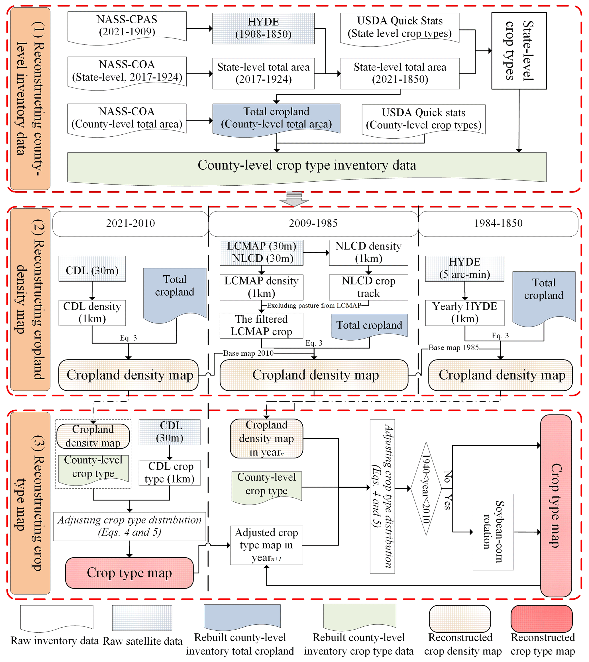
Figure 1 The methodology flow chart. The three boxes with red dashed lines correspond to Sect. 2.2, 2.3, and 2.4, respectively. The county-level total and crop-specific cropland area generated in the box (1) are fed into box (2) and box (3) to reconstruct cropland density and crop type maps, respectively. The following abbreviations/acronyms are used in the figure: NASS-CPAS – Crop Production Annual Summary data from the National Agricultural Statistics Service of the USDA; NASS-COA – Census of Agriculture from the National Agricultural Statistics Service of the USDA; CDL – Cropland Data Layer; NLCD – National Land Cover Database; LCMAP – Land Change Monitoring, Assessment, and Projection; and HYDE – History database of the Global Environment 3.2 (Klein Goldewijk et al., 2017).

2.1 Datasets

Three inventory datasets and four gridded LCLUC datasets were used in this study (Table 1). Specifically, NASS-CPAS (Crop Production Annual Summary data from the National Agricultural Statistics Service of the USDA) and NASS-COA (Census of Agriculture from the National Agricultural Statistics Service of the USDA) provide the total cropland area in each state and each county. USDA-NASS Quick Stats was used to track the acreage of specific crop types. These inventory datasets were adopted to reconstruct the historical crop-specific planting area for each county from 1850 to 2021, which served as a benchmark for adjusting the spatial maps in terms of planting acreage. CDL is the most detailed satellite-based cropland dataset for the period of 2010–2021, which has been intensively validated by ground truths and other ancillary data with crop classification accuracies of up to 90 % for major crop commodities (Boryan et al., 2011; Yu and Lu, 2018). Here, we extracted 10 crop types (Table S1 in the Supplement) from CDL. We compared the planting area between inventory data and CDL for nine crop types across counties from 2010 to 2021 (Fig. S1 in the Supplement). For most counties (>75 %), the residuals (the inventory-based crop area minus the CDL-based crop area) are less than 10×10³ ha (kha) for durum wheat, whereas they are less than 5 kha for other crops. NLCD and LCMAP, both derived from Landsat images with a resolution of 30 m × 30 m, were integrated to provide spatial information on the cropland distribution from 1985 to 2009. NLCD crop area is highly consistent with CPAS and COA, except that the crop area was significantly underestimated in NLCD 1992 (Fig. 4 in Yu and Lu, 2018), so it was excluded from the reconstruction of historical crop maps (Johnson, 2013). Due to its consistency with respect to cropland area, we utilized NLCD to identify the spatial distribution of cropland (Homer et al., 2020). However, NLCD provides around 5-year cyclical land cover maps from 2001 to 2019 (Homer et al., 2020). LCMAP offers annual land use data from 1985 to 2021. LCMAP adopts an Anderson Level-I-based legend, grouping cropland and pasture into one category (Xian et al., 2022). In contrast, NLCD uses an Anderson Level-II-based legend in which cropland and pasture are separately tracked (Table S4; Xian et al., 2022). To generate a reliable cropland distribution, the long-term non-crop trajectory derived from NLCD was used to exclude all grids identified as cropland from the LCMAP map (more details are presented in “Supplementary Methods: (1) Preprocesses for LCMAP” in the Supplement). For the period of 1850–1984, although both ZCMAP (the US cropland map from Zumkehr and Campbell, 2013) and HYDE provide the cropland distribution, HYDE considers the impacts of various environmental factors (soil suitability, temperature, and topography) on crop distribution compared with ZCMAP (Goldewijk, 2001; Goldewijk et al., 2011; Klein Goldewijk et al., 2017; Zumkehr and Campbell, 2013). Consequently, HYDE (available every 10 years) was initially used to identify the cropland distribution by calculating the fraction of cropland to the physical area for each grid. We further linearly interpolated the fraction for the missing years between 2 available years to provide a potentially continuous cropland distribution (more details are presented in “Supplementary Methods: (2) Linear interpolation in HYDE” in the Supplement). Here, all gridded datasets were resampled to 1 km. We employed a 1 km × 1 km window to aggregate the total cropland area from the 30 m × 30 m map and assigned the area to the corresponding 1 km × 1 km grid. To resample the CDL crop type map from 30 m to 1 km, the crop type in each 1 km × 1 km pixel was assigned to the dominant crop type with the largest fraction of land area within the 1 km × 1 km window. In addition, the cropland percentage in each 5 arcmin grid is interpolated to 1 km × 1 km grid cells with an assumption that cropland percentage is evenly distributed within the 5 arcmin × 5 arcmin window.

Table 1 The gridded and inventory dataset sources.

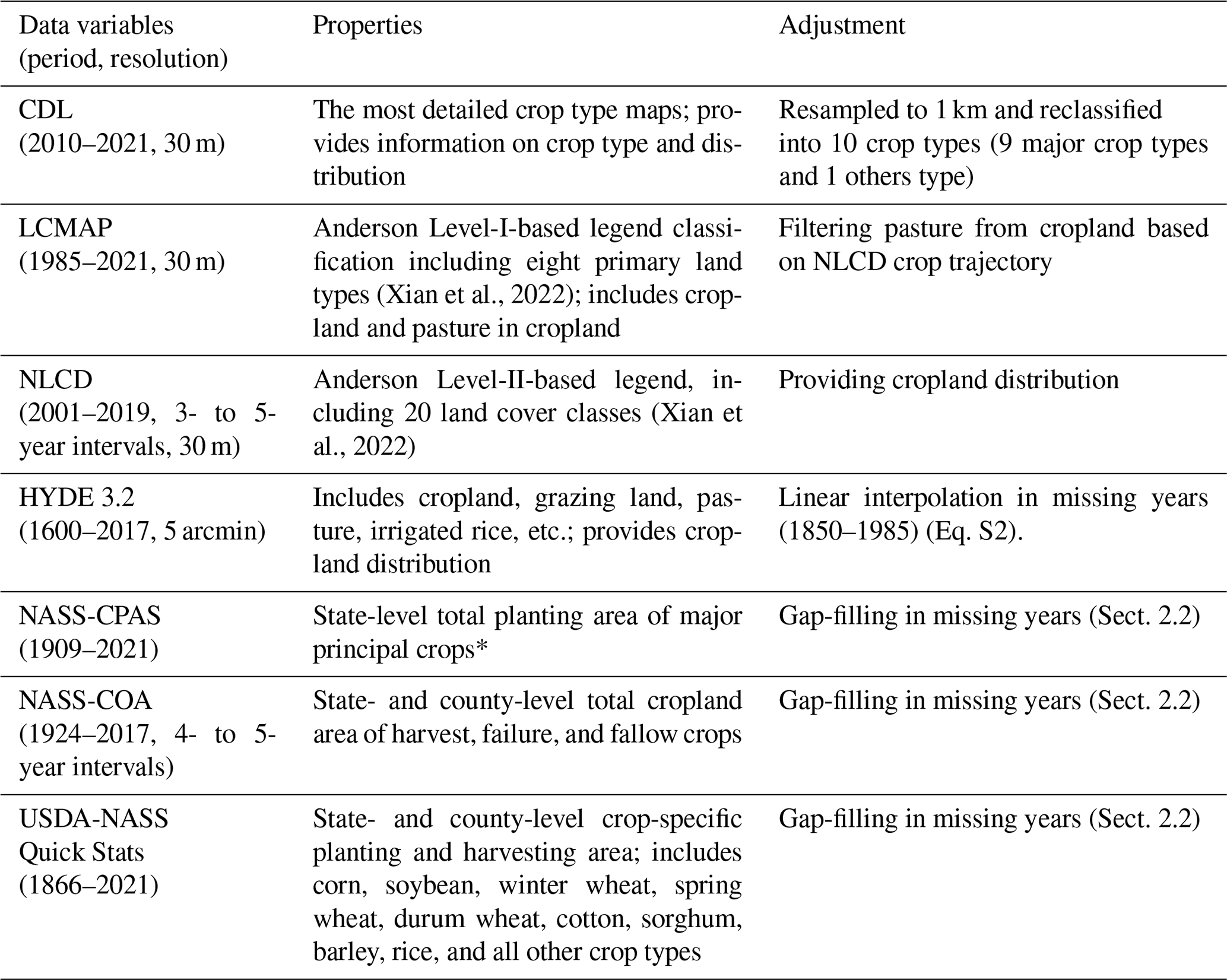
* Principal crops refer to grains, hay, oilseeds, cotton, tobacco, sugar crops, dry beans, peas, lentils, potatoes, and miscellaneous crops.

2.2 Reconstructing crop acreage history at the county level

By integrating and gap-filling multiple inventory and gridded datasets, we reconstructed the county-level time series of planting area and the planting area for nine major crop types and other crops from 1850 to 2021. Our reconstruction process was initiated with the development of crop-specific planting areas at the state level. NASS-CPAS reports the annual total planting area of major crops for each state from 1909 to 2021. However, some minor crop types, such as vegetables and fruits, are excluded. USDA-COA provides the total areas of crop harvest, failure, and fallow for each state from 1925 to 2017 at 4- to 5-year intervals. We computed the difference between these two datasets for available years and linearly interpolated unavailable years during 1909–2021. The difference was assumed to be the planting area of those minor crops. The interpolated difference was then added back to NASS-CPAS to generate the annual state-level total crop-planting area of all crops from 1909 to 2021. We used the interannual variations in arable land of each state extracted from HYDE to extrapolate the total planting area from 1908 to 1850 (Eq. 1). To identify the planting acreage change for nine major crop types, we obtained the state-level crop-specific harvesting and planting area from USDA-NASS Quick Stats. The available harvesting and planting areas vary among crop types and states, for which the harvesting areas usually have earlier-year reports than those of planting areas (Table S2). The harvesting area is highly correlated to the planting area in terms of interannual variation. We calculated the ratio of planting area to harvesting area for the earliest available year of planting area. We then converted the harvesting areas to planting areas by timing the ratio with the harvesting areas to extend the planting areas to an earlier period. For the period that the harvesting areas are unavailable, we interpolated the planting area from 1850 to 2021 based on the total planting area generated above as a referenced trend. Equation (1) was used when only the beginning or the ending year of the period was available, while Eq. (2) was used when both beginning and ending years were available. The planting area of “others” was obtained by calculating the difference between the total planting area and the summation of planting area of nine major crops.

We adopted the same approach as for the state-level planting area generated above to obtain the county-level total planting area and the planting area of nine major crop types and 1 others type. USDA-COA reports the total county cropland area from 1925 to 2017 at 4- to 5-year intervals. We gap-filled the total county planting area from 1850 to 2021 by using the state total planting area as a referenced trend (using Eq. 1 for gap-filling in cases where only the beginning or ending year was available or Eq. 2 in cases where both beginning and ending years were known). Similar to the state-level crop-specific planting area, we converted the harvesting areas to planting areas of nine major crops in each county from USDA-NASS Quick Stats, with varied availability (Table S2). For the period when harvesting areas were unavailable, we gap-filled the planting areas of each crop during 1850–2021 based on the state-level crop-specific planting area generated above as a referenced trend (Eqs. 1 and 2). The planting area of all other crops (others) in each county was estimated by calculating the difference between the total cropland area and the total area of nine major crops.

$$\begin{array}{}\text{(1)}& {\displaystyle }{\text{Raw data}}_{i+k}={\displaystyle \frac{{\text{Referenced trend}}_{i+k}}{{\text{Referenced trend}}_i}}\times {\text{Raw data}}_i\text{(2)}& {\displaystyle }\begin{array}{rl}{\text{Raw data}}_{i+k}& ={\displaystyle \frac{{\text{Referenced trend}}_{i+k}\times {\text{Raw data}}_i}{{\text{Referenced trend}}_i}}\times {\displaystyle \frac{k-i}{j-i}}\\ & +{\displaystyle \frac{{\text{Referenced trend}}_{i+k}\times {\text{Raw data}}_j}{{\text{Referenced trend}}_j}}\times {\displaystyle \frac{j-k}{j-i}}\end{array}\end{array}$$

Here, “Raw data” represents the raw data that contain missing values, “Reference trend” refers to the complete data from which the interannual variations can be used to derivate Raw data, i and j are the beginning and ending year of the gap, and i+k is the kth missing year.

2.3 Spatializing the county-level cropland density

By incorporating the county-level inventory (Sect. 2.2) and gridded cropland products, we reconstructed annual cropland density maps with a 1 km × 1 km resolution to represent the area and distribution of cultivated land in the conterminous US from 1850 to 2021. This process was divided into three periods: 2010–2021 (P2010), 1985–2009 (P1985), and 1850–1984 (P1850). CDL, LCMAP, and HYDE were used to provide the potential cropland distribution in P2010, P1985, and P1850, respectively. For the initial density maps in P2010 and P1985, we used a 1 km window to count the cropland fraction in each grid resampled from the raw CDL and LCMAP (30 m × 30 m), respectively, while initial annual density maps in P1850 were resampled and linearly interpolated from the HYDE maps. The pixel value in the resampled density map, representing the proportion of the cultivated land over the total pixel area, was further corrected based on the reconstructed county-level inventory data (Eq. 3).

Specifically, when the total cropland area in a county from the initial density map is larger than that of the inventory area, the extra area from all grid cells in the initial map would be deducted to maintain consistency with the magnitude of the inventory data; on the contrary, if the cropland area was less than the inventory data, the inadequate area would be added to all pixels (Yu and Lu, 2018). If the fraction in a grid is reduced below zero, the cropland fraction in that grid is assigned to zero and the remaining difference area between the map and the inventory data is subtracted from other grids. Conversely, if the fraction in a grid increases above 1 (100 %), then the value in that grid is assigned to 1, and the remaining area will be added to other grids.

$$\begin{array}{}\text{(3)}& {\text{AdjPixel}}_k={\text{Pixel}}_k+{\displaystyle \frac{\left(\text{inv}-\sum _{\mathrm{1}}^n{\text{Pixel}}_k\right)}{n}}\end{array}$$

Here, n is the total number of valid cropland pixels in a county; k is the pixel ID in that county, which is from 1 to n; inv is the inventory crop area in that county; Pixel_k is the initial cropland density in pixel k; and AdjPixel_k is the adjusted cropland density in pixel k.

To eliminate the gap between CDL and LCMAP, we used the adjusted CDL 2010 density map as a baseline map to retrieve the cropland density maps during 1985–2009 by adopting the year-to-year gridded changes from the resampled LCMAP maps. Taking the year 2009 as an example, the interannual difference in each grid between LCMAP 2009 and 2010 was applied to the adjusted CDL 2010 to generate the potential crop density map in the year 2009. Then, the potential density map was further corrected by the inventory data through Eq. (3). Following the same rule, the difference between the interpolated HYDE 1985 and 1984 was applied to the adjusted LCMAP 1985 to retrieve the density maps in P1850.

2.4 Spatializing the county-level crop type map

Based on the reconstructed county-level crop type inventory data (Sect. 2.2), corrected cropland density maps (Sect. 2.3), and CDL, the process of spatializing annual crop type maps was divided into two periods: 2010–2021 (P1) and 1850–2009 (P2). For P1, the raw 30 m resolution CDL crop type maps were resampled to 1 km to provide the potential crop type distribution. In this process, we assigned the resampled grid to a type with the largest percentage in a 1 km window. By integrating resampled crop type maps and reconstructed cropland density maps, we counted the total area for each type at the county level and identified the crop types whose area was greater than the corresponding inventory record. We further converted the surplus pixels from these types to other types whose area was less than inventory data (Eqs. 4 and 5). In particular, to avoid a grid planted by a fixed type for a long time, the surplus pixels were randomly selected for the conversion across different crop types. For P2, we assumed that the crop type pattern in 2 consecutive years would not change significantly and used the rebuilt crop type map in year_i+1 to provide the potential crop type distribution in year_i. Then, we followed the same rule in P1 to reconstruct the crop type map in year_i.

$$\begin{array}{}\text{(4)}& {\text{AdjType}}_j={\text{inv}}_j-\sum _{\mathrm{1}}^n\left({\text{AdjPixel}}_{j_k}\right)\end{array}$$

Here, inv_j is the inventory area of type j in a specific county; AdjType_j is the crop area to be converted among crop type j and other crop types; AdjPixel_jk is the adjusted cropland percentage in pixel k of crop type j; n is the number of total valid pixels of crop type j; and k is the pixel ID of crop type j, ranging from 1 to n, identified from the initial crop type map. For year_i between 2010 and 2021, the initial crop type map is resampled from CDL. For year_i from 1850 to 2009, the initial crop type map is the adjusted crop type map in year_i+1.

$$\begin{array}{}\text{(5)}& \left\{\begin{array}{l}{\text{Converting the area of AdjType}}_j\text{ from type }j{\text{ to other types, if AdjType}}_j<\mathrm{0};\\ {\text{Converting the area of AdjType}}_j\text{ from other types to type }j,{\text{ if AdjType}}_j>\mathrm{0}.\end{array}\right.\end{array}$$

Considering the dominant crop rotation type in the US, soybean–corn rotation, we simulated the corn–soybean rotation by randomly switching a certain area between corn and soybean according to the rotation rate. The crop rotation information from 1996 to 2010 at the state level was documented by the “Tailored Reports: Crop Production Practices” of USDA's Agricultural Resource Management Survey (ARMS) (https://data.ers.usda.gov/reports.aspx?ID=17883, last access: 20 July 2024). The rotation rate was calculated as the ratio of the sum of corn–soybean and soybean–corn acreage to the total area of corn and soybean. We found that the rotation rate in each state remained relatively stable in the ARMS-available years and, thus, assumed that the rotation rate in the missing years was the same as the mean rate from available years (Table S3), which was further applied to corresponding counties. Because soybean was rarely planted in the Corn Belt before 1940 (Yu et al., 2018), we only considered the corn–soybean rotation during the period 1940–2009 in 17 states (Table S3; Padgitt et al., 1990).

2.5 Evaluation method

Here, we adopted multiple indexes to evaluate the crop area discrepancy between the reconstructed maps and inventory data at various scales. At the county level, we utilized the residual (resd_ij) and relative residual (relative_resd_ij) to describe the crop area difference and the relative difference between the rebuilt maps and the inventory data (Eqs. 6 and 7). In addition, at the national scale, the root-mean-square error (RMSE) and R-squared (R²) are used to assess the crop area consistency between the crop maps and the inventory data.

$$\begin{array}{}\text{(6)}& {\displaystyle }{\text{resd}}_{ij}={\text{inv}}_{ij}-{\text{map}}_{ij}\text{(7)}& {\displaystyle }{\text{relative\_resd}}_{ij}=({\text{inv}}_{ij}-{\text{map}}_{ij})\cdot \mathrm{100}/{\text{inv}}_{ij}\end{array}$$

Here, inv_ij and map_ij are the crop area derived from the inventory data and the rebuilt maps at year i in county j, respectively, and resd_ij and relative_resd_ij are the residue and relative residue at year i in county j, respectively.

2.6 Cropping diversity analysis

Cropping diversity has been identified as a potential factor affecting crop yield (Renard and Tilman, 2019; Driscoll et al., 2022). Here, we adopted a true diversity index proposed by Jost (2006) to analyze the US crop diversity pattern. The true diversity (D) quantifies the effective number of crop species (Eq. 8), where a given D value is equivalent to the number of crop species with an equal area in a certain space. D is calculated as the exponent of Shannon diversity index (H).

$$\begin{array}{}\text{(8)}& D=\exp \left(-{\sum }_{j=\mathrm{1}}^n(P_j\cdot \ln P_j)\right)=\exp \left(H\right)\end{array}$$

Here, P_j is the proportion of the cropland area occupied by the crop type j over the total cropland area and n is the number of crop species. In this study, the diversity calculated involves 10 crop types, including 9 major crop types and an others category.

3 Result

3.1 Validation of the data products

In this study, we adopted the inventory data to refine the gridded map, recognizing that achieving exact alignment for each crop type within each county might be challenging due to constraints related to the limited cropland area available for allocation. Here, we examined the crop-specific area alignment between the inventory data and our map products at multiple scales. We compared the annual crop-type-specific acreage extracted from our maps with the raw inventory data at the county level in 1920, 1960, 2000, and 2020 (Fig. S2). The county-level acreages derived from our products and inventory data are close to the 1:1 line, with an R² value exceeding 0.95 and an RMSE <1 kha for all of the major crop types except for winter wheat (R²=0.98, RMSE = 2.79 kha) and cotton (R²=0.95, RMSE = 3.97 kha). Although winter wheat and cotton present a relatively greater RMSE, the counties with a crop area bias greater than 10 % only account for 9.7 % and 6.1 % of total winter wheat- and cotton-planting counties in the selected 4 years, respectively. We further examined the time-series residual between the inventory data and maps (Figs. 2 and S3). It is evident that the residuals (the inventory-based crop area minus the rebuilt-map-based crop area; Eq. 6) are generally smaller than 0.2 kha for the majority of counties (>75 %) across all years for nine crop types. Relatively greater residuals are observed in spring wheat, durum wheat, and rice before 1875 (Fig. 2d, g, and i), which might be attributed to the marginal area of these three crops during the early years. Similarly, the relative errors (the ratio of residual to the inventory crop area; Eq. 7) in most counties remain within ±2 % for different crops, except for spring wheat, durum wheat, and rice before 1875 (Fig. S3d, g, and i). We also checked the consistency in national crop-specific acreage between our maps and the inventory data during 1850–2021 (Fig. S4). The results show that the map products match well with the inventory data (R² close to 1 and RMSE <0.3 Mha for all crop types), indicating that the developed maps are highly consistent with the inventory data at a national scale. The multiscale validations demonstrate that the developed dataset has a strong capacity to capture the interannual crop-specific area variation.

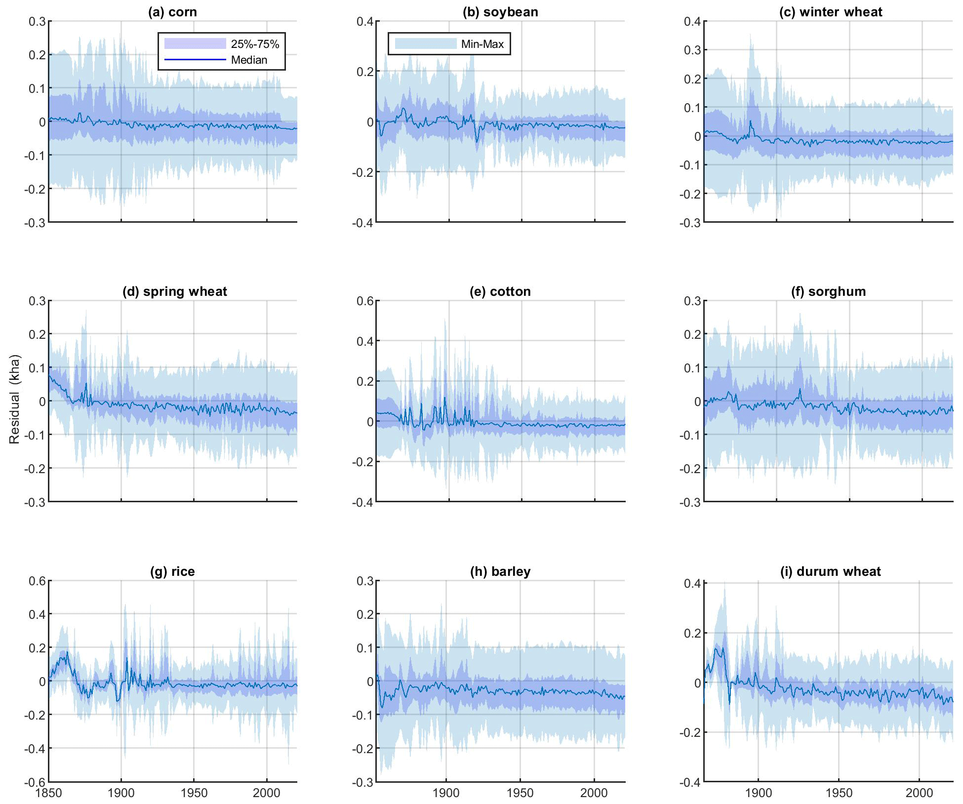
Figure 2 The distribution of residual (the inventory-based crop area minus the rebuilt-map-based crop area, defined by Eq. 6) between the rebuilt inventory and maps from 1850 to 2021 (kha is a thousand hectares). In each year, “Min–Max”, “Median”, and “25 %–75 %” reflect the extent of residual from all counties at levels of “minimum value to maximum value”, “50th percentile”, and “25th percentile to 75th percentile”, respectively.

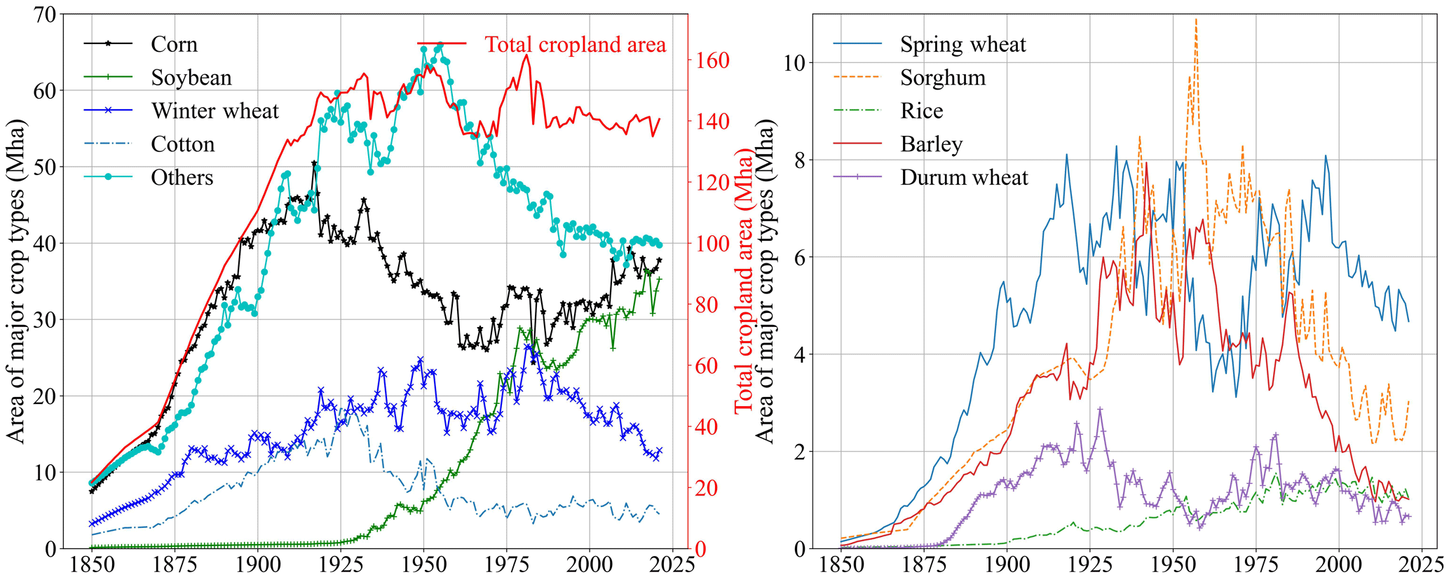
We examined the historical changes in cropland area among various crop types in the US from 1850 to 2021 (Fig. 3). In general, the US cropland expanded rapidly from 21.66 Mha in 1850 to 149.28 Mha in 1919, followed by a wide fluctuation ranging from 134.78 to 161.80 Mha until 1990, and then remained relatively stable at around 140.00 Mha until 2021. Corn was the dominant crop in the US, accounting for more than 20 % of the national total cropland area throughout the study period. Temporally, it rose sharply from 7.47 Mha in 1850 to 50.47 Mha in 1917, followed by a continuous drop to 26.26 Mha until 1962, and slowly increased to 37.75 Mha during 1962–2021. Soybean soared significantly from 4.35 Mha in the 1940s to 35.25 Mha in 2021, becoming the second most extensive crop type in the US. Winter wheat constantly increased from 3.25 Mha in 1850 to 26.43 Mha in 1981 and then dropped to 12.88 Mha in 2021, while spring wheat fluctuated dramatically after it plateaued at 8.28 Mha in 1933. Barley and sorghum climbed to peaks of around 8 Mha in the 1940s and 11 Mha in the 1950s and then dropped to about 1 and 3 Mha by 2021, respectively. Furthermore, cotton and durum wheat both reached their peaks before the 1930s and then fell to a relatively stable level. Throughout the study period, the total US cropland increased by 118 Mha, predominantly driven by corn (30 Mha), soybean (35 Mha), and others (31 Mha). The remaining row crops shared about 18 % of this increase, including winter wheat (9.6 Mha), spring wheat (4.5 Mha), sorghum (2.8 Mha), cotton (2.7 Mha), and rice (1 Mha).

Figure 3 Annual area of major crop types and total US cropland area from 1850 to 2021.

3.2 Dynamics of cropland distribution

The spatial patterns of cropland density and crop type are presented in Fig. 4. Generally, the hot spots of cropland are concentrated in the Midwest and Great Plains regions (the spatial pattern of US subregions shown in Fig. 5.2-a), starting from 1950, where large crop field sizes were likely to occur (Yan and Roy, 2016). The results show that the cropland was mainly distributed in the eastern region of the US in 1850 with a low distribution percentage (<40 %) (Fig. 4a). Then, the cropland density enhanced substantially (40 %–80 %) in 1900 (Fig. 4b). Meanwhile, a large area of the Great Plains was cultivated to plant corn and spring wheat in the Northern Great Plains and winter wheat in the Southern Great Plains during 1850–1900 (Fig. 4f). From 1900 to 1950, the cropland fraction was continuously elevated (>60 %) (Fig. 4c), especially in the Midwest and the Great Plains. During 1950–2021, the cropland fraction further increased in the US Midwest but decreased in the Southeast. Moreover, the others category substantially substituted corn, winter wheat, and cotton in the US Southeast and, therefore, lowered the cropland density in this region (Fig. 4d). It was noted that soybean has increased tremendously in the US Midwest, the Dakotas, and the Rice Belt since 1950, replacing parts of spring wheat, winter wheat, barley, and rice in these regions. Overall, the hot spots of US cropland have shifted from the Eastern US to the Midwest and the Great Plains with the increasing cropland percentage over the past 170 years.

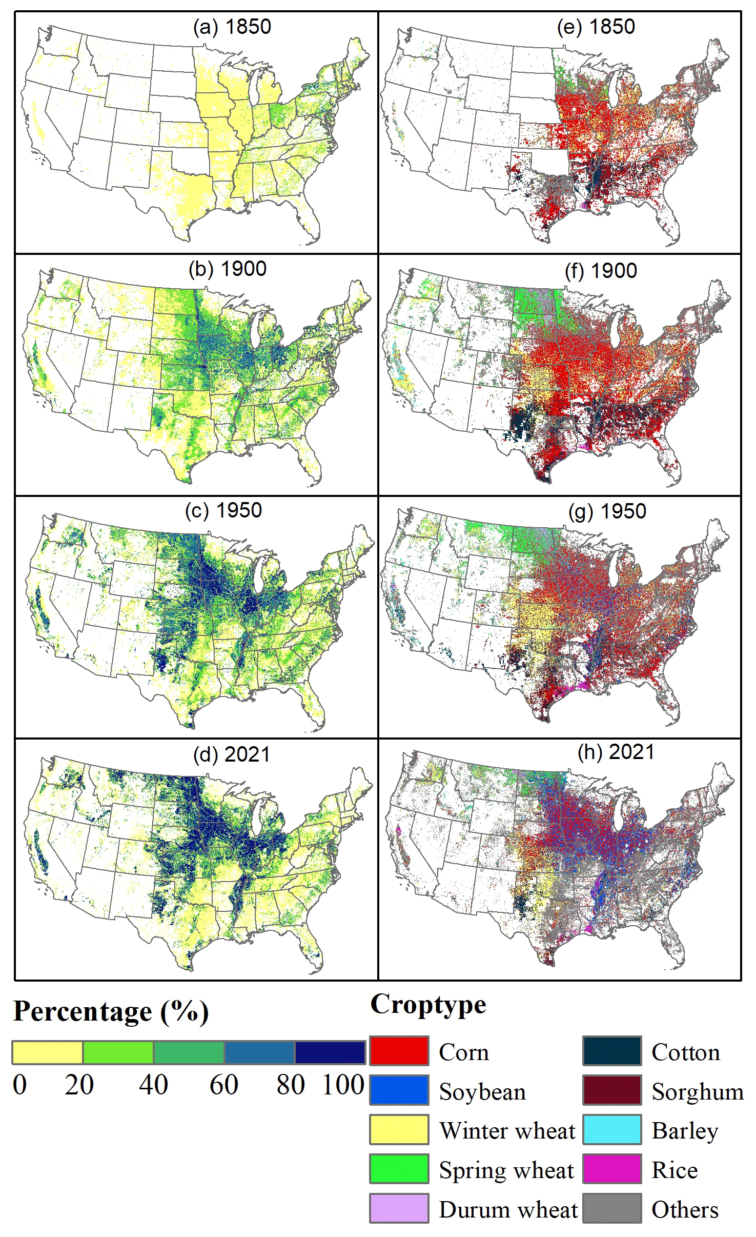
Figure 4 The spatial patterns of cropland percentage (a–d) and dominant crop type (e–h) at a 1 km × 1km resolution in 1850, 1900, 1950, and 2021. The color bar of “Percentage” indicates the percentage of planting area to the grid area. “Others” represents the remaining crop types.

Furthermore, the spatiotemporal patterns of each major crop type were examined in this study to present a systematic understanding of the US cropland extent and type changes (Figs. 5, S5, and S6). Specifically, corn was mainly planted in the east in 1850, with a low cropland fraction (<40 %) (Fig. 5.1-a). Then, it gradually expanded to the Great Plains, and the total area increased by 43 Mha from 1850 to 1917. Meanwhile, the hot spots of corn-planting areas shifted to the US Midwest, the southeast of the Northern Great Plains, and the northeast of the Southern Great Plains (Fig. 5.1-b). From 1917 to 1962, the spatial extent of corn had shrunk in South Dakota, Nebraska, Kansas, and the US Southeast, with a total area decrease of 24.21 Mha (Fig. 5.1-c). Although the US Southeast experienced a large decline in corn acreage during 1962–2021, the planting density of corn significantly increased in the US Midwest and the southeast of the Northern Great Plains, resulting in the corn area peaking at 37.75 Mha in 2021 (Fig. 5.1-d).

Temporally, soybean was rarely cultivated in the US from 1850 to 1900, with a total area less than 1 Mha (Fig. 5.2-a and 2-b). During 1900–1940, the planting area of soybean had a small expansion in the US Midwest, with a total area rising to 4.35 Mha (Fig. 5.2-c). However, it then had a dramatic expansion from 1940 to 2021 to the US Midwest, Southeast, and the east of Northern Great Plains, with the total soybean area increasing to 35.25 Mha (Fig. 5.2-d).

Winter wheat was mainly located in the US Midwest in 1850 with a total area of 3.25 Mha (Fig. 5.3-a). In the following 5 decades, it spread to the Great Plains, California, Washington, and Oregon, with the total area increasing to 14.45 Mha in 1900 (Fig. 5.3-b). From 1900 to 1981, although its spatial extent had shrunk in the US Midwest, it expanded significantly in the Southern Great Plains, the US Southeast, and Montana (Fig. 5.3-c). Meanwhile, the cropland density also enhanced in this period. These changes led to the planting area of winter wheat reaching a peak of 26.43 Mha in 1981. However, during 1981–2021, a large area of winter wheat was replaced by other crop types or other land use types in the US Midwest, Southeast, Montana, Washington, and California (Fig. 5.3-d), which reduced the total area of winter wheat to 12.88 Mha in 2021.

Cotton was mainly distributed in the US Southeast in 1850 with a low density (Fig. S5.1-a). It sharply expanded to the Southern Great Plains and California with an increased density during 1850–1925 (Fig. S5.1-b), and the total area of cotton increased by 16.53 Mha in this period. However, the period of 1925–2021 was characterized by a huge contraction of cotton area in the US Southeast and Southern Great Plains, with a total area declining to 4.50 Mha (Fig. S5.1-c and 1-d).

For spring wheat, there was a significant expansion from Montana and Wisconsin to the US Midwest and Northwest during 1850–1933, resulting in a total area increase to 8.28 Mha (Fig. S5.2-a and 2-b). However, the distribution of spring wheat largely shrunk in the US Midwest and Northwest from 1933 to 1969 (Fig. S5.2-b and 2-c), resulting in the area decreasing to 3.11 Mha. In recent decades, it has mainly been centered in the northern part of the Northern Great Plains with the enhanced density in each grid, and its total area increased to 4.67 Mha in 2021 (Fig. S5.2-d).

Sorghum consistently expanded in the Southern Great Plains from 1850 to 1957, with its total area increasing by 10.70 Mha (Fig. S6.1-a to 1-c). However, there was a subsequent area decline thereafter, leaving the total at 3.03 Mha in 2021 (Fig. S6.1-d). Similarly, barley experienced a continuous expansion in the US Midwest, Great Plains, Northeast, California, and Colorado, with the total area rising from 0.06 Mha in 1850 to 7.94 Mha in 1942 (Fig. S6.2-b to 2-c). However, between 1942 and 2021, the distribution of barley underwent a dramatic contraction across the entire US and shrank to 1.02 Mha in 2021, with a small extent in the Northern Great Plains (Fig. S6.2-d).

Compared with other major crop types, both the distribution of durum wheat and rice only occupied a small area of the US over the entire study period (<3 Mha). Specifically, durum wheat underwent significant expansion in North Dakota and South Dakota from 1850 to 1928 (Fig. S5.3-a and 3-b), reaching a peak area of 2.86 Mha in 1928. Subsequently, it contracted to the eastern part of North Dakota during 1928–1958, with the total area declining to 0.42 Mha (Fig. S5.3-c). From 1958 to 2021, its planting area shifted to the junction of North Dakota and Montana (Fig. S5.3-d). Rice consistently expanded in Arkansas, Louisiana, Mississippi, and Texas from 1850 to 1981, resulting in a total area increase of 1.55 Mha (Fig. S6.3-a to 3-c). This expansion gradually formed the current Rice Belt pattern, followed by a small shrinkage (0.52 Mha) in these regions between 1981 and 2021 (Fig. S6.3-d). The others category includes various minor crop types, such as peanuts, oats, and alfalfa, collectively accounting for 27 %–43 % of the total US cropland area and being distributed across the entire US (Fig. S7).

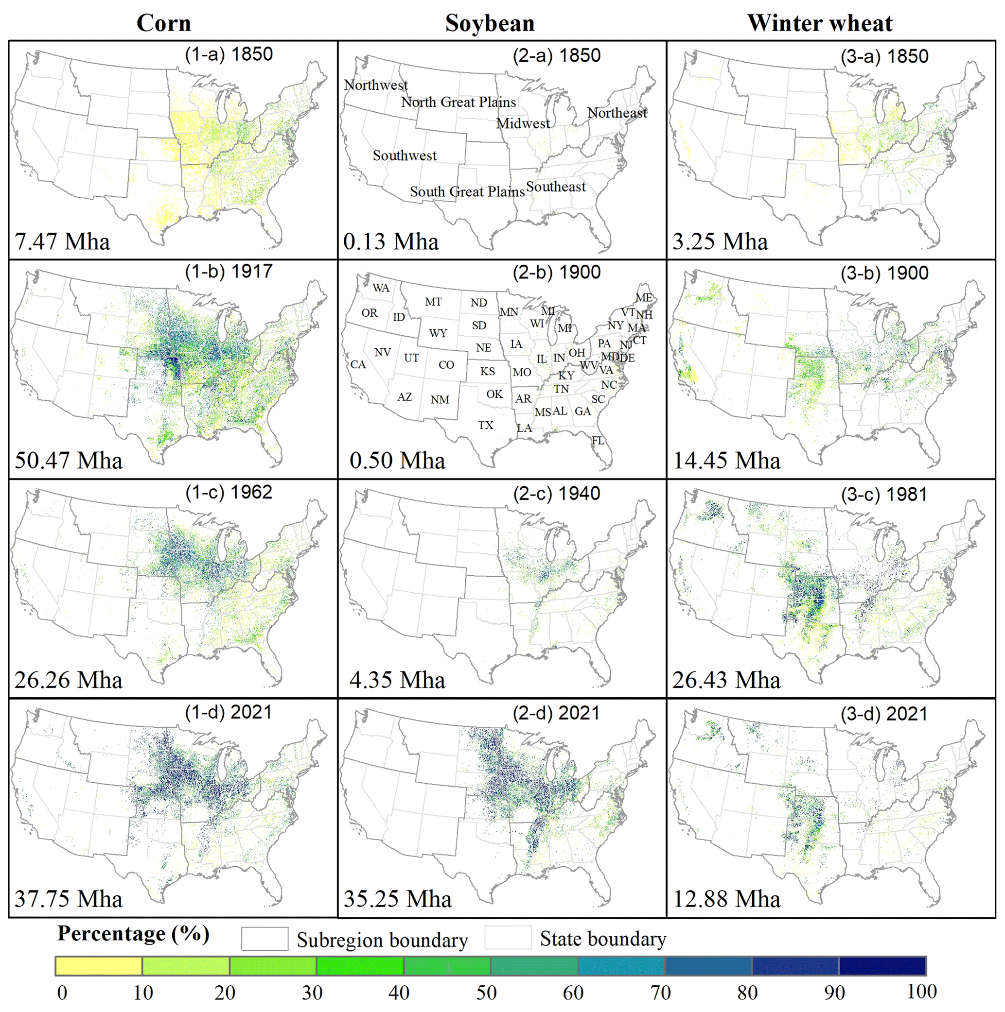
Figure 5 The spatial density pattern of corn, soybean, and winter wheat at a 1 km × 1 km resolution in the turning point years with abrupt area changes. The first, second, and third columns are the density patterns of corn, soybean, and winter wheat, respectively. The total planting area for each crop type is presented in the bottom left of each panel. The color bar at the bottom indicates the percentage of planting area to the total grid area.

3.3 Changes in cropping diversity over time

Here, the value of true diversity (D) is interpreted as the number of crop species with an equal area in a certain space (Jost, 2006; Hijmans et al., 2016); thus, a higher D value means more crop types, a more even distribution, or both. As shown in Fig. 6, the US cropping system diversity has undergone dramatic change over time, with a sharp increase from 1850 to 1963 and a significant decline in the recent 60 years. Among different regions, the US Southwest, Northern Great Plains, Southern Great Plains, and Southeast had a higher cropping diversity system than the remaining regions. Specifically, the diversity in the US Southwest, Southern Great Plains, and Northern Great Plains presented a similar change during the 1850s–1940s, with a drop from the 1850s to the 1880s followed by an obvious increase to the 1940s (Fig. 6b). Starting from the 1940s, the diversity in the Northern Great Plains peaked around the 1990s and then constantly decreased to 2021, while the Southern Great Plain's diversity presented an opposite trend in this period. Meanwhile, the US Southwest witnessed a continuous decline in crop diversity from the 1940s to the present. The US Southeast retained stable diversity during the 1850s–1930s and then experienced a significant increase from the 1940s to the 2000s. However, in the recent 20 years, the diversity in the US Southeast has dropped sharply. The diversity in the US Northeast has shown an increasing trend across the entire study period. The crop diversity in the US Northwest fluctuated between 2.5 and 3 from the 1850s to the 1970s and then had a continuous increase to the present. The US Midwest's crop diversity remained relatively stable during the 1850s–1920s. After increasing to its peak between the 1920s and the 1930s, it remained stable from the 1930s to the 1980s, followed by a dramatic decrease to 2021.

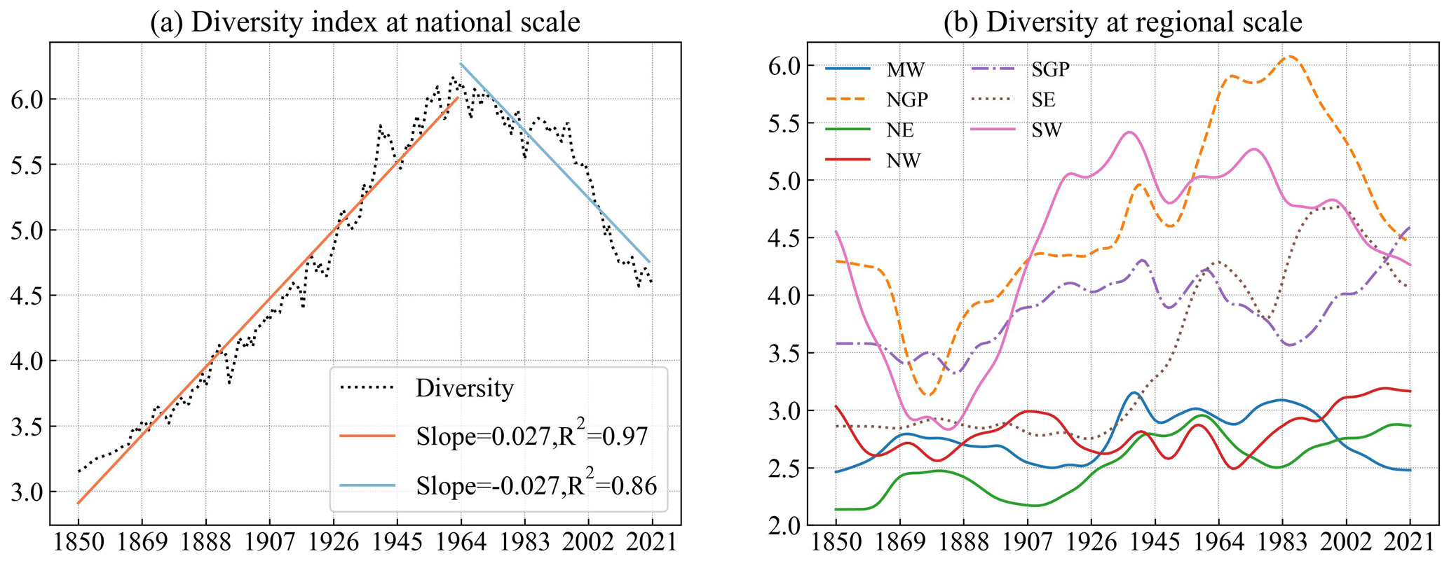
Figure 6 The temporal trend in the diversity value in the US (a) and seven regions (b). NW, SW, NGP, SGP, MW, SE, and NE represent Northwest, Southwest, Northern Great Plains, Southern Great Plains, Midwest, Southeast, and Northeast, respectively. The spatial map of the seven regions is presented in Fig. 5.2-b. To get a better visual pattern, the trends of the seven regions in panel (b) were smoothed by the Gaussian function. The diversity value is calculated based on the reconstructed inventory data.

4 Discussion

4.1 Comparison with other datasets

We systematically compared our product with previous datasets regarding the historical total cropland areas (Fig. 7) and their spatial patterns (Fig. 8) to provide a complete reference for potential applications. By combining NASS-CPAS and NASS-COA to reconstruct state- and county-level inventory data, the US total cropland area derived from our density maps matches well with that from NASS-CPAS from 1850 to 1940 and consistently aligns with the magnitude of NASS-COA and the interannual variations in NASS-CPAS between 1940 and 2021 (Fig. 7). We extracted the US total cropland area from two widely used geospatial satellite products (USDA-CDL and USGS-NLCD) in the most recent 2 decades. These two datasets demonstrate a smaller area than that of NASS-COA before 2017, but their estimation of crop area magnitude and interannual variation have presented greater consistency with this study over the most recent 5 years. Meanwhile, Yu and Lu (2018) and Li et al. (2023) all used NASS-CPAS to develop YLMAP and CONUS, respectively, resulting in a lower US total cropland area after 1940 than this study. This is because NASS-CPAS only includes the cropland area of principal crops in each state, which is lower than the total cropland area reported by NASS-COA, especially after 1940. Among the existing databases, LCMAP, HYDE, GBC, and ZCMAP represented an upper bound of the US total cropland area. Especially for GBC, it reported a national total crop acreage about 50 % higher than the upper range of all other data products (∼300 vs. ∼200 Mha around the 1980s in Fig. 7).

The divergence among these data products is mostly caused by different cropland definitions and cropland map generation processes. Spatially, we observed that HYDE exhibits broader cropland extent and a higher fraction of cropland per grid than our products, particularly in regions with low-density cropland distribution, such as the US Northwest, Southeast, and Southwest (Figs. 8 and 9). This disparity might be attributed to the definition of cropland in HYDE that includes both arable land and permeant cropland (Goldewijk, 2001), whereas our map exclusively accounts for the crop-planting area of crops. More importantly, the crop-planting area of our map was constrained based on county-level inventory data. Meanwhile, HYDE spatialized the subnational-level inventory data to allocate cropland area to each grid in accordance with “cropland suitability maps” informed by dynamical social (historical population density) and stable environmental (soil suitability, temperature, and topography) information (Goldewijk et al., 2011; Yu and Lu, 2018). As a result, greater acreage and a wider extent of cropland were estimated by HYDE and were allocated to each grid (Figs. 7, S8, and S9). Similarly, the category of cropland in LCMAP and ZCMAP contains crop and pasture (Zumkehr and Campbell, 2013; Xian et al., 2022), while GBC cropland refers to arable land (Klein Goldewijk et al., 2017; Cao et al., 2021), leading to their higher cropland area than our result (Fig. 7). Also, the grid density of ZCMAP was higher than this study in low-density regions (the first row in Fig. 9), as ZCMAP adopted an assumption that the historical spatial crop pattern remained roughly similar to the base map 2000, in which the fraction in each grid is higher in these regions (Ramankutty et al., 2008; Zumkehr and Campbell, 2013). Moreover, CONUS showed a more extensive cropland distribution than our maps (especially in the Great Plains and US Southeast; Fig. 8 and the third row in Fig. 9). This is likely because they produced more potential cropland grids than the county records through an artificial neural-network-based land cover probability occurrence model (Li et al., 2023). GBC feeds population density and eight biophysical variables (including elevation, temperature, and soil water) into a random forest model to generate the cropland distribution (Cao et al., 2021). As a result, the spatial pattern between GBC and our maps shows a high agreement at the national scale (Fig. 8). However, the cropland percentage in each grid cell of GBC is significantly higher than other maps (Fig. 8 and the second row in Fig. 9), which might be related to the base map used in their study and the lack of inventory records for limiting the total cropland area in the US (Cao et al., 2021).

In terms of spatial details among these datasets, our products, YLMAP, CONUS, and GBC (1 km × 1 km) can provide more detailed spatial information than HYDE and ZCMAP (5 arcmin) (Fig. 9). Furthermore, compared with YLMAP, CONUS, and HYDE, which incorporate state-level census, our products are likely to demonstrate more reliable cropland density heterogeneity within a state (the third row in Fig. 9), as we adopted county-level census to control the total cropland area in each county. Thus, the rebuilt map is capable of capturing spatial shifts between counties within the same state, such as cropland abandonment in some counties but expansion in others (Fig. 9). This indicates that the county inventory-derived datasets are more appropriate for subregion applications (Yang et al., 2020).

Overall, our product remains highly consistent with the county-level inventory data and presents a similar cropland distribution to YLMAP and GBC that involves both biophysical and socioeconomic drivers to generate crop pixels. In addition, unlike cropland involving arable land in HYDE or harvesting land in CONUS mentioned above, the definition of cropland in our product refers to the crop-planting areas and excludes idle and fallow farm land and cropland pasture, providing real surface information disturbed by agriculture. This improvement enhances the estimation of the effect of cropland change on the environment. Therefore, the developed maps can provide a more comprehensive cropland tracking for ecological and environmental assessment, covering both cropland distribution and crop types at national and regional scales.

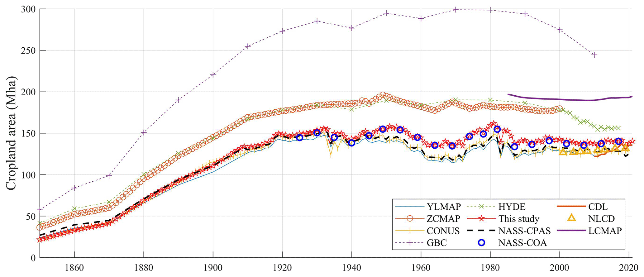
Figure 7 Comparison of the US total cropland area from different sources. The following abbreviations/acronyms are used in the figure: CDL – Cropland Data Layer; NLCD – National Land Cover Database; LCMAP – Land Change Monitoring, Assessment, and Projection; YLMAP – the US cropland map from Yu and Lu (2018); ZCMAP – the US cropland map from Zumkehr and Campbell (2013); CONUS – the cropland map from Li et al. (2023); GBC – the US cropland extracted from the global cropland dataset developed by Cao et al. (2021); HYDE – History database of the Global Environment 3.2 (Klein Goldewijk et al., 2017); NASS-CPAS – the Crop Production Annual Summary data from the National Agricultural Statistics Service of the USDA; and NASS-COA – the Census of Agriculture from the National Agricultural Statistics Service of the USDA. In particular, YLMAP, ZCMAP, CONUS, and GBC are not used in this study to reconstruct crop maps.

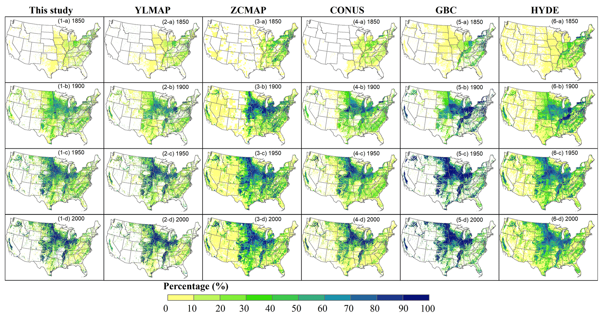
Figure 8 The spatial patterns of cropland from different datasets in the selected years of 1850, 1900, 1950, and 2000. The following abbreviations/acronyms are used in the figure: YLMAP (1 km) – the US cropland map from Yu and Lu (2018); ZCMAP (5 arcmin) – the US cropland map from Zumkehr and Campbell (2013); CONUS (1 km) – the cropland map from Li et al. (2023); GBC (1 km) – the US cropland extracted from the global cropland dataset developed by Cao et al. (2021); and HYDE (5 arcmin) – History database of the Global Environment 3.2 (Klein Goldewijk et al., 2017).

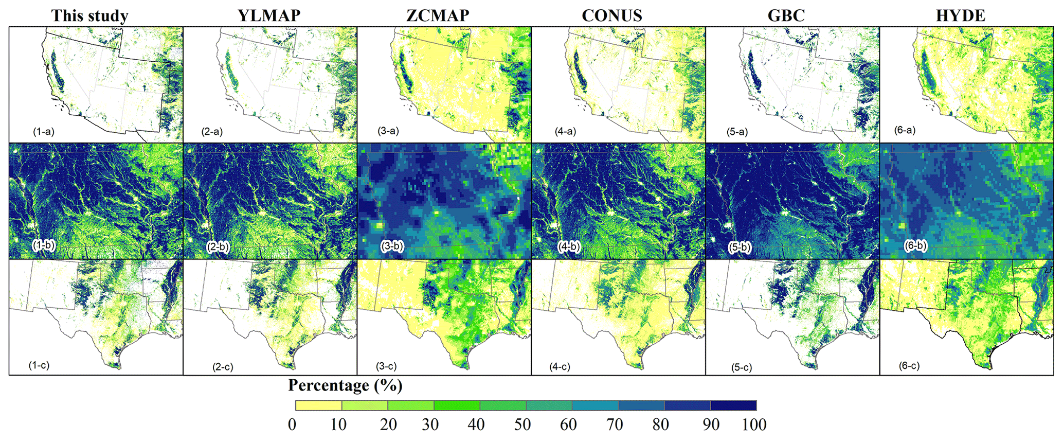
Figure 9 The detailed spatial pattern from different datasets in the year 2000. The following abbreviations/acronyms are used in the figure: YLMAP (1 km) – the US cropland map from Yu and Lu (2018); ZCMAP (5 arcmin) – the US cropland map from Zumkehr and Campbell (2013); CONUS (1 km) – the cropland map from Li et al. (2023); GBC (1 km) – the US cropland extracted from the global cropland dataset developed by Cao et al. (2021); and HYDE (5 arcmin) – History database of the Global Environment 3.2 (Klein Goldewijk et al., 2017). The spatial extent in each row for panels (a), (b), and (c) is for the US Southwest, Iowa, and Texas, respectively.

4.2 The drivers for US cropland change

Between 1850 and 1900, there was a notable cropland expansion toward the west (Fig. 4). This was mainly driven by the Homestead Act of 1862, which provided 160 acres of land to the public for farming purposes (Anderson, 2011). Additionally, the end of the Civil War, the disbanding of armies, and the building of canals and railroads toward the west further contributed to the agricultural market and export, accelerating agricultural reclamation (Ramankutty and Foley, 1999). At the same time, corn, cotton, and wheat were the dominant crop types and expanded rapidly to the west (Figs. 5 and S5). From 1900 to 1950, advanced irrigation systems, industrial technology, and mechanization further promoted agricultural development. For instance, the areas of winter wheat, sorghum, and barley increased substantially in this period (Figs. 5, S5, and S6). Subsequently, the fluctuation in the market, policy structure, and weather conditions played a dominant role in affecting the interannual variations in agricultural areas (Spangler et al., 2020). For example, the farm crisis in the 1980s resulted in a significant cropland drop. Moreover, a series of historical cropland acreage-reduction programs, such as the Conservation Adjustment Act Program and Conservation Reserve Program, resulted in a total cropland reduction (Lubowski et al., 2006). In the most recent 3 decades, the total US cropland has remained relatively constant, but the crop commodities have changed significantly. Corn and soybean have gradually become the predominant crop types due to the rising demand for corn as biofuel and the higher market price for soybean, which has pushed framers to convert other types to corn and soybean (Bigelow and Borchers, 2017; Aguilar et al., 2015). Overall, US cropland experienced significant growth between the 1850s and the 1920s, driven by population growth, industrialization, mechanization, and market change. It subsequently underwent a process of stabilization after experiencing fluctuations in crop types and area.

4.3 The implications for cropping diversity change

In general, the US cropping diversity experienced a dramatic change throughout the entire period. From 1850 to 1963, it constantly increased (Fig. 6a), primarily attributed to the rising areas of all major crop types during this stage (Fig. 3). Spatially, the diversity increases in the US Southwest, Southeast, and Great Plains contributed to the overall increase in the country's cropping diversity (Figs. 6b and 10). From the 1960s to 2021, the cropping diversity had a significant decrease, mainly due to the increased planting area of corn and soybean and the decreased cultivated area of winter wheat, spring wheat, sorghum, and barley. Meanwhile, the diversity drop in the US Northern Great Plains, Southwest, Southeast, and Midwest might contribute to the country's crop diversity decline (Figs. 6b and 10). This finding shows a strong agreement with the results of Aguilar et al. (2015), who found that the crop species diversity declined from the 1980s to the 2010s in the Midwest.

On the other hand, crop species diversity is an important component of biodiversity within a cropping system, and a decrease in crop species diversity is often associated with a decline in overall biodiversity (Altieri, 1999). Some researchers have pointed out that biodiversity plays an essential role in the functioning of the real-world ecosystem. High biodiversity would increase soil fertility, mitigate the impact of pests and diseases, improve resilience to climate change, and promote food production and nutrition security (Altieri, 1999; Duffy, 2009; Frison et al., 2011). For example, Renard and Tilman's research indicated that crop species diversity could stabilize food production (Renard and Tilman, 2019), and Burchfield et al. (2019) found that agricultural diversification can increase crop production. Thus, one could pose the following question: has the significant drop in the US cropping diversity over the past 6 decades affected yield and ecosystem productivity? Moreover, under more frequent climate extremes anticipated in the future, will decreasing cropping diversity affect the sustainability and resilience of the US agricultural system?

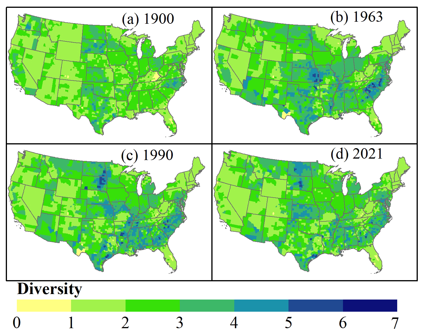
Figure 10 The spatial pattern of crop diversity in 1900, 1963, 1990, and 2021 at the county level. The diversity value is calculated based on the gap-filled and multisource harmonized inventory data in each county.

4.4 Uncertainty

In this study, we integrated the inventory data and the gridded LCLUC products to generate annual cropland density and crop type maps at a resolution of 1 km × 1 km from 1850 to 2021. Although our data are highly consistent with inventory data, some uncertainties remain:

1. In the upscaling process of CDL from 30 m to 1 km, we assigned each pixel to a dominant crop type with the biggest fraction of land area within the pixel. Although the area of each crop was constrained by the inventory data at the county level, this resampling process may overlook certain crop type distributions with a minor fraction within a pixel.

2. The inventory is crucial for reconstructing historical cropland maps. Here, the rebuilt inventory data in missing years are interpolated. Although this study is based on our best knowledge, this method may not reflect the real interannual cropland area fluctuations in the missing years.

3. In the process of spatializing crop types, we randomly convert the cropland grids from specific types with higher map area than inventory data to other crop types within each county. In addition, grids identified with corn–soybean rotation were randomly selected within a county based on the corn–soybean rotation ratio, aiming to prevent a grid cell from being consistently occupied by a single crop type over time. While the extent of the random processes varied among counties based on the difference between intermediate map data and inventory data, it is important to note that they may influence the temporal trajectory of grid-based crop type changes. Thus, users should proceed with caution when employing this data product for time-sequencing analyses, such as crop rotation patterns (e.g., continuous corn or corn–soybean–corn) at the pixel level.

4. The diversity in this study mainly reflects the change in diversity among 10 crop types (9 major types and 1 others category). It is important to note that the others category in the study is not a single crop type, rather a combined category including various minor crop types (peanuts, oats, etc.). Thus, the diversity changes quantified in this study capture the diversity of major row crops (accounting for 70 % of the national total cropland area in the 2010s) and the “others-as-one-category” in the US over time. A more comprehensive diversity analysis involving all crop types would require a more detailed time-series crop type record, which is currently lacking.

5 Data availability

The developed dataset is available at https://doi.org/10.6084/m9.figshare.22822838.v2 (Ye et al., 2023). This dataset includes an annual cropland density map and crop type map in GeoTIFF format at a 1 km × 1 km spatial resolution.

6 Conclusion

In this study, annual cropland density and crop type maps from 1850 to 2021 in the conterminous US were developed by integrating a multisource cross-scale inventory and gridded datasets. In general, our maps have a high consistency with inventory data, both at the national level (R²>0.99, RMSE <0.3 Mha) and county level (a residual less than 0.2 kha for most counties, >75 %). Compared with other datasets, the spatial pattern of the developed maps matches well with YLMAP and GBC. Throughout the study period, the total US cropland increased by 118 Mha, mainly driven by corn (30 Mha), soybean (35 Mha), and others (31 Mha). The hot spots have shifted from the Eastern US to the Midwest and the Great Plains. Specifically, the Homestead Act of 1862 significantly contributed to the cropland expansion toward the west, and the rising demand for biofuel and the elevated market price resulted in a dramatic increase in corn- and soybean-planting areas. Meanwhile, the intensified corn and soybean substituted other crops, leading to a decrease in the cropping diversity in the US Midwest, which may further influence the crop yield and co-benefit of agroecosystem services. Additionally, there were random processes involved in generating crop type maps. This might introduce uncertainty in pixel-based crop type sequence detection, but the area for each crop type was well constrained by gap-filled long-term inventory data at the county level. The county-level area control also enables the developed maps to depict regional spatial shifts within a state. Different from previous datasets, the cropland in our products refers to the planting area of all the crops, excluding idle and fallow farm land and cropland pasture. Hence, the cropland map provides reliable cultivation information and reveals the surface disturbance conducted by agricultural activities, which can improve the estimation of the impact of cropland change on the environment and climate system. Overall, the developed datasets provide a historical cropland distribution pattern, filling the data gap by providing long-term crop extent and type maps. We envision that this database could better support US agricultural management data development with crop-specific information and improve the environmental assessment and socioeconomic analysis related to agricultural activities.