the Creative Commons Attribution 4.0 License.
the Creative Commons Attribution 4.0 License.
 | 10 Jul 2024
Gap-filling techniques applied to the GOCI-derived daily sea surface salinity product for the Changjiang diluted water front in the East China Sea
Jisun Shin
Dae-Won Kim
So-Hyun Kim
Gi Seop Lee
Boo-Keun Khim
The spatial and temporal resolutions of contemporary microwave-based sea surface salinity (SSS) measurements are insufficient. Thus, we developed a gap-free gridded daily SSS product with higher spatial and temporal resolutions, which can provide information on short-term variability in the East China Sea (ECS), such as the front changes by Changjiang diluted water (CDW). Specifically, we conducted gap-filling for daily SSS products based on the Geostationary Ocean Color Imager (GOCI) with a spatial resolution of 1 km (0.01°), using a machine learning approach during the summer seasons from 2015 to 2019. The comparison of the Soil Moisture Active Passive (SMAP), Copernicus Marine Environment Monitoring Service (CMEMS), and Hybrid Coordinate Ocean Model (HYCOM) SSS products with the GOCI-derived SSS over the entire SSS range showed that the SMAP SSS was highly consistent, whereas the HYCOM SSS was the least consistent. In the < 31 psu range, the SMAP SSS was still the most consistent with the GOCI-derived SSS (R2=0.46; root mean squared error: RMSE = 2.41 psu); in the > 31 psu range, the CMEMS and HYCOM SSS products showed similar levels of agreement with that of the SMAP SSS. We trained and tested three machine learning models – the fine trees, boosted trees, and bagged trees models – using the daily GOCI-derived SSS as output, including the three SSS products, environmental variables, and geographical data. We combined the three SSS products to construct input datasets for machine learning. Using the test dataset, the bagged trees model showed the best results (mean R2=0.98 and RMSE = 1.31 psu), and the models that used the SMAP SSS as input had the highest level. For the dataset in the > 31 psu range, all the models exhibited similarly reasonable performances (RMSE = 1.25–1.35 psu). The comparison with in situ SSS data, time series analysis, and the spatial SSS distribution derived from models showed that all the models had proper CDW distributions with reasonable RMSE levels (0.91–1.56 psu). In addition, the CDW front derived from the model gap-free daily SSS product clearly demonstrated the daily oceanic mechanism during the summer season in the ECS at a detailed spatial scale. Notably, the CDW front in the zonal direction, as captured by the Ieodo Ocean Research Station (I-ORS), moved approximately 3.04 km d−1 in 2016, which is very fast compared with the cases in other years. Our model yielded a gap-free gridded daily SSS product with reasonable accuracy and enabled the successful recognition of daily SSS fronts at the 1 km level, which was previously not possible with ocean color data. Such successful application of machine learning models can further provide useful information on the long-term variation of daily SSS in the ECS. The gridded gap-free SSS dataset at 0.01°×0.01° spatial resolution is freely available at https://doi.org/10.22808/DATA-2023-2 (Shin et al., 2023).
- Article
(5762 KB) - Full-text XML
- BibTeX
- EndNote


Sea surface salinity (SSS) affects marine biogeochemical environments, atmosphere–ocean interactions, and vertical ocean circulation (Dinnat et al., 2019; Durack et al., 2016). Gridded SSS products are useful for research on climate change and its variability (Lyman and Johnson, 2014; Ciais et al., 2013; Domingues et al., 2008; Bagnell and Devries, 2021). In particular, gridded SSS products can provide useful information for monitoring SSS variations in waters affected by river outflow and coastal regions (Geiger et al., 2013; Chen and Hu, 2017; Moon et al., 2019). The East China Sea (ECS) – a continental marginal sea in the western Pacific – receives freshwater from the Changjiang (Yangtze) River, which is the fifth-largest river based on discharge (Beardslev et al., 1985). Changjiang River discharge (CRD) forms Changjiang diluted water (CDW) by mixing with saline ambient waters and causes seasonal and interannual changes in the ECS and Yellow Sea (YS) (Lie et al., 2003; Chen et al., 2008). In summer, owing to the prevailing southerly wind and increasing CRD, the CDW extends eastward toward the island of Jeju in South Korea by approximately 12–17 km d−1 and lasts approximately 1–2 months (Kim et al., 2009; Yamaguchi et al., 2012). The CDW generally refers to seawater with a salinity of no more than 31 psu. Low-salinity events caused by the CDW affect the environment by altering the biological or physical properties of seawater, e.g., causing sea surface warming by impeding vertical heat exchange (Chang and Isobe, 2003; Moon et al., 2019). Therefore, spatiotemporally continuous gridded SSS data with a high spatial resolution and a temporal resolution of at least 1 d are essential for monitoring the rapidly changing CDW in the ECS.
Three approaches are mainly followed for SSS estimation: (1) methods involving in situ observations, resulting in objective analysis data products (Roemmich and Gilson, 2009; Cheng and Zhu, 2016; Lu et al., 2020); (2) data assimilation methods using model-derived reanalysis data and combining numerical simulations with in situ observations (Forget et al., 2015; Balmasede et al., 2013); and (3) methods involving satellite observations, i.e., passive microwave and ocean color products (Reul et al., 2020; Chen and Hu, 2017; Wang and Deng, 2018; Kim et al., 2020, 2022a). First, in situ observations are characterized by temporal and spatial constraints, and in situ observation accuracy is susceptible to influence by data ranges and regions (von Schuckmann et al., 2014; Zhou et al., 2004). Hence, SSS products obtained from in situ measurements involve limitations regarding spatiotemporally continuous SSS monitoring over vast areas. The Array for Real-time Geostrophic Oceanography (ARGO), which was established in the 2000s, provides in situ measurements of various oceanographic parameters, including sea temperature and salinity, with a sparse array of 3° × 3° (Dinnat et al., 2019; Vinogradova et al., 2019). ARGO monitors seas in various parts of the world. However, there are a few in situ SSS observations from ARGO floats in the ECS (Y. J. Kim et al., 2023). Second, the model-derived reanalysis approach relies on model simulations that use data assimilation schemes to constrain models based on various types of observations, such as in situ and satellite data (Palmer et al., 2017; Cheng et al., 2020; Storto et al., 2019). Such products, particularly those below the ocean surface, may be significantly affected by model biases. Therefore, the accuracy of reanalysis products is lower than that of observational products when adopting a data assimilation approach in applications such as long-term climate change. The Hybrid Coordinate Ocean Model (HYCOM) and Copernicus Marine Environment Monitoring Service (CMEMS) provide SSS fields in the ECS. Because these reanalysis data were generated and verified by mainly focusing on open-ocean conditions, the accuracy is low in waters with low, rapidly changing salinity levels, such as the ECS.
In contrast, satellite observations can resolve the limitations of in situ observations and reanalysis data. Three passive microwave radiometers with an L band (1.4 GHz), including Aquarius (August 2011 to June 2015), Soil Moisture and Ocean Salinity (SMOS; since May 2010), and Soil Moisture Active Passive (SMAP; since April 2015), have been used to estimate SSS. L-band sensors estimate SSS based on a dielectric constant model (Reul et al., 2020). Because SMOS does not provide SSS data in the ECS due to sensor errors, including land–sea contamination (LSC) and radio frequency interference (RFI) (Olmedo et al., 2018), only SMAP data are currently available. SMAP has been used to monitor SSS; however, uncertainties due to RFI and low sea surface temperature (SST) often lead to major errors, especially in river-dominated coastal waters, such as the ECS. To compensate for these limitations, Jang et al. (2021) attempted to improve the SMAP SSS in river-dominated oceans using machine learning approaches. They used the SMAP SSS, Tb H-pol, Tb V-pol, Tb H/V, HYCOM SSS, SST, wind speed, and wave height as inputs and in situ data as output. Jang et al. (2022) produced a global SSS product by adding land fraction, distance from land, and precipitation data. However, the spatial (25–100 km) and temporal (5–7 d) resolutions of these data were too coarse to identify rapidly changing small mesoscale features in the ECS. In comparison, ocean color sensors, such as the Moderate Resolution Imaging Spectroradiometer (MODIS), Landsat series, and Geostationary Ocean Color Imager (GOCI), can provide SSS products with high spatial and temporal resolutions (Wang and Deng, 2018; Chen and Hu, 2017). Specifically, GOCI, which operated from 2010 to 2021, had high spatial (0.5 km) and temporal (eight images per day) resolutions for monitoring short- and long-term SSS variations in the ECS. Several studies detected SSS variations using GOCI (Liu et al., 2017; Sun et al., 2019; Kim et al., 2020, 2021). Choi et al. (2021) analyzed the variations in SSS, chlorophyll-a concentration, and SST when Typhoon Soulik passed over the study area and revealed that decreasing salinity effects were strongly exhibited 2 d after the typhoon passed and then became weaker 1 week after the passage. Son and Choi (2022) elucidated the spatial and temporal CDW variations in the ECS through monthly GOCI-derived SSS maps for the 2011–2020 summer seasons. However, there has been a limit to the SSS estimation due to the wavelength band-associated calculations of the ocean color sensor, i.e., the nonlinear relationship between the wavelength information of ocean color sensor data and SSS. In addition, only monthly SSS maps can be recognized, owing to severe cloud contamination.
To overcome this problem, machine learning approaches have been used for SSS estimation. Kim et al. (2020) developed an SSS detection algorithm using a multilayer perceptron neural network (MPNN), which was applicable only for the summer of 2016. They used GOCI remote sensing reflectance (Rrs), SST, longitude, and latitude as inputs and SMAP data as output. Kim et al. (2022a) performed a GOCI-II-based SSS estimation in the ECS for the summer of 2021 using an MPNN. They provided the spatial distribution of low-salinity water near the southwestern Korean coasts at an hourly temporal resolution and a spatial resolution of 250 m, which was better than that of GOCI (500 m). For long-term SSS monitoring in the ECS, Kim et al. (2022b) trained the MPNN using Ocean Color Climate Change Initiative (OC-CCI) data and in situ data collected during the summer seasons of 1997–2021. They investigated the CDW front in the ECS using an SSS-estimated MPNN model. Monthly cumulative isohaline footprints revealed that the CDW propagates to the northeast and forms a longitudinally oriented ocean front. They mentioned that it is difficult to produce a monthly SSS distribution map because of frequent cloud cover, sun glint, and thick aerosols. Because CDW progresses rapidly, SSS variations caused by CDW must be identified at a daily or finer temporal resolution. If gap-free daily SSS maps with high spatial resolutions can be obtained, the understanding of SSS variations in the ECS can be enhanced. Here, we performed gap-filling for a GOCI-derived daily SSS product with a spatial resolution of 1 km (0.01°) using a machine learning approach. For this, we compared three SSS products, i.e., SMAP, CMEMS, and HYCOM, in the ECS during the summers of 2015–2019. We then trained and tested three machine learning models, i.e., fine trees, boosted trees, and bagged trees, using the SSS product, environmental variables, and geographical data. Finally, we analyzed the CDW front in the ECS during the summer using the gap-free GOCI-derived daily SSS product.
2.1 SSS and environmental data
Figure 1 shows the study area (29–35° N, 119.5–129° E), including the ECS and YS. Table 1 presents a summary of the inputs and outputs used for model training and testing. All data were obtained according to the study area. The SMAP, HYCOM, and CMEMS SSS products were used as reference SSS data. Among passive microwave radiometers with L bands, the SMAP product produced by the Jet Propulsion Laboratory (JPL) has a daily temporal resolution (8 d running mean) (https://podaac.jpl.nasa.gov/dataset, last access: 1 July 2024). We used the version 5.0 SMAP-SSS level-3 product (SMAP_RSS_L3_SSS_ SMI_8DAY-RUNNINGMEAN_V5), which has been available since 27 March 2015. SMAP went into safe mode, and data collection was disrupted over 38 d from 17 June to 25 July 2019. The datasets are gridded to 0.25° × 0.25°. HYCOM is a data-assimilative hybrid isopycnal-sigma-pressure coordinate ocean model, which forms the computational core of the Global Ocean Forecasting System (GOFS). Multiple datasets, including ARGO data with in situ temperature and salinity (TS) profiles, satellite SST, and altimeter sea surface height (SSH) anomalies, are used for HYCOM assimilation. We used GOFS 3.1 Global Analysis data (https://tds.hycom.org/thredds/catalog.html, last access: 1 July 2024), with a temporal frequency of 3 h and a spatial resolution of 0.08° × 0.08°. We used the seawater salinity (SS) at a depth of 0.49 m of the CMEMS Global Ocean Physics Reanalysis data (GLOBAL_MULTIYEAR_PHY_001_030) (https://resources.marine.copernicus.eu/products, last access: 1 July 2024). The GLORYS12V1 product is the CMEMS global ocean eddy-resolving reanalysis and assimilates altimetry data. It has a spatial resolution of 0.08° × 0.08° and 50 standard levels. The observations were assimilated using a reduced-order Kalman filter, along-track altimeter data, satellite SST, and in situ TS profiles.
2.2 Environmental data and GOCI-derived SSS daily map
For the SST data, we used the Group for High Resolution SST (GHRSST) Level 4 Multi-scale Ultra-high Resolution (MUR) Global Foundation SST analysis version 4.1 data (https://podaac.jpl.nasa.gov/dataset/MUR-JPL-L4-GLOB-v4.1, last access: 1 July 2024). The MUR SST analysis is part of the NASA Making Earth System data records for Use in Research Environments (MEaSUREs) program. The objective of creating the MUR SST was to develop a coherent and consistent daily SST map at a high spatial resolution. The MUR SST has a spatial resolution of 0.01°. For other environmental data, we used the SSH above the geoid, eastward seawater velocity (uo), and northward seawater velocity (vo) at a depth of 0.49 m of the GLORYS12V1 product. We used the eastward and northward components of 10 m wind datasets with ° provided by the European Centre for Medium-Range Weather Forecasts (ECMWF) Reanalysis v5 (ERA5). The data frequency is hourly, and daily mean data were used. The wind data were converted to eastward wind stress (wsu) and northward wind stress (wsv) using an equation based on the air density, drag coefficient, and wind speed (Trenberth et al., 1990). Geographical data, such as longitude and latitude, used in the gridded data were matched to the gridded map with the scale of SST variable. In addition, we used the GOCI-derived SSS daily map of the ECS developed by Kim et al. (2021). It has a spatial resolution of 0.005°. They employed the MPNN approach using the hourly GOCI Rrs product as input and SMAP SSS data as output for 2015–2020.
2.3 In situ data
Figure 1 shows the locations of the shipboard measurement data and the Ieodo Ocean Research Station (I-ORS) used to validate the model performance. We used serial oceanographic observation data provided by the National Institute of Fisheries Science (NIFS) serial oceanographic observation stations (http://www.nifs.go.kr/kodc/soo_list.kodc, last access: 1 July 2024). The station and observation layers consist of 25 lines with 207 stations and 14 standard water column layers (0–500 m), respectively. Data are available from 1961 to present and are usually obtained six times a year, whereas, in the case of the ECS, data are available four times a year. As shown in Fig. 1, we used SSS data with a water level of 0 m obtained from the ECS (lines 315, 316, and 317), West Sea (lines 311 and 312) and South Sea (lines 203, 204, 205, 206, and 400). We obtained 861 SSS measurements at 103 observation points during the June–September period of 2015–2019. The I-ORS salinity data were obtained from the Korea Institute of Ocean Science and Technology (KIOST) (https://kors.kiost.ac.kr/en/data/sub4.php, last access: 1 July 2024). They are provided at depths of 3, 5, 8, 13, 18, 28, 34, and 40 m. The time interval is 10 min. We used salinity data at a depth of 3 m with daily averaging from June to September 2016 (122 d). The I-ORS is located at 32.12° N, 125.18° E. This station has an advantage in terms of low-salinity water monitoring because it is geographically located on the path of the CDW, extending from the Changjiang River to the waters of the Korean Peninsula. All data were used as quality control (QC) flag 1 (good), and the specified measurement accuracy is ±0.003 psu.
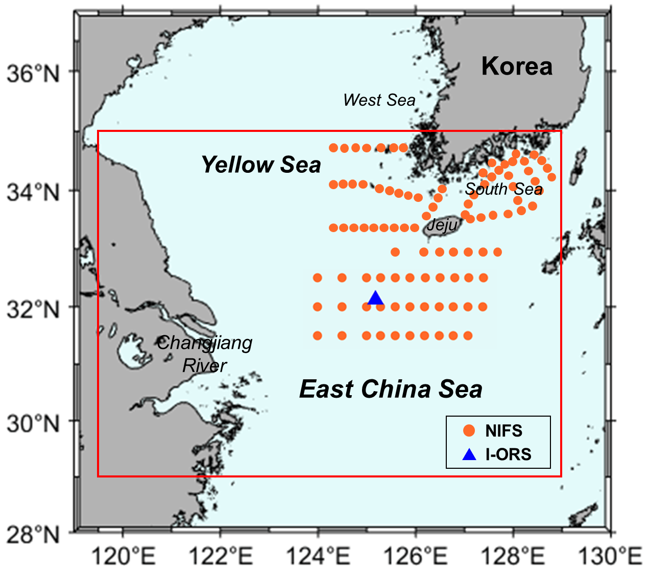
Figure 1The study area in the red solid box (29–35° N, 119.5–129° E) includes the East China Sea (ECS) and Yellow Sea (YS). Orange dots indicate the serial shipboard observation stations from the National Institute of Fisheries Science (NIFS), and the blue triangle indicates the location of the Ieodo Ocean Research Station (I-ORS). The two datasets were used for the model testing.
Table 1Summary of the inputs and output used for training and testing of the machine learning model. The output data were used for the daily SSS map derived from the Geostationary Ocean Color Imager (GOCI) by Kim et al. (2021). In situ SSS data for the model testing were provided by the NIFS and I-ORS.
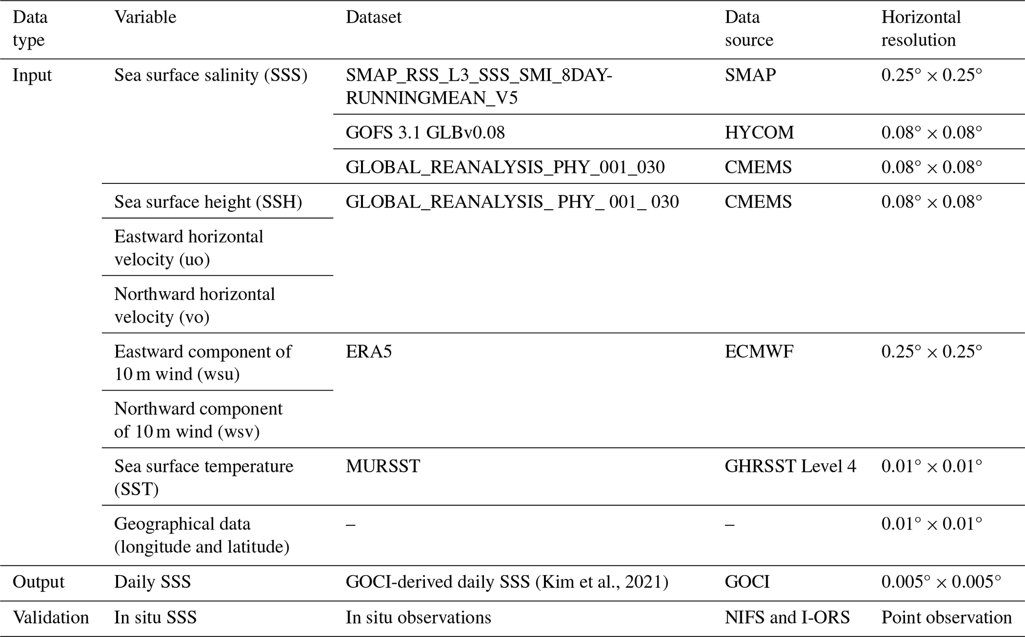
Figure 2 shows a schematic representation of the generation of the gap-free daily SSS product. In this study, we used a daily SSS map at 03:00 UTC during the summer period (June–September) from 2015 to 2019 (610 d) estimated from the GOCI Rrs. We also obtained daily maps of other data for the same period. To match the spatial resolution of the gridded maps, input and output data, as shown in Table 1, were sampled at 0.01°, which is the spatial resolution of the SST level. The SMAP, CMEMS, and HYCOM SSS products were compared with the corresponding GOCI-derived daily SSS map through histograms, spatial distributions, and scatter plots. In addition, the data were divided into below and above 31 psu, which is the standard for identifying the CDW, and each of the two categories was evaluated for consistency with the corresponding GOCI-derived SSS. Thereafter, the machine learning models were trained using a training dataset consisting of pixel pairs of GOCI-derived SSS and various combinations of data, such as environmental factors and geographical data. We evaluated the quantitative performance of each machine learning model using a test dataset. After confirming the performances using in situ SSS, we investigated the time series and spatial SSS distribution of each model. The optimal model was then selected. Finally, we analyzed the CDW front in the ECS as estimated from the selected model. To determine the CDW front, we applied a Savitzky–Golay filter with a window size of four, which smooths according to a quadratic polynomial fitted over each window. This method is more effective when the data vary rapidly. The SSS variations at the location of the I-ORS estimated by the model were compared during the summers of 2015–2019, and the daily progress rate of the CDW was calculated using the time series diagram for the zonal section at the latitude where the I-ORS is located.
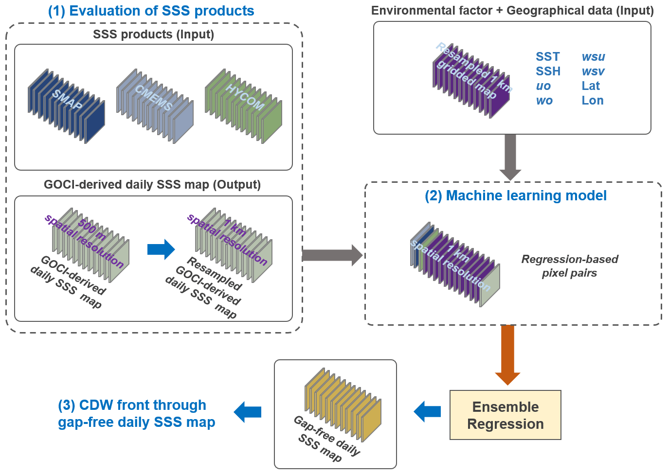
Figure 2Schematic diagram showing the processes that led to the production of the gap-free Geostationary Ocean Color Imager (GOCI)-derived daily sea surface salinity (SSS) map. We performed three steps. (1) We evaluated three SSS products in the ECS, including Soil Moisture Active Passive (SMAP), Copernicus Marine Environment Monitoring Service (CMEMS), and Hybrid Coordinate Ocean Model (HYCOM) SSS with the GOCI-derived SSS data; (2) machine learning models were trained and tested using the GOCI-derived SSS map and various combinations of data, including SSS products and environmental data; and (3) we identified the Changjiang diluted water (CDW) front generated from the gap-free daily SSS map.
3.1 Machine learning models
Machine learning models were trained and tested using various input variable groups. Table 2 summarizes the composition of the input variables, the number of pixel pairs, and the training time for the models. To identify the extent to which the three SSS datasets affected the accuracy of the model, we created seven input variable groups: three input groups (Models 1, 2, and 3) containing only one of the SMAP, CMEMS, and HYCOM SSS products; three input groups (Models 4, 5, and 6) containing combinations of two of the SSS datasets; and one input group containing all three SSS datasets (Model 7). Other data (SST, SSH, uo, vo, wsu, wsv, longitude, and latitude) were included in all the input groups. We matched the pixel pairs between the GOCI-derived daily SSS map and the corresponding factor maps. Because the SMAP SSS does not capture the coast due to its low spatial resolution, the input groups that included it had a small number of matched pixel pairs. In contrast, the input groups containing only the CMEMS and HYCOM SSS products had 500 000 matched pixel pairs or more. For each model, the training and test datasets were 80 % and 20 % of the matched pixel pairs, respectively. Due to differences in spatial resolution between input data, the locations of non-valued pixels differ by input data, so they were adopted as pixel pairs only if all the input values were available. This is because the accuracy of the trained model is degraded if non-valued pixels are included in the input dataset. Then, if at least one of the input data had non-valued pixels, all values of the pixel pairs were converted to zero values. For the training of zero values within the matched images, we added 10 % of the total number of zero matrices for each training and test dataset group. For example, the total number of matched pixel pairs in input group 7 was 425 819, and the numbers of pixel pairs in the training and testing datasets were 340 656 and 85 163, respectively. By adding a zero matrix of 10 % for each pixel pair, the final numbers of pixel pairs for the training and testing datasets were 374 721 and 93 679, respectively. Using the seven input groups, we trained and tested three machine learning models, i.e., the (1) fine trees, (2) boosted trees, and (3) bagged trees models. We used a fine regression tree with a minimum leaf size of four. Regression trees are easy to interpret, are fast for fitting and prediction, and require low memory usage. Boosted trees are an ensemble of regression trees that use a least-squares boosting algorithm. Boosting algorithms use relatively little time or memory compared to bagging but might require more ensemble members. The minimum leaf size was set to eight, and the number of learners was 30 with a learning rate of 0.1 when the boosted trees model was trained. Bagged trees are bootstrap-aggregated ensembles of regression trees. They are often very accurate but can be slow and memory-intensive for large datasets. The minimum leaf size and number of learners in the bagged trees model were the same as those in the boosted trees model. The computational times rank as follows: bagged trees, boosted trees, and fine trees.
Table 2Composition of the input variables, number of pixel pairs, and training time required for each model. The three machine learning models, i.e., the fine trees, boosted trees, and bagged trees models, were trained and tested for estimating SSS from seven input variable groups.

3.2 Performance evaluation
Data comparison was performed using the coefficient of determination (R2), root mean squared error (RMSE), mean squared error (MSE), and mean absolute error (MAE). The MSE is the square of the RMSE. The MAE is always positive and similar to the RMSE but less sensitive to outliers. The formulae are defined as follows:
where N is the number of pairs and i represents an individual pair. x represents the GOCI-derived SSS or in situ observation SSS. y represents the SSS products and the estimated SSS. and are the mean values of x and y, respectively.
4.1 Comparison of the existing SSS with GOCI-derived SSS
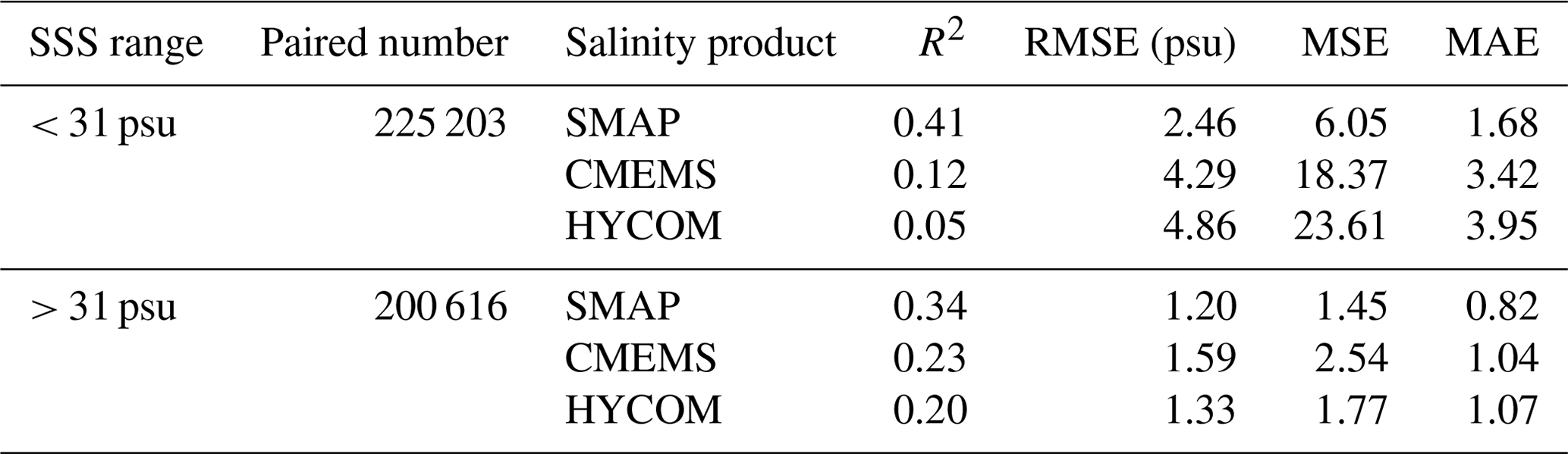
To confirm the characteristics of the SSS products in the study area, we examined the statistical distribution of the SMAP, CMEMS, and HYCOM SSS products against that of the GOCI-derived SSS product (Fig. 3a). The distribution of the SMAP SSS product was most similar to that of the GOCI-derived SSS product, with the median values of the SMAP and GOCI-derived SSS products being 31.04 and 30.86 psu, respectively. However, the SSS ranges of the CMEMS and HYCOM SSS products, especially the one of the latter product, had high probabilities at values close to 35 psu and low probabilities in the range between 25 and 30 psu. For the HYCOM SSS product, there were no values below 20 psu. The median values of the CMEMS and HYCOM SSS products were 32.72 and 33.50 psu, respectively. The HYCOM SSS product showed the lowest degree of agreement with the GOCI-derived SSS product. Figure 3b shows a clear shift of the CDW during summer in the GOCI-derived SSS map on 21 July 2017 at 02:00 UTC, i.e., the date with the least masking (10.25 %) due to cloud cover over the entire study period (610 d). However, we were unable to confirm the movement patterns of the continuous CDW on a daily basis because of cloud masking in most SSS maps within the study period. Figure 3c shows the spatial masking ratio of the GOCI-derived SSS maps with pixel units; the masking ratio was more than 95 % around the Changjiang River estuary. The minimum masking ratio was 72 %, and we estimated that all pixels in the study area could not provide SSS information for at least 439 of the 610 d. Figure 3d–f show the spatial distributions of the SMAP, CMEMS, and HYCOM SSS, respectively, acquired on the day the GOCI-derived SSS map in Fig. 3b was acquired. In addition, we compared the distributions of the SSS data more clearly through scatter plots between the GOCI-derived SSS and the three SSS products (Fig. 3g–i). Consistent with the results in the scatter plot (R2=0.58; RMSE = 1.97 psu), the SMAP SSS map showed the most similar distribution to that of the GOCI-derived SSS map; however, it is an 8 d average product, not a daily product. The CDW pattern in the SMAP SSS was roughly consistent with that of the GOCI-derived SSS; however, in the western waters of Jeju, the CDW pattern in the SMAP SSS did not appear like it did in the GOCI-derived SSS, thereby confirming that the SMAP SSS was slightly overestimated compared with the GOCI-derived SSS in the scatter plot (Fig. 3g). In the case of the CMEMS SSS, the CDW pattern in front of the Changjiang River estuary was similar to that of the GOCI-derived SSS, but the CDW was distributed along the northern coast, and the high SSS area was expanded in the southern waters (Fig. 3e), resulting in a form that deviated significantly from the 1:1 line (R2=0.27; RMSE = 3.34 psu; MSE = 10.91), as shown in Fig. 2h. In contrast, the distribution of the HYCOM SSS had a large expansion of the high SSS area from south to north, and there was no CDW pattern except in the front part of the Changjiang River, which had an extremely low SSS. In line with this, we confirmed that the HYCOM SSS data were considerably overestimated compared to the GOCI-derived SSS data, i.e., R2=0.18 and RMSE = 3.68 psu, especially for the < 31 psu case (Fig. 3i). Through the scatter plots, we confirmed that the degree of agreement differed based on the 31 psu criterion. Table 3 shows the results of calculating the consistency with the corresponding SSS products by dividing the GOCI SSS data based on the 31 psu criterion. Even in the < 31 psu case, the SMAP SSS still showed the best agreement with the GOCI-derived SSS (R2=0.46; RMSE = 2.41 psu), whereas the HYCOM SSS showed the worst agreement (R2=0.05; RMSE = 4.86 psu). However, in the > 31 psu case, the CMEMS and HYCOM SSS products, with RMSE = 1.59 psu for the former and RMSE = 1.33 psu for the latter, showed as much agreement as that of the SMAP SSS with RMSE = 1.20 psu. This was different from the results in the < 31 psu case.
These results may be attributed to the following causes. The characteristics of the reanalysis data may affect the SSS estimation error in the ECS. Jang et al. (2022) compared the SMAP and HYCOM SSS products with in situ data from the global ocean, including the Pacific, tropical, and Arctic oceans, and the Amazon River plume. They reported that the HYCOM SSS in low-salinity regions (< 32 psu), particularly in coastal river-dominated areas, exhibited high uncertainty. This may be because the HYCOM SSS data were assimilated into the ARGO data, which are relatively limited in low-salinity regions. The ARGO database involves few data from our study area – the ECS. The HYCOM model uses SSS climatology and monthly mean river discharge data and does not use satellite-derived SSS products capable of real-time observations. However, these data are too coarse to reproduce the observed rapid changes in low-salinity water in narrow areas (Wallcraft et al., 2009; Cummings and Smedstad, 2014; Wilson and Riser, 2016). Since the CMEMS data are assimilated similarly to HYCOM, it is judged that they have similar limitations of HYCOM data. Therefore, although reanalysis SSS data are gap-free and have a spatial resolution of about 8 km, they are unsuitable for catching daily SSS spatial fluctuations in the waters because it has relatively low accuracy in waters with a low SSS range. Currently, SMAP is the only satellite datum that can provide a continuous spatial SSS distribution in the ECS, although it is an 8 d average dataset and has a rough spatial resolution of 25 km. Hence, the SMAP data have been frequently used as output for SSS estimations using ocean color sensor data. Kim et al. (2021) used the SMAP SSS data as output in an SSS estimation model. The estimated SSS was reasonable, with R2=0.61 and RMSE = 1.08 psu concerning in situ SSS. Because we considered the SSS data produced in Kim's model as output, the SMAP SSS may – naturally – be the most consistent one with the GOCI-derived SSS. Intrinsically, L-band microwave sensor-retrieved SSS has some limitations, such as errors due to anthropogenic RFI and LSC (Olmedo et al., 2019). In addition, the SMAP SSS has significant uncertainty in the polar regions owing to the relatively low SST (Jang et al., 2022). This is because the sensitivity of emissivity to salinity decreases as SST decreases, thereby increasing the error in the SMAP SSS (Dinnat et al., 2019; Reul et al., 2012). In the high-salinity regions, the reanalysis SSS shows a higher association with in situ data than the SMAP SSS. Nevertheless, in the ECS, which has the characteristic of low SSS during summer, the SMAP SSS data are relatively more consistent with the GOCI-derived SSS than the HYCOM and CMEMS data, so they are more suitable for gap-filling of the GOCI SSS data.

Figure 3(a) Histogram of the GOCI-derived, SMAP, CMEMS, and HYCOM SSS products in the study area. Spatial distributions of the (b) GOCI-derived, (d) SMAP, (e) CMEMS, and (f) HYCOM SSS data in the study area. (c) Spatial masking ratio of the GOCI-derived SSS maps based on the pixel unit. Scatter plots showing the consistency patterns between the GOCI-derived SSS and (g) SMAP, (h) CMEMS, and (i) HYCOM SSS data using the entire SSS range. Statistical indices: coefficient of determination (R2), root mean squared error (RMSE), mean squared error (MSE), and mean absolute error (MAE).
Table 3The R2, RMSE, MSE, and MAE for the SMAP, CMEMS, and HYCOM SSS products with respect to the GOCI-derived SSS data according to the SSS range. The SSS data were divided into above and below 31 psu, which is the standard for defining CDW.
4.2 Performance of the SSS models
4.2.1 Quantitative evaluation with the test dataset
Table 4 summarizes the R2, RMSE, MSE, and MAE values of the estimated SSS with respect to the GOCI-derived SSS for the model using the test dataset. Based on the statistical indices, the bagged trees model showed the best results (mean R2=0.977 and RMSE = 1.315 psu), while the boosted trees model had the lowest accuracy (mean R2=0.944 and RMSE = 2.139 psu). The MSE and MAE values suggested the same. The mean MSE and MAE of the boosted trees model were 2.63 and 2.23 times higher than those of the bagged trees model, respectively. The fine trees model performed well, with a mean RMSE of 1.57 psu. Model 1 with the bagged trees model and only the SMAP SSS as input had the highest level (R2=0.98 and RMSE = 1.164 psu). Models 4, 5, and 7 with the bagged trees models and the SMAP SSS as input also had statistical results similar to that of Model 1, with RMSE values of 1.17–1.19 psu. Model 2 with the boosted trees model and only the CMEMS SSS as input showed the worst results (R2=0.93, RMSE = 2.412 psu, MSE = 5.816, and MAE = 1.782). However, the RMSE values were reasonable for the models with the boosted trees model and the SMAP SSS as input (Models 1, 4, 5, and 7). Notably, the RMSE values of Models 2, 3, and 6 with the bagged trees model and without the SMAP SSS as input showed relatively reasonable levels compared to the models that used the SMAP SSS as input. This indicates that the bagged trees model overcomes the inconsistencies of the CMEMS and HYCOM SSS concerning the GOCI-derived SSS compared to the fine trees and boosted trees models.
Our results are similar to those of previous studies. Jang et al. (2022) improved the accuracy of the SMAP SSS for the global ocean using environmental data, the SMAP and HYCOM SSS, and various machine learning approaches. They reported that, among the models, ensemble tree-based machine learning methods such as random forest (RF), extreme gradient boosting (XGBoost), a light gradient boosting (LGB) model, and gradient-boosted regression trees (GBRTs) showed quantitatively good performances. Shin et al. (2022) evaluated machine learning models with various types of ensemble methods, such as bagged trees, boosted trees, subspace discriminant, subspace k-nearest neighbor (KNN), and random undersampling boosting (RUSBoost), to estimate the Sargassum distribution through environmental variables. They found that model accuracy varied depending on the learner type and that the bagged trees model showed the best performance, especially when the learner type was a decision tree. To recognize the impact of geographic factors on model performance, we trained the bagged trees model while excluding the latitude and longitude from the input data of Model 1. As a result, the RMSE, MSE, and MAE values increased by 12.55 %, 26.68 %, and 12.99 %, respectively, compared to those of Model 1 with geographic factors. Spatially, the CDW pattern estimated from the model was more dispersed; therefore, the tendency of the movement pattern was not clear. The results of some previous studies are consistent with these results. Shin et al. (2022) reported that the model trained with geographic factors as input variables was more accurate than the model without geographic factors and that the Sargassum distribution in the ECS estimated from the model was less spread and more reasonable than those from the other models. S. H. Kim et al. (2023) selected physically related variables and geographic factors as inputs to estimate the subsurface salinity using a convolutional neural network (CNN) model. They found that the model without geographic information was less accurate than the model with geographic information. Geographic information is important for the movement of the CDW in the ECS. The Changjiang River, located in the southwestern part of the study area, is a major source of freshwater, and the CDW produced from this location gradually moves northeast. Therefore, a model with a good performance model is possible only when both geographical and environmental factors that can affect the SSS variations are considered.
Table 4Statistical results of the R2, RMSE, MSE, and MAE values between the SSS products estimated from the seven models and the GOCI-derived SSS using the test dataset. The models were divided according to the SSS data used in input, and each training dataset was trained with the three machine learning models, i.e., the fine trees, boosted trees, and bagged trees models.

4.2.2 Validation with independent observations
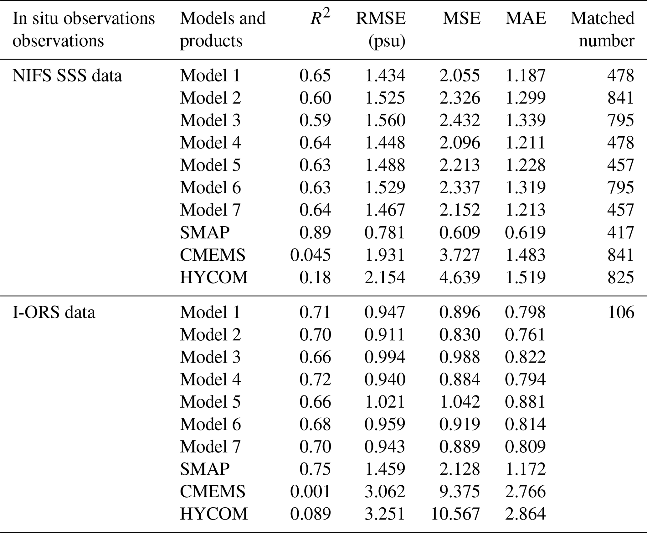
We validated the estimated SSS from the models and the existing SSS products using in situ NIFS and I-ORS SSS (Table 5). Among the models, in the case of in situ NIFS data, Model 1 with the bagged trees model had the best performance with R2=0.65 and RMSE = 1.434 psu, while Model 3 had the worst performance with R2=0.59 and RMSE = 1.560 psu. Consistent with the test dataset results, the models with the SMAP SSS as input (RMSE = 1.434–1.488 psu) performed slightly better than those without the SMAP SSS (RMSE = 1.525–1.560 psu). Among the existing SSS products, the RMSE level of the SMAP was the lowest (0.781 psu), and the CMEMS and HYCOM showed a RMSE of 1.931–2.154 psu. The performance of the models was evaluated using in situ I-ORS data from 2016 when the expansion scale of the CDW was quite large and fast. From June to September 2016, 16 out of 122 d were missing, and 106 matching data points were used to evaluate the performance of the models. Within this period, the minimum SSS was 26.62 psu, and data in the < 31 psu range accounted for 89 % of the total data, with a maximum SSS of 32.02 psu. The RMSE range of all the models was 0.911–1.021 psu, with good performance in a low salinity range. When confirming the consistency between the in situ I-ORS dataset and the three SSS products, the RMSE values of the SMAP, CMEMS, and HYCOM SSS were 1.459, 3.062, and 3.251 psu, respectively. These results were quite different from those when validated using the in situ NIFS data.
Table 5The R2, RMSE, MSE, and MAE values of the SSS values estimated from Models 1–7 for the bagged trees model, SMAP, CMEMS, and HYCOM concerning in situ NIFS and I-ORS SSS data. N is the number of matches between the in situ SSS and estimated SSS maps. As shown in Fig. 1, in situ data were acquired from close to the coast of the Korean Peninsula; therefore, the SMAP SSS does not provide data around the coast. For this reason, the SSS map estimated from models using the SMAP SSS as input had fewer matched data than those of other models. Since I-ORS is located in the center of the study area, in situ data that matched data on the SSS map estimated from models were the same for all the models. Of the 122 d, 16 d were missing, and a total of 106 d were matched.
We evaluated model performance by dividing the data based on the 31 psu criterion using in situ NIFS SSS data (Table 6). As shown in Fig. 1, in situ NIFS data were acquired from within the area of the CDW, with a minimum SSS of 21.97 psu. Quite a few data were acquired from the northern location, unaffected by the CDW; therefore, the maximum SSS was 34.04 psu. However, of the 861 in situ data, the ones in the > 31 psu range accounted for 73.17 % of the total, unlike the in situ I-ORS data. When using in situ data in the > 31 psu range, the mean RMSE (1.573 psu) was 5.36 % higher than the mean RMSE of the entire dataset (1.493 psu), and the performances of all the models were slightly worse. However, when in situ data in the < 31 psu range were used, the mean RMSE (1.308 psu) decreased by 12.32 % compared to the mean RMSE of the entire dataset. In particular, the RMSE (1.301 psu) of Model 2 (with only the CMEMS SSS as input) decreased by 14.68 % compared with when all the data were used (1.525 psu). The model performance with data in the < 31 psu range was similarly reasonable in all seven models (RMSE = 1.250–1.347 psu). Our models successfully solved the nonlinear relationships between the input dataset and the GOCI-derived SSS data. This indicates that, in a water environment with a low salinity range, the SSS data estimated by our models have a higher accuracy than the existing SSS products, approximately the accuracy level of RMSE = 1 psu.
Table 6The R2, RMSE, MSE, and MAE values between the SSS values estimated from Models 1–7 for the bagged trees model and in situ NIFS SSS data. The data were evaluated by dividing according to a 31 psu criterion.

4.2.3 Time series and spatial distribution of the SSS map
We compared the spatial distributions of the SSS maps to qualitatively evaluate the models. Figure 4 shows the time series variations of the model-based SSS, GOCI-derived SSS, and in situ I-ORS SSS during the summer period, i.e., from 1 June to 30 September 2016. Out of a total of 122 d, GOCI-derived SSS data were obtained at the I-ORS location in 48 d, while 60.66 % of the SSS data over 4 months were not observable due to cloud cover. The in situ I-ORS data were missing 13.11 % during the same period. However, the SSS data estimated by the models spanned over the entire period and did not include missing data, and the simulated daily variation of the in situ data was better than that of the GOCI-derived SSS. Figure 5a shows the GOCI-derived SSS map on 27 July 2016, in which the in situ I-ORS SSS value is the lowest, as shown in Fig. 4. SSS data at the location of the I-ORS (red triangle) existed in the GOCI-derived SSS map; however, most parts of the study area were masked by clouds, making it difficult to recognize the CDW pattern. In contrast, Fig. 5b–h show the SSS maps estimated by Models 1–7, respectively, for the same date as that of the GOCI-derived SSS map. Unlike the GOCI-derived SSS map, all the SSS maps estimated by the models provided gap-free SSS distributions and clearly showed that the CDW extended from the Changjiang River estuary to the coast of Jeju during summer. However, we confirmed that Models 1, 4, 5, and 7 (Fig. 5b, e, f, and h, respectively), which included the SMAP SSS as input, are masked in coastal areas, and some of the spatial patterns of the CDW appear in steps because of the spatial resolution of the SMAP (25 km). In contrast, Models 2, 3, and 6 (Fig. 5c, d, and g, respectively), which included the CMEMS and HYCOM SSS as inputs, did not mask the coastal area and provided coastal SSS information regarding the CDW spreading from the front of the Changjiang River estuary. Overall, the CDW patterns in the SSS maps estimated by Models 3 and 6 (Fig. 5d and g) using the HYCOM SSS as input data were similar to those of the other models; however, the CDW distribution tended to be divided around 124° E. Model 2, which only included the CMEMS SSS as input, showed the appropriate CDW distributions and patterns. Through quantitative and qualitative evaluation of the models, we selected Model 1 (only the SMAP SSS as input) and Model 2 (only the CMEMS SSS as input) for the CDW front analysis in the ECS while considering the simplicity of the input data. The prime SMAP mission was completed in the summer of 2018, having acquired a wide range of scientific data for 3 years. Since then, SMAP has been approved for an extended phase of operation until 2023. However, the SMAP operation will soon be terminated; therefore, an alternative to the SMAP SSS data is necessary. By quantitative and qualitative model evaluation using a combination of SSS products, we confirmed the usefulness of additional CMEMS SSS data, combined with the SMAP SSS data, for generating a gap-free GOCI-derived SSS map.

Figure 4(a) SSS time series estimated from seven models with bagged trees and the GOCI-derived and in situ I-ORS SSS data over 122 d from 1 June to 30 September 2016.

Figure 5(a) GOCI-derived SSS map on 27 July 2016. (b–h) SSS maps estimated from seven models with bagged trees. The estimated SSS maps were generated from input data on the same day as the GOCI-derived SSS map. The red triangle represents the I-ORS location.
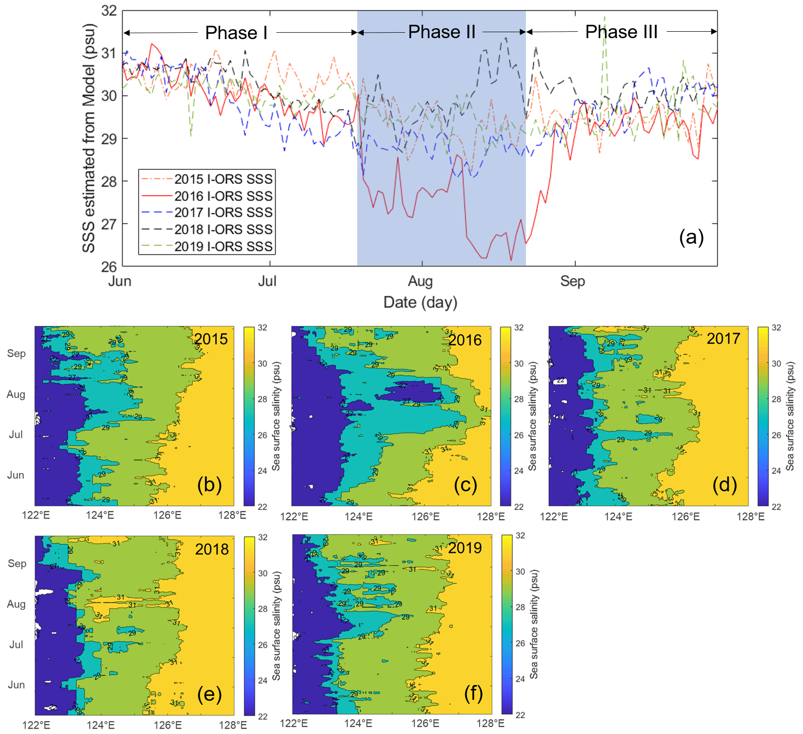
Figure 6(a) SSS time series estimated by Model 1 (2015, 2016, 2017, and 2018) and Model 2 (2019) with bagged trees at the I-ORS location during the summer of 2015–2019. (Phase I) Beginning phase, (Phase II) development phase, and (Phase III) recovery phase of the CDW. In 2019, it was not possible to estimate the SSS with Model 1 because the SMAP SSS was not provided due to safe mode; therefore, Model 2 was used instead. (b–f) Time series of the 122–128° E horizontal transect (A–A′ in Fig. 8a) during summer in each year. The plots were applied for the 27, 29, and 31 psu isohalines. The cross section in A–A′ is located at 32.12° N.
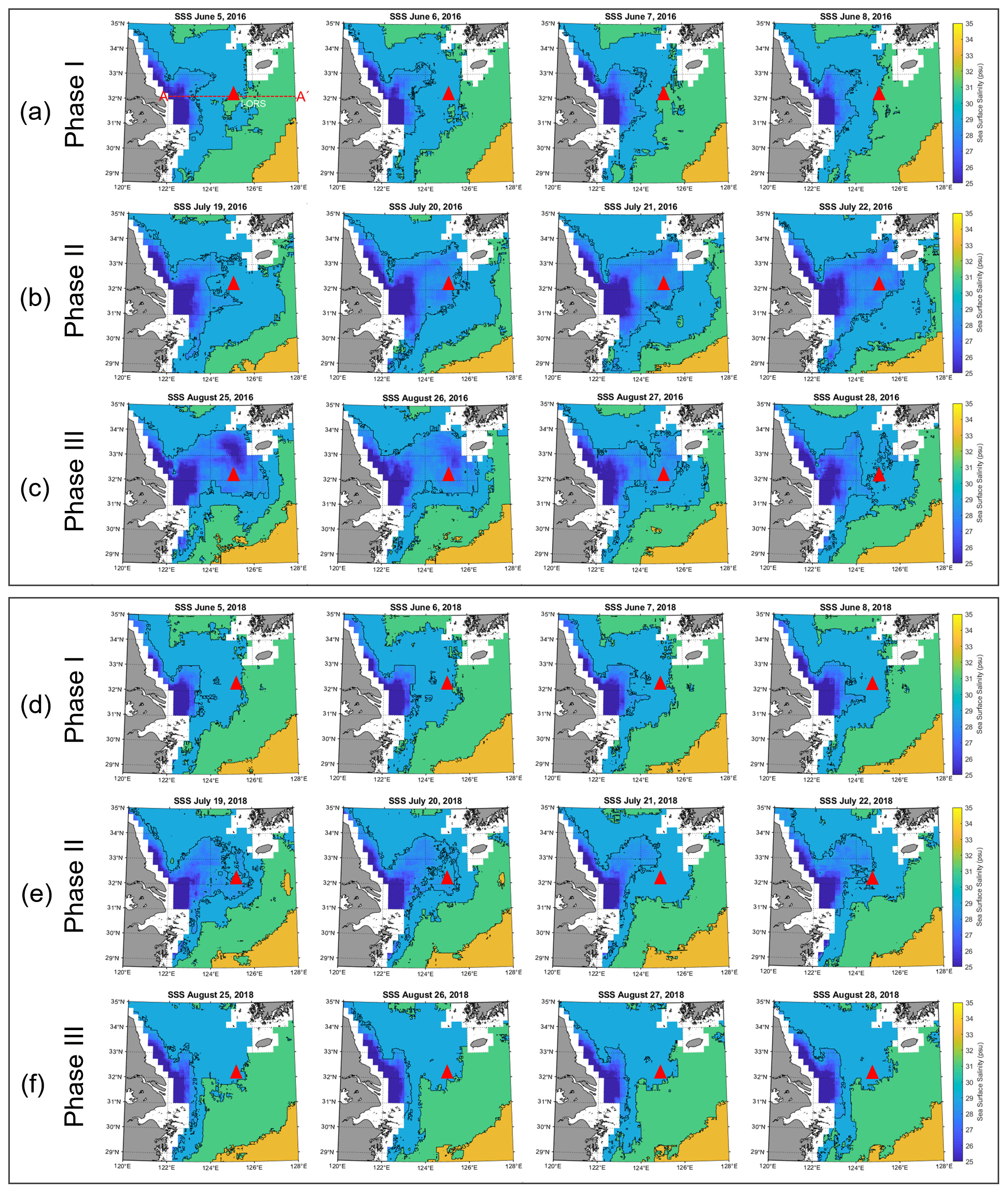
Figure 7SSS spatial distribution in the ECS with the 29, 31, and 33 psu isohalines in 2016 and 2018. (a–f) Maps corresponding to the stages in panels (a), (b), and (c), respectively. Beginning phase (Phase I): panels (a) and (c); development phase (Phase II): panels (b) and (d); recovery stage (Phase III): panels (c) and (f). The red triangle represents the I-ORS location (32.12° N, 125.18° E).
4.3 CDW front based on gap-free daily SSS
Figure 6a shows the SSS time series estimated from Models 1 (2015, 2016, 2017, and 2018) and 2 (2019) with bagged trees at the I-ORS location during the summers of 2015–2019. The estimated SSS data with Model 1 in 2019 were not possible because the SMAP SSS was not provided due to safe mode; therefore, Model 2 was used instead. We identified the three phases according to the CDW variations during summer: (Phase I) beginning phase (early June), (Phase II) development phase (end of July), and (Phase III) recovery phase (end of August). The in situ I-ORS SSS generally began to fall under the influence of the CDW in June (Phase I), declined from July to August (Phase II), and then increased in September (Phase III). This happened in 2015, 2016, and 2019, and the difference between the maximum and minimum SSS was approximately 3 psu. However, 2016 and 2018 exhibited different trends. In 2016, the SSS change in Phase I was similar to those in other years, whereas Phase II showed a sharp SSS decline, in contrast to the cases in the other years. At the end of August, Phase III showed a sharp SSS increase and SSS recovered to a level similar to those in other years. In contrast, in 2018, Phases I and III showed patterns similar to those in other years, whereas Phase II showed a slight SSS increase, in contrast to the case in 2016. To determine the direction and velocity of the CDW front movement in the summers of 2015–2019, we plotted the time series in the cross-sectional direction (A–A′ in Fig. 7a). In early June, the CDW front was similarly located near 126° E in all the years, and the 29 isohaline appeared near 124° E. In 2015 and 2019, the CDW front expanded to 127° E and gradually moved east until September. In 2017 and 2018, the CDW front did not reach 127° E until September, repeating the trend of heading east and retreating to the west. In an unusual case in 2016, we confirmed that the CDW front extended to 128° E on 1 August, 62 d after 1 June, moving approximately 3.04 km d−1 (188.29 km/62 d). Regarding the 29 isohaline, in 2017 and 2018, similar to June, it rarely moved east; in particular, in 2018, the tendency to move east was low, resulting in the lowest CDW expansion during the study period. In 2015 and 2019, the 29 isohaline developed at 125° E in August and gradually retreated westward. In 2016, the 29 isohaline extended to 127° E from early June to early August, moving at approximately 4.79 km d−1 (282.42 km/59 d). This was faster than the CDW front, which lasted 1 month in August and then gradually retreated in September. The 27 isohaline stayed around 123° E from early June to the end of September in all the years except 2016. In 2016, a partial 27 isohaline extended to 126° E, confirming that a fairly low-salinity environment persisted during the summer season of 2016.
Focusing on 2016 and 2018, which showed unusual SSS fluctuations different from those in the other years, we continuously (i.e., on a daily basis) identified the CDW front (< 31 psu) by phase (Fig. 7). The SSS spatial distributions were estimated by Model 1 and were applied with the 29, 31, and 33 psu isohalines for the CDW front. Consistent with the SSS time series in Fig. 6, the CDW front was close to the I-ORS during Phase I in early June (5–8 June) in both 2016 and 2018 (Fig. 7a and d, respectively). This indicates that, before June, the CDW front had already advanced considerably eastward in the ECS and began to enter the CDW boundary of the < 31 psu range in Phase I. However, the CDW front variation patterns in Phases II and III differed. On 19–20 July 2016, during Phase I, the I-ORS location entered the 29 psu boundary, and the CDW front gradually expanded southeast. Conversely, in 2018, Phase I stayed at the 29 psu boundary simultaneously and escaped, and the CDW front remained similar without significant changes. While Phase III in 2016 remained at the 29 psu boundary and gradually escaped, Phase III in 2018 exhibited a spatial CDW front pattern similar to that of Phase I, and the SSS level had already recovered.
Our results are consistent with those of previous studies on the CDW in the ECS. Moon et al. (2019) recognized that ocean salinity in 2016 was exceptionally low and investigated the contribution of low salinity to sea surface warming in the ECS during the summer of 2016. Through observations, they revealed that a large amount of freshwater in 2016 originated from the Changjiang River. Son and Choi (2022) presented maps that applied various SSS algorithms to GOCI and noted that surface water in the summer of 2016 was loaded with freshwater owing to increased CRD. In addition, cross- and along-shelf exports of the CDW from the Changjiang River mouth manifested as patches, and salinities below 25 psu were observed along the Changjiang River estuary. S. H. Kim et al. (2023) estimated the CDW volume in the ECS by combining a subsurface salinity map with the SMAP SSS. The CDW volume was highest in 2016, whereas in 2018 it reached a minimum during summer. They found that the CDW volumes were relatively low from May to early June and increased from June to August, showing a seasonal trend. This may be because the conditions in 2016 and 2018 were different, owing to the amount of CRD, precipitation, El Niño–Southern Oscillation (ENSO), typhoons, and wind. The primary factor controlling the scale of the CDW is the amount of CRD. S. H. Kim et al. (2023) reported that the amount of CRD measured at the Datong station was highest in 2016 and lowest in 2018. They investigated the relationship between CDW volume and CRD and found that the CDW volume peak appeared with a time lag of about 34 ± 15 d after an increase in CRD, that 2016 had the largest CDW, and that 2018 had the smallest CDW. In 2016, a strong El Niño event led to a noticeable increase in CRD compared to the other years (S. H. Kim et al., 2023). ENSO can increase the CRD in the ECS through the increased precipitation during El Niño events (Park et al., 2011; Wu et al., 2023). In addition, no typhoons crossed the ECS in 2016, indicating that no vertical mixing was caused by typhoons. Strong vertical mixing caused by the passage of a typhoon hinders the CDW expansion. In contrast, the La Niña event in 2018 led to a low CRD and typhoons crossed the ECS. These differences may change the CDW pattern annually.
The gridded gap-free SSS dataset at 0.01° × 0.01° spatial resolution during the summer period (June–September) from 2015 to 2019 is stored at the Korea Institute of Ocean Science and Technology – KOIST (https://doi.org/10.22808/DATA-2023-2, Shin et al., 2023). When analyzing the CDW front, Model 1 was used from 2015 to 2018 and Model 2 was used for 2019 due to the safe mode of SMAP SSS data. We provided the SSS dataset of Models 1 and 2 from 2015 to 2019.
To date, the SMAP satellite data and CMEMS and HYCOM reanalysis data are the gap-free gridded SSS products that can be used in the ECS. The reanalysis data showed fair accuracy with respect to the GOCI-derived SSS in the > 31 psu range, while the worst agreement was found in the < 31 psu range in the ECS during the summer seasons. Hence, the reanalysis SSS data were unsuitable for gap-filling in the GOCI-derived SSS. Because the SMAP SSS dataset is an 8 d average dataset, the accuracy of the daily analysis was poor and had a fairly rough spatial resolution of 25 km; however, to date, it is the only dataset that can grasp the gap-free daily spatial SSS distribution with fair accuracy in the < 31 psu range. The spatial resolution of these data may be too rough to capture the daily variations of the CDW moving 12–17 km d−1. In this study, we overcame the limitations of these datasets and succeeded in producing a gap-free gridded daily SSS product with reasonable accuracy and a spatial resolution of 1 km using a machine learning approach and the corresponding variable of SSS estimation. Eventually, the data produced from our study enabled the recognition of SSS distribution and movement patterns of the CDW front in the ECS daily during summer, which were not previously attempted due to spatial and temporal resolution limitations. These results will further advance our understanding and monitoring of long-term SSS variations in the ECS.
JS developed the related model and evaluated and wrote the manuscript. YH conceptualized and supervised this study. DW and SH participated in data processing. YH, BK, and SH revised and reviewed the manuscript.
The contact author has declared that none of the authors has any competing interests.
Publisher’s note: Copernicus Publications remains neutral with regard to jurisdictional claims made in the text, published maps, institutional affiliations, or any other geographical representation in this paper. While Copernicus Publications makes every effort to include appropriate place names, the final responsibility lies with the authors.
The serial oceanographic observation and I-ORS data were provided by the NIFS and the KOIST, respectively. The authors would like to thank the staff of the data management.
This work was supported by the National Research Foundation of Korea (NRF) and the Korean government (MSIT) (grant nos. RS-2023-00280650 and RS-2023-00274972).
This paper was edited by Alberto Ribotti and reviewed by two anonymous referees.
Bagnell, A. and DeVries, T.: 20th century cooling of the deep ocean contributed to delayed acceleration of Earth's energy imbalance, Nat. Commun., 12, 4604, https://doi.org/10.1038/s41467-021-24472-3, 2021.
Balmaseda, M. A., Trenberth, K. E., and Källén, E.: Distinctive climate signals in reanalysis of global ocean heat content, Geophys. Res. Lett., 40, 1754–1759, https://doi.org/10.1002/grl.50382, 2013.
Beardslev, R. C., Limeburner, R., Yu, H., and Cannon, G. A.: Discharge of the changjiang (Yangtze river) into the East China Sea, Cont. Shelf. Res., 4, 57–76, https://doi.org/10.1016/0278-4343(85)90022-6, 1985.
Chang, P. H. and Isobe, A.: A numerical study on the changjiang diluted water in the yellow and East China seas, J. Geophys. Res., 108, 3299, https://doi.org/10.1029/2002JC001749, 2003.
Chen, C., Xue, P., Ding, P., Beardsley, R. C., Xu, Q., Mao, X., Gao, G., Qi, J., Li, C., Lin, H., Cowles, G., and Shi, M.: Physical mechanisms for the offshore detachment of the Changjiang Diluted Water in the East China Sea, J. Geophys. Res.-Oceans, 113, C02002, https://doi.org/10.1029/2006JC003994, 2008.
Chen, S. and Hu, C.: Estimating Sea Surface Salinity in the Northern Gulf of Mexico from Satellite Ocean Color Measurements, Remote Sens. Environ., 201, 115–132, https://doi.org/10.1016/j.rse.2017.09.004, 2017.
Cheng, L., Trenberth, K. E., Gruber, N., Abraham, J. P., Fasullo, J. T., Li, G., Mann, M. E., Zhao, X., and Zhu, J.: Improved estimates of changes in upper ocean salinity and the hydrological cycle, J. Climate, 33, 10357–10381, https://doi.org/10.1175/JCLI-D-20-0366.1, 2020.
Cheng, L. and Zhu, J.: Benefits of CMIP5 multimodel ensemble in reconstructing historical ocean subsurface temperature variations, J. Climate, 29, 5393–5416, https://doi.org/10.1175/JCLI-D-15-0730.1, 2016.
Choi, J. K., Son, Y. B., Park, M. S., Hwang, D. J., Ahn, J. H., and Park, Y. G.: The Applicability of the Geostationary Ocean Color Imager to the Mapping of Sea Surface Salinity in the East China Sea, Remote Sens., 13, 2676, https://doi.org/10.3390/rs13142676, 2021.
Ciais, P., Sabine, C., Bala, G., Bopp, L., Brovkin, V., Canadell, J., Chhabra, A., DeFries, R., Galloway, J., Heimann, M., Jones, C., Quéré, C. Le, Myneni, R. B., Piao, S., and Thornton, P.: The physical science basis. Contribution of working group I to the fifth assessment report of the intergovernmental panel on climate change, Chang. IPCC Clim., https://doi.org/10.1017/CBO9781107415324.015, 2013.
Cummings, J. A. and Smedstad, O. M.: Ocean data impacts in global HYCOM, J. Atmos. Ocean. Tech., 31, 1771–1791, https://doi.org/10.1175/JTECH-D-14-00011.1, 2014.
Dinnat, E. P., Le Vine, D. M., Boutin, J., Meissner, T., and Lagerloef, G.: Remote Sensing of Sea Surface Salinity: Comparison of Satellite and in situ Observations and Impact of Retrieval Parameters, Remote Sens., 11, 750, https://doi.org/10.3390/rs11070750, 2019.
Domingues, C. M., Church, J. A., White, N. J., Gleckler, P. J., Wijffels, S. E., Barker, P. M., and Dunn, J. R.: Improved estimates of upper-ocean warming and multi-decadal sea-level rise, Nature, 453, 1090–1093, https://doi.org/10.1038/nature07080, 2008.
Durack, P. J., Lee, T., Vinogradova, N. T., and Stammer, D.: Keeping the Lights on for Global Ocean Salinity Observation, Nat. Clim. Chang., 6, 228, https://doi.org/10.1038/nclimate2946, 2016.
Forget, G., Campin, J.-M., Heimbach, P., Hill, C. N., Ponte, R. M., and Wunsch, C.: ECCO version 4: an integrated framework for non-linear inverse modeling and global ocean state estimation, Geosci. Model Dev., 8, 3071–3104, https://doi.org/10.5194/gmd-8-3071-2015, 2015.
Geiger, E. F., Grossi, M. D., Trembanis, A. C., Kohut, J. T., and Oliver, M. J.: Satellite-Derived Coastal Ocean and Estuarine Salinity in the Mid-Atlantic, Cont. Shelf Res., 63, S235–242, https://doi.org/10.1016/j.csr.2011.12.001, 2013.
Jang, E., Kim, Y. J., Im, J., and Park, Y. G.: Improvement of SMAP sea surface salinity in river-dominated oceans using machine learning approaches, GIsci. Remote Sens., 58, 138–160, https://doi.org/10.1080/15481603.2021.1872228, 2021.
Jang, E., Kim, Y. J., Im, J., Park, Y. G., and Sung, T.: Global Sea Surface Salinity via the Synergistic Use of SMAP Satellite and HYCOM Data Based on Machine Learning, Remote Sens. Environ., 273, 112980, https://doi.org/10.1016/j.rse.2022.112980, 2022.
Kim, D. W., Park, Y. J., Jeong, J. Y., and Jo, Y. H.: Estimation of Hourly Sea Surface Salinity in the East China Sea Using Geostationary Ocean Color Imager Measurements, Remote Sens., 12, 755, https://doi.org/10.3390/rs12050755, 2020.
Kim, D. W., Kim, S. H., and Jo, Y. H.: A development for Sea Surface Salinity Algorithm Using GOCI in the East China Sea, Korean J. Remote Sens., 37, 1307–1315, https://doi.org/10.7780/kjrs.2021.37.5.2.8, 2021.
Kim, D. W., Kim, S. H., Baek, J. Y., Lee, J. S., and Jo, Y. H.: GOCI-II based sea surface salinity estimation using machine learning for the first-year summer, Int. J. Remote Sens., 43, 6605–6623, https://doi.org/10.1080/01431161.2022.2142080, 2022a.
Kim, D. W., Kim, S. H., and Jo, Y. H.: Machine Learning to Identify Three Types of Oceanic Fronts Associated with the Changjiang Diluted Water in the East China Sea between 1997 and 2021, Remote Sens., 14, 3574, https://doi.org/10.3390/rs14153574, 2022b.
Kim, H. C., Yamaguchi, H., Yoo, S., Zhu, J., Okamura, K., Kiyomoto, Y., Tanaka, K., Kim, S. W., Park, T., and Ishizaka, J.: Distribution of Changjiang diluted water detected by satellite chlorophyll-a and its interannual variation during 1998–2007, J. Oceanogr., 65, 129–135, https://doi.org/10.1007/s10872-009-0013-0, 2009.
Kim, S. H., Shin, J., Kim, D. W., and Jo, Y. H.: Estimation of subsurface salinity and analysis of Changjiang diluted water volume in the East China Sea, Front. Mar. Sci., 10, 1247462, https://doi.org/10.3389/fmars.2023.1247462, 2023.
Kim, Y. J., Han, D., Jang, E., Im, J., and Sung, T.: Remote sensing of sea surface salinity: challenges and research directions, GIsci. Remote Sens., 60, 2166377, https://doi.org/10.1080/15481603.2023.2166377, 2023.
Lie, H. J., Cho, C. H., Lee, J. H., and Lee, S.: Structure and eastward extension of the Changjiang River plume in the East China Sea, J. Geophys. Res.-Oceans, 108, 3077, https://doi.org/10.1029/2001JC001194, 2003.
Liu, R., Zhang, J., Yao, H., Cui, T., Wang, N., Zhang, Y., Wu, L., and An, J.: Hourly Changes in Sea Surface Salinity in Coastal Waters Recorded by Geostationary Ocean Color Imager, Estuar. Coast. Shelf S., 196, 227–236, https://doi.org/10.1016/j.ecss.2017.07.004, 2017.
Lu, S., Liu, Z., Li, H., Li, Z., and Xu, J.: Manual of Global Ocean Argo gridded data set (BOA_Argo) (Version 2020), SOED & DESS, Hangzhou, China, 14 pp., 2020.
Lyman, J. M. and Johnson, G. C.: Estimating global ocean heat content changes in the upper 1800 m since 1950 and the influence of climatology choice, J. Climate, 27, 1945–1957, https://doi.org/10.1175/JCLI-D-12-00752.1, 2014.
Moon, J. H., Kim, T., Son, Y. B., Hong, J. S., Lee, J. H., Chang, P. H., and Kim, S. K.: Contribution of low-salinity water to sea surface warming of the East China Sea in the summer of 2016, Prog. Oceanogr., 175, 68–80, https://doi.org/10.1016/j.pocean.2019.03.012, 2019.
Olmedo, E., Taupier-Letage, I., Turiel, A., and Alvera-Azcaìrate, A.: Improving SMOS sea surface salinity in the Western Mediterranean sea through multivariate and multifractal analysis, Remote Sens., 10, 485, https://doi.org/10.3390/rs10030485, 2018.
Olmedo, E., González-Gambau, V., Turiel, A., Martínez, J., Gabarró, C., Portabella, M., Ballabrera-Poy, J., Arias, M., Sabia, R., and Oliva, R.: Empirical characterization of the SMOS brightness temperature bias and uncertainty for improving sea surface salinity retrieval, IEEE J. Sel. Top. Appl. Earth Obs., 12, 2486–2503, https://doi.org/10.1109/JSTARS.2019.2904947, 2019.
Palmer, M. D., Roberts, C. D., Balmaseda, M., Chang, Y. S., Chepurin, G., Ferry, N., Fujii, Y., Good, S. A., Guinehut, S., Haines, K., Hernandez, F., Köhl, A., Lee, T., Martin, M. J., Masina, S., Masuda, S., Peterson, K. A., Storto, A., Toyoda, T., Valdivieso, M., Vernieres, G., Wang, O., and Xue, Y.: Ocean heat content variability and change in an ensemble of ocean reanalyses, Clim. Dynam., 49, 909–930, https://doi.org/10.1007/s00382-015-2801-0, 2017.
Park, T., Jang, C. J., Jungclaus, J. H., Haak, H., and Park, W.: Effects of the Changjiang river discharge on sea surface warming in the Yellow and East China Seas in summer, Cont. Shelf Res., 31, 15–22, https://doi.org/10.1016/j.csr.2010.10.012, 2011.
Reul, N., Tenerelli, J., Boutin, J., Chapron, B., Paul, F., Brion, E., Gaillard, F., and Archer, O.: Overview of the first SMOS sea surface salinity products. Part I: quality assessment for the second half of 2010, IEEE T. Geosci. Remote Sens., 50, 1636–1647, https://doi.org/10.1109/TGRS.2012.2188408, 2012.
Reul, N., Grodsky, S. A., Arias, M., Boutin, J., Catany, R., Chapron, B., D'Amico, F., Dinnat, E., Donlon, C., Fore, A., Fournier, S., Guimbard, S., Hasson, A., Kolodziejczyk, N., Lagerloef, G., Lee, T., Le Vine, D. M., Lindstrom, E., Maes, C., Mecklenburg, S., Meissner, T., Olmedo, E., Sabia, R., Tenerelli, J., Thouvenin-Masson, C., Turiel, A., Vergely, J. L., Vinogradova, N., Wentz, F., and Yueh, S.: Sea Surface Salinity Estimates from Spaceborne L-Band Radiometers: An Overview of the First Decade of Observation 2010–2019, Remote Sens. Environ., 242, 111769, https://doi.org/10.1016/j.rse.2020.111769, 2020.
Roemmich, D. and Gilson, J.: The 2004–2008 mean and annual cycle of temperature, salinity, and steric height in the global ocean from the Argo Program, Prog. Oceanogr., 82, 81–100, https://doi.org/10.1016/j.pocean.2009.03.004, 2009.
Shin, J., Choi, J. G., Kim, S. H., Khim, B. K., and Jo, Y. H.: Environmental variables affecting Sargassum distribution in the East China Sea and the Yellow Sea, Front. Mar. Sci., 9, 1055339, https://doi.org/10.3389/fmars.2022.1055339, 2022.
Shin, J., Kim, D. W., Kim, S. H., Kim, G. S., Khim, B. K., and Jo, Y. H.: Gap-free daily sea surface salinity product in the East China Sea during summer in 2015–2019, ScienceWatch@KIOST [data set], https://doi.org/10.22808/DATA-2023-2, 2023.
Son, Y. B. and Choi, J. K.: Mapping the Changjiang diluted water in the East China Sea during summer over a 10-year period using GOCI satellite sensor data, Front. Mar. Sci., 9, 1024306, https://doi.org/10.3389/fmars.2022.1024306, 2022.
Storto, A., Alvera-Azcárate, A., Balmaseda, M. A., Barth, A., Chevallier, M., Counillon, F., Domingues, C. M., Drévillon, M., Vinogradova, N., Lee, T., Boutin, J., Drushka, K., Fournier, S., Sabia, R., Stammer, D., Bayler, E., Reul, N., Gordon, A., Melnichenko, O., Li, L., Hackert, E., Martin, M., Kolodziejczyk, N., Hasson, A., Brown, S., Misra, S., and Lindstrom, E.: Satellite salinity observing system: Recent discoveries and the way forward, Front. Mar. Sci., 6, 243, https://doi.org/10.3389/fmars.2019.00243, 2019.
Sun, D., Su, X., Qiu, Z., Wang, S., Mao, Z., and He, Y.: Remote Sensing Estimation of Sea Surface Salinity from GOCI Measurements in the Southern Yellow Sea, Remote Sens., 11, 775, https://doi.org/10.3390/rs11070775, 2019.
Trenberth, K. E., Large, W. G., and Olson, J. G.: The mean annual cycle in global ocean wind stress, J. Phys. Oceanogr., 20, 1742–1760, https://doi.org/10.1175/1520-0485(1990)020<1742:TMACIG>2.0.CO;2, 1990.
Vinogradova, N., Lee, T., Boutin, J., Drushka, K., Fournier, S., Sabia, R., Stammer, D., Bayler, E., Reul, N., Gordon, A., Melnichenko, O., Li, L., Hackert, E., Martin, M., Kolodziejczyk, N., Hasson, A., Brown, S., Misra, S., and Lindstrom, E.: Satellite salinity observing system: Recent discoveries and the way forward, Front. Mar. Sci., 6, 428925, https://doi.org/10.3389/fmars.2019.00243, 2019.
von Schuckmann, K., Sallée, J.-B., Chambers, D., Le Traon, P.-Y., Cabanes, C., Gaillard, F., Speich, S., and Hamon, M.: Consistency of the current global ocean observing systems from an Argo perspective, Ocean Sci., 10, 547–557, https://doi.org/10.5194/os-10-547-2014, 2014.
Wallcraft, A. J., Metzger, E. J., and Carroll, S. N.: Software design description for the hybrid coordinate ocean model (HYCOM), Version 2.2. Naval Research Lab Stennis Space Center Ms Oceanography Div., 2009.
Wang, J. and Deng, Z.: Development of a MODIS Data Based Algorithm for Retrieving Nearshore Sea Surface Salinity Along the Northern Gulf of Mexico Coast, Int. J. Remote Sens., 39, 3497–3511, https://doi.org/10.1080/01431161.2018.1445880, 2018.
Wilson, E. A. and Riser, S. C.: An assessment of the seasonal salinity budget for the upper Bay of Bengal, J. Phys. Oceanogr., 46, 1361–1376, https://doi.org/10.1175/JPO-D-15-0147.1, 2016.
Wu, Q., Wang, X., He, Y., and Zheng, J.: The Relationship between Chlorophyll Concentration and ENSO Events and Possible Mechanisms off the Changjiang River Estuary, Remote Sens., 15, 2384, https://doi.org/10.3390/rs15092384, 2023.
Yamaguchi, H., Kim, H. C., Son, Y. B., Kim, S. W., Okamura, K., Kiyomoto, Y., and Ishizaka, J.: Seasonal and summer interannual variations of SeaWiFS chlorophyll a in the Yellow Sea and East China Sea, Prog. Oceanogr., 105, 22–29, https://doi.org/10.1016/j.pocean.2012.04.004, 2012.
Zhou, G., Fu, W., Zhu, J., and Wang, H.: The impact of location-dependent correlation scales in ocean data assimilation, Geophys. Res. Lett., 31, L21306, https://doi.org/10.1029/2004GL020579, 2004.