Mapping 24 woody plant species phenology and ground forest phenology over China from 1951 to 2020

Plant phenology refers to cyclic plant growth events, and is one of the most important indicators of climate change. Integration of plant phenology information is crucial for understanding the ecosystem response to global change and modeling the material and energy balance of terrestrial ecosystems. Utilizing 24 552 in situ phenological observations of 24 representative woody plant species from the Chinese Phenology Observation Network (CPON), we have developed maps delineating species phenology (SP) and ground phenology (GP) of forests over China from 1951 to 2020. These maps offer a detailed spatial resolution of 0.1° and a temporal resolution of 1 d. Our method involves a model-based approach to upscale in situ phenological observations to SP maps, followed by the application of weighted average and quantile methods to derive GP maps from the SP data. The resulting SP maps for the 24 woody plants exhibit a high degree of concordance with in situ observations, manifesting an average deviation of 6.9 d for spring and 10.8 d for autumn phenological events. Moreover, the GP maps demonstrate robust alignment with extant land surface phenology (LSP) products sourced from remote sensing data, particularly within deciduous forests, where the average discrepancy is 8.8 d in spring and 15.1 d in autumn. This dataset provides an independent and reliable phenology data source for China on a long-time scale of 70 years, and contributes to more comprehensive research on plant phenology and climate change at both regional and national scales. The dataset can be accessed at https://doi.org/10.57760/sciencedb.07995 (Zhu and Dai, 2023).

1 Introduction

Plant phenology, the discipline that examines the timing of plant life cycle events, is emerging in response to the seasonal changes in climate and environmental conditions (Lieth, 1974; Schwartz, 2003). These events are pivotal stages in a plant's life, such as budburst, leaf unfolding, flowering, leaf coloring, and defoliation. Recognized as a sensitive biological indicator of climate change (Fu et al., 2015; Richardson et al., 2013), plant phenology is instrumental in understanding ecosystem responses to global change (Menzel et al., 2020) and is a significant factor in modeling the exchanges of matter and energy within terrestrial ecosystems (Keenan et al., 2014). The demand for extensive, long-term, and reliable plant phenology data is pronounced among researchers for effective biological monitoring and predictive studies. Although such data are now available from various sources (Piao et al., 2019; Tang et al., 2016), including in situ observations (Templ et al., 2018), satellite remote sensing (Bolton et al., 2020; Dixon et al., 2021), and tower-based digital cameras (Richardson et al., 2018), harmonizing this information across broad spatial and temporal scales remains a significant scientific challenge, complicated by inconsistencies among data sources (Fisher et al., 2006; Park et al., 2021).

The practice of conducting manual, in situ observations for species phenology (SP) boasts a rich history extending over several centuries (Aono and Kazui, 2008), yielding highly accurate data for specific plant species (Polgar and Primack, 2011). In 1963, the Chinese Academy of Sciences established the Chinese Phenology Observation Network (CPON), which stands as a benchmark for phenological data collection through its standardized, nationwide network, engaging numerous professional observers and an extensive repository of ground-based observations. The CPON repository, to date, encompasses over 1.2 million records for over 900 plant species from more than 150 sites across China (Fig. 1), cementing its dominant status as a data center for phenological research in China. These phenology records have contributed to examining the spatiotemporal patterns of plant phenological shifts (Dai et al., 2014; Ge et al., 2015), the environmental factors affecting plant phenology (Dai et al., 2013; Wang et al., 2020), and the development of phenology models in China (Tao et al., 2018). However, the spatial distribution of in situ data is often uneven and limited, particularly at regional and global scales (Donnelly et al., 2022), with significant gaps over extended timescales. Advances in species-level phenology modeling offer a promising avenue to overcome these spatial and temporal constraints (Fu et al., 2020; Hufkens et al., 2018). In scenarios lacking direct phenological observations, such models are invaluable for generating large-scale predictions, thereby filling the missing data gaps in both space and time (Cleland et al., 2007; Wang et al., 2012). This modeling approach has been exemplified by the Extended Spring Indices (SI-x) model, which has produced detailed gridded maps delineating the first leaf and first bloom events for three woody plants across the contiguous United States with resolutions from 1° to 1 km (Ault et al., 2015; Izquierdo-Verdiguier et al., 2018). Adopting a similar strategy, it is feasible to extrapolate the CPON phenology observations across China, facilitating the integration and scaling up of this rich dataset to serve regional and national research needs.

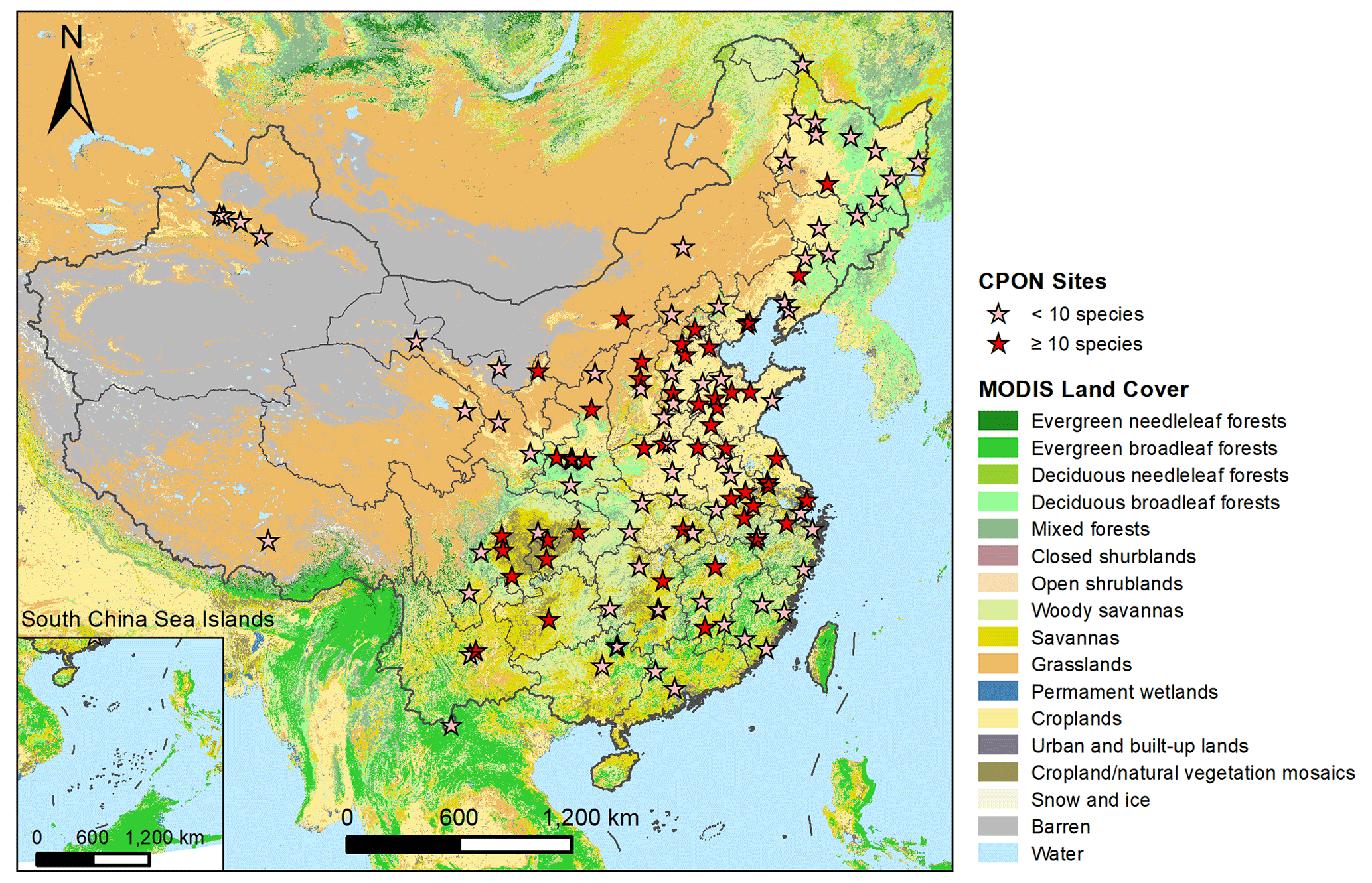
Figure 1 Geographic distribution of CPON sites (n=122) included in the phenology dataset across China. Sites with fewer than 10 recorded species are marked with pink asterisks, while sites with more than 10 recorded species are marked with red asterisks. Note that the markings on the map of several adjacent sites may overlap each other. The background map shows the IGBP land cover type from the MODIS Land Cover product (Friedl and Sulla-Menashe, 2022).

In contrast to manual in situ observations, satellite remote sensing facilitates expansive monitoring and mapping of land surface phenology (LSP) at a landscape scale, yielding more comprehensive phenological data (Studer et al., 2007). Over the past four decades, remote sensing technologies have witnessed substantial enhancements, leading to significant strides in both spatial and temporal resolution (Misra et al., 2020; Dronova and Taddeo, 2022). Currently, a variety of LSP products, based on vegetation indices such as normalized difference vegetation index (NDVI) and enhanced vegetation index (EVI) from diverse remote sensing sources, provide LSP data on regional and global scales with resolutions from 10 km down to 30 m (e.g., Li et al., 2019; W. Wu et al., 2021). The reliability of these LSP datasets is highly dependent on validation against ground phenology (GP) data derived from in situ SP observations (Tian et al., 2021; Zhang et al., 2017), necessitating a seamless transition from individual (i.e., SP) to landscape (i.e., GP) level. Methods such as weighted averages and quantiles have proven their efficacy in this aggregation process from individual to community or landscape levels (Donnelly et al., 2022; Fitchett et al., 2015). For instance, the weighted average method has been validated at the site scale through combined field and remote sensing studies to aggregate GP data from in situ SP observations, considering species abundance as weights (Liang et al., 2011). Recent studies have suggested that quantile methods (e.g., 30th percentile) hold greater promise than the commonly used average methods at larger scales, as demonstrated in Europe and the United States (Ye et al., 2022). Nevertheless, such methods have not yet been applied to aggregate large-scale GP from SP data in China. This gap potentially limits the ground-truthing for LSP products and hampers a comprehensive understanding of the spatial and temporal patterns of phenological shifts over the country.

In this study, we aimed to develop long-term, high-resolution SP and GP maps of China, spanning the period 1951–2020 with a 0.1° resolution. This effort will produce spatially continuous, gridded phenology products that are notably missing in the current Chinese context, yet are vital for diverse scientific and ecological applications. Drawing from the extensive database of the CPON, we analyzed 24 552 in situ phenology observations of 24 representative woody plants from 122 sites over six decades. This analysis included three critical phenophases for each species: the first leaf date (FLD), first flower date (FFD), and 100 % leaf coloring date (LCD). In our methodology, we employed five species-level phenology models with gridded meteorological data to simulate SP maps. To refine these maps for each plant species, we applied species distribution maps as spatial filters. We further synthesized these SP maps into GP maps, utilizing weighted average and quantile methods that incorporated the distribution probabilities of the species as weights. The SP maps underwent a rigorous cross-validation process to ensure accuracy, while the reliability of the GP maps was verified through comparative analysis with existing LSP products. The contribution of this study is the introduction of a novel grid phenology dataset for China. This dataset enhances the spectrum of available phenology data within the country and serves as an independent source for validating LSP products. Moreover, it is expected to significantly advance research on plant phenology and global change by providing a more detailed portrayal of the spatiotemporal trends in plant phenology patterns.

2 Methods

2.1 Data acquisition and processing

2.1.1 Phenology observations

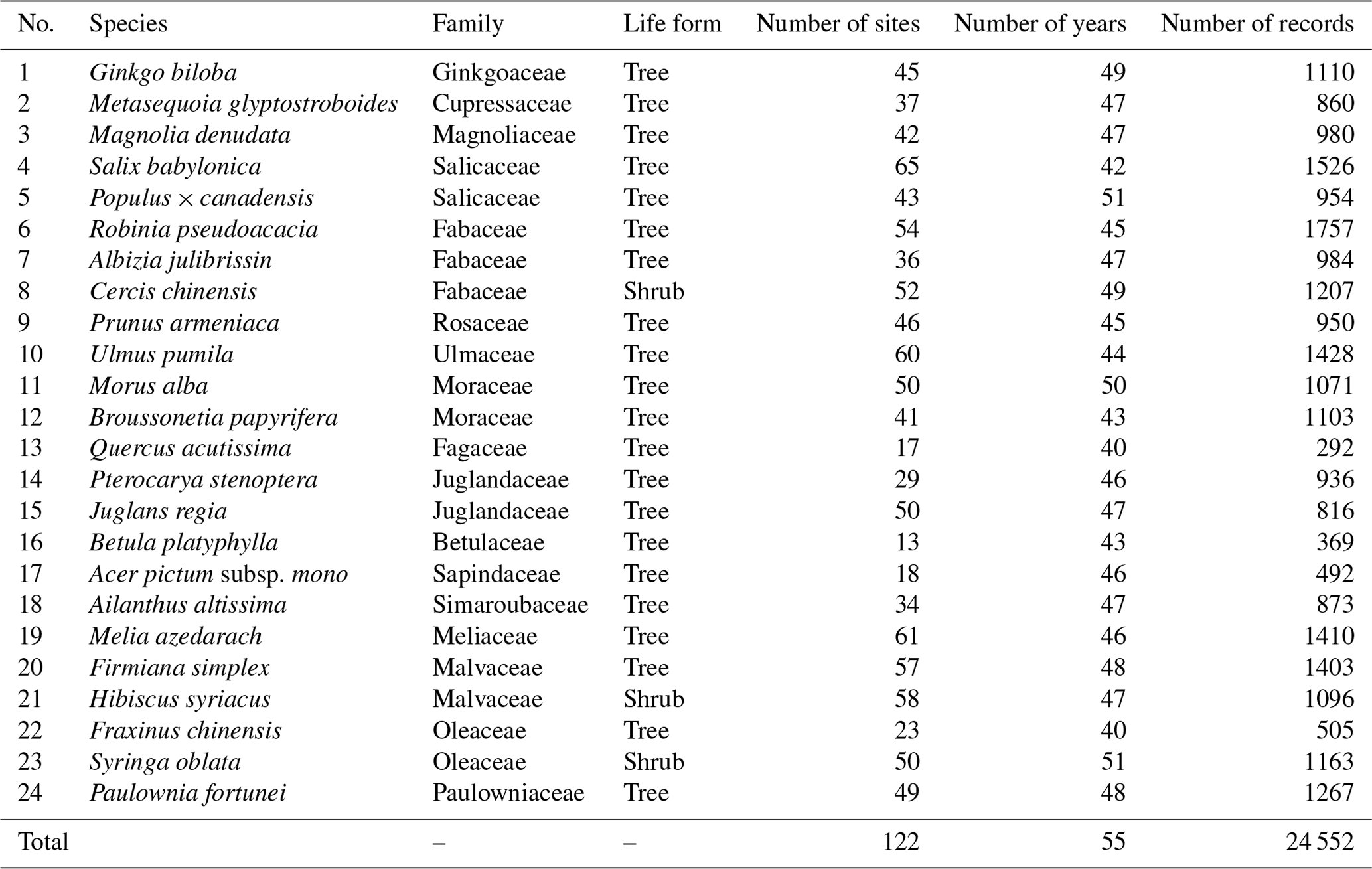
The in situ phenology observations from 1963 to 2018 were obtained from the CPON. We selected 24 representative woody plant species across 17 families (Table 1). These species are not only prevalent in China's forest ecosystems (Fang et al., 2011), but also extensively recorded in the CPON database. The longitudinal span of these observations encompasses 55 years across 122 sites, with a total of 24 552 individual records, covering a diverse spectrum of land cover, ecological, and climatic conditions across China (Fig. 1). Each species in the study has a substantial representation in the dataset, with at least 40 years of phenological data from a minimum of 13 distinct sites. We focused on three phenophases for each species: spring FLD, spring FFD, and autumn LCD. To ensure the integrity of the dataset, we applied three-sigma limits, a statistical filter that retains data within 3 standard deviations from the species mean phenological dates (Pukelsheim, 1994). Outliers that fell beyond these thresholds were excluded, as they constitute less than 1 % of the data points on a standard normal distribution, ensuring a robust and reliable dataset for analysis.

Table 1 List of 24 species of woody plants from 17 families in China. Number of records represents the total number of three phenophases (FLD, FFD and LCD) of all sites and all years for each species.

2.1.2 Climate data

The daily mean temperature (T) data spanning from 1950 to 2020 were sourced from two distinct repositories. (1) Site-specific temperature (Site T) was retrieved from the China Meteorological Data Service Center (CMDSC, https://data.cma.cn/, last access: 1 January 2021). This dataset was primarily utilized for parameterizing the phenology models. (2) Gridded temperature (Grid T) was derived from the ERA5-Land climate reanalysis datasets (Muñoz Sabater, 2019), available through the Copernicus Climate Change Service (C3S, https://cds.climate.copernicus.eu/, last access: 1 August 2022). Grid T was employed for phenology simulation and upscaling processes, with a fine spatial resolution of 0.1°, approximately equating to 10 km. To obtain daily grid T values, we computed the average from hourly temperature data recorded at four distinct times of the day (04:00, 10:00, 16:00, 22:00).

The current bioclimatic variables (BIOCLIM+) were obtained from Climatologies at High Resolution for the Earth Land Surface Areas (CHELSA, https://chelsa-climate.org/, last access: 9 August 2022) to determine the species distribution (Brun et al., 2022a, b). These variables encapsulate the average ecological and climatic conditions for the period 1981–2010, boasting a high resolution of 0.0083°. From the available bioclimatic data, we extracted both the traditional set of 19 bioclimatic layers (Bio1–Bio19) and an additional set of 50 layers. To mitigate the effects of autocorrelation among these bioclimatic variables, we computed the correlation coefficient between each pair of layer. Variables exhibiting a correlation coefficient over 0.8 relative to preceding layers were omitted to prevent redundancy. Consequently, a subset of 12 bioclimatic layers was selected for inclusion as the environmental variables within the species distribution models (detailed in Table S1 in the Supplement). These selected layers were then resampled to a 0.1° resolution to ensure consistency with the resolution of the grid T data.

2.1.3 Forest and species distribution data

The forest distribution map of China was sourced from the dataset of “Annual Dynamics of Global Land Cover and its Long-term Changes from 1982 to 2015” dataset (Liu et al., 2020). To discern forested regions, we reclassified the annual land cover (LC) layers into “forest” and “non-forest” categories. We then determined the duration of forest cover by summing the annual layers, and pixels representing at least 1 year of forest cover were identified as forest distribution areas. For forest type categorization, we employed the widely recognized International Geosphere-Biosphere Program (IGBP) classification system from the MODIS Land Cover Type (MCD12C1) Version 6.1 data product (Friedl and Sulla-Menashe, 2022). In our classification scheme, we combined evergreen needleleaf forest (class 1) and evergreen broadleaf forest (class 2) to delineate evergreen forest category. Similarly, deciduous needleleaf (class 3) and deciduous broadleaf forest (class 4) were amalgamated into deciduous forest category. The mixed forest (class 5) category was retained as is. To achieve a consistent spatial resolution across our datasets, both the forest distribution map and forest type map were resampled from their original 0.05° resolution to a 0.1° resolution using the majority method, so as to match the resolution of the grid T data.

The county-level species distribution maps were sourced from the comprehensive Database of China's Woody Plants (Fang et al., 2011). This authoritative database consolidates distribution data from an exhaustive suite of national, provincial, and regional floristic surveys and inventory reports published in China up to 2009 (Cai et al., 2021). Additionally, we obtained 4371 occurrence records for 24 selected woody plant species from the Global Biodiversity Information Facility (GBIF, 2022; https://www.gbif.org/, last access: 7 September 2022), which were subsequently utilized as the occurrence data inputs for species distribution modeling (detailed in Table S2). To ensure the reliability of our data, we included only those occurrence records that had location coordinates with an uncertainty of less than 2000 m. Moreover, the dataset was meticulously cleansed to eliminate any duplicate records, thereby enhancing the robustness of the species distribution models employed in our analysis.

2.2 Generating species phenology maps using a model-based upscaling method

The generation of SP maps involves two major processes: (1) generating species potential phenology maps, and (2) generating species distribution maps. The definitive SP maps emerged from the spatial intersection of these two distinct map types, effectively overlaying the potential phenology with the actual distribution to pinpoint precise phenological patterns. The workflow for the processes is shown in Fig. 2.

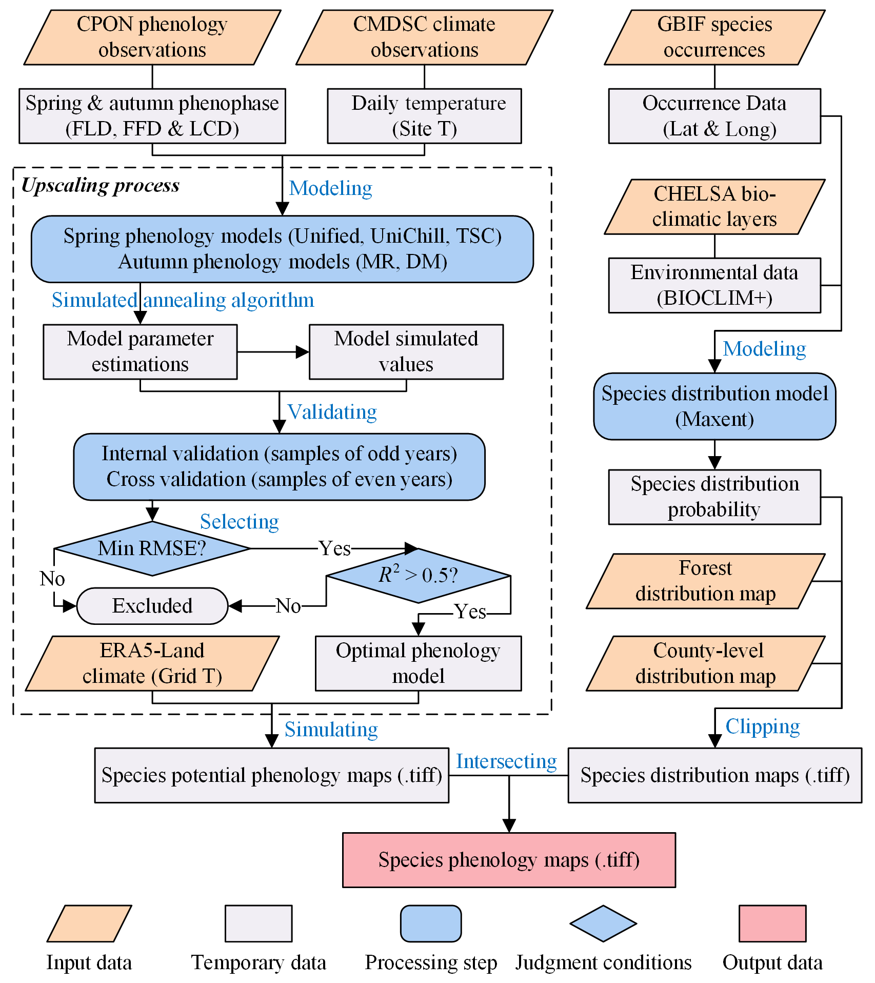
Figure 2 The workflow of generating SP maps using a model-based upscaling method, which involves two major processes: (1) generating species potential phenology maps, and (2) generating species distribution maps. The words in blue represent the key processes of data generation. “.tiff” indicates the GeoTIFF format of the grid phenology or distribution maps.

2.2.1 Species potential phenology maps

In the first process, we employed a model-based upscaling method to transform in situ phenology observations into gridded phenology maps. Phenology models were constructed utilizing the phenophases (i.e., FLD, FFD, LCD) recorded by the CPON, in conjunction with the site T from the CMDSC climate observations. For each species under study, we developed a suite of phenology models for the respective seasonal phases. Three models were designated for spring phenology: the UniChill, Unified (Chuine, 2000) and temporal–spatial coupling (TSC) models (Ge et al., 2014). And two models were designated for autumn phenology: the multiple regression (MR) (Estrella and Menzel, 2006) and temperature–photoperiod (TP) models (Delpierre et al., 2009). The details of the modeling formulae and their respective parameters are elaborated upon in Sect. S1 in the Supplement. The modeling strategy involved a cross-validation approach, where data from odd years were used for model training, while data from even years were set aside for model validation purposes. The estimation of all model parameters was executed via the simulated annealing algorithm (Chuine et al., 1998), ensuring a robust optimization process for the phenology models.

For model validation, the root mean square error (RMSE) and goodness of fit (R²) of the models were calculated between the model-predicted values and the original observed values. We conducted an internal validation using the data from odd years to evaluate the fitting efficacy of the models. On the other hand, we conducted a cross-validation on data from even years to evaluate the capability of the models to simulate and extrapolate phenology data beyond the sample used for model development. The optimal phenology model for each species was determined as the one with the smallest RMSE during the cross-validation process and an R² exceeding 0.5 (or 0.3 for LCD) during both validation processes. Species for which no model met these predefined criteria were omitted from the subsequent generation of SP and GP maps.

To simulate SP maps, we input daily grid T data from ERA5-Land climate reanalysis into the previously determined optimal phenology models for each species. The simulation was conducted on a pixel-by-pixel basis, enabling the interpolation and upscaling of phenology observations from discrete sites to comprehensive gridded phenology maps (Chuine et al., 2000). It is important to note, however, that the availability of grid T data allows for the simulation of species phenology, even in areas lacking observed species distribution. Therefore, we refer to the resultant maps as species potential phenology maps. This distinction emphasizes that while the simulated values represent potential phenological events based on climatic variables, they should not be misconstrued as actual observed values in regions where the species does not exist.

2.2.2 Species distribution maps

In the second process, species distribution maps were generated by integrating species distribution models with county-level species distribution data. For each species, we constructed models using the maximum entropy species distribution modeling (Maxent; Phillips et al., 2006) version 3.4.4. Maxent is a widely utilized tool in species distribution modeling due to its efficacy in estimating the distributional range of a species by finding the distribution pattern with maximum entropy (i.e., closest to the uniform). Maxent models the likelihood of species presence across geographical grids, assigning a predicted probability of occurrence to each grid cell. To configure the Maxent model, we utilized occurrence data from the GBIF database, paired with environmental data inputs from the 12 bioclimatic layers provided by BIOCLIM+. In the model parameter settings, both linear and quadratic feature types were used to capture the relationship between species presence and environmental variables. Additionally, to validate the model and assess its predictive performance, we employed a 5-fold cross-validation method.

To evaluate the accuracy of the Maxent species distribution models, we applied receiver operating characteristic (ROC) curve analysis. The integral of the ROC curve, referred to as the area under the curve (AUC), serves as a quantitative measure of the prediction accuracy of the model (Fielding and Bell, 1997). An AUC value approaching 1.0 is indicative of a model with high predictive accuracy. In our study, the Maxent models demonstrated robust predictive power, with an average test AUC of 0.845 and a standard deviation of 0.043 across the different species (Table S2).

2.3 Generating ground phenology maps using weighted average and weighted quantile methods

In our study, we aggregated individual-level SP maps into landscape-level GP maps using four aggregation methods: (1) weighted average (mean); (2) weighted median (pct50); (3) weighted 20th percentile (pct20) for spring phenology or weighted 80th percentile (pct80) for autumn phenology; (4) weighted 10th percentile (pct10) for spring phenology or weighted 90th percentile (pct90) for autumn phenology. Previous studies typically utilized species abundance as weights for aggregation at a local scale, but obtaining such data at the regional scale proves challenging. Therefore, we replaced species abundance with species distribution probability as aggregation weight for each species. This assumption stems from the positive correlation between species distribution and abundance (Brown, 1984), indicating that species tend to exhibit higher abundance in the core of their geographic range (Sagarin and Gaines, 2002). The aggregation techniques applied in this study (e.g., pct50, pct20\80 and pct10\90) are analogous to the methods used for extracting LSP from remote sensing data (e.g., midpoint, dynamic threshold and maximum curvature). The procedures followed in the generation of GP maps are illustrated in Fig. 3.

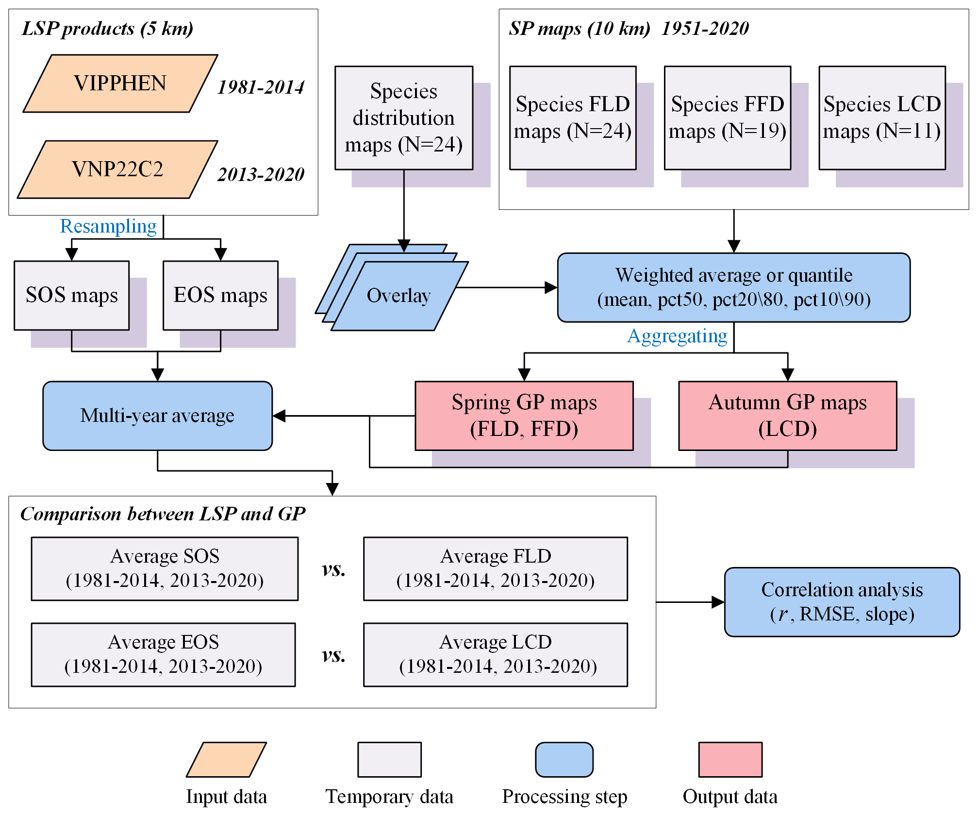
Figure 3 The workflow of generating GP maps from SP maps, and comparing GP maps with two LSP products. The words in blue represent the key processes of data generation.

For n species, the phenological data were first arranged in ascending order. The SP of each species is y_i ($i=\mathrm{1},\mathrm{2},\mathrm{\dots },n)$, and the distribution probability of each species is p_i ($i=\mathrm{1},\mathrm{2},\mathrm{\dots },n)$. Then, the aggregated GP (Y_mean and Y_pct (x %)) was calculated according to the following formulas:

$$\begin{array}{}\text{(1)}& {\displaystyle }{\mathit{\omega }}_i={\displaystyle \frac{p_i}{{\sum }_{i=\mathrm{1}}^n{p}_i}}\text{(2)}& {\displaystyle }{W}_j={\sum }_{i=\mathrm{1}}^j{\mathit{\omega }}_i,j=\mathrm{1},\mathrm{2},\mathrm{\dots },n\text{(3)}& {\displaystyle }{Y}_{\mathrm{mean}}={\sum }_{i=\mathrm{1}}^n{\mathit{\omega }}_i\times y_i\text{(4)}& {\displaystyle }{Y}_{\mathrm{pct}}=\left\{\begin{array}{ll}& y_{\mathrm{1}},\text{if}{W}_{\mathrm{1}}>x\\ (y_j-y_{j-\mathrm{1}})\times & \frac{x-W_{j-\mathrm{1}}}{{\mathit{\omega }}_j},\text{if}{W}_j>x,W_{j-\mathrm{1}}<x\\ & y_n,\text{if}{W}_{n-\mathrm{1}}<x,\end{array}\right.\end{array}$$

where ω_i is a weight to each species, W_j is the cumulative weight from the 1st to the jth species, and x % is the percentile tag which takes values from 10 %, 20 %, 50 %, 80 % and 90 %. These calculations enable the construction of aggregated GP maps by combining species phenology maps with species distribution maps and weighting them by species distribution probability.

To evaluate the data quality and reliability of the aggregated GP maps, we undertook a comparative analysis with two established LSP products derived from remote sensing data: (1) the VIPPHEN_NDVI dataset (1981–2014), which utilized the midpoint method to extract the start of season (SOS) and the end of season (EOS) from the AVHRR data (Didan and Barreto, 2016); (2) the VNP22C2 dataset (2013–2020), which utilized the maximum curvature method to derive SOS and EOS from the MODIS data (Zhang et al., 2020). To align the spatial resolution of these datasets with our GP maps, we resampled both LSP products from 5 km to 0.1° using the average method. Subsequently, we conducted a correlation analysis to assess the consistency between our GP data and the LSP products, specifically comparing the FLD with SOS for the spring, and the LCD with EOS for the autumn. The comparison involved averaging the LSP and GP maps across two distinct periods: 1981–2014 and 2013–2020. The statistical measures calculated for this assessment included the Pearson correlation coefficient (r), RMSE, and linear regression slope between GP and LSP across different forest types (Table S3).

3 Results and discussion

The dataset encompasses two distinct types of phenology maps over China: (1) annual SP maps for 24 woody plants species, constructed using the model-based upscaling method; (2) annual GP maps for forest vegetation, generated by four aggregation methods, accompanied by quality assurance (QA) maps. These maps detail the phenological events of FLD, FFD in spring, and LCD in autumn, spanning from 1951 to 2020, with a spatial resolution of 0.1° and a temporal resolution of 1 d. Each phenology map is stored as a 16 bit signed integer within GeoTIFF file format, comprising a two-dimensional raster (641 row × 361 column). The phenology data are expressed in Julian day of the year (DOY), indicating the elapsed number of days from 1 January to the occurrence of phenological event. The dataset valid DOY values range from 1 to 366, while null values are denoted by −1.

3.1 Simulation and validation of species phenology maps

The SP maps of FLD (24 species), FFD (19 species), and LCD (12 species) were generated by applying the optimal phenology models. Here, we present the results of the SP maps for four emblematic woody species (Fig. 4), including ginkgo (Ginkgo biloba), willow (Salix babylonica), elm (Ulmus pumila), and lilac (Syringa oblata). These maps have been refined using species distribution maps to ensure that the simulated phenologies were relevant only to areas where the species are known to exist. The presented maps illustrate a clear spatial pattern in the timing of phenophases correlated with latitude. Specifically, the onset of spring event such as FLD and FFD for these species is markedly delayed with increasing latitude. Conversely, the autumn LCD occurs earlier as the latitude increases. While these spatial patterns are consistent across species, there are notable temporal differences at the same latitudes, For example, at lower latitudes, the elm exhibits an earlier FFD in spring and a later LCD in autumn compared to the other species. Phenophases for some species were not included in the simulation, because of the suboptimal explanatory power of their phenology models, e.g., R²<0.5 for spring FFD, and R²<0.3 for autumn LCD.

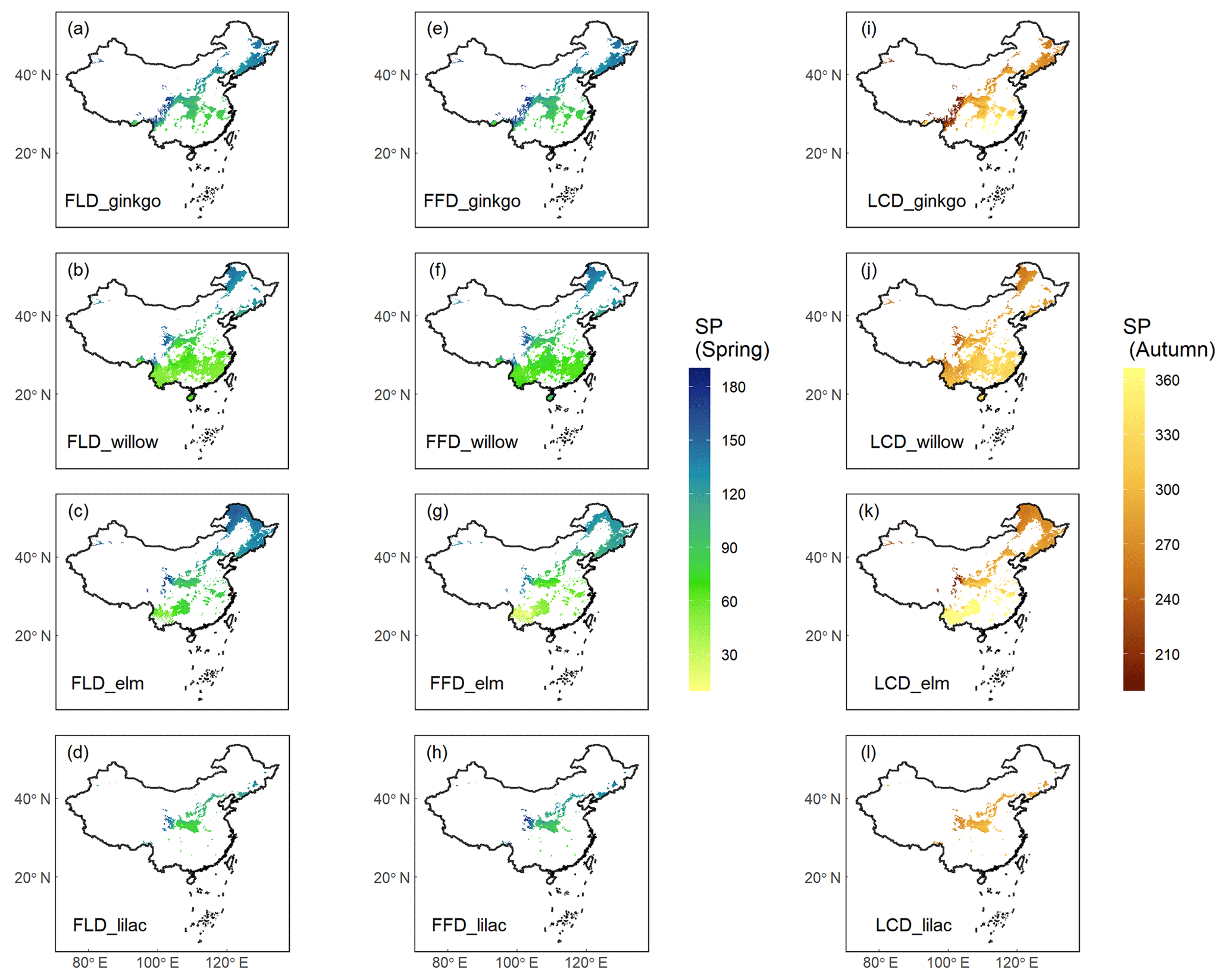
Figure 4 Species phenology (SP) maps of four typical woody species averaged from 1951 to 2020. Columns 1–2 ((a–h)) show the spring phenophases (FLD and FFD), and column 3 ((i–l))shows the autumn phenophase (LCD). Each row represents a species from ginkgo (Ginkgo biloba), willow (Salix babylonica), elm (Ulmus pumila), and lilac (Syringa oblata). The unit of phenology data is the Julian day of year (DOY) from 1 January.

The effectiveness of the simulated SP maps was evaluated by cross-validation on the optimal phenology models (Table 2). The results showed that spring phenology yielded significantly more accurate simulations than autumn phenology (Fig. 5). Quantitatively, the RMSE values for the optimal model of FLD (6.38 d) and FFD (7.46 d) in spring were significantly smaller than that of LCD (10.80 d) in autumn. Correspondingly, the R² for spring FLD (0.799) and FFD (0.676) was significantly higher compared to autumn LCD (0.372). When comparing the simulation effects of FLD and FFD in spring, no significant difference was observed. Among the optimal spring phenology models, the FFD simulations derived from the UniChill and TSC models demonstrated significantly better performance than those from the Unified model. Conversely, for autumn phenology, the simulations effects LCD were comparable between the MR and TP models.

Table 2 The optimal phenology models and cross-validation results of 24 species. RMSE represents the root mean square error between the model simulated values and original values. R² represents goodness of fit of the optimal phenology model.

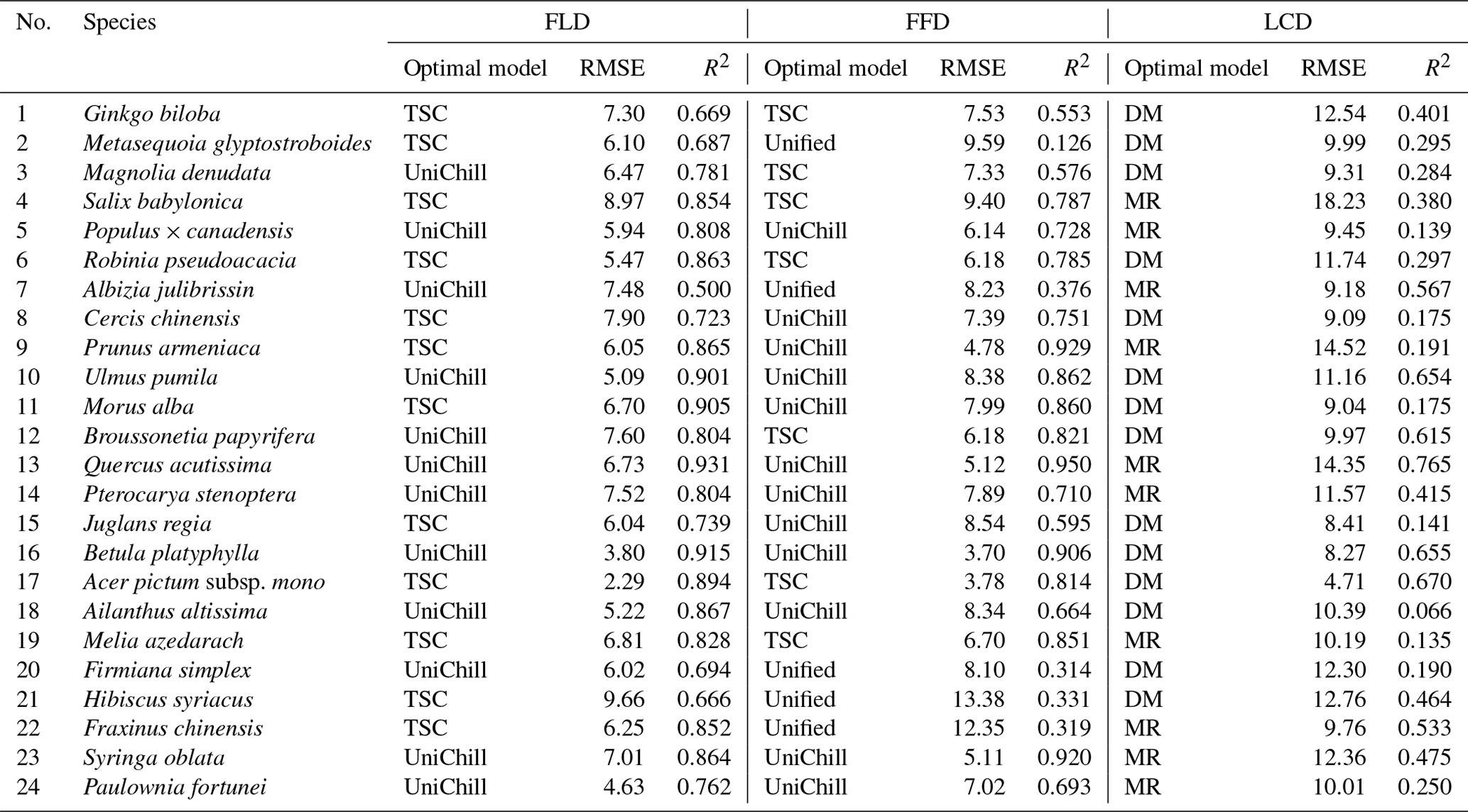
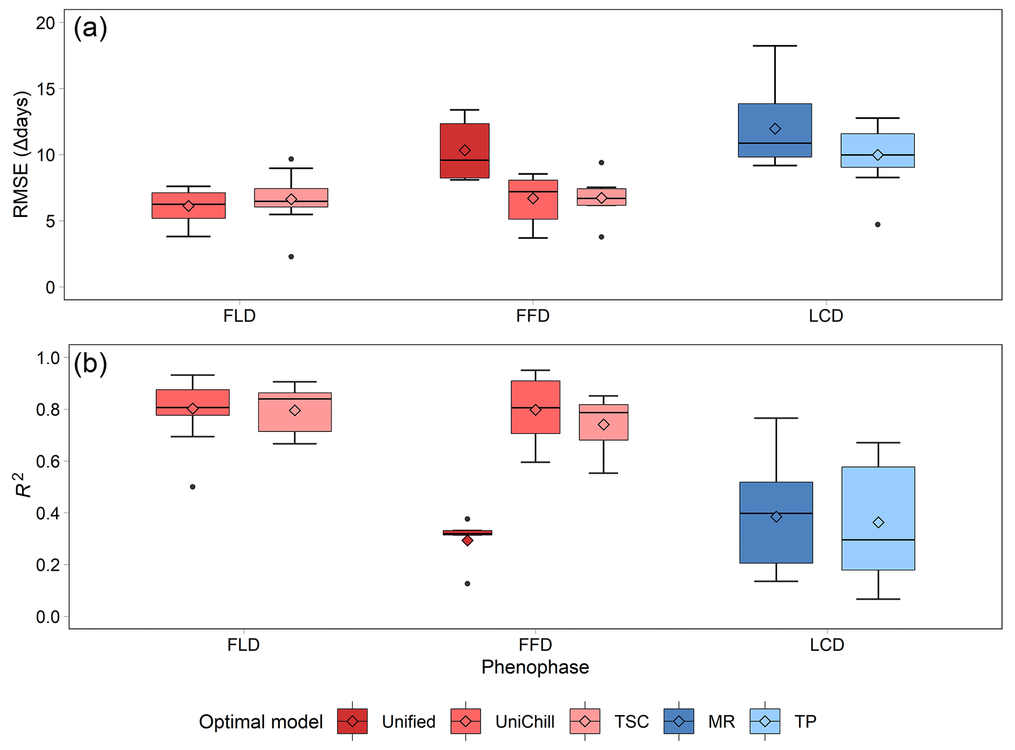
Figure 5 The RMSE (a) and R² (b) of cross-validation on the optimal phenology models for 24 woody species. Each model is represented by a different color, with warm colors for three spring phenology models (Unified, UniChill, TSC), and cool colors for two autumn phenology models (MR, TP). The model with the smallest RMSE was selected as the optimal model for each species. The horizontal line represents the median value, the diamond represents the mean value, and the dot represents the outlier in the boxplot.

3.2 Aggregation of ground phenology maps

The results of GP maps generated by four distinct aggregation methods (mean, pct50, pct20\80, pct10\90) exhibited similar spatial patterns (Fig. 6). These maps demonstrate a consistent pattern of phenological variation in relation to both latitude and altitude. Specifically, with increasing latitude or altitude, spring GP (FLD and FFD) occurred progressively later, while autumn GP (LCD) occurred earlier. When comparing the various aggregation methods, the GP maps aggregated by the mean and pct50 methods showed a high degree of consistency, with r being 0.992. By contrast, the GP maps aggregated by the pct20\80 and pct10\90 methods exhibited slightly more spatial variability and were less correlated with the former methods, with r being 0.968 and 0.949, respectively. The remarkable consistency between the maps aggregated through mean and pct50 methods suggests that both the weighted mean and weighted quantile approaches are robust and reliable for the aggregation of GP.

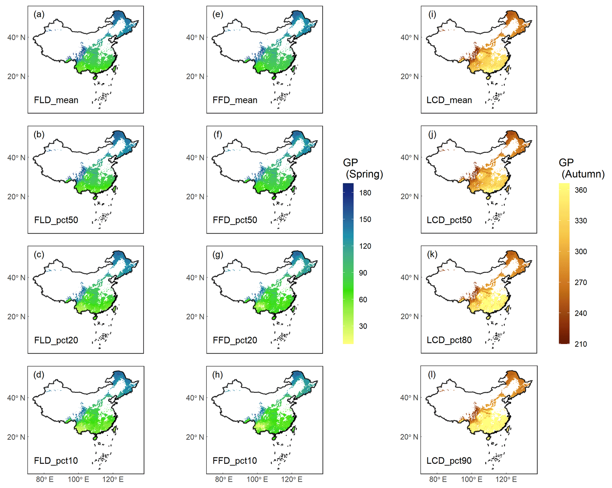
Figure 6 Ground phenology (GP) maps of four aggregation methods averaged from 1951 to 2020. Columns 1–2 ((a–h)) show the spring phenophases (FLD and FFD), and column 3 ((i–l))shows the autumn phenophase (LCD). Each row represents an aggregation method from weighted average (mean), weighted median (pct50), weighted 20 % or 80 % percentile (pct20\80), and weighted 10 % or 90 % percentile (pct10\90). The unit of GP is the Julian day of year (DOY) from 1 January.

We have introduced two types of QA maps to assess the reliability of the aggregated GP maps (Fig. S1). The first QA map represents the total distribution probability of all species considered in the aggregation process, while the second QA map indicates the total number of species that have a distribution probability exceeding 0.1. In these QA maps, higher values correlate with a greater total number or higher cumulative probability of species within the aggregation, which signifies a higher reliability of GP maps for those particular areas. Notably, the most dependable GP aggregation results are distributed around the 30° N latitude within China. In this region, the total number of species contributing to FLD and FFD is about 15, whereas for LCD, the number is around 6. However, it should be noted that the QA maps also identify areas where the GP aggregation may be less dependable. Specifically, in regions where the total number of species is fewer than 5 or the total probability is below 1, the reliability of the aggregated GP results may be compromised.

3.3 Data quality and usability

Our comparative analysis between GP and LSP focused on the FLD and SOS in spring, as well as the LCD and EOS in autumn across two periods (1981–2014 and 2013–2020). The results revealed that GP and two LSP products exhibited congruent spatial patterns in central and northern China, while discrepancies were more pronounced in southern China (Fig. 7), particularly regarding LCD and EOS in autumn (Fig. 7e–h). This is likely due to the prevalence of deciduous forests in central and northern China (Fig. 1). By contrast, southern China is characterized by a higher presence of evergreen and mixed forests. The GP maps in this study were derived from the phenological data of 24 deciduous woody plants species, which are well-represented in deciduous forests but less so in evergreen or mixed forests. Moreover, LSP metrics obtained from remote sensing data are generally more error-prone in evergreen and mixed forests due to the lack of obvious seasonal change and frequent cloud cover in these regions (Y. Liu et al., 2016). Consequently, the correlation between GP and LSP in evergreen or mixed forests was found to be relatively weak (Fig. S2), with the highest r being 0.44 in spring and 0.54 in autumn. and the lowest RMSE being 28.5 d in spring and 38.5 d in autumn (Table S2). In deciduous forests, however, the alignment between GP and LSP was substantially stronger, with the highest r being 0.95 in spring and 0.88 in autumn, and the lowest RMSE being 8.8 d in spring and 15.1 d in autumn, respectively.

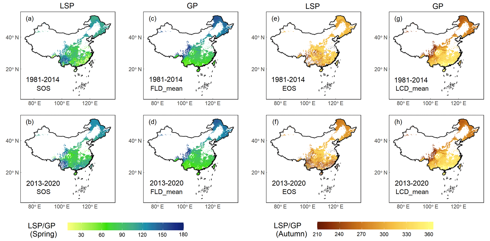
Figure 7 Comparison of GP maps in this study and two LSP products (VIPPHEN and VNP22C2) extracted from remote sensing in previous studies, which was made between FLD and SOS in spring and LCD and EOS in autumn. Row 1 shows the comparison between VIPPHEN product and GP map averaged for 1981–2014, and row 2 shows the comparison between VNP22C2 product and GP map averaged for 2013–2020. (a–b) SOS from two LSP products; (c–d) FLD aggregated by mean method; (e–f) EOS from two LSP products; (g–h) LCD aggregated by mean method. The unit of GP or LSP is the Julian day of year (DOY) from 1 January.

To further assess the data quality, we scrutinized the congruence between GP and LSP specifically within deciduous forests. The analysis indicated that GP and LSP exhibit a robust consistency for both VIPPHEN and VNP22C2 products, characterized by strong correlations, minor differences, and solid linear relationships (Fig. 8). The LSP derived from the VIPPHEN product demonstrated superior consistency with our study's GP compared to the VNP22C2 product's LSP. Furthermore, for both LSP products, the consistency between GP and LSP was significantly better in spring (Fig. 8e, g) than in autumn (Fig. 8f, h). When evaluating the influence of different aggregation methods on the GP and LSP correlation, no significant difference was observed in r among the methods (Fig. 8a, b). The consistency, as measured by r, was comparable across all methods, with values ranging from 0.76 to 0.78 in spring and from 0.49 to 0.53 in autumn for the VIPPHEN product. For the VNP22C2 product, r values ranged from 0.90 to 0.91 in spring and from 0.79 to 0.84 in autumn. Contrastingly, the RMSE between GP and LSP varied notably across the different methods (Fig. 8c, d), which is largely attributable to the disparities in the average GP values generated by each method. The most effective aggregation methods, which yielded the smallest RMSE, were pct10 (20.8 d) in spring and pct90 (32.9 d) in autumn for the VIPPHEN product. For the VNP22C2 product, pct20 (8.8 d) in spring and pct90 (15.1 d) in autumn were identified as the best methods.

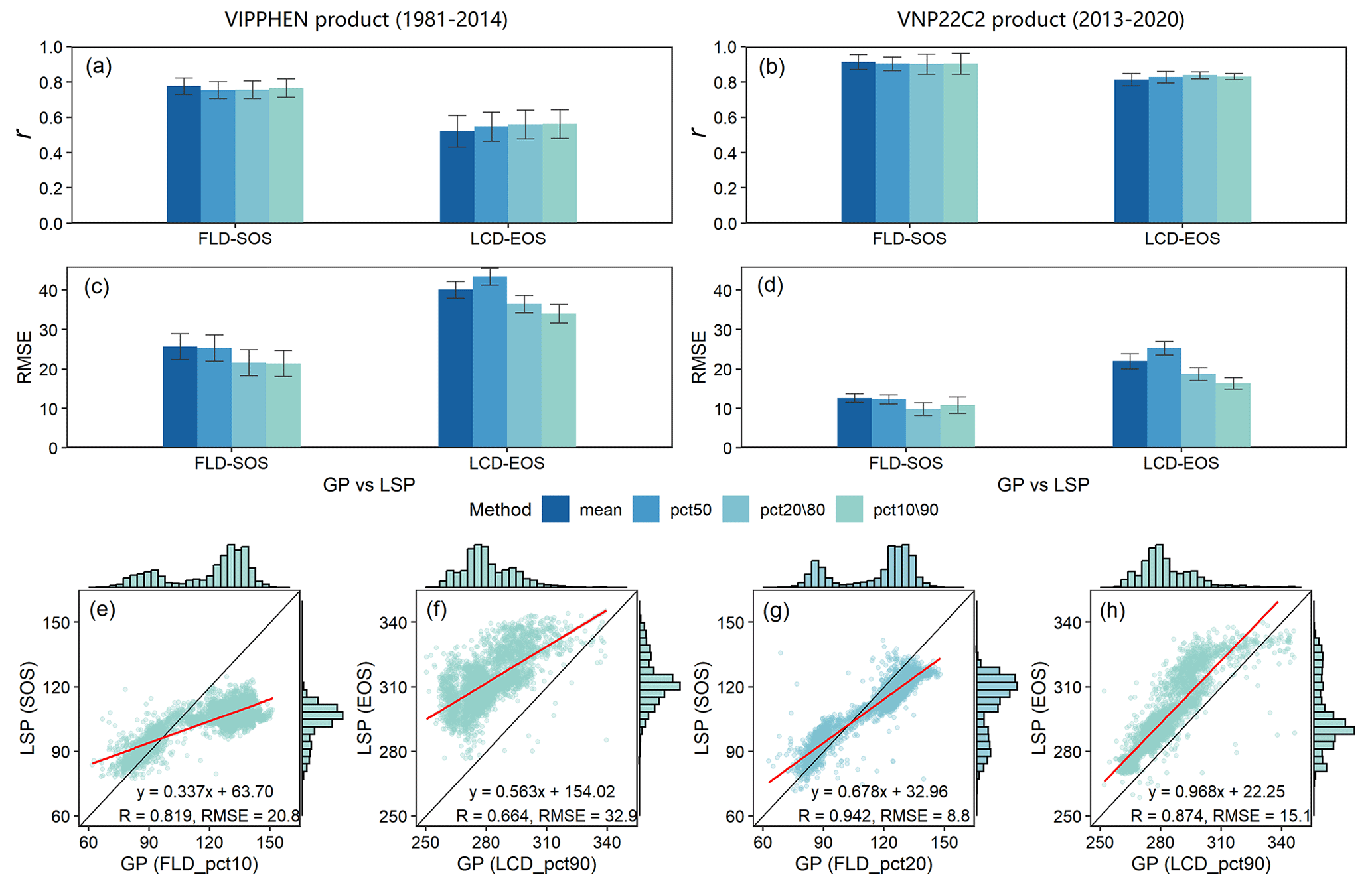
Figure 8 Comparison results of GP maps and two LSP products (VIPPHEN and VNP22C2) in deciduous forests, which was made between FLD and SOS in spring and LCD and EOS in autumn within the time range 1981–2014 and 2013–2020. (a–b) r between LSP and GP under four aggregating methods; (c–d) RMSE between LSP and GP under four aggregating methods; (e–h) linear relationship between LSP and GP under the best aggregating method. Each aggregating method is represented by a different color. The best aggregating method was determined by minimizing the RMSE between GP and LSP. The error bar in the bar plot represents the multi-year standard deviation. The red line in the scatter plot represents the linear regression line between GP and LSP, and all regression results were extremely significant (p<0.001).

The findings of this study highlight that the most accurate reflection of GP in comparison with LSP from remote sensing data occurs with the use of the 10th or 20th percentile for spring phenology and the 90th percentile for autumn phenology. This suggests that the onset of spring as detected by remote sensing aligns more closely with the FLD of the earliest emerging plant species (the first 10 %–20 %) on the ground. Conversely, the signal of vegetative dormancy in autumn from remote sensing is in greater concordance with the LCD of the last senescent plant species (the last 10 %). These insights are significant because they reveal a discernible link between GP and LSP, despite inherent differences in how these two types of phenology are measured. The consistency between early spring and late autumn events in GP and LSP underscores the potential for integrating these two phenological data sources to enhance our understanding of ecosystem dynamics and the effects of climate change on vegetative cycles.

The dataset represents a robust compilation of species and ground phenology simulations for forests of China over the past 70 years, distinguishing itself as an independent phenological data source derived from ground observations through modeling and aggregation. When applying these data, several factors must be considered:

1. For SP maps, the accuracy is contingent upon the RMSE and R² resulting from cross-validation against the optimal phenology model for each species (Table 2). Additionally, the spatial reliability of phenology data is influenced by the density of observational sites per species (Table 1). For instance, while the FLD of Betula platyphylla exhibits high overall accuracy (RMSE = 3.80 and R²=0.915), the accuracy may be compromised locally in areas with fewer observation sites (n=13). Across the 24 species studied, SP maps consistently aligned with the in situ observations, with an average error of 6.4 d for FLD, 7.5 d for FFD, and 10.8 d for LCD. These errors are comparable to or lower than those reported in phenological studies from other regions. For example, simulation error of spring FLD and FFD was 7–9 d in central Europe (Basler, 2016) and 12.3–12.7 d in the United States (Izquierdo-Verdiguier et al., 2018), while the simulation error of autumn LCD was 10.3–13.0 d in France (Delpierre et al., 2009) and 5.9–22.8 d in the United States (Jeong and Medvigy, 2014). Consequently, compared with other studies on the regional scale, the SP maps of China in this study were found to have relatively high accuracy.

2. For GP maps, data reliability can be assessed using QA maps, which reflect the total number or probability of species. Additionally, reliability can be evaluated by comparing GP maps with other LSP products, with a high degree of consistency indicating strong reliability. However, it is crucial to note that GP data primarily represent phenological estimates for deciduous forest components, resulting in higher reliability within deciduous forests and lower within evergreen or mixed forests. In this study, GP maps for forests in China demonstrated strong consistency with existing LSP products, especially within deciduous forests. The correlation coefficients of FLD and LCD were 0.91 and 0.84, respectively. Furthermore, the discrepancies between GP and LSP for FLD and LCD were relatively minor in deciduous forests, at 8.8 and 15.1 d, respectively. Previous studies have reported lower consistency between LSP and single species phenology, with correlations ranging from 0.50 to 0.51 in the United States (Peng et al., 2017) and Germany (Kowalski et al., 2020), and discrepancies spanning 12–14.5 d in the United States (Peng et al., 2017) and Canada (Delbart et al., 2015). On the other hand, research comparing GP aggregates (average or quantile values) of multiple species has yielded better correlation coefficients, ranging from 0.61 to 0.71 in Europe (Rodriguez-Galiano et al., 2015; Tian et al., 2021), and 0.54 to 0.57 for the 30th percentile GP in China (Wu et al., 2016). These studies reported discrepancies between GP and LSP of 10.3–12.4 d in China (Wu et al., 2016), 13.9 d in Europe, and around 12.3 d in the United States (Ye et al., 2022), which are greater than the FLD discrepancies but less than those for LCD found in our study. While the aggregated GP data derived from species-level phenology data in this study are generally reliable, it is important to recognize that limitations still exist in the available species-specific data, particularly when applied to evergreen or mixed forest regions.

3. For phenology maps in different seasons, the phenology data exhibit significantly higher reliability for spring events compared to those in autumn. The underlying reason is that the biological processes underlying autumn phenology are more complex than those of spring (Menzel, 2002). Moreover, the mechanistic drivers of autumn phenology are intricate, which poses an additional challenge (Gill et al., 2015; Wu et al., 2018). For example, temperature has large effects on the autumn phenology than on the spring phenology (Fu et al., 2018). In addition to temperature, other environmental factors such as precipitation (An et al., 2020), photoperiod (Lang et al., 2019), solar radiation (Z. Wu et al., 2021), spring phenology (Q. Liu et al., 2016), and growing-season productivity (Zani et al., 2020) also play significant roles in shaping autumn phenology. Given the multiplicity and complexity of these driving mechanisms, modeling autumn phenology becomes a more daunting task (Melaas et al., 2016). As a result, SP and GP maps for autumn manifest lower model performance and data quality relative to their spring counterparts.

4 Data availability

The annual SP and GP maps over China can be accessed at https://doi.org/10.57760/sciencedb.07995 (Zhu and Dai, 2023). This dataset is licensed under a CC-BY 4.0 license. The spatial reference system of the dataset is EPSG:4326(WGS84).

5 Conclusions

Leveraging historical observations from the CPON, this study introduces a novel, long-term gridded phenology dataset that includes SP maps for 24 woody plants species and GP maps of forests over China, covering the period from 1951 to 2020. The dataset features a spatial resolution of 0.1° and a temporal resolution of 1 d. The SP maps were produced using a model-based upscaling method to extend the phenology data from in situ observations to a regional scale across China. The GP maps were generated by employing weighted average and quantile methods to aggregate phenology data from the species to community and landscape levels. Quality assessments of the dataset indicate an average error for SP maps of 6.9 d in spring and 10.8 d in autumn. The smallest discrepancies between the GP maps and existing LSP products are 8.8 d for spring and 15.1 d for autumn. Compared to the previous studies (Basler, 2016; Delpierre et al., 2009; Izquierdo-Verdiguier et al., 2018; Jeong and Medvigy, 2014; Tian et al., 2021; Wu et al., 2016; Ye et al., 2022), the SP maps from this research exhibit comparable or smaller simulation errors, and the GP maps show strong concordance with other LSP products, underscoring the high accuracy and reliability of the dataset. As the inaugural phenological map set for China, this dataset provides an invaluable tool for discerning the spatial patterns of plant phenology along the geographic gradient (e.g., longitude, latitude, and altitude). It also enables the examination of temporal trends (e.g., interannual, decadal, and secular) in plant phenology throughout China. Moreover, the dataset offers critical support for research on the impacts of global change, aids in terrestrial ecosystem modeling, and contributes to natural resource management strategies.