Multiyear surface wave dataset from the subsurface “DeepLev” eastern Levantine moored station

Processed and analyzed sea surface wave characteristics derived from an up-looking acoustic Doppler current profiler (ADCP) for the period 2016–2022 are presented as a dataset available from the public open-access repository of SEA scieNtific Open data Edition (SEANOE) at https://doi.org/10.17882/96904 (Haim et al., 2022). The collected data include full two-dimensional wave fields, along with computed bulk parameters, such as wave heights, periods, and directions of propagation. The ADCP was mounted on the submerged Deep Levantine (DeepLev) mooring station located 50 km off the Israeli coast to the west of Haifa (bottom depth ∼1470 m). It meets the need for accurate and reliable in situ measurements in the eastern Mediterranean Sea as the area significantly lacks wave data compared to other Mediterranean sub-basins. The developed long-term time series of wave parameters contribute to the monitoring and analysis of the region's wave climate and the quality of wind–wave forecasting models.

1 Introduction

In the past decades, ocean waves have been observed around the Mediterranean sea, in some cases providing prolonged records (Ntoumas et al., 2022; Vargas-Yáñez et al., 2023; Morucci et al., 2016; Pomaro et al., 2018) and, more recently, using high-frequency radars (Lorente et al., 2022). While there are increasing efforts to gather measurements in the sub-basins of the Mediterranean sea (Tintoré et al., 2019), the Levantine basin is still comparably lacking in observations (Toomey et al., 2022). Monitoring ocean waves is crucial for support in making informed decisions related to the development, protection, and management of the marine and coastal environments. Accurate and regular wave measurements are also of great importance in numerous research fields, for example, in studying air–sea and wave–current interactions (Wolf and Prandle, 1999), analyzing climate changes, or investigating the effects of waves dispersion of particles and oil slicks in the water (Fannelop and Waldman, 1972; Sobey and Barker, 1997; Röhrs et al., 2012). Furthermore, the renewable-energy sectors seek to harness ocean waves for power generation, and precise wave monitoring is essential for optimizing the design and operation of wave energy converters (Aderinto and Li, 2018; Lira-Loarca et al., 2021), including in the Levantine basin, where Zodiatis et al. (2014, 2015) estimated the wave energy potential based on a validated wave model.

The acquisition of a long series of surface wave data was made possible with the establishment of the Deep Levantine (DeepLev) station that was deployed for the first time on November 2016 about 50 km offshore Haifa, Israel, at 33°00^′ N and 34°30^′ E. It was the first of its kind: a deep-ocean moored research station in the eastern Levantine basin (ELB) conducting measurements across various fields of marine science. Katz et al. (2020) give a full description of the mooring system and the large number of state-of-the-art measuring instruments it carries. The mooring cable extended from the seabed at a depth of approximately 1470 m up to a subsurface buoy (at a nominal depth of ∼30 m), carrying an up-looking acoustic Doppler current profiler (ADCP). In general, instruments for wave measurements are deployed at shallow and intermediate waters (20–40 m depth), which is a fairly understandable practice considering the added complexity and, hence, the increased costs involved in deep-sea surveys. Nonetheless, long-term observations in deep waters are valuable for continuous monitoring of sea states. Moreover, avoiding the presence of nearshore bathymetry changes or shore reflections allows for a better accuracy evaluation of wave models and satellite measurements.

In this study, a multi-year open-source dataset of wave spectra and derived wave characteristics (i.e., heights, periods, directions) has been developed from DeepLev station measurements for the period 2016–2022. The paper is organized as follows. Section 2 is dedicated to a general description of the measuring instrument and its operation principles and to an evaluation of wave information. Section 3 provides a deeper consideration of the collected data, expanding upon the processing, as well as upon issues that emerged and their implications for the quality. Section 5 finalizes the paper by listing the main results and perspectives of deep-sea measurements and wave monitoring in the ELB.

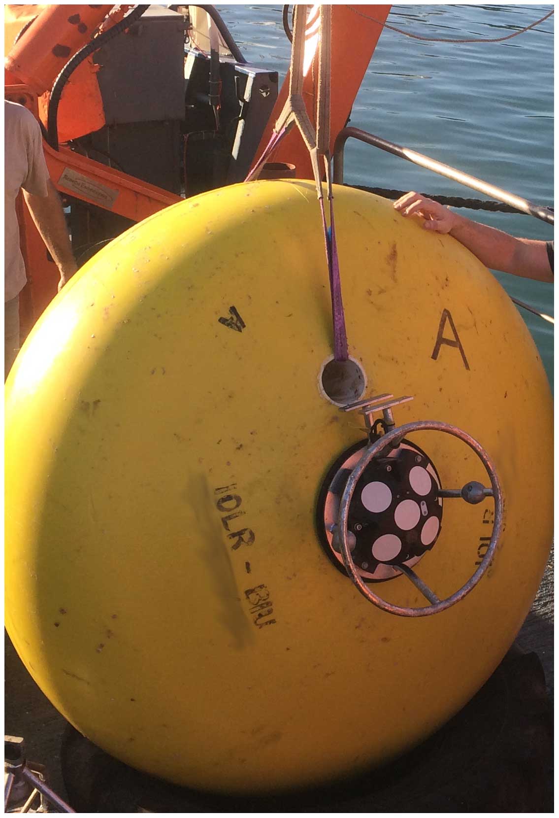
Figure 1 The wave measuring instrument, Nortek's Signature-500, mounted on the top buoy of the DeepLev mooring system.

2 Methodology

2.1 Acoustic Doppler current profiler wave measurements

As was mentioned above, the DeepLev station is a multi-functional research station, monitoring the sea state and marine environment. Throughout the whole campaign, Nortek's Signature-500 ADCP was used to measure surface wave parameters; thus, the derived data are consistent and homogeneous (Fig. 1 shows the subsurface buoy and the ADCP mounted on it). The practice of combining of Nortek's ADCPs and subsurface buoys was found to be successful (Pedersen et al., 2007), though with possible data artifacts due to the buoy's wave induced movement. Compared to Pedersen et al. (2007), in this study, the subsurface buoy was deeper and was therefore expected to be less responsive to the surface waves' motion.

The Signature-500 has three types of sensors: a pressure sensor, four slanted acoustic beams, and a single vertical acoustic beam. This gives it an advantage over other types of ADCPs, allowing for several wave field evaluation approaches to be applied. The first method solely relies on the slanted acoustic beams. The transmitted signals and received Doppler-shifted backscatter (Rowe and Young, 1979; McDaniel and Gorman, 1982) enable an estimation of wave characteristics, including the directional wave spectrum, S^vel(f,θ), from the induced orbital velocities near the surface (Bowden and White, 1966). The main limit of the velocity-based (hereinafter, VEL) method is its sensitivity to installation depth. In deep installations, the horizontal spacing between the beams increases beyond the solution's validity. With the DeepLev's settings, the theoretical upper cut-off at 30 m depth is 3.85 s for directional parameters and 1.15 s for non-directional parameters.

The second method uses the vertically oriented fifth beam for acoustic surface tracking (AST). The measurement of the surface elevation can be directly represented as a frequency spectrum, S^ast(f). Here, even short waves which cannot be detected by the slanted beams' array are visible to the AST. Pedersen et al. (2007) offered a way to expand the surface-tracking information into the directional spectrum, S^suv(f,θ), by combining correlated velocity measurements. This method is known as SUV, suggesting the combination of surface tracking (S) with horizontal velocities (UV). The name references a third method, the established PUV technique (Panicker and Borgman, 1974), which applies similar calculations with pressure observations instead. In this study, the depths of installation make most of the wind–wave frequency ranges undetectable for the pressure sensor; therefore, the pressure fluctuation spectrum, S^puv(f), is not further discussed, though it is included in the dataset as it may be useful to those interested in the low-frequency end of the wind–wave spectrum.

Table 1 Operating duration and configuration for each ADCP deployment.

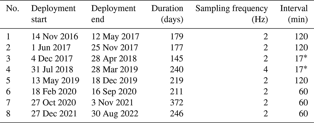
^∗ Continuous-mode measurements which were then processed in 17 min windows.

Prior to each deployment, the device's operation mode was configured to be balanced between the expected duration in the sea and the available battery capacity. Table 1 summarizes the details of the deployments, including the configuration of the experiment, its duration, cycle intervals, and sampling frequency. Most of the time, the ADCP was configured to operate with a sampling frequency of 2 Hz, with the exception of the fourth deployment, where the sampling frequency was 4 Hz. The cycle intervals are regulated by two different modes of Signature-500, namely “burst” mode and “continuous” mode. When set to burst mode, the device worked at intervals and collected only 2048 continuous samples within a cycle (equivalent to about 17 min when using 2 Hz). The intervals between cycles were also predetermined and are listed in Table 1. The third and fourth deployments measured in continuous mode without any pauses. For the purpose of consistency, their measurements were analyzed to provide 17 min averages, as with the rest of the deployments.

2.2 Surface wave averages and directional-property extraction

The first stage of data processing was performed by Nortek's Ocean Contour software, which synthesizes the primary binary files into wave information. The simplest type of analysis provided includes directly identifying individual waves in the surface elevation time series, η(t). Then, wave characteristics are summarized into the maximal measured wave height (H_max) and period (T_max), the mean height (H_mean), the mean zero crossing (T_z), and averages over the heights and periods of the highest $\mathrm{1}/\mathrm{3}$ of the waves (H₃ and T₃) and the highest $\mathrm{1}/\mathrm{10}$ of the waves (H₁₀ and T₁₀).

Additionally, using the fast Fourier transform, the time series signals are converted into a spectral variance density function (S(f)) (Longuet-Higgins et al., 1963) that indicates how much of the surface wave elevation variance is contained at the specific frequencies (f). This spectral representation highlights the peak frequency (f_p), the most energetic frequency inversely related to the peak period (T_p). Other bulk parameters are calculated through the energy spectrum's moments (Tucker, 1993), with the moment of order n defined as

$$\begin{array}{}\text{(1)}& m_n=\underset{\mathrm{0}}{\overset{\mathrm{\infty }}{\int }}{f}^{n}S\left(f\right)\mathrm{d}f,\end{array}$$

where S(f) is the directionally averaged density spectrum. The parameters calculated from the spectral moments are the significant wave height ($H_{m\mathrm{0}}=\mathrm{4}\sqrt{m_{\mathrm{0}}}$); the mean wave period ($T_{m\mathrm{02}}=\sqrt{\frac{m_{\mathrm{0}}}{m_{\mathrm{2}}}}$); and the energy period ($T_{\mathrm{energy}}=m_{-\mathrm{1}}/m_{\mathrm{0}}$), a weighted mean period based on the spectral density, which is useful in estimating wave energy potential. For directional data, the mean wave direction per wave frequency, θ_m(f), is obtained from the first harmonic Fourier coefficients of the power density spectrum function (S(f,θ)) and the corresponding Fourier coefficients (a_n(f), b_n(f)) as follows:

$$\begin{array}{}\text{(2)}& \begin{array}{rl}{\mathit{\theta }}_{\mathrm{m}}\left(f\right)& =\arctan {\displaystyle \frac{b_{\mathrm{1}}\left(f\right)}{a_{\mathrm{1}}\left(f\right)}},\\ a_n\left(f\right)& ={\displaystyle \frac{\mathrm{1}}{S\left(f\right)}}\underset{\mathrm{0}}{\overset{\mathrm{2}\mathit{\pi }}{\int }}S(f,\mathit{\theta })\cos n\mathit{\theta }\mathrm{d}\mathit{\theta },\\ b_n\left(f\right)& ={\displaystyle \frac{\mathrm{1}}{S\left(f\right)}}\underset{\mathrm{0}}{\overset{\mathrm{2}\mathit{\pi }}{\int }}S(f,\mathit{\theta })\sin n\mathit{\theta }\mathrm{d}\mathit{\theta }.\end{array}\end{array}$$

The reported mean wave direction (θ_m) is a weighted average of θ_m(f) in each frequency bin according to its energy. The peak direction (θ_p) is the peak of the spread function constructed employing Fourier coefficients of all available harmonics (n=2) for the peak frequency. Both estimations are expressed here in meteorological conventions; i.e., the specified direction is the direction from which the waves are coming.

The applied methodology provides a complete set of standard wave characteristics and allows us to compare the results with models, satellites, buoys, and visual wave observations on equal terms.

3 Results

The developed dataset presented in this paper includes processed, corrected, and analyzed measurements from eight ADCP deployments for the period 2016–2022. In order to save maximum wave information, we stored all measurements that passed the original Norteks' software quality controlling. However, the data were complemented by quality indexes based on a detailed analysis of observations.

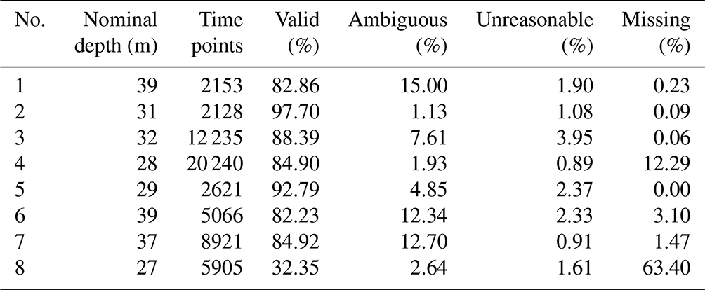
Table 2 Summary of quality indexes for each deployment as described in Sect. 3.2.

3.1 Data integrity and correction

Overall, the observations presented here cover a period equivalent to 4.9 consecutive years, between 14 November 2016 and 30 August 2022. As of the writing of this paper, the DeepLev operation is still ongoing – specifically, it is in its ninth deployment of the wave monitoring ADCP, which began on January 2023 and was recovered in the beginning of 2024 (it will be analyzed and added to the dataset when ready). Table 2 describes the data obtained from each deployment along with assigned quality indexes. Predictably, the majority of observations are of good quality and provide the full set of wave characteristics, including directional information. Soffer et al. (2020) previously compared wave parameters from the DeepLev's first deployment with a simultaneous measurement of a bottom-mounted ADCP which was located 48.5 km away at a depth of 26 m. Both presented a stormy event with reasonable differences given the distance between the locations, providing an initial validation regarding the reliability of Signature-500 measurements from the subsurface buoy. However, in some of the later deployments, we faced several challenges during data processing and analysis. Some of them were resolved, and others are yet to be explained.

The initial challenge we encountered was a considerable variability in the percentages of “ambiguous” data, indicating the inability of the system to determine a local maximum of the wave energy spectra. Naturally, the situation occurs more frequently while the nominal depth of the buoy carrying the ADCP is higher. When installing a moored station with a 1470 m long cable, it was difficult to ensure the precise depth of the subsurface buoy. In practice, the nominal depths varied by 12 m (27–39 m); therefore, some deployments retrieved higher percentages of directional data than others. The analysis showed that, for the specific wave characteristics measured, securing the instrument at 30 m below the sea surface would add another 10 % of valid data to the gathered wave directional information.

Only a small portion of the measurements were found to be unreasonable or completely missing. Occasionally, if there is a problem with returning bursts or if the device has trouble detecting the surface, there will be missing points after processing. Unfortunately, two of the deployments (the fourth and the eighth) had issues resulting in abnormal data loss. During the fourth deployment, it seems like something obstructed the device, as evidenced by notable deviations between the measured distance and pressure. A relatively short time series of the eighth deployment stems from an unexpected malfunction of the memory card.

Another problem was addressed after the initial processing. In both the second and third deployments, the instrument returned without the ordinary temperature readings. Normally, this information is used to evaluate the water's sound velocity (SV), which is necessary to translate the return time of a burst into distance. As a consequence of the fault, the initial processing for these deployments was carried out with Nortek software's default SV value of 1300 m s⁻¹. In practice, the appropriate values for the water properties in that area are around 1550 m s⁻¹. This means that the calculations were performed with SV values that were lower by about 20 %, which led to similar deviations in computed length scales. To correct these values, the missing temperatures were replaced with records by a secondary temperature sensor attached to the pressure sensor. Using these data, the SV was recalculated with the Gibbs SeaWater (GSW) Oceanographic Toolbox (McDougall and Barker, 2011). Then the calculated parameters were adjusted according to the ratio between the new SV and the original ones. A good indication that the correction succeeded could be found in comparing the adjusted distances from the AST measurement to the pressure observations. After the adjustment, the two series differed from each other in the same manner as in the remaining deployments. In this regard, one should consider the fact that the SV used for calculations is constant even if the water column is strongly stratified, as seen during the local summers when, according to the temperature measurements, the thermocline was located above the ADCP. In light of this, the assumption that the measured values fitted the entire water column turns out to be inaccurate. In such a case, the calculations are based on a temperature measured below the thermocline, while the water columns between the device and the surface are likely 8–10 °C warmer. As a result, the uncertainties in SV and wave height estimates could reach 2 %–3 %.

Lastly, observing waves from a submerged subsurface buoy adds complexity since the measurements are carried out from a moving platform. The processing software uses records from the tilt sensors for corrections. However, to get a good reading from the AST sensor, the tilt must be lower than 10°. With the specified DeepLev station mooring settings, there were no instances of angles exceeding this value, with the maximum registered tilt reaching 8°. Additional variability manifests in the horizontal and vertical locations of the subsurface buoy; this is mostly caused by the forces the flow applies to the entire mooring system. In the most extreme case, the buoy descends by 30 m in 6 h, meaning it does experience occasional substantial changes in depth, even within the 17 min windows we used for analysis. These movements can have a slight impact on the quality of the measurement as they depict an average across varying conditions, but, for the most part, this is negligible since a linear detrend is performed prior to wave parameter extraction. Another type of buoy motion is its response to the surface waves. According to the instrument's accelerometer record of the fourth deployment, the buoy experiences horizontal movements which resemble the frequency distribution of surface waves, with a peak around 0.1 Hz. On the other hand, the vertical accelerations' distribution presents as symmetric, centered at 0.125 Hz (8 s wave period), hinting at a resonant response, likely a buoyancy-related natural harmonic. Surface wave components around this frequency regularly induced sway at an order of magnitude of just a few centimeters to tens of centimeters, which could add bias or random error to the directional estimates. Encouragingly, this motion was not as substantial as it appeared to be in Pedersen et al. (2007), probably because the installations were deeper, and the natural frequencies were higher.

3.2 Data review

The developed dataset represents an open source of surface wave characteristics derived from ADCP measurements (https://doi.org/10.17882/96904, Haim et al., 2022). The number of files corresponds to the number of deployments, which simplifies the selection of the time series of interest. The used NetCDF4 format guarantees easy access and eliminates occasional reading errors. Each file contains the time-varying spectra S^ast(f), S^vel(f,θ), and S^suv(f,θ). In addition, each file includes unified arrays of the aforementioned statistical wave parameters, with a preference for values derived from S^suv(f,θ). The frequency range for wave spectra is 0.02–0.45 Hz, with a step of 0.005 Hz. A few isolated events led the ADCP to experience deepening of over 10 m. The maximum recorded depth was 54 m on 20 March 2022, thus lowering the frequency ambiguity limit to 0.195 Hz. A full description of the files, with detailed specifications of each wave parameter, is available in the Appendix.

.

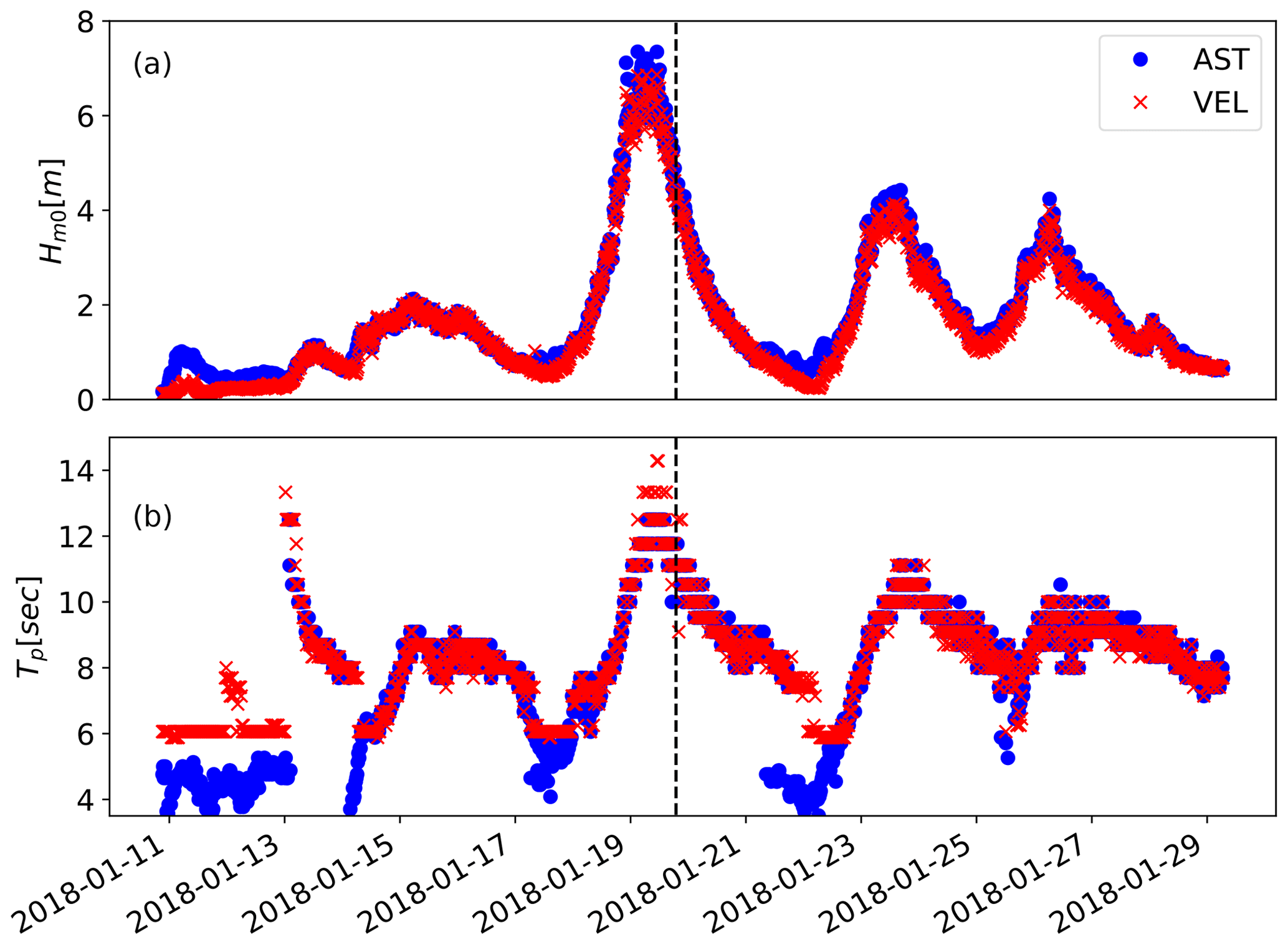
Figure 2 A short time series out of the third deployment derived from velocity orbitals (red) or combined with AST (blue). Shown parameters are (a) significant wave heights and (b) peak period. The vertical dashed line marks the date of the measurements presented in Fig. 4

Figure 2 shows a time series of H_m0 and T_p reconstructed by two methods (VEL and AST) for a short period of the third deployment. This time frame includes the highest observed wave event of the entire campaign, when H_m0 reached 8 m. Apparently, when the surface waves are high and long, there is a good agreement between the two methods. The preference for using the AST approach is eminent in young-wave conditions (Fig. 2b). When it comes to directional spectra, the ability of ADCP is limited in very rough sea states; thus, the example for retrieved spectra is taken after the peak of the event (shown in Fig. 4). Both methods demonstrate a consistency in directional distributions. The incorporation of the AST in the SUV method adjusts the intensities and energy distributions between frequency bins.

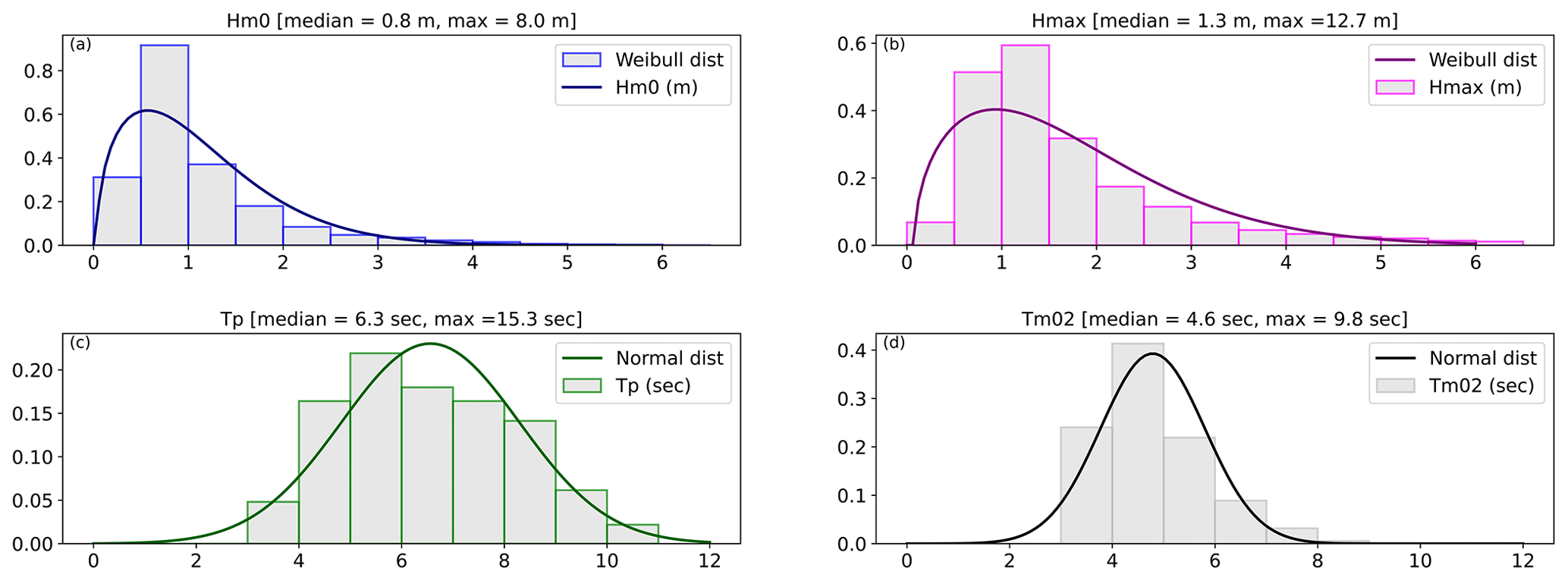
Figure 3 Histograms of combined data from the eight deployments. (a) significant wave heights (H_m0), (b) maximal wave heights (T_max), (c) peak wave periods (T_p), (d) mean wave periods (T_m02). Accompanied by approximated probability fits for comparison.

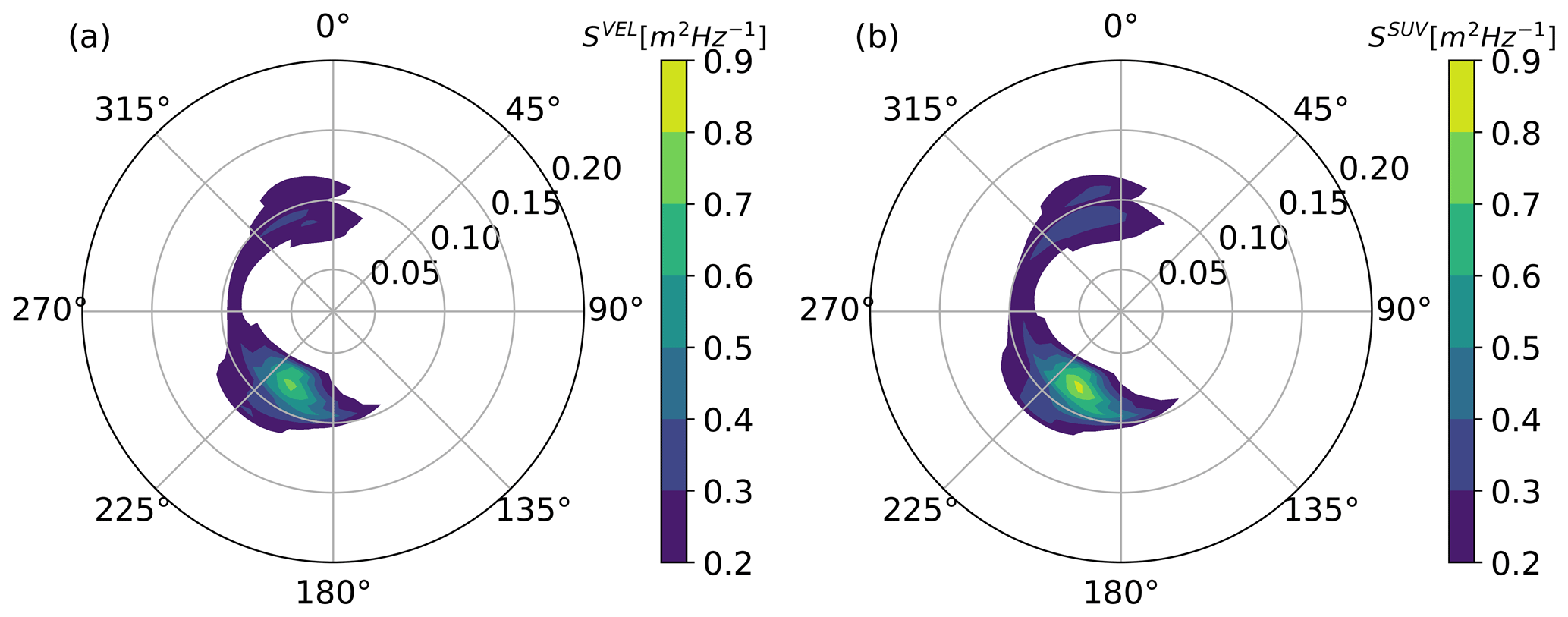
Figure 4 Directional energy density spectra observed on 19 January 2018 at 18:54 UTC, either (a) processed from velocity orbitals (S^vel(θ,f)) or (b) combined with AST (S^suv(θ,f)).

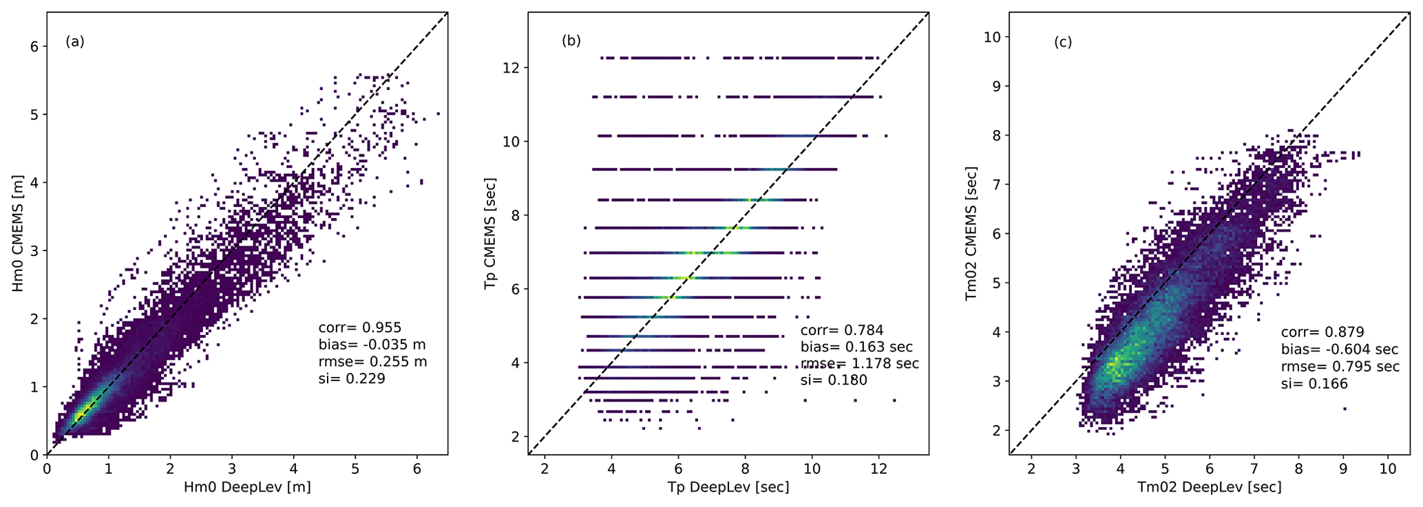
Figure 5 Density scatterplots of the observed (a) H_m0, (b) T_p, and (c) T_m02 values compared to modeled values from CMEMS-WAM between 14 November 2016 and 30 June 2021.

Figure 3 displays the distributions of H_m0, H_max, T_p, and T_m02 among all the data collected. Though there are gaps between deployments, all months were sampled fairly evenly; thus, the results are not expected to be strongly biased. The most probable wave statistics at the DeepLev location have H_m0 between 0.5 and 1 m and a T_p of 5–6 s. Moreover, at least half the time, the H_m0 is over 0.8 m, and finding it measuring up to 2.5 m with H_max of 4 m is common. To give an additional overview of the measured wave distributions, observations between 14 November 2016 and 30 June 2021 are compared with model results from the Copernicus Marine Environment Monitoring Service (CMEMS), which implements the WAM model (Günther et al., 1992; Komen et al., 1996) to simulate waves in the Mediterranean Sea (https://doi.org/10.25423/cmcc/medsea_multiyear_wav_006 _012, Copernicus, 2023). Figure 5 shows the density scatterplots for H_m0, T_p, and T_m02, with the corresponding Pearson correlation coefficient, bias, root mean square error (RMSE), and scatter index (SI). The statistical estimators for H_m0 are comparable to the results of Coppini et al. (2023), who validated CMEMS-WAM using several buoys around the Mediterranean coasts. The correlation coefficient is high, while the other values fall within the range of the buoys. When comparing to the average values of all buoys, the bias and RMSE are more significant. This can be attributed to the bias of forcing winds in eastern Levant, as seen in their comparison to satellite altimetry or the measuring methodology of using an ADCP mounted on a subsurface buoy. The comparison of T_m02 in Fig. 5c shows a general good trend but with a negative bias between modeled and observed values. This bias is not reflected in the T_p scatter, which is concentrated around the best-fit diagonal, meaning the contribution to the bias is mostly caused by the instrument's limit in measuring short waves. Logically, other calculated parameters, like H_m0, could also be affected by the lack of short waves, but as these waves are typically less energetic, the influence is not accentuated. Nonetheless, when working with spectral data, it is recommended that one integrate all parameters of interest only within the instrument's resolved frequency range for optimal comparisons.

4 Data availability

Described data are freely available through the SEANOE (SEA scieNtific Open data Edition) open scientific data repository: https://doi.org/10.17882/96904 (Haim et al., 2022).

5 Summary and conclusion

Wind wave characteristics have been assembled together after multistage data processing, correction, and analysis for an extended period between 2016–2022. The developed dataset, derived from an acoustic Doppler current profiler, is a part of the comprehensive DeepLev monitoring project in the Levantine basin off the Israeli shore. The analyzed data constitute a time series of full two-dimensional wave fields, calculated by two methods utilizing wave orbital velocities and surface tracking, along with conventional statistical parameters: wave heights, periods, and directions of propagation. Preliminary statistical analyses were performed to showcase the distributions, medians, and maximum values of principle wave parameters. Finally, a comparison of observed significant wave heights and mean wave periods to parallel model values shows a gap in estimated periods and an underestimation in the modeling of high waves.

Such a valuable add-on to the exploration of the Levantine Sea is of importance considering the deficiency of observations compared to other sub-basins of the Mediterranean Sea. The collected data can be effectively used for monitoring wave climate changes on seasonal and long-term scales, as well as for the evaluation of extreme wave characteristics or wave energy in the eastern Mediterranean. Beyond the importance of the dataset to this specific region, it is an uncommon extensive time series of deep-water wave spectral measurements, which can generally contribute to marine studies. Besides scientific findings, this experiment has also brought about valuable insights into the long exploitation of the ADCP Nortek Signature-500 in deep waters.

To finalize the paper, we would like to stress the value and importance of a unique 5-year dataset of wave characteristics in the deep waters of the eastern Mediterranean basin for sea state monitoring.

Appendix A

Table A1 The 1D and 2D spectral energy densities included in the NetCDF files. More details on the analysis methods can be found in Sect. 2.

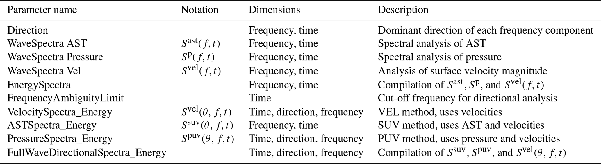
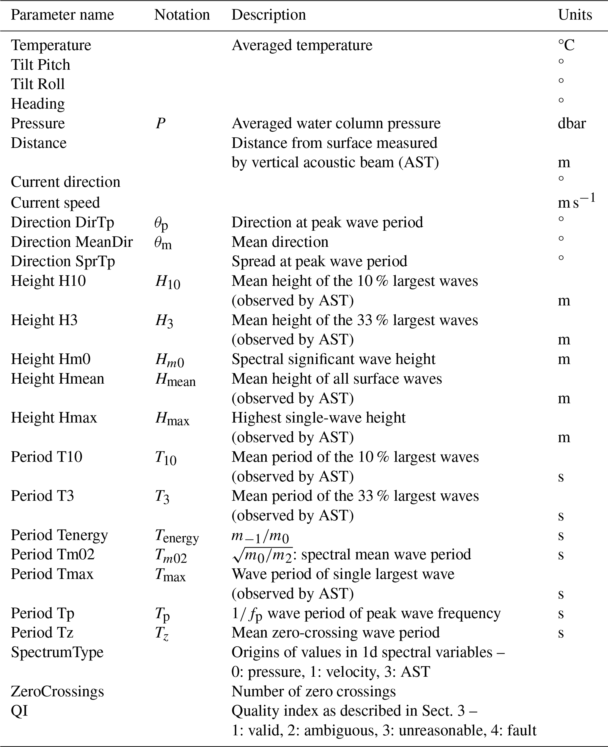
Table A2 Time series of wave parameters and sensor records included in the NetCDF files. Parameter names are as they appear in the files, and notations are as they appear in the text.