the Creative Commons Attribution 4.0 License.
the Creative Commons Attribution 4.0 License.
 | 06 May 2024
SDUST2020MGCR: a global marine gravity change rate model determined from multi-satellite altimeter data
Fengshun Zhu
Huiying Zhang
Lingyong Huang
Heping Sun
Xin Liu
Investigating the global time-varying gravity field mainly depends on GRACE/GRACE-FO gravity data. However, satellite gravity data exhibit low spatial resolution and signal distortion. Satellite altimetry is an important technique for observing the global ocean and provides many consecutive years of data, which enables the study of high-resolution marine gravity variations. This study aims to construct a high-resolution marine gravity change rate (MGCR) model using multi-satellite altimetry data. Initially, multi-satellite altimetry data and ocean temperature–salinity data from 1993 to 2019 are utilized to estimate the altimetry sea level change rate (SLCR) and steric SLCR, respectively. Subsequently, the mass-term SLCR is calculated. Finally, based on the mass-term SLCR, the global MGCR model on 5′ × 5′ grids (SDUST2020MGCR) is constructed by applying the spherical harmonic function method and mass load theory. Comparisons and analyses are conducted between SDUST2020MGCR and GRACE2020MGCR resolved from GRACE/GRACE-FO gravity data. The spatial distribution characteristics of SDUST2020MGCR and GRACE2020MGCR are similar in the sea areas where gravity changes significantly, such as the eastern seas of Japan, the western seas of the Nicobar Islands, and the southern seas of Greenland. The statistical mean values of SDUST2020MGCR and GRACE2020MGCR in global and local oceans are all positive, indicating that MGCR is rising. Nonetheless, differences in spatial distribution and statistical results exist between SDUST2020MGCR and GRACE2020MGCR, primarily attributable to spatial resolution disparities among altimetry data, ocean temperature–salinity data, and GRACE/GRACE-FO data. Compared with GRACE2020MGCR, SDUST2020MGCR has higher spatial resolution and excludes stripe noise and leakage errors. The high-resolution MGCR model constructed using altimetry data can reflect the long-term marine gravity change in more detail, which is helpful in studying seawater mass migration and its associated geophysical processes. The SDUST2020MGCR model data are available at https://doi.org/10.5281/zenodo.10701641 (Zhu et al., 2024).


The Earth's large-scale mass migration can cause spatiotemporal changes in the Earth's gravity field (Li et al., 2021). The ocean accounts for about 71 % of the global area, and the determination of time-varying marine gravity field is an important research topic of the Earth's time-varying gravity field. The high-precision and high-resolution spatiotemporal change information of the marine gravity field is useful for monitoring related geophysical processes such as ice melting, ocean dynamic processes, and crustal deformation.
Investigating the Earth's time-varying gravity field mainly relies on repeated observations of ground gravity and satellite gravity. The large-scale regional gravity field changes can be studied by utilizing the multi-year gravity measurement data on the relative gravity surveying network (Liang et al., 2016). The precise gravity field changes in small areas can be investigated using repeated measurement data from absolute gravimeters at gravity stations (Greco et al., 2012). However, gravimeter observations are costly, and gravimeter marine observations require a lot of human, material, and financial resources. Satellite gravimetry provides the possibility for repeated observations of the Earth's large-scale gravity field. At present, high–low satellite-to-satellite tracking, low–low satellite-to-satellite tracking, and satellite gravity gradient measurement technologies have been developed. Successfully launched gravity satellites include CHAMP, GRACE/GRACE-FO, and GOCE (Flechtner et al., 2021). Among them, the GRACE/GRACE-FO gravity satellite data are the most widely utilized. GRACE/GRACE-FO adopts the gravity measurement technology of the low–low satellite-to-satellite tracking model. GRACE/GRACE-FO can obtain time-varying gravity with an accuracy of about 0.1 mGal (milligal; Flury and Rummel, 2005) and time-varying equivalent water height with an accuracy of approximately 1 cm (Wahr et al., 2004), but its spatial resolution of one-half wavelength is only 400–500 km (Tapley et al., 2004), the resolution is low, and there is large signal distortion and leakage errors.
The satellite altimetry technique can quickly and repeatedly obtain high-precision global ocean information, which is becoming an important means to observe and study the ocean. Products such as the mean sea level model, static marine gravity field model, and sea level change dataset can be extracted or derived by using altimetry sea surface height (SSH). The Technical University of Denmark team focused on model improvement in the Arctic Ocean, utilizing multi-satellite altimetry data to construct a global mean sea level model (Andersen et al., 2021, 2023) and a global marine gravity field model (Andersen and Knudsen, 2020). The Shandong University of Science and Technology (SDUST) team also constructed a global mean sea level model (Yuan et al., 2023) and a marine gravity field model (Zhu et al., 2022) using altimetry data, and the accuracy of the model was improved in the offshore region. The European Copernicus Marine Environment Monitoring Service used altimetry data to produce and release daily and monthly gridded sea level change dataset products (Taburet et al., 2019). The Scripps Institution of Oceanography in the United States also developed a global altimetry marine gravity field model (Sandwell et al., 2021). So far, the altimetry SSH has been at the centimeter-level accuracy, and the calculated global sea level changes have reached millimeter-level accuracy (Nerem et al., 2010). The global altimetry marine gravity field model has had a spatial resolution better than 10 km, and the calculation accuracy has been about 1 mGal (Sandwell et al., 2013). However, few studies have applied altimetry means to time-varying marine gravity. This paper aims to utilize multi-satellite altimetry data to construct a global marine gravity change rate (MGCR) model (SDUST2020MGCR).
Seawater migration causes changes in the Earth's shape and gravity field. In this study, we propose to utilize the sea level change rate (SLCR) to calculate the MGCR. Firstly, multi-satellite altimetry data from 1993 to 2019 are utilized to estimate the long-term altimetry SLCR, and EN4.2.1 ocean temperature and salinity data from 1993 to 2019 are utilized to estimate the long-term steric SLCR. Then, the steric SLCR is subtracted from altimetry SLCR to calculate the mass-term SLCR. Finally, this paper applies the method proposed by Zhu et al. (2023) to estimate long-term MGCR, that is, utilizing the mass-term SLCR to construct a global MGCR model based on mass load theory and the spherical harmonic function method. In Sect. 2, the study area and data sources are introduced. In Sect. 3, the methods of altimetry SLCR estimation, steric SLCR estimation, mass-term SLCR estimation, and MGCR estimation are described in detail. In Sect. 4, the global SLCR and MGCR models are given, and the model comparisons and analyses are performed. In Sect. 5, the conclusion is presented.
2.1 Study area
In this paper, the global ocean covering 0–360° E and 70° S–70° N is selected as the study area, as shown in Fig. 1. There are various mass migration phenomena on Earth, such as ocean currents that move seawater in a certain direction, the subduction of oceanic plates to continental plates that form island arcs (e.g., Nicobar Islands) and trenches, and the melting ice due to global warming that reduces the mass of Greenland and Antarctica. The mass migration causes changes in the Earth's gravity field. Constructing the high-resolution time-varying marine gravity model is helpful for the study of the material migration movement.
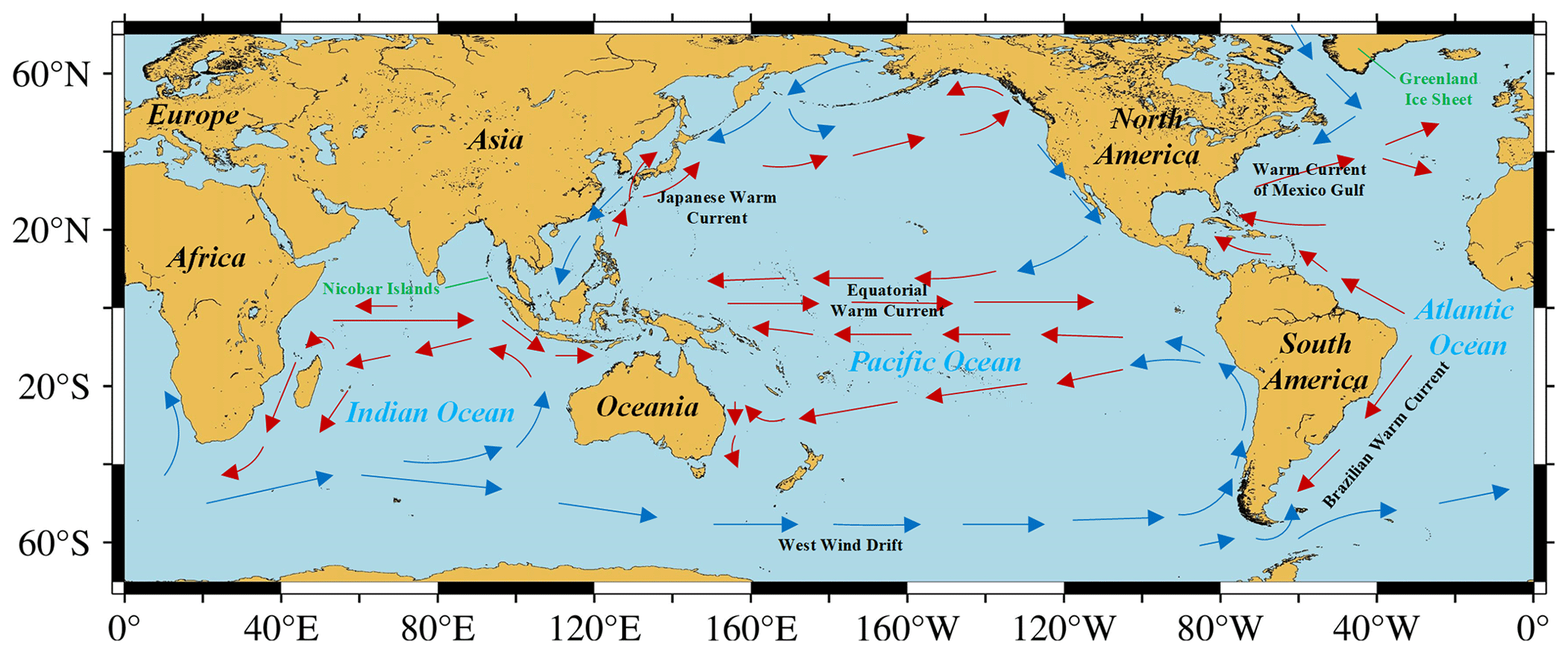
Figure 1The study area covers 0–360° E and 70° S–70° N. The base map was created using Generic Mapping Tools, then we have roughly marked the continents, the oceans, and the local sea areas with obvious gravity changes. Red arrows indicate areas where warm currents pass, whereas the blue arrows indicate areas where cold currents pass; the Nicobar Islands and Greenland ice sheet are also marked in green.
2.2 L2P satellite altimetry data
The satellite altimetry data includes products at different levels: level-0 (L0), level-1 (L1), level-2 (L2), level-2 plus (L2P), and level-3 (L3). The L0 product is raw telemetered data. The L0 product is corrected for instrumental effects to obtain the L1 product. The L1 product is corrected for geophysical effects to obtain the L2 product. The geophysical effect corrections include corrections for dry and wet tropospheric effects, ionospheric effects, ocean state bias, ocean tides, solid tides, polar tides, and atmospheric pressure. The L2 product is also called the Geophysical Data Records (GDR) product. Based on the L2 product, the correction model is updated and replaced, and a new quality control is carried out, such as data validation, data editing, and algorithmic improvement; finally, the L2P product is produced (CNES, 2020). The L3 product is processed river- and lake-water-level time series data.
The L2P product is released by the AVISO (Archiving, Validation and Interpretation of Satellite Oceanographic) data center (https://www.aviso.altimetry.fr/, last access: 6 November 2023) of the French Centre National d'Études Spatiales (CNES). The L2P product includes data such as sea level anomaly, mean sea level, environmental parameters, and geophysical correction models. Therefore, the L2P product can be utilized to calculate the required SSH. This study utilizes SSH data derived from the L2P product to calculate multiple mean sea level models and construct sea level time series data; finally, the least squares model is applied to estimate high-resolution SDUST altimetry SLCR (Yuan et al., 2021).
In this study, the L2P product from January 1993 to December 2019 is selected, including two observation missions of 12 altimetry satellites, as shown in Fig. 2. The ERM (Exact Repeat Mission) data are observed by ERS-1/2, TOPEX/Poseidon (T/P), GEOSAT Follow-On (GFO), Envisat, Jason-1/2/3, HaiYang-2A (HY-2A), SARAL, and Sentinel-3A; the GM (Geodetic Mission) data are observed by ERS-1, Jason-1/2, HY-2A, CryoSat-2, and SARAL.

Figure 2The multi-satellite altimetry data are utilized in this study. The horizontal axis marks the observation time, and the vertical axis marks the name of the altimetry satellite. Blue represents ERM (Exact Repeat Mission) data and orange represents GM (Geodetic Mission) data.
2.3 EN4 ocean temperature and salinity data
The ocean temperature and salinity data are important basic data for studying global climate change and ocean change. These data can be used to study ocean volume changes caused by changes in seawater temperature and salinity and further used to predict global climate disasters. The Argo (Array for Real-Time Geostrophic Oceanography) project aims to use Argo floats to form a global ocean observation network to measure the depth, temperature, salinity, and other parameters of the ocean in real time (Riser et al., 2016). Now, nearly 4000 Argo floats are in working condition, which provide basic data for constructing global ocean temperature and salinity data products.
The various ocean temperature and salinity data products are all affected by irregular float distributions and model gridding, and their accuracy is basically the same (Hosoda et al., 2008; Roemmich and Gilson, 2009). This study utilizes the EN4.2.1 monthly ocean temperature and salinity product from January 1993 to December 2019 released by the UK Met Office (https://argo.ucsd.edu/data/argo-data-products/, last access: 6 November 2023) to study the ocean volume change and calculate the steric SLCR. The grid size of EN4.2.1 data is 1° × 1° (Good et al., 2013).
2.4 AVISO monthly sea level anomaly data
The AVISO data center of CNES also released a monthly sea level anomaly data product on 15′ × 15′ grids. The sea level anomaly is referenced to the mean sea level from 1993 to 2012. This product can discern sea level changes on a scale of 150–200 km, with an accuracy of centimeters in most sea areas worldwide (Ducet et al., 2000). The AVISO monthly sea level anomaly data integrate observation data from Jason-1/2/3, T/P, Envisat, ERS-1/2, GEOSAT, and GFO, and the have been corrected for geophysical influences, such as dry and wet tropospheric influence, ionospheric delay, tides, and the dynamic atmosphere. This study utilizes AVISO monthly sea level anomaly grid data from January 1993 to December 2019 to estimate AVISO altimetry SLCR.
2.5 ICE-6G glacial isostatic adjustment model
The glacial isostatic adjustment (GIA) is the response of the viscoelastic Earth to changes in surface ice and seawater load during the last glacial period. The marine gravity changes resolved from satellite gravity data and satellite altimetry data include not only the impact of contemporary Earth mass migration, but also include the impact of solid Earth mass redistribution driven by GIA. In the research on various Earth science issues, the GIA effect is usually deducted as a linear term. Argus et al. (2014) and Peltier et al. (2015) provided the ICE-6G fully normalized geopotential trend coefficients and , with the degree and order fully expanded to 256. In this study, the degree of the GIA model is truncated to 60, which will be deducted from GRACE and altimetry observations. The spherical harmonic coefficients in the ICE-6G model correspond to the interannual trend, and we need to calculate the GIA coefficients for each month to deduct the GIA effect from the GRACE monthly harmonic coefficients. Based on the ICE-6G fully normalized geopotential annual trend coefficients and , the GIA-corrected geopotential coefficients and for each month from January 1993 to December 2019 can also be calculated:
where N represents the month, and there are 324 months from January 1993 to December 2019. The GIA-corrected geopotential annual trend coefficients and GIA-corrected geopotential coefficients are utilized to correct the altimetry MGCR and GRACE/GRACE-FO monthly gravity data, respectively, which can deduct the marine gravity changes due to the long-term oceanic crust deformation driven by GIA.
2.6 GRACE/GRACE-FO monthly geopotential spherical harmonics data
The main purpose of the GRACE system and the GRACE-FO system is to obtain the long-to-medium wavelength signals of the Earth's gravity field and to detect gravity changes (Han et al., 2004). The orbit parameters of the GRACE satellite and GRACE-FO satellite are basically the same, with an orbit inclination of 89.5° and an orbit altitude of about 500 km (Wouters et al., 2014). The main instruments carried by the satellites are GPS receivers and ranging systems. The GRACE/GRACE-FO time-varying gravity data mainly consist of level-1, level-2, and level-3 data. The level-1 data are raw observations that include distance changes between the dual-satellites, and acceleration changes due to the Earth's gravitational variations. The level-2 data are global time-varying gravity field model expressed as spherical harmonic coefficients, which has been corrected for the effects of ocean tides, solid tides, atmosphere tides, pole tides, and non-tidal variability in the atmosphere and ocean (UTCSR, 2018). The level-3 data are grid format data represented by Mascon products.
The Center for Space Research at the University of Texas (UTCSR) released GRACE/GRACE-FO level-2 RL06 monthly geopotential spherical harmonics data, including CSR_GSM and CSR_GAD data. The CSR_GSM data represent the estimation of Earth's monthly average gravity field, and the degree and order are fully calculated to 60. The CSR_GAD data represent the impact of non-tidal oceanic and atmospheric pressure on the ocean bottom pressure. The International Center for Global Earth Model (ICGEM, http://icgem.gfz-potsdam.de/home, last access: 6 November 2023) provides CSR_GSM data filtered by DDK2 (Kusche, 2007). This is a non-isotropic filtering method, and CSR_GSM_DDK2 contains less stripe noise.
The GRACE/GRACE-FO dataset has 180 months of data between April 2002 and December 2019, and any missing GRACE/GRACE-FO data are not reconstructed in this study. The degree-1 coefficients supplementation and degree-2 and degree-3 coefficients replacement are performed on CSR_GSM_DDK2 data. In addition, to match with the satellite altimetry data, the spherical harmonic coefficients of CSR_GSM_DDK2 and CSR_GAD are linearly summed:
The mean spherical harmonic coefficient of 180 months of gravity data is utilized as the reference gravity field, and the GRACE/GRACE-FO geopotential spherical harmonic coefficient variations, and , are calculated. Then the monthly equivalent seawater height (ESH) change is calculated (Wahr et al., 1998; Godah, 2019):
where λ and θ are the geocentric longitude and colatitude of the calculation point, a=6378136.3 m is the Earth equatorial radius, ρE=5514 kg m−3 is the Earth average density, ρS=1028 kg m−3 is the seawater average density, l and m are the degree and order of the spherical harmonic coefficient, is the fully normalized associated Legendre function, and k is the load Love number.
In this study, the GIA-corrected geopotential coefficient is subtracted from the GRACE/GRACE-FO geopotential spherical harmonic coefficient variations:
Then the monthly gravity change is calculated (Godah, 2019):
where r is the geocentric radius, GM is the Earth's gravitational constant, and other variables are the same as before. This study applies the forward modeling method to correct signal leakage errors on GRACE/GRACE-FO ESH time series data and gravity time series data. Finally, the least squares model is applied to estimate the GRACE/GRACE-FO mass-term SLCR and MGCR, and the grid size is 1° × 1°.
The submarine plate motion, the melting of glaciers and ice sheets, and the changes in ocean dynamics all lead to the spatial distribution changes of seawater mass, which in turn causes changes in Earth's shape and gravity field. In static marine gravity field studies, the geoid height is obtained by subtracting the mean sea surface topography from the instantaneous altimetry SSH, and then the geoid height or geoid gradient is utilized to construct the gravity field model (Gopalapillai and Mourad, 1979; Hwang et al., 2002). In this study of time-varying marine gravity based on satellite altimetry, the mean sea surface topography is also regarded as invariable, and it is proposed to utilize sea level change to study marine gravity change.
The flowchart of this research is shown in Fig. 3. Firstly, following the data grouping, editing, and preprocessing of L2P satellite altimetry data, multiple mean sea level models are calculated to construct altimetry sea level time series data, and then the high-resolution SDUST altimetry SLCR is estimated by applying the least squares model and is compared with the AVISO altimetry SLCR. Then the SDUST mass-term SLCR is calculated by subtracting the EN4 steric SLCR from the SDUST altimetry SLCR, and it is compared with the GRACE/GRACE-FO mass-term SLCR. Finally, based on the SDUST mass-term SLCR, the spherical harmonic analysis, GIA effect deduction, and spherical harmonic synthesis are performed to obtain the SDUST MGCR, and the SDUST MGCR is compared with the GRACE/GRACE-FO MGCR.

3.1 Estimation of altimetry SLCR
3.1.1 Data grouping and editing
The L2P satellite altimetry data from January 1993 to December 2019 are utilized to construct the high-precision and high-resolution altimetry SLCR model. The obliquity between the Moon's orbit and the Earth's Equator is called the lunar declination angle, with a maximum value of 28.5° and a minimum value of 18.5°, and its change cycle is 18.6 years. This study uses a 19-year moving window and a 1-year moving step to divide the L2P products into nine groups (1993–2011, 1994–2012, 1995–2013, 1996–2014, 1997–2015, 1998–2016, 1999–2017, 2000–2018, 2001–2019) (Yuan et al., 2020a), which can attenuate the ocean effect of a typical tide with 18.6 years. In addition, in order to improve the modeling accuracy, the low-quality SSH data are excluded according to the thresholds for altimeter, radiometer, and geophysical parameters defined in the L2P product handbook (CNES, 2020).
3.1.2 Data preprocessing
Each group of SSH data needs to perform the ocean variability correction to attenuate SSH anomalous variation, SSH seasonal variation, and radial orbit error. For the ERM data, the collinear adjustment method is applied to perform ocean variability correction (Rapp et al., 1994). The steps of this method are as follows: firstly, the track with the most observation points among all collinear tracks is selected as the reference track; then, the SSH of each point on the other period collinear tracks is interpolated to the corresponding point on the reference track; finally, the average value of the SSH at each point is calculated to obtain a mean track.
The tracks of GM data are not collinear, so the GM data cannot apply the collinear adjustment to perform the ocean variability correction. In this study, the ERM data of T/P series satellites (T/P, Jason-1/2/3) are continuous from 1993 to 2019; thus, the tracks of T/P series ERM data after collinear adjustment are selected as reference tracks (Yuan et al., 2021). Then, the SSH difference of the T/P series ERM data between the reference track point and the corresponding collinear track point is calculated (Yuan et al., 2020b). Finally, the SSH correction on the GM track is obtained using the space-time objective analysis interpolation (Yuan et al., 2020b; Schaeffer et al., 2012), and the ocean variability correction for GM data of each satellite is performed.
The short-wavelength ocean variability signals, radial orbit error residuals, and geophysical correction residuals in SSH data still affect the modeling of mean sea level. This study uses the crossover adjustment based on the posterior compensation theory of error to continue the correction of SSH data. The details of this crossover adjustment method were described by Huang et al. (2008) and Yuan et al. (2020b). The steps of this method are as follows: firstly, the observation equation of altimetry satellite at the crossover point is established, and the conditional adjustment is performed to obtain the SSH correction v at the crossover point; then, for each altimetry track, a mixed polynomial error model f(t) with independent variable of the measurement time t at the observation point is established (Yuan et al., 2021):
where a0, a1, bi, and ci (i=1, 2, …, M) are the parameters that need to be determined; the value of M can be determined based on the length of the altimetry track (Huang et al., 2008); and T0 and T1 represent the start and end observation times, respectively, of the altimetry track. The correction v is used as the virtual observation to establish the error equation , where δ is observation noise, and the unknown coefficients in f(t) are solved by the least squares principle; finally, the solved coefficients and the measurement time t are put in the error model f(t), the SSH error of each observation point is calculated, and the SSH is corrected.
3.1.3 The mean sea level model
The least squares collocation (LSC) method is excellent at achieving optimal interpolation using the a priori information of observations (Jin et al., 2011). In this study, the LSC method is used to establish the mean sea level model on 5′ × 5′ grids based on the along-track SSH data. The steps of this method are as follows: firstly, the geoid height calculated from the EGM2008 Global Gravity Field model is selected as the reference SSH, and the SSH data subtract the reference SSH to obtain the residual SSH; then the along-track residual SSH is de-averaged, and gridded by applying the LSC method, where the covariance function in the LSC method is described by a second-order Markov process (Jordan, 1972); finally, the average value of the residual SSH is added back to the grid value, and the reference SSH is also recovered. A mean sea level model on 5′ × 5′ grids is established.
3.1.4 Long-term altimetry SLCR model
Nine mean sea level models are established in this study using nine groups of SSH data, which constructs sea level time series data with 1-year interval. Then, we apply the least squares method to estimate the long-term altimetry SLCR. The SDUST global altimetry SLCR model (SDUST_Altimetry_SLCR) on 5′ × 5′ grids is established, and it will be compared with the AVISO global altimetry SLCR model (AVISO_Altimetry_SLCR).
3.2 Estimation of steric SLCR
The changes in ocean temperature and salinity cause ocean volume changes, which are also known as steric SSH changes. The steric SSH change at any location can be calculated using the seawater density change (Llovel et al., 2010; Fofonoff and Millard, 1983):
where z represents the seawater depth; ρ, T, and S are the density, temperature, and salinity of seawater, respectively; , , and are the average density, average temperature, and average salinity of seawater, respectively, from January 1993 to December 2019; and h is the distance from the sea bottom to the sea surface.
This study utilizes the EN4.2.1 monthly ocean temperature and salinity data from January 1993 to December 2019 to calculate the monthly steric SSH changes on a 1° × 1° grid, and we then apply the least squares model to estimate the long-term steric SLCR. Finally, the EN4 global steric SLCR model (EN4_Steric_SLCR) with 1° × 1° grid size is constructed.
3.3 Estimation of mass-term SLCR
The altimetry sea level change represents the total sea level change, which includes ocean volume change and seawater mass change (Yang et al., 2022). Therefore, the EN4 steric SLCR is subtracted from the SDUST altimetry SLCR:
Note that the EN4 steric SLCR model, initially defined on 1° × 1° grids, is up-sampled to 5′ × 5′ using the Kriging interpolation model to facilitate model calculation. Finally, the SDUST global mass-term SLCR model (SDUST_Mass_SLCR) with 5′ × 5′ grid size is constructed, which will be compared with the GRACE/GRACE-FO mass-term SLCR model.
3.4 Estimation of MGCR
The Earth has an obvious load response to the surface mass change. This load response manifests as Earth's surface displacement and gravity field change. The Earth's gravity field change by the mass load response can be calculated by applying the spherical harmonic function method. The spherical harmonic function method can be divided into two steps: the spherical harmonic analysis and spherical harmonic synthesis (Sneeuw, 1994; Godah, 2019).
Firstly, the global mass-term SLCR is expanded into spherical harmonic coefficients:
where and are the fully normalized geopotential annual trend coefficients corresponding to the mass-term SLCR. The grid size of the SDUST mass-term SLCR model is 5′ × 5′, so its spherical harmonic coefficient is fully calculated to degree and order 2160. The above process is called spherical harmonic analysis.
In order to deduct the GIA effect, this study subtracts the GIA-corrected geopotential annual trend coefficients and from and :
Then according to the spherical harmonic coefficient and the position information, the spherical harmonic domain integration is performed:
The above calculation is also called spherical harmonic synthesis. The SDUST global MGCR model (SDUST2020MGCR) with a grid size of 5′ × 5′ is obtained using the spherical harmonic coefficient of degree 2160. The SDUST2020MGCR will be compared with the GRACE/GRACE-FO MGCR model (GRACE2020MGCR).
This study calculates the long-term SLCR of the sea area covering 70° S–70° N and finally obtains the long-term MGCR. The grid sizes of models in the study are inconsistent. Therefore, to enhance the presentation of models for comparison, the models with grid sizes larger than 5′ × 5′ are up-sampled to 5′ × 5′ by applying the Kriging interpolation method. The results are discussed and analyzed below.
4.1 The SLCR model
The SDUST_Altimetry_SLCR constructed by using L2P satellite altimetry data is shown in Fig. 4a. The AVISO_Altimetry_SLCR constructed by using AVISO monthly sea level anomaly data is shown in Fig. 4b. Fig. 5 illustrates EN4_Steric_SLCR, which is constructed using EN4.2.1 ocean temperature and salinity data. Furthermore, the SDUST_Mass_SLCR obtained by subtracting EN4_Steric_SLCR from SDUST_Altimetry_SLCR is shown in Fig. 6a, and the GRACE_Mass_SLCR resolved from the GRACE/GRACE-FO monthly geopotential spherical harmonics data is presented in Fig. 6b. Upon comparing the results of long-term altimetry SLCR (Fig. 4), it is evident that the distribution characteristics of the SDUST_Altimetry_SLCR and the AVISO_Altimetry_SLCR are basically consistent on the global scale. Upon comparing the results of the long-term mass-term SLCR (Fig. 6a and b), there are some differences in the distribution characteristics of SDUST_Mass_SLCR and GRACE_Mass_SLCR on the global scale; however, similarities are identified in local sea areas, such as the eastern seas of Japan, the western seas of the Nicobar Islands, and the southern seas of Greenland.
The variation of terrestrial water storage is unevenly distributed in space. This uneven variation of mass will in turn load the Earth and cause sea level change; these effects are termed self-attraction and loading (SAL) (Tamisiea et al., 2010). Based on the method proposed by Sun et al. (2019), the GRACE/GRACE-FO data and the fingerprints of mass redistributions (fingerprint is a base function associated with a particular spatial mass distribution) are used, and the sea level equation on an elastic Earth is solved. The SAL effect is estimated, and the result is shown in Fig. 6c. The melting of the Greenland ice sheet due to global warming has reduced terrestrial water storage (Groh et al., 2019). By comparing Fig. 6a, b, and c, the results reflect the correlation between mass-term sea level decline in southern Greenland and a reduction in Greenland terrestrial water storage.

Figure 4The long-term altimetry SLCR. (a) SDUST_Altimetry_SLCR; (b) AVISO_Altimetry_SLCR.
Figure 5The long-term steric SLCR (EN4_Steric_SLCR).

Figure 6The long-term mass-term SLCR. (a) SDUST_Mass_SLCR; (b) GRACE_Mass_SLCR; (c) the SLCR caused by the self-attraction and loading effect.
The long-term SLCR for the global ocean (60° S–60° N), the Indian Ocean (20–105° E, 60° S–30° N), the Pacific Ocean (105° E–80° W, 60° S–60° N), and the Atlantic Ocean (80° W–20° E, 60° S–60° N) are statistically analyzed, and the results are shown in Table 1. The statistical results of SDUST_Altimetry_SLCR and AVISO_Altimetry_SLCR are basically consistent, and the mean value of altimetry SLCR in the global ocean is about 3.2 mm yr−1. The results of previous studies show that the mean value of global SLCR is about 3 mm yr−1 (Leuliette and Miller, 2009; Cazenave et al., 2014), which is further confirmed by the SLCR results of this study. There are some differences in the statistical results of SDUST_Mass_SLCR and GRACE_Mass_SLCR, but the mean values for both are all positive, signifying an overall upward trend in the mass-term sea level. In addition, the statistical results show that the standard deviation (SD) of SDUST_Mass_SLCR is smaller than GRACE_Mass_SLCR. The more detailed comparative analysis of the results derived from L2P satellite altimetry and GRACE/GRACE-FO is presented in Sect. 4.2.

4.2 The MGCR model
The SDUST2020MGCR constructed by applying the spherical harmonic function method is shown in Fig. 7a, and the GRACE2020MGCR resolved from the GRACE/GRACE-FO satellite gravity data is shown in Fig. 7b. The SDUST2020MGCR and GRACE2020MGCR have similar spatial distribution characteristics in some local sea areas. In the eastern seas of Japan, both SDUST2020MGCR and GRACE2020MGCR can detect the dipole phenomenon of marine gravity change, which may be related to the gradually increasing ocean circulation (Wang and Wu, 2019). Although the position and range of the dipole are not completely consistent, both the altimetry and GRACE results can reflect the impact of intensified ocean currents on the marine gravity field. The Nicobar Islands in the northeastern Indian Ocean are located on the collision boundary where the oceanic plate subducts beneath the continental plate. Both SDUST2020MGCR and GRACE2020MGCR indicate that the marine gravity in the western seas of the Nicobar Islands is rising, which may be attributed to the material accumulation caused by plate subduction (Zhu et al., 2023). In the southern seas of Greenland, both SDUST2020MGCR and GRACE2020MGCR exhibit a downward trend, which is related to the mass loss of Greenland due to ice melting (Groh et al., 2019). In the seas near the West Wind Drift and the Brazilian Warm Current, both SDUST2020MGCR and GRACE2020MGCR reveal that the high-frequency signals of marine gravity changes are relatively significant, which reflects the influence of ocean currents on the marine gravity field (Zhang et al., 2021; Zhu et al., 2022). However, differences exist in the global-scale spatial distribution between SDUST2020MGCR and GRACE2020MGCR. Fig. 7a shows that GRACE2020MGCR still exhibits strip noise and may contain leakage error residuals.

Figure 7The long-term MGCR. (a) SDUST2020MGCR; (b) GRACE2020MGCR.
The long-term MGCR in the global ocean, the Indian Ocean, the Pacific Ocean, and the Atlantic Ocean are statistically analyzed, and the results are presented in Table 2. Table 2 shows that the long-term MGCR mean values for both SDUST2020MGCR and GRACE2020MGCR are positive values in the global and local oceans. The long-term MGCR mean value in global ocean is about 0.02 µGal yr−1. The statistical results also indicate that the SD of SDUST2020MGCR is smaller than GRACE2020MGCR. The processed GRACE data still have strip noise residuals and signal leakage error residuals (Chen et al., 2014); the large SD of GRACE MGCR may be related to these error residuals. Strip noise, leakage errors; and their residuals affect the true physical signal, so the GRACE time-varying marine gravity used for comparison is not precise. In the process of solving the mean sea level using the along-track altimetry data, the altimetry data were preprocessed (such as 19-year moving grouping, collinear adjustment, space-time objective analysis interpolation, and crossover adjustment) to eliminate the influence of anomalous ocean variability and some residuals, so the SD of the SDUST MGCR is smaller.

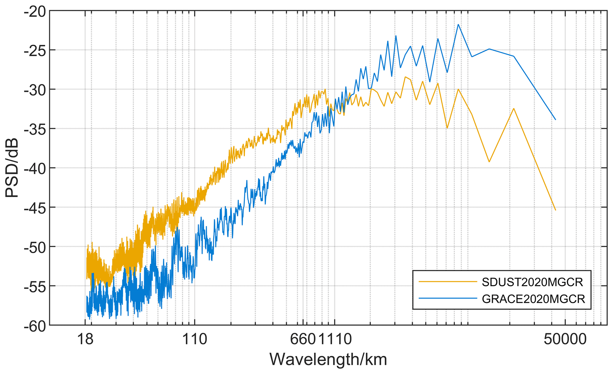
The statistical histogram of the long-term MGCR is plotted, as shown in Fig. 8. It shows that the MGCR values of SDUST2020MGCR and GRACE2020MGCR are mainly between −0.2 and 0.2 µGal yr−1, and SDUST2020MGCR is more consistent with the Gaussian normal distribution. Utilizing the periodogram method, the power spectral density of the MGCR model is estimated, and the result is illustrated in Fig. 9. The vertical axis of Fig. 9 is scaled by a factor of 10 lg; the horizontal axis is wavelength. In this study, the GRACE2020MGCR was constructed using the GRACE model of spherical harmonic degree 60. The spherical harmonic degree can be calculated from wavelength using the conversion formula 40000 divided by wavelength. Fig. 9 shows that when the wavelength exceeds 1110 km, corresponding to a spherical harmonic degree less than 36, the signal strength of GRACE2020MGCR is greater than SDUST2020MGCR. When the wavelength is greater than 660 and less than 1110 km, corresponding to a spherical harmonic degree greater than 36 and less than 60, the signal strength of GRACE2020MGCR is lower than SDUST2020MGCR, which suggests that it is possible to improve the GRACE model of spherical harmonic degree 60 by using altimetry data. When the wavelength is less than 660 km, the signal strength of SDUST2020MGCR remains greater than GRACE2020MGCR.
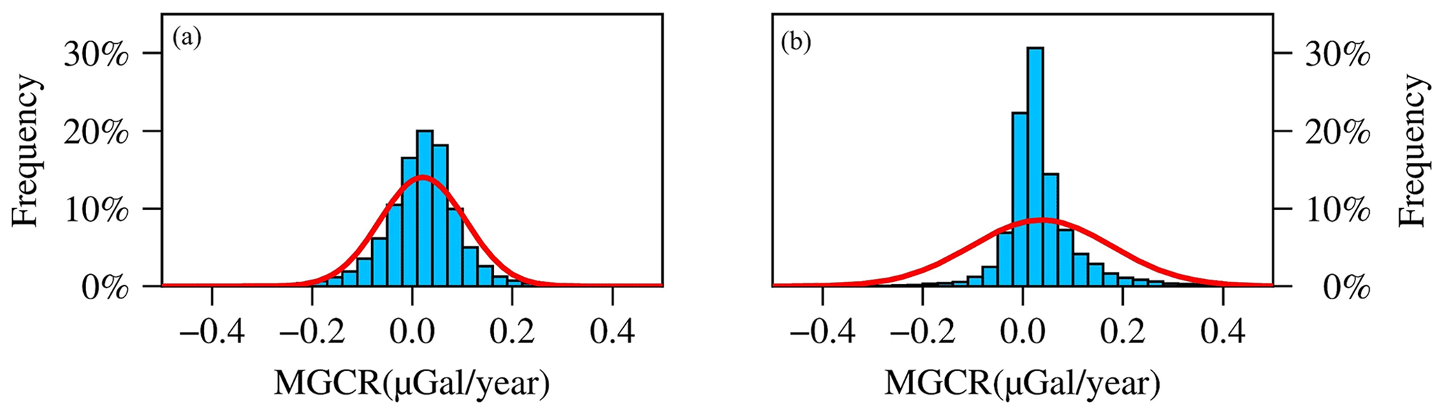
Figure 8The statistical histogram of the long-term MGCR. (a) SDUST2020MGCR; (b) GRACE2020MGCR.
There are some differences in spatial distribution and statistical results between SDUST2020MGCR and GRACE2020MGCR, which are mainly related to the following factors. (1) The spatial resolution of the GRACE/GRACE-FO monthly gravity data is low, its signal contains north–south strip noise and leakage errors, and both error correction processing and error residuals make real geophysical signals distorted and weak. (2) The satellite altimetry data exhibit relatively high spatial resolution, but its time-varying marine gravity may be affected by SSH measurement errors. (3) The EN4.2.1 ocean temperature and salinity data suffer accuracy problems that arise from irregular spatial data distribution and model gridding. Consequently, the spatial distribution and statistics of SDUST2020MGCR and GRACE2020MGCR are challenging to mutually validate.
4.3 Reliability analysis of model
In many previous studies, there is a problem that the independent observations of GRACE satellite and altimetry satellite do not match well in terms of spatial resolution and observation accuracy, the GRACE and altimetry results are difficult to verify each other (Willis et al., 2008; Feng et al., 2014). Therefore, it is not possible to use the GRACE results to assess the reliability of the altimetry results. In this study, we conducted a reliability analysis aimed at informing potential dataset users about regions where reliability is diminished.
We split the altimetry data in half, use data groups 1–5 to estimate SLCR1 and data groups 5–9 to estimate SLCR2, and then calculate the difference between the two SLCR types, and the result is depicted in Fig. 10. Where SLCR values differ substantially, the reliability of altimetry results may be reduced. The results of Fig. 10 show that the noise from altimetry observations has little effect on SLCR in most global ocean areas. The large SLCR differences are mainly observed near the ocean current areas. On the one hand, the quality of altimetry data is poor in regions with strong ocean currents (Vignudelli et al., 2006; Zhu et al., 2022), especially the West Wind Drift, and the reliability of altimetry SLCR may be low. On the other hand, global climate change leads to changes in the intensity of ocean current activities (Du et al., 2019), which objectively causes significant sea level changes near the ocean current areas. Indeed, the SLCR is estimated by applying the 19-year moving window method, which can effectively mitigate the impact of ocean currents. In summary, SLCR can overcome the influence of noise from altimetry observation to further solve the relatively stable and reliable MGCR.
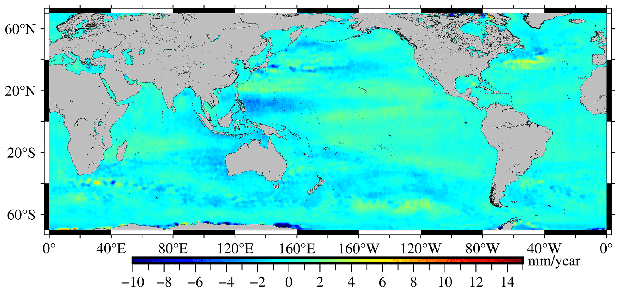
Figure 10Difference of altimetry SLCR between two periods.
The global marine gravity change rate model (SDUST2020MGCR) can be downloaded at https://doi.org/10.5281/zenodo.10701641 (Zhu et al., 2024). In this study, the GIA effect is deducted as a known factor, and thus the marine gravity change rate is investigated for other factors. In fact, many science applications that require mass change trends over the oceans would require both ocean mass signals and solid Earth effects (GIA effects and seismic deformations). Therefore, the dataset contains geospatial information (latitude, longitude), SDUST2020MGCR, and an attachment dataset (GIA MGCR). The users can sum the SDUST2020MGCR with the GIA MGCR to obtain a full-signal MGCR, or if users do not want to consider the GIA effects they can just use the SDUST2020MGCR.
This study utilized multi-satellite altimetry data and ocean temperature–salinity data from 1993 to 2019 to estimate the global mass-term SLCR. Based on the spherical harmonic function method and mass load theory, we constructed the global MGCR model (SDUST2020MGCR) on 5′ × 5′ grids. This model provides more detailed information of changes in the marine gravity field.
The SDUST2020MGCR and the GRACE/GRACE-FO global MGCR model (GRACE2020MGCR) were compared. In local sea areas where marine gravity changes significantly, such as the eastern seas of Japan, the western seas of the Nicobar Islands, and the southern seas of Greenland, the SDUST2020MGCR and GRACE2020MGCR have certain similarities in spatial distribution. However, there are some differences in the global spatial distribution between SDUST2020MGCR and GRACE2020MGCR, which is mainly related to the mismatch in spatial resolution among satellite altimetry data, satellite gravity data, and ocean temperature–salinity data. Compared with the low-resolution GRACE2020MGCR, the SDUST2020MGCR not only has a higher spatial resolution, but also excludes the strip noise and leakage errors, so it can more realistically reflect the long-term changes in the marine gravity field. The use of altimetry data can maximize the opportunity to construct a high-resolution, high-precision MGCR model. Although the altimetry MGCR may be less reliable at ocean current areas, the construction of altimetry MGCR can fill the data gap compared to the inability of GRACE to detect small-scale marine gravity changes caused by ocean currents.
The marine gravity changes are mainly caused by the seawater mass changes. (1) Global warming leads to melting of glaciers and ice sheets, sea level rise, and seawater mass increase, which in turn affect the global marine gravity field. (2) The climate warming leads to a change in ocean dynamics, such as changes in the intensity and number of tropical cyclones and enhancement of ocean circulation, which causes changes in the seawater mass distribution, and then affect the marine gravity field. (3) The variation of terrestrial water storage is unevenly distributed in space; this unevenly variation of mass will in turn load the Earth, named as self-attraction and loading effect, which causes changes in seawater mass distribution and consequently changes in marine gravity. SDUST2020MGCR has higher spatial resolution and excludes stripe noise and leakage errors; it can more realistically reflect the long-term marine gravity change in more detail, which is meaningful for the study of seawater mass migration and its associated geophysical processes.
FZ and JG designed the research and developed the algorithm. HZ downloaded altimeter data and other data. FZ carried out the experimental results and wrote the manuscript. LH, HS, and XL gave related comments for this work.
The contact author has declared that none of the authors has any competing interests.
Publisher’s note: Copernicus Publications remains neutral with regard to jurisdictional claims made in the text, published maps, institutional affiliations, or any other geographical representation in this paper. While Copernicus Publications makes every effort to include appropriate place names, the final responsibility lies with the authors.
We appreciate AVISO for providing altimeter data and monthly sea level anomaly data, the UK Met Office for contributing EN4.2.1 data, and the ICGEM for releasing GRACE/GRACE-FO monthly geopotential spherical harmonics data. Special thanks to W. Richard Peltier and Donald F. Argus for sharing the ICE-6G GIA model. Finally, we would also like to thank Generic Mapping Tools and its contributors.
This study receives partial support from the National Natural Science Foundation of China (grant nos. 42192535, 42274006, and 42242015), the Autonomous and Controllable Project for Surveying and Mapping of China (grant no. 816-517), and the Shandong University of Science and Technology Research Fund (grants no. 2014TDJH101).
This paper was edited by Alberto Ribotti and reviewed by two anonymous referees.
Andersen, O. B. and Knudsen, P.: The DTU17 Global Marine Gravity Field: First Validation Results, in: Fiducial Reference Measurements for Altimetry, Cham, 83–87, https://doi.org/10.1007/1345_2019_65, 2020.
Andersen, O. B., Abulaitijiang, A., Zhang, S., and Rose, S. K.: A new high resolution Mean Sea Surface (DTU21MSS) for improved sea level monitoring, EGU General Assembly 2021, online, 19–30 Apr 2021, EGU21-16084, https://doi.org/10.5194/egusphere-egu21-16084, 2021.
Andersen, O. B., Rose, S. K., Abulaitijiang, A., Zhang, S., and Fleury, S.: The DTU21 global mean sea surface and first evaluation, Earth Syst. Sci. Data, 15, 4065–4075, https://doi.org/10.5194/essd-15-4065-2023, 2023.
Argus, D. F., Peltier, W. R., Drummond, R., and Moore, A. W.: The Antarctica component of postglacial rebound model ICE-6G_C (VM5a) based on GPS positioning, exposure age dating of ice thicknesses, and relative sea level histories, Geophys. J. Int., 198, 537–563, https://doi.org/10.1093/gji/ggu140, 2014.
Cazenave, A., Dieng, H.-B., Meyssignac, B., Von Schuckmann, K., Decharme, B., and Berthier, E.: The rate of sea-level rise, Nat. Clim. Change, 4, 358–361, https://doi.org/10.1038/nclimate2159, 2014.
Chen, J., Li, J., Zhang, Z., and Ni, S.: Long-term groundwater variations in Northwest India from satellite gravity measurements, Global Planet. Change, 116, 130–138, https://doi.org/10.1016/j.gloplacha.2014.02.007, 2014.
CNES: Along-track Level-2+ (L2P) SLA Product Handbook, SALP-MU-P-EA-23150-CLS, Issue 2.0, https://www.aviso.altimetry.fr/fileadmin/documents/data/tools/hdbk_L2P_all_missions_except_S3.pdf (last access: 6 November 2023), 2020.
Du, Y., Zhang, Y., and Shi, J.: Relationship between sea surface salinity and ocean circulation and climate change, Sci. China Earth Sci., 62, 771–782, https://doi.org/10.1007/s11430-018-9276-6, 2019.
Ducet, N., Le Traon, P. Y., and Reverdin, G.: Global high-resolution mapping of ocean circulation from TOPEX/Poseidon and ERS-1 and -2, J. Geophys. Res., 105, 19477–19498, https://doi.org/10.1029/2000JC900063, 2000.
Feng, W., Zhong, M., and Xu, H.: Global sea level changes estimated from satellite altimetry, satellite gravimetry and Argo data during 2005–2013, Prog. Geophys., 29, 471–477, 2014.
Flechtner, F., Reigber, C., Rummel, R., and Balmino, G.: Satellite Gravimetry: A Review of Its Realization, Surv. Geophys., 42, 1029–1074, https://doi.org/10.1007/s10712-021-09658-0, 2021.
Flury, J. and Rummel, R. (Eds.): Future satellite gravimetry and earth dynamics, Springer, Dordrecht, 163 pp., https://doi.org/10.1007/0-387-33185-9, 2005.
Fofonoff, N. and Millard, R.: Algorithms for computation of fundamental properties of seawater, in: UNESCO technical papersin marine science, Ocean best practices, 44, https://doi.org/10.25607/OBP-1450, 1983.
Godah, W.: IGiK–TVGMF: A MATLAB package for computing and analysing temporal variations of gravity/mass functionals from GRACE satellite based global geopotential models, Comput. Geosci., 123, 47–58, https://doi.org/10.1016/j.cageo.2018.11.008, 2019.
Good, S. A., Martin, M. J., and Rayner, N. A.: EN4: Quality controlled ocean temperature and salinity profiles and monthly objective analyses with uncertainty estimates: THE EN4 DATA SET, J. Geophys. Res.-Oceans, 118, 6704–6716, https://doi.org/10.1002/2013JC009067, 2013.
Gopalapillai, G. S. and Mourad, A. G.: Detailed gravity anomalies from Geos 3 satellite altimetry data, J. Geophys. Res., 84, 6213–6218, https://doi.org/10.1029/JB084iB11p06213, 1979.
Greco, F., Currenti, G., D'Agostino, G., Germak, A., Napoli, R., Pistorio, A., and Del Negro, C.: Combining relative and absolute gravity measurements to enhance volcano monitoring, Bull. Volcanol., 74, 1745–1756, https://doi.org/10.1007/s00445-012-0630-0, 2012.
Groh, A., Horwath, M., Horvath, A., Meister, R., Sørensen, L. S., Barletta, V. R., Forsberg, R., Wouters, B., Ditmar, P., Ran, J., Klees, R., Su, X., Shang, K., Guo, J., Shum, C. K., Schrama, E., and Shepherd, A.: Evaluating GRACE Mass Change Time Series for the Antarctic and Greenland Ice Sheet – Methods and Results, Geosciences, 9, 415, https://doi.org/10.3390/geosciences9100415, 2019.
Han, S.-C., Jekeli, C., and Shum, C. K.: Time-variable aliasing effects of ocean tides, atmosphere, and continental water mass on monthly mean GRACE gravity field: Temporal Aliasing on GRACE Gravity Field, J. Geophys. Res., 109, B04403, https://doi.org/10.1029/2003JB002501, 2004.
Hosoda, S., Ohira, T., and Nakamura, T.: A monthly mean dataset of global oceanic temperature and salinity derived from Argo float observations, JAMSTEC-R, 8, 47–59, https://doi.org/10.5918/jamstecr.8.47, 2008.
Huang, M., Zhai, G., Ouyang, Y., Lu, X., Liu, C., and Wang, R.: Integrated Data Processing for Multi-Satellite Missions and Recovery of Marine Gravity Field, Terr. Atmos. Ocean. Sci., 19, 103–109, https://doi.org/10.3319/TAO.2008.19.1-2.103(SA), 2008.
Hwang, C., Hsu, H.-Y., and Jang, R.-J.: Global mean sea surface and marine gravity anomaly from multi-satellite altimetry: applications of deflection-geoid and inverse Vening Meinesz formulae, J. Geodesy, 76, 407–418, https://doi.org/10.1007/s00190-002-0265-6, 2002.
Jin, T., Li, J., Jiang, W., and Wang, Z.: The new generation of global mean sea surface height model based on multi-altimetric data, Acta Geodaetica et Cartographica Sinica, 40, 723–729, 2011.
Jordan, S. K.: Self-consistent statistical models for the gravity anomaly, vertical deflections, and undulation of the geoid, J. Geophys. Res., 77, 3660–3670, https://doi.org/10.1029/JB077i020p03660, 1972.
Kusche, J.: Approximate decorrelation and non-isotropic smoothing of time-variable GRACE-type gravity field models, J. Geodesy, 81, 733–749, https://doi.org/10.1007/s00190-007-0143-3, 2007.
Leuliette, E. W. and Miller, L.: Closing the sea level rise budget with altimetry, Argo, and GRACE, Geophys. Res. Lett., 36, 2008GL036010, https://doi.org/10.1029/2008GL036010, 2009.
Li, Q., Bao, L., and Shum, C. K.: Altimeter-derived marine gravity variations reveal the magma mass motions within the subaqueous Nishinoshima volcano, Izu–Bonin Arc, Japan, J. Geodesy, 95, 46, https://doi.org/10.1007/s00190-021-01488-7, 2021.
Liang, W., Zhang, G., Zhu, Y., Xu, Y., Guo, S., Zhao, Y., Liu, F., and Zhao, L.: Gravity variations before the Menyuan Ms 6.4 earthquake, Geodesy and Geodynamics, 7, 223–229, https://doi.org/10.1016/j.geog.2016.04.013, 2016.
Llovel, W., Guinehut, S., and Cazenave, A.: Regional and interannual variability in sea level over 2002–2009 based on satellite altimetry, Argo float data and GRACE ocean mass, Ocean Dynam., 60, 1193–1204, https://doi.org/10.1007/s10236-010-0324-0, 2010.
Nerem, R. S., Chambers, D. P., Choe, C., and Mitchum, G. T.: Estimating Mean Sea Level Change from the TOPEX and Jason Altimeter Missions, Mar. Geod., 33, 435–446, https://doi.org/10.1080/01490419.2010.491031, 2010.
Peltier, W. R., Argus, D. F., and Drummond, R.: Space geodesy constrains ice age terminal deglaciation: The global ICE-6G_C (VM5a) model, J. Geophys. Res.-Sol. Ea., 120, 450–487, https://doi.org/10.1002/2014JB011176, 2015.
Rapp, R. H., Yi, Y., and Wang, Y. M.: Mean sea surface and geoid gradient comparisons with TOPEX altimeter data, J. Geophys. Res., 99, 24657–24667, https://doi.org/10.1029/94JC00918, 1994.
Riser, S. C., Freeland, H. J., Roemmich, D., Wijffels, S., Troisi, A., Belbéoch, M., Gilbert, D., Xu, J., Pouliquen, S., Thresher, A., Le Traon, P.-Y., Maze, G., Klein, B., Ravichandran, M., Grant, F., Poulain, P.-M., Suga, T., Lim, B., Sterl, A., Sutton, P., Mork, K.-A., Vélez-Belchí, P. J., Ansorge, I., King, B., Turton, J., Baringer, M., and Jayne, S. R.: Fifteen years of ocean observations with the global Argo array, Nat. Clim. Change, 6, 145–153, https://doi.org/10.1038/nclimate2872, 2016.
Roemmich, D. and Gilson, J.: The 2004–2008 mean and annual cycle of temperature, salinity, and steric height in the global ocean from the Argo Program, Prog. Oceanogr., 82, 81–100, https://doi.org/10.1016/j.pocean.2009.03.004, 2009.
Sandwell, D., Garcia, E., Soofi, K., Wessel, P., Chandler, M., and Smith, W. H. F.: Toward 1-mGal accuracy in global marine gravity from CryoSat-2, Envisat, and Jason-1, The Leading Edge, 32, 892–899, https://doi.org/10.1190/tle32080892.1, 2013.
Sandwell, D. T., Harper, H., Tozer, B., and Smith, W. H. F.: Gravity field recovery from geodetic altimeter missions, Adv. Space Res., 68, 1059–1072, https://doi.org/10.1016/j.asr.2019.09.011, 2021.
Schaeffer, P., Faugére, Y., Legeais, J. F., Ollivier, A., Guinle, T., and Picot, N.: The CNES_CLS11 Global Mean Sea Surface Computed from 16 Years of Satellite Altimeter Data, Mar. Geod., 35, 3–19, https://doi.org/10.1080/01490419.2012.718231, 2012.
Sneeuw, N.: Global spherical harmonic analysis by least-squares and numerical quadrature methods in historical perspective, Geophys. J. Int., 118, 707–716, https://doi.org/10.1111/j.1365-246X.1994.tb03995.x, 1994.
Sun, Y., Riva, R., Ditmar, P., and Rietbroek, R.: Using GRACE to Explain Variations in the Earth's Oblateness, Geophys. Res. Lett., 46, 158–168, https://doi.org/10.1029/2018GL080607, 2019.
Taburet, G., Sanchez-Roman, A., Ballarotta, M., Pujol, M.-I., Legeais, J.-F., Fournier, F., Faugere, Y., and Dibarboure, G.: DUACS DT2018: 25 years of reprocessed sea level altimetry products, Ocean Sci., 15, 1207–1224, https://doi.org/10.5194/os-15-1207-2019, 2019.
Tamisiea, M. E., Hill, E. M., Ponte, R. M., Davis, J. L., Velicogna, I., and Vinogradova, N. T.: Impact of self-attraction and loading on the annual cycle in sea level, J. Geophys. Res., 115, 2009JC005687, https://doi.org/10.1029/2009JC005687, 2010.
Tapley, B. D., Bettadpur, S., Ries, J. C., Thompson, P. F., and Watkins, M. M.: GRACE Measurements of Mass Variability in the Earth System, Science, 305, 503–505, https://doi.org/10.1126/science.1099192, 2004.
UTCSR: Gravity Recovery and Climate Experiment UTCSR Level-2 processing standards document, Issue5.0, https://archive.podaac.earthdata.nasa.gov/podaac-ops-cumulus-docs/grace/open/docs/L2-CSR006_ProcStd_v5.0.pdf (last access: 6 November 2023), 2018.
Vignudelli, S., Snaith, H. M., Lyard, F., Cipollini, P., Venuti, F., Birol, F., Bouffard, J., and Roblou, L.: Satellite radar altimetry from open ocean to coasts: challenges and perspectives, Asia-Pacific Remote Sensing Symposium, Goa, India, 28 November 2006, 64060L, https://doi.org/10.1117/12.694024, 2006.
Wahr, J., Molenaar, M., and Bryan, F.: Time variability of the Earth's gravity field: Hydrological and oceanic effects and their possible detection using GRACE, J. Geophys. Res., 103, 30205–30229, https://doi.org/10.1029/98JB02844, 1998.
Wahr, J., Swenson, S., Zlotnicki, V., and Velicogna, I.: Time-variable gravity from GRACE: First results: TIME-VARIABLE GRAVITY FROM GRACE, Geophys. Res. Lett., 31, L11501, https://doi.org/10.1029/2004GL019779, 2004.
Wang, Y.-L. and Wu, C.-R.: Enhanced Warming and Intensification of the Kuroshio Extension, 1999–2013, Remote Sensing, 11, 101, https://doi.org/10.3390/rs11010101, 2019.
Willis, J. K., Chambers, D. P., and Nerem, R. S.: Assessing the globally averaged sea level budget on seasonal to interannual timescales, J. Geophys. Res., 113, C06015, https://doi.org/10.1029/2007JC004517, 2008.
Wouters, B., Bonin, J. A., Chambers, D. P., Riva, R. E. M., Sasgen, I., and Wahr, J.: GRACE, time-varying gravity, Earth system dynamics and climate change, Rep. Prog. Phys., 77, 116801, https://doi.org/10.1088/0034-4885/77/11/116801, 2014.
Yang, Y., Feng, W., Zhong, M., Mu, D., and Yao, Y.: Basin-Scale Sea Level Budget from Satellite Altimetry, Satellite Gravimetry, and Argo Data over 2005 to 2019, Remote Sensing, 14, 4637, https://doi.org/10.3390/rs14184637, 2022.
Yuan, J., Guo, J., Liu, X., Zhu, C., Niu, Y., Li, Z., Ji, B., and Ouyang, Y.: Mean sea surface model over China seas and its adjacent ocean established with the 19-year moving average method from multi-satellite altimeter data, Cont. Shelf Res., 192, 104009, https://doi.org/10.1016/j.csr.2019.104009, 2020a.
Yuan, J., Guo, J., Niu, Y., Zhu, C., and Li, Z.: Mean Sea Surface Model over the Sea of Japan Determined from Multi-Satellite Altimeter Data and Tide Gauge Records, Remote Sensing, 12, 4168, https://doi.org/10.3390/rs12244168, 2020b.
Yuan, J., Guo, J., Zhu, C., Hwang, C., Yu, D., Sun, M., and Mu, D.: High-resolution sea level change around China seas revealed through multi-satellite altimeter data, Int. J. Appl. Earth Obs., 102, 102433, https://doi.org/10.1016/j.jag.2021.102433, 2021.
Yuan, J., Guo, J., Zhu, C., Li, Z., Liu, X., and Gao, J.: SDUST2020 MSS: a global 1′ × 1′ mean sea surface model determined from multi-satellite altimetry data, Earth Syst. Sci. Data, 15, 155–169, https://doi.org/10.5194/essd-15-155-2023, 2023.
Zhang, S., Abulaitijiang, A., Andersen, O. B., Sandwell, D. T., and Beale, J. R.: Comparison and evaluation of high-resolution marine gravity recovery via sea surface heights or sea surface slopes, J. Geodesy, 95, 66, https://doi.org/10.1007/s00190-021-01506-8, 2021.
Zhu, C., Guo, J., Yuan, J., Li, Z., Liu, X., and Gao, J.: SDUST2021GRA: global marine gravity anomaly model recovered from Ka-band and Ku-band satellite altimeter data, Earth Syst. Sci. Data, 14, 4589–4606, https://doi.org/10.5194/essd-14-4589-2022, 2022.
Zhu, F., Liu, X., Li, Z., Yuan, J., Guo, J., and Sun, H.: High spatial resolution marine gravity trend determined from multisatellite altimeter data over Bay of Bengal, Geophys. J. Int., 235, 2257–2267, https://doi.org/10.1093/gji/ggad368, 2023.
Zhu, F., Guo, J., Zhang, H., Huang, L., Sun, H., and Liu, X.: SDUST2020MGCR: a global marine gravity change rate model determined from multi-satellite altimeter data, Zenodo [data set], https://doi.org/10.5281/zenodo.10701641, 2024.