the Creative Commons Attribution 4.0 License.
the Creative Commons Attribution 4.0 License.
 | 12 Apr 2024
CAMELE: Collocation-Analyzed Multi-source Ensembled Land Evapotranspiration Data
Changming Li
Ziwei Liu
Wencong Yang
Zhuoyi Tu
Juntai Han
Sien Li
Land evapotranspiration (ET) plays a crucial role in Earth's water–carbon cycle, and accurately estimating global land ET is vital for advancing our understanding of land–atmosphere interactions. Despite the development of numerous ET products in recent decades, widely used products still possess inherent uncertainties arising from using different forcing inputs and imperfect model parameterizations. Furthermore, the lack of sufficient global in situ observations makes direct evaluation of ET products impractical, impeding their utilization and assimilation. Therefore, establishing a reliable global benchmark dataset and exploring evaluation methodologies for ET products is paramount. This study aims to address these challenges by (1) proposing a collocation-based method that considers non-zero error cross-correlation for merging multi-source data and (2) employing this merging method to generate a long-term daily global ET product at resolutions of 0.1° (2000–2020) and 0.25° (1980–2022), incorporating inputs from ERA5L, FluxCom, PMLv2, GLDAS, and GLEAM. The resulting product is the Collocation-Analyzed Multi-source Ensembled Land Evapotranspiration Data (CAMELE). CAMELE exhibits promising performance across various vegetation coverage types, as validated against in situ observations. The evaluation process yielded Pearson correlation coefficients (R) of 0.63 and 0.65, root-mean-square errors (RMSEs) of 0.81 and 0.73 mm d−1, unbiased root-mean-square errors (ubRMSEs) of 1.20 and 1.04 mm d−1, mean absolute errors (MAEs) of 0.81 and 0.73 mm d−1, and Kling–Gupta efficiencies (KGEs) of 0.60 and 0.65 on average at resolutions of 0.1 and 0.25°, respectively. In addition, comparisons indicate that CAMELE can effectively characterize the multiyear linear trend, mean average, and extreme values of ET. However, it exhibits a tendency to overestimate seasonality. In summary, we propose a reliable set of ET data that can aid in understanding the variations in the water cycle and has the potential to serve as a benchmark for various applications. The dataset is publicly available at https://doi.org/10.5281/zenodo.8047038 (Li et al., 2023b).
- Article
(30884 KB) - Full-text XML
-
Supplement
(1039 KB) - BibTeX
- EndNote


Land evapotranspiration (ET) plays a critical role in the global water and energy cycles, encompassing various processes such as soil evaporation, vegetation transpiration, canopy interception, and surface water evaporation (Zhang et al., 2019; Zhao et al., 2022; Lian et al., 2018). Accurately estimating global land evapotranspiration is vital for understanding the hydrological cycle and land–atmosphere interactions, as it serves as an intermediary variable connecting soil moisture, air temperature, and humidity (Miralles et al., 2019; Gentine et al., 2019). Therefore, providing a reliable ET dataset as a benchmark for further research is crucial.
In recent decades, numerous studies have focused on estimating global land evapotranspiration, resulting in many datasets (Yang et al., 2023). However, discrepancies often arise among these simulations due to algorithm and principle variations (Restrepo-Coupe et al., 2021; Han and Tian, 2020). Additionally, evaluating ET products is challenging due to the limited availability of global-scale observations, which hampers their direct use (Pan et al., 2020; Baker et al., 2021).
The fusion of multi-source data is a suitable option for addressing these uncertainties. Recent studies have explored several approaches to integrate multiple ET products, including simple averaging (SA) (Ershadi et al., 2014), Bayesian model averaging (BMA) (Hao et al., 2019; Ma et al., 2020; Zhu et al., 2016), reliability ensemble averaging (REA) (Lu et al., 2021), empirical orthogonal functions (EOFs) (Feng et al., 2016), and machine-learning-based methods (Chen et al., 2020; Yin et al., 2021). However, the primary challenge lies in calculating reliable input weights based on a selected “truth” (Koster et al., 2021), which can involve averaging or incorporating other relevant geographical information as a benchmark.
Recently, collocation methods have emerged as promising techniques for estimating random error variances and data–truth correlations in collocated inputs (Stoffelen, 1998; Li et al., 2022; X. Li et al., 2023; Park et al., 2023). These methods consider the errors associated with collocated datasets as an accurate representation of uncertainty without assuming the absence of errors in any datasets. It is important to note that while collocation methods, such as the triple collocation (TC) and the extended double instrumental variable technique (EIVD), can estimate the variance (or covariance) of random errors, they cannot evaluate the bias of the products. One primary advantage of collocation analysis is that it does not require a high-quality reference dataset (Su et al., 2014; Wu et al., 2021). However, a crucial prerequisite for applying collocation methods is the availability of many spatially and temporally corresponding datasets. For instance, the classic TC method requires a trio of independent datasets. Su et al. (2014) used the instrumental regression method and considered lag-1 time series as the third input, proposing the single instrumental variable algorithm (IVS). Dong et al. (2019) introduced the lag-1 time series from both inputs, proposing the double instrumental variable algorithm (IVD) for a more robust solution. Gruber et al. (2016a) extended the original algorithm to incorporate more datasets, partially addressing the independence assumption to calculate a portion of error cross-correlation (ECC) by using the extended collocation (EC) method. Dong et al. (2020a) further proposed the EIVD method, enabling ECC estimation using three datasets. Collocation methods have found widespread application in the evaluation of geophysical variable estimates, including soil moisture (Deng et al., 2023; Ming et al., 2022), precipitation (Dong et al., 2022; Li et al., 2018), ocean wind speed (Vogelzang et al., 2022; Ribal and Young, 2020), leaf area index (Jiang et al., 2017), total water storage (Yin and Park, 2021), sea ice thickness and surface salinity (Hoareau et al., 2018), and near-surface air temperature (Sun et al., 2021).
Recently, many studies have utilized collocation approaches to evaluate evapotranspiration products, with the TC method to assess uncertainties. For example, Barraza Bernadas et al. (2018) considered the uncertainties of ET from the Breathing Earth System Simulator, BESS (Jiang et al., 2020; Jiang and Ryu, 2016), Moderate Resolution Imaging Spectroradiometer, MOD16 (Mu et al., 2011), and a hybrid model; Khan et al. (2018) utilized extended triple collocation (ETC) (McColl et al., 2014) to investigate the reliability of ET from MOD16, the Global Land Data Assimilation System (GLDAS) (Rodell et al., 2004), and the Global Land Evaporation Amsterdam Model (GLEAM) (Martens et al., 2017) over East Asia; Li et al. (2022) employed five collocation methods (i.e., IVS, IVD, TC, EIVD, and EC) to analyze the uncertainties of ET from ERA5-Land (ERA5L) (Muñoz-Sabater et al., 2021), GLEAM, GLDAS, FluxCom (Jung et al., 2019), and the Penman–Monteith–Leuning evapotranspiration V2 (PMLv2) (Zhang et al., 2019).
Moreover, error information derived from collocation analysis is valuable for merging multi-source data. This was initially applied by Yilmaz et al. (2012) in the fusion of multi-source soil moisture products and later improved by Gruber et al. (2017) and further applied in the production of the European Space Agency Climate Change Initiative (ESA CCI) global soil moisture product (Gruber et al., 2019). Dong et al. (2020b) also adopted this approach to fusing multi-source precipitation products. In the study of evapotranspiration, X. Li et al. (2023) and Park et al. (2023) utilized a weight calculation method that does not consider non-zero ECC and fused multiple ET products in Nordic and East Asia, respectively, achieving satisfactory fusion results.
Although the above studies have demonstrated that collocation analysis can effectively assess the random error variance of ET products and integrate error information from multiple data sources, these studies have primarily overlooked a critical aspect: non-zero ECC between ET products. Li et al. (2022) global ET product evaluation research revealed clear non-zero ECC conditions between ERA5L, GLEAM, PMLv2, and FluxCom. In TC analysis, non-zero ECC can result in significant biases in TC-based results (Yilmaz and Crow, 2014). Furthermore, when using TC-based error information for fusion, it is crucial to consider the information related to ECC, as this can help improve the fusion accuracy (Dong et al., 2020b; Kim et al., 2021b).
It is worth noting that non-zero ECC conditions pose unique challenges. Unlike other violations of mathematical assumptions adopted by TC, they cannot be effectively mitigated through rescaling or compensated for by equal-magnitude adjustments across inputs. Thus, the implications of non-zero ECC in the context of merging strategies are a critical consideration often overlooked in previous research. This oversight can lead to significant biases and inaccuracies. We aim to bridge this gap by systematically accounting for non-zero ECC in weight calculation, contributing to a more robust and accurate assessment.
In this study, we propose a collocation-based data ensemble method, considering non-zero ECC conditions, for merging multiple ET products to create the Collocation-Analyzed Multi-source Ensembled Land Evapotranspiration data, abbreviated as CAMELE. The second section of this paper presents the selected data information. In the third section, we explain the error calculation method for collocation analysis and the weighted calculation method that considered ECC. The fourth section analyzes the global errors of different ET products obtained through these calculations and the distribution patterns of the corresponding weights. We evaluate the accuracy of the fused products and compare them with existing products using reference values from site measurements. In the fifth section, we discuss the inherent errors in the methods, analyze the ECC between the products, and compare the differences between the different fusion schemes. Finally, in the sixth section, we summarize the results obtained from this research.
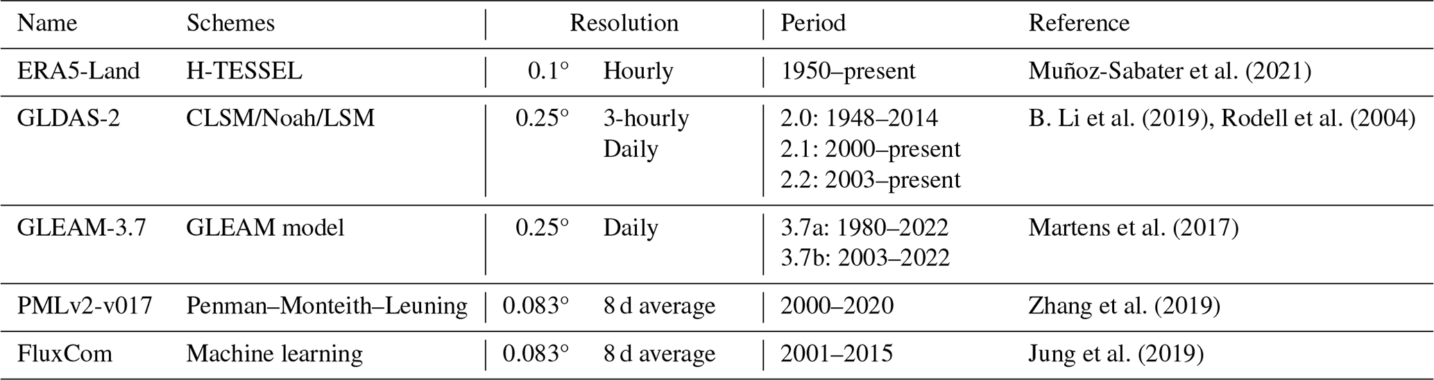
We selected five widely used ET products that spanned the period from 1980 to 2022. When selecting these products, our aims are to ensure (1) consistency in the original spatiotemporal resolution among the products: minimize potential downscaling operations and avoid introducing additional errors; (2) three or more products within the same resolution or period: incorporate more information for effective fusion; and (3) products with extensive global observational sequences: gain basic recognition from the community. While we acknowledge the existence of other higher-precision products, their integration would require either downscaling or upscaling of other products, potentially introducing uncertainties. Therefore, we chose the combination outlined in the paper. Despite its relatively lower resolution compared to some products, it still contributes to our understanding of ET variations, facilitating advantageous exploration. Furthermore, we incorporated in situ observations and the Lu et al. (2021) global 0.25° daily-scale ET product derived using REA to compare our merged product comprehensively. Table 1 shows the spatial and temporal resolutions of the input datasets.
2.1 ERA5-Land
The European Centre for Medium-Range Weather Forecasts (ECMWF) produces the latest advanced ERA5L, a global hourly reanalysis dataset with a spatial resolution of 0.1°. It covers the period from January 1950 until approximately 1 week before the present (Muñoz-Sabater et al., 2021). ERA5-Land is derived from the land component of the ECMWF climate reanalysis, incorporating numerous improvements over previously released versions. It is based on the Tiled ECMWF Scheme for Surface Exchanges over Land incorporating land surface hydrology (H-TESSEL), utilizing version CY45R1 of the ECMWF's Integrated Forecasting System (IFS). The dataset benefits from atmospheric forcing data, which acts as an indirect constraint on the model-based estimates (Hersbach et al., 2020). The dataset is available through the Climate Change service of the Copernicus Center at https://cds.climate.copernicus.eu/cdsapp#!/dataset/reanalysis-era5-land?tab=overview (last access: 10 April 2024).
Evapotranspiration in ERA5L, defined as “total evaporation”, represents the accumulated amount of water that has evaporated from the Earth's surface, including a simplified representation of transpiration from vegetation into the vapor in the air. The soil water and energy balance are computed using standard soil discretization. Readers could consult Sect. 8.6.5 of the IFS documentation (ECMWF, 2014). The original dataset is interpolated from (1801, 3600) to (1800, 3600) using kriging interpolation and then upscaled from an hourly to a daily resolution, changing the spatial resolution from 0.1 to 0.25°.
2.2 GLDAS
The GLDAS product utilizes advanced data assimilation methodologies, integrating model and observation datasets for land-surface simulations (Rodell et al., 2004). GLDAS employs multiple land-surface models (LSMs), i.e., Noah, Mosaic, Variable Infiltration Capacity (VIC), and the Community Land Model (CLM). Together, these models generate global evapotranspiration estimates at fine and coarse spatial resolutions (0.01 and 0.25°) and temporal resolutions (3-hourly and monthly). The most recent iteration of GLDAS, version 2, consists of three components: GLDAS-2.0, GLDAS-2.1, and GLDAS-2.2. GLDAS-2.0 relies entirely on the Princeton meteorological forcing input data, providing a consistent temporal series from 1948 to 2014 (Sheffield et al., 2006). The GLDAS-2.1 simulation commences on 1 January 2000, utilizing the conditions from the GLDAS-2.0 simulation. On the other hand, GLDAS-2.2 is simulated from 1 February 2003, employing the conditions from GLDAS-2.0 and forcing with meteorological analysis fields from the ECMWF IFS. Additionally, the GRACE satellite's total terrestrial water anomaly observation is assimilated into the GLDAS-2.2 product (B. Li et al., 2019).
This study aimed to cover the research period from 1980 to 2022. Non-zero ECC between the transpiration estimates of GLDAS-2.2 and ERA5L was reported in a recent study (Li et al., 2023a). Considering the similarities in the calculation of ET and transpiration of GLDAS and ERA5L, this report partially indicates a correlation. Therefore, GLDAS-2.0 and GLDAS-2.1 were selected as inputs instead. The “Evap_tavg” parameter representing evapotranspiration is derived from the original products and aggregated to a daily scale. For more detailed information on the GLDAS-2 models, please refer to NASA's Hydrology Data and Information Services Center at https://disc.gsfc.nasa.gov/datasets?keywords=GLDAS (last access: 10 April 2024).
Despite the same forcing between GLDAS-2.1 and GLDAS-2.2, significant differences exist between the model results of different GLDAS versions (Qi et al., 2020, 2018; Jiménez et al., 2011). The non-zero ECC will generally still be met between different versions. Thus, we still need to analyze the non-zero ECC situations between ERA5L and GLDAS-2.0 and GLDAS-2.1, which will be assessed in the Discussion section.
2.3 Global Land Evaporation Amsterdam Model 3.7 (GLEAM-3.7)
The version of the GLEAM-3.7 dataset (Martens et al., 2017; Miralles et al., 2011) at 0.25° is used. This version of GLEAM provides daily estimations of actual evaporation, bare soil evaporation, canopy interception, transpiration from vegetation, potential evaporation, and snow sublimation. The third version of GLEAM contains a new DA scheme, an updated water balance module, and evaporative stress functions. Two datasets that differ only in forcing and temporal coverage are provided: GLEAMv3.7a 43-year period (1980 to 2022) based on satellite and reanalysis (ECMWF) data and GLEAMv3.7b 20-year period (2003 to 2022) based only on satellite data. GLEAMv3.7a is used in this study. The data are freely available on the GLEAM website (https://www.gleam.eu, last access: 10 April 2024).
The cover-dependent potential evaporation rate (EP) is calculated using the Priestley–Taylor equation (Priestley and Taylor, 1972). Then, a multiplicative stress factor is used to convert EP into actual transpiration and bare soil evaporation, which is a function of microwave vegetation optimal depth (VOD) and root-zone soil moisture. For a detailed description, please refer to the paper by Martens et al. (2017). The GLEAM data were validated at 43 FluxNet flux sites and have been proven to provide reliable ET estimations (Majozi et al., 2017).
2.4 Penman–Monteith–Leuning version 2 global evaporation model (PMLv2)
PMLv2 has been developed based on the Penman–Monteith–Leuning model (Zhang et al., 2019; Leuning et al., 2008). Initially proposed by Leuning et al. (2008), the PML model underwent further enhancements by Zhang et al. (2010). The PML version 1 (PMLv1) incorporates a biophysical model that considers canopy physiological processes and soil evaporation to estimate surface conductance accurately (Gs), which is the focus of the PM-based method. This version was subsequently enhanced by incorporating a canopy conductance (Gc) model that couples vegetation transpiration with gross primary productivity, resulting in the development of PMLv2 as described by Gan et al. (2018). Zhang et al. (2019) applied the PMLv2 model globally. The daily inputs for this model include leaf area index (LAI), broadband albedo, and emissivity obtained from the Moderate Resolution Imaging Spectroradiometer (MODIS) as well as temperature variables (daily maximum temperature – Tmax, daily minimum temperature – Tmin, daily mean temperature – Tavg), instantaneous variables (surface pressure – Psurf, atmosphere pressure – Pa, wind speed at 10 m height – U, specific humidity – q), and accumulated variables (precipitation – Prcp, inward longwave solar radiation – Rln, inward shortwave solar radiation – Rs) from GLDAS-2.0. Evaporation is divided into direct evaporation from bare soil (Es), evaporation from solid water sources (water bodies, snow, and ice) (ETwater), and vegetation transpiration (Ec). To ensure its accuracy, the PMLv2 ET model was calibrated against 8-daily eddy covariance data from 95 global flux towers representing 10 different land cover types.
In this study, we employ the latest version, v017. The data are freely available through Google Earth Engine (https://developers.google.com/earth-engine/datasets/catalog/CAS_IGSNRR_PML_V2_v017, last access: 10 April 2024).
2.5 FluxCom
FluxCom is a machine-learning-based approach combining global land–atmosphere energy flux data by combining remote sensing and meteorological data (Jung et al., 2019). To achieve this, FluxCom utilizes various machine-learning regression tools, including tree-based methods, regression splines, neural networks, and kernel methods. The outputs of FluxCom are designed based on two complementary strategies: (1) FluxCom-RS, which exclusively merges remote sensing data to generate high-spatial-resolution flux data; and (2) FluxCom-RS+METEO, which combines meteorological observations with remote sensing data at a daily temporal resolution. The exclusive use of remote sensing data in the ensemble allows production of gridded flux products at a spatial resolution of 500 m, albeit with a relatively low frequency of 8 d. It is important to note that the FluxCom-RS data only cover the period after 2000 due to data availability.
In contrast, the merging of meteorological and remote sensing data extends the coverage back to 1980 at the cost of a coarser spatial resolution of 0.5°. For more detailed information about the FluxCom dataset, please refer to the FluxCom website (http://FluxCom.org/, last access: 10 April 2024). The data are freely available by contacting the authors.
In this study, we utilized the FluxCom-RS 8-daily 0.0833° energy flux data and converted the latent heat values to evapotranspiration using ERA5L-aggregated daily air temperature. Furthermore, the original ET data were interpolated to a spatial resolution of 0.1° using the MATLAB Gaussian process regression package.
2.6 Global in situ observation: FluxNet
The latest FluxNet2015 4.0 eddy covariance data were used in our study (Pastorello et al., 2020). Following the filtering process by Lin et al. (2018) and X. Li et al. (2019), firstly, only the measured and good-quality gap-filled data were used for quality control. Secondly, we excluded days with rainfall and the subsequent day after rainy events to mitigate the impact of canopy interception (Medlyn et al., 2017; Knauer et al., 2018). Additionally, previous studies have indicated an energy imbalance problem in FluxNet2015 data. Therefore, following the method proposed by Twine et al. (2000), the measured ET data were corrected using the residual method based on energy balance.
After data filtering and processing, 212 sites are selected as shown in Fig. 1. The selected sites are distributed globally, primarily in North America and Europe. The International-Geosphere–Biosphere Program (IGBP) land cover classification system (Loveland et al., 1999) was employed to distinguish the 13 plant functional types (PFTs) across sites. The IGBP classification was determined based on metadata from the FluxNet official website, including evergreen needleleaf forests (ENF, 49 sites), evergreen broadleaf forests (EBF, 15 sites), deciduous broadleaf forests (DBF, 26 sites), croplands (CRO, 20 sites), grasslands (GRA, 39 sites), savannas (SAV, 9 sites), mixed forests (MF, 9 sites), closed shrublands (CSH, 3 sites), deciduous needleleaf forests (DNF, 1 site), open shrublands (OSH, 13 sites), snow and ice (SNO, 1 site), woody savannas (WSA, 6 sites), and permanent wetlands (WET, 21 sites). Changes in the IGBP classification during the study period are possible, but such information is not publicly available. Interested parties can obtain relevant information by directly contacting the site coordinators.
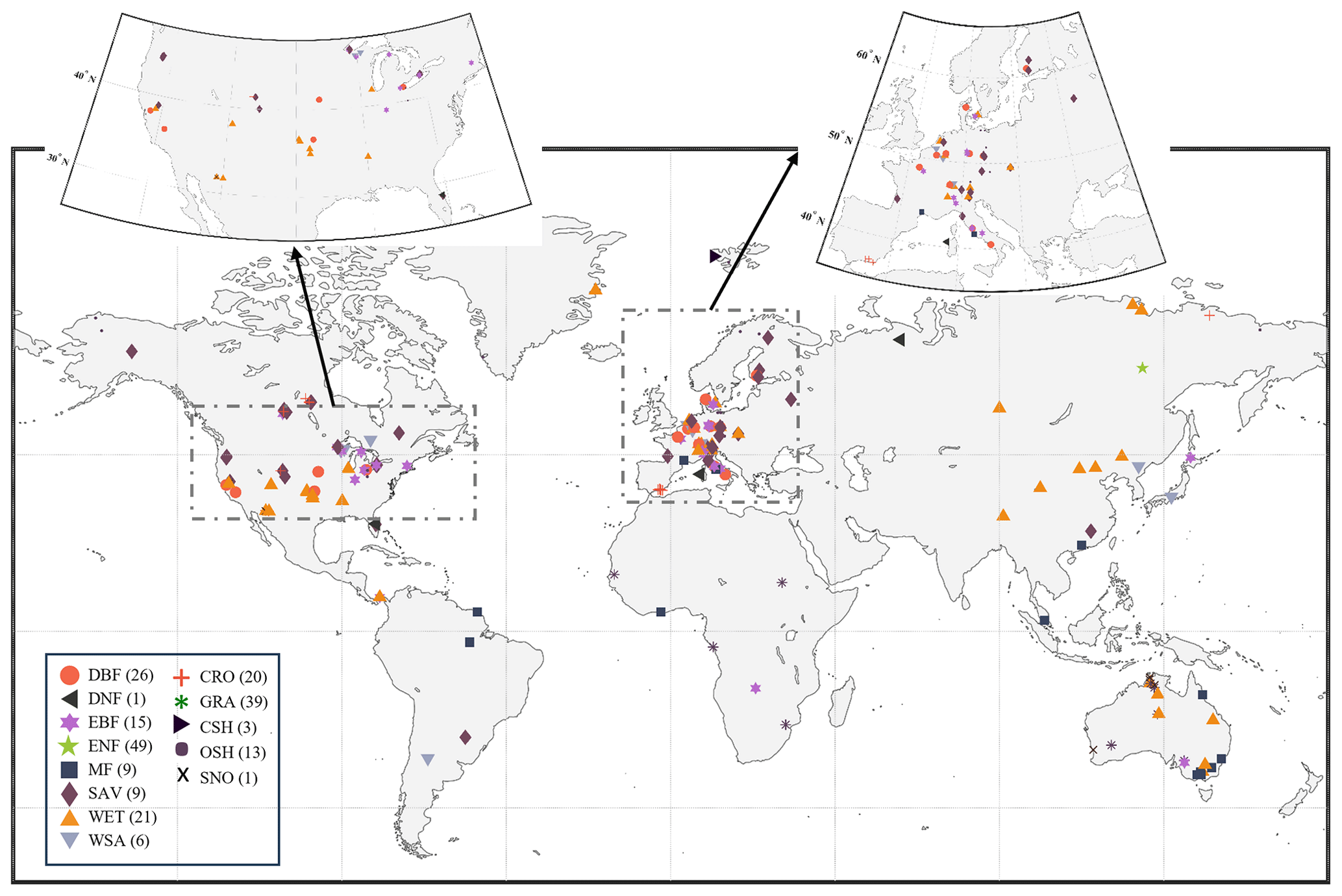
Figure 1Global distribution of selected FluxNet sites.
In this study, the fusion of products consisted of three steps: (1) the collocation method (IVD and EIVD) was used to calculate the random error variance of the selected input products, determine the regionally optimal products, and set an error threshold; (2) aiming for a minimum mean-square error (MSE), the weights of the different products on each grid were calculated; (3) the products were fused according to the weights to obtain a long sequence of evapotranspiration products. Since IVD and EIVD were developed by combining instrumental variable regression and the extended collocation system, a description of the TC and EC algorithms was also included.
3.1 Triple collocation analysis
Since its development in 1998, the implications and formulations of the triple collocation problem have been investigated in many studies. Here, we used difference notation for demonstration.
The commonly used error structure for triple collocation analysis (TCA) is
where are three spatially and temporally collocated datasets; Θ is the unknown true signal for the relative geographical variable; αi and βi are additive and multiplicative bias factors against the true signal, respectively; and εi is the additive zero-mean random error.
The above structure is also a typical IV regression. Thus, this provides another perspective to introduce more variables (> 3) (Dong and Crow, 2017; Su et al., 2014) and polynomial models (Yilmaz and Crow, 2013; De Lannoy et al., 2007) to the standard TC. We recommend that the readers refer to Su et al. (2014) for a more detailed discussion on using the IV framework.
The basic assumptions adopted in TC are as follows: (i) linearity between the true signal and datasets, (ii) signal and error stationarity, (iii) independence between the random error and true signal (error orthogonality), and (iv) independence between random errors (zero ECC). Although many studies have indicated that some of these assumptions are often violated in practice (Li et al., 2018, 2022; Jia et al., 2022), the formulation based on these assumptions is still the most robust implementation (Gruber et al., 2016b). A discussion of these assumptions will be provided in the Discussion section.
The datasets first need to be rescaled against an arbitrary reference (e.g., X). The others are scaled through a TC-based rescaling scheme:
The overbar denotes the mean value, and and are the scaling factors as
where is the average operator and σij is the covariance of datasets i and j.
Subsequently, the error variances could be estimated by averaging the cross-multiplied dataset differences as follows:
Expanding the bracket and expressing the rescaling factors yields
When selecting various scaling references, it is essential to note that the absolute error variances remain consistent. However, this choice can have an impact on the estimation of data sensitivity to the actual signal (), which serves as a crucial indicator for comparing spatial error patterns. In order to address the reliance on a specific scaling reference, Draper et al. (2013) introduced the fractional root-mean-squared error (fMSEi). This measure is obtained by normalizing the unscaled error variance with respect to the true signal variance:
where SNR is the normalized signal-to-noise ratio. SNR =0 indicates a noise-free observation, while SNR =1 corresponds to the variances of estimates equal to that of the true signal.
Following similar ideas, McColl et al. (2014) extended the framework to estimate the data–truth correlation, known as the ETC:
In comparison to the conventional coefficient of determination Rij, which is influenced by data noise and sensitivity, it is important to note that is merely based on the dataset i, whereas Rij is influenced by both the dataset i and reference j. In other words, incorporates the dependency on the chosen reference. Thus, TC-derived fMSEi and serve as superior indicators for assessing the actual quality of data, as discussed by Kim et al. (2021b) and Gruber et al. (2020).
3.2 Double instrumental variable technique
The assumed error structure in TC is also a typical instrumental variable (IV) regression. In practical usage, finding three completely independent sets of products is usually tricky. Su et al. (2014) effectively improve the applicability of the TC method by using the lag-1 time series (e.g., from one of the two sets of data as the third input for TC. In this way, we only need two independent products for input.
Such a process includes another assumption that all the datasets contain serially white errors (i.e., , zero auto-correlation). Building upon this, Dong et al. (2019) utilize the lag-1 time series from both datasets as inputs and propose the more stable IVD method.
For a double input , the linear error model and related lag-1 time series can be expressed as
where I and J are the lag-1 time series of X and Y, respectively.
Assuming product errors are mutually independent and orthogonal to the truth, the covariance between the products is expressed as
where is the auto-covariance. Therefore, the IVD-estimated dynamic range ratio scaling factors yield
Hence, the random error variances of X and Y can be solved as
3.3 Extended double instrumental variable technique
Furthermore, by adopting the designed matrix in the EC method (Gruber et al., 2016a), Dong et al. (2020a) present the EIVD method to estimate the error variance matrix with only two independent datasets.
For a triplet input , the dynamic range ratio scaling factors can be estimated as follows:
where is the auto-covariance of the inputs. Subsequently, the sensitivity and absolute error variance of the dataset follow
The cross-multiplied factors can be estimated by
Hence, for a triplet with an input of , the matrix notation of the above system with y=Ax is given as follows.
Likewise, the least-squared solution for the unknown x is then solved by
3.4 Weight estimation
Our objective is to predict an uncertain variable, such as ET over time at a specific location, by utilizing parent products that may contain random errors. The underlying concept of weighted averaging is to extract independent information from multiple data sources to enhance prediction accuracy by mitigating the effects of random errors. The effectiveness of this approach relies on the independence of the individual data sources under consideration. Weighted averaging has found applications in various fields following the influential work of Bates and Granger (1969), who proposed an optimal combination of forecasts based on a minimum MSE criterion. In this context, the term “optimal” refers to minimizing the variance of residual random errors in the least-squares sense. Mathematically, this weighted average can be expressed as follows:
where is the merged estimate; contains the temporally collocated estimates from N different parent products, which are merged with a relative zero-mean random error ; and contains the weights assigned to these estimates, where and ensure an unbiased prediction.
The averaging weights can be expressed as the solution to the problem:
where E is the operator for mathematical expectation. The solution of this problem is determined by the individual random error characteristics of the input datasets and can be derived from their covariance matrix (Bates and Granger, 1969; Gruber et al., 2017; Kim et al., 2021b):
where E(eeT) is the N×N error covariance matrix that holds the random error variance of the parent products in the diagonals and relative error covariances in the off-diagonals. is a ones vector of length N. represents the resulting random error variances of the merged estimate.
When only two groups of products are used as input (N=2), it is generally assumed that the errors between them are independent. In this case, the weights are as follows:
In most cases, we can identify three sets of products as inputs (N=3). In this scenario, we consider the possibility of error homogeneity, assuming a non-zero ECC exists between inputs 1 and 2. In this case, the error matrix can be represented as
The weights can then be written as
It is essential to acknowledge that, before applying these weights for merging the datasets, it is necessary to address any existing systematic differences. Typically, this is achieved by rescaling the datasets to a standardized data space. Consequently, the weights can be derived from the rescaled datasets using Eqs. (2)–(3) and converge accordingly. This procedure ensures the accuracy and reliability of the merged datasets for further analysis.
If ECC is not considered (i.e., setting ), Eq. (22) represents the weight calculation method commonly used in most TC fusion studies. In contrast to the fusion studies mentioned above for evapotranspiration products, for the first time, the consideration of non-zero ECC is incorporated into the fusion process and integrated into the weight calculation. Yilmaz and Crow (2014) demonstrated that TC underestimates error variances when the zero ECC assumption is violated. Li et al. (2022), in their evaluation study of global ET products using the collocation method, also indicated the existence of error homogeneity issues between commonly used ET products (such as ERA5L and GLEAM), necessitating the consideration of the influence of non-zero ECC. The merging technique employed in this study provides a more explicit characterization of product errors and facilitates the derivation of more reliable weight coefficients, thereby achieving promising fusion outcomes.
The differences in results are evaluated at the site scale by contrasting the scenarios without considering non-zero ECC and directly using simple averages to compare and validate the advantages of the weight calculation method used in our study.
3.5 Merging combination
In this study, we employ five commonly used global land surface ET products as described in the Datasets section. PMLv2 and FluxCom-RS have an original resolution of 0.083° and an 8 d average. In this research, they are interpolated to 0.1° resolution, and the values for each data period of 8 d are kept consistent. For example, the values for 5 March to 12 March 2000 are the same. ET values often exhibit variability over an 8 d period, making the use of an 8 d average to represent temporal dynamics potentially introduce further uncertainties. This operation is performed to ensure adequate data for the collocation analysis (Kim et al., 2021a). We openly acknowledge the possible sources of error and express our commitment to addressing and improving them in future work.
As mentioned in the Methods section, it is vital to consider the issue of random error homogeneity among different products before applying the collocation method. Although the EC or EIVD methods can be used to calculate the ECC between specific pairs of products, it is necessary to determine which pairs of products have non-zero ECC conditions. In previous research, Li et al. (2022) employed five collocation methods (IVS, IVD, TC, EIVD, and EC) to analyze the performance of five sets of ET products (ERA5L, PMLv2, FluxCom, GLDAS2, and GLEAMv3) at the global scale and applied the EC and EIVD methods to calculate the ECC between the different products. The results indicated a relatively significant error homogeneity between PMLv2 and FluxCom at a resolution of 0.1° (with a global average ECC of approximately 0.3). The error homogeneity could be attributed to both products utilizing GLDAS meteorological data as input, despite their different methods for ET estimation. At a resolution of 0.25°, ERA5L and GLEAM exhibited a more apparent error correlation (with a global average ECC of approximately 0.4). Considering the long temporal data of GLEAMv3 version a, ECMWF meteorological data were chosen as the driving force, making the error correlation between the two products predictable.
Therefore, this study assumes that non-zero ECC situations occur between PMLv2–FluxCom and ERA5L–GLEAM. We also calculated the possible ECC situations among other products, presented in the Discussion section and the Supplement. Based on the analysis, our assumed non-zero ECC situations align reasonably well with the actual circumstances.
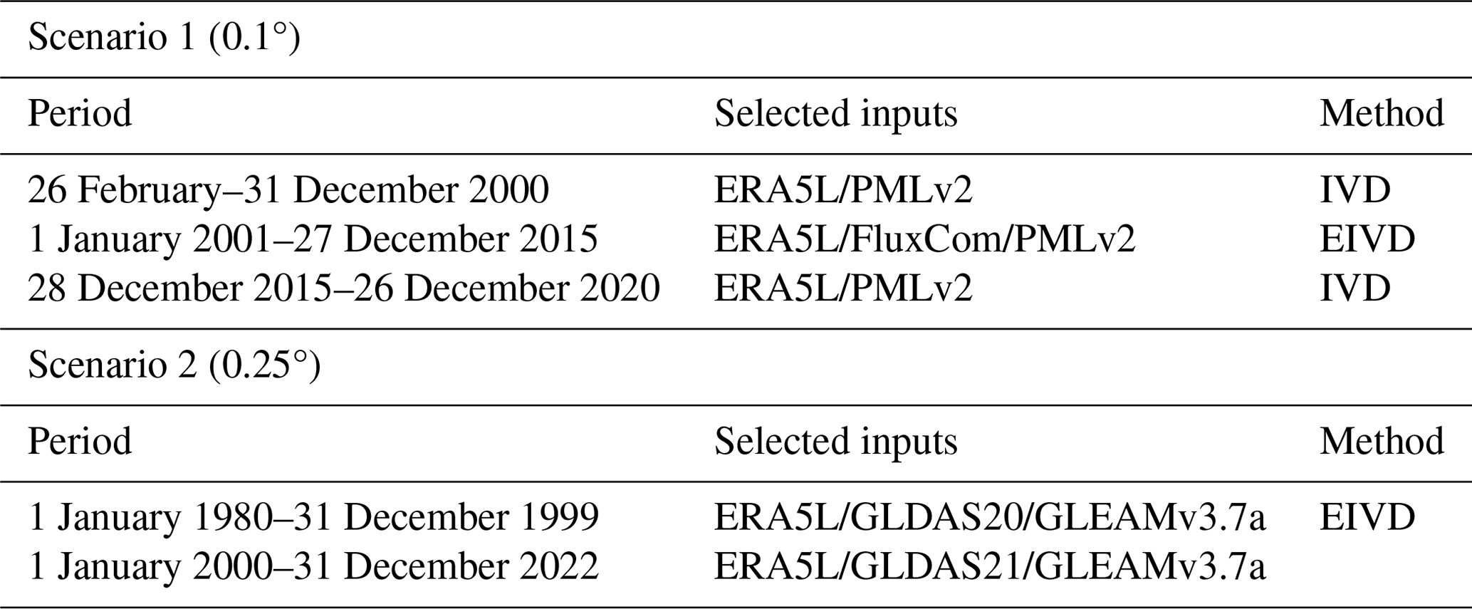
In addition, previous research suggests that the IVD method outperforms the IVS method in scenarios involving two sets of inputs, while the EIVD method is considered more reliable than the TC method in situations with three sets of inputs (Li et al., 2022; Kim et al., 2021a). Therefore, in this study, the IVD and EIVD methods are selected for computation based on different combinations of inputs. Table 2 presents the data and methods used during the corresponding periods. When only two sets of products are available, we employ the IVD method for fusion and calculate weights using Eq. (20). When three sets of products are available, we utilize the EIVD method for fusion and calculate weights using Eq. (22).
It should be noted that the same product can have different versions. In this study, appropriate versions are selected based on the following principles: (1) selecting based on the corresponding data coverage duration and ensuring more products to gain more information; (2) choosing the latest version while considering the assumption of non-zero ECC conditions; and (3) making efforts to select the exact product versions for different periods to avoid uncertainties caused by version changes. We selected a subset of sites to compare the fusion results using different versions, and the corresponding details will be presented in the Discussion section.
3.6 Evaluation indices
Five statistical indicators, i.e., root-mean-squared error (RMSE), Pearson's correlation coefficient (R), mean absolute error (MAE), unbiased RMSE (ubRMSE), and Kling–Gupta efficiency (KGE), are selected for comparison with existing products. The relative equations are shown as follows:
where sim is the simulations, and obs is the observation as a reference.
The modified KGE (Kling et al., 2012) offers insights into reproducing temporal dynamics and preserving the distribution of time series, which are increasingly used to calibrate and evaluate hydrological models (Knoben et al., 2019). For a better understanding of the KGE statistic and its advantages over the Nash–Sutcliffe efficiency (NSE), please refer to Gupta et al. (2009). The equation is given by
where σobs and σsim are the standard deviations of observations and simulations; μobs and μsim are the mean of observations and simulations. Similar to NSE, KGE = 1 indicates perfect agreement of simulations, while KGE<0 reveals that the average of the observations is better than the simulations (Towner et al., 2019).
In this study, we aimed to compare and evaluate the performance of fused products at both site and global scales. At the site scale, the performance of the fused products was evaluated against 212 FluxNet observations and compared with other products, including the simple average. At the global scale, the mean and temporal variations of the land surface ET calculated by the fused products were compared with those of other products.
4.1 Analysis of error variances and weights
This section examines the random error variances and identifies the predominant product based on assigned weights for the 0.1 and 0.25° inputs obtained through the EIVD method.
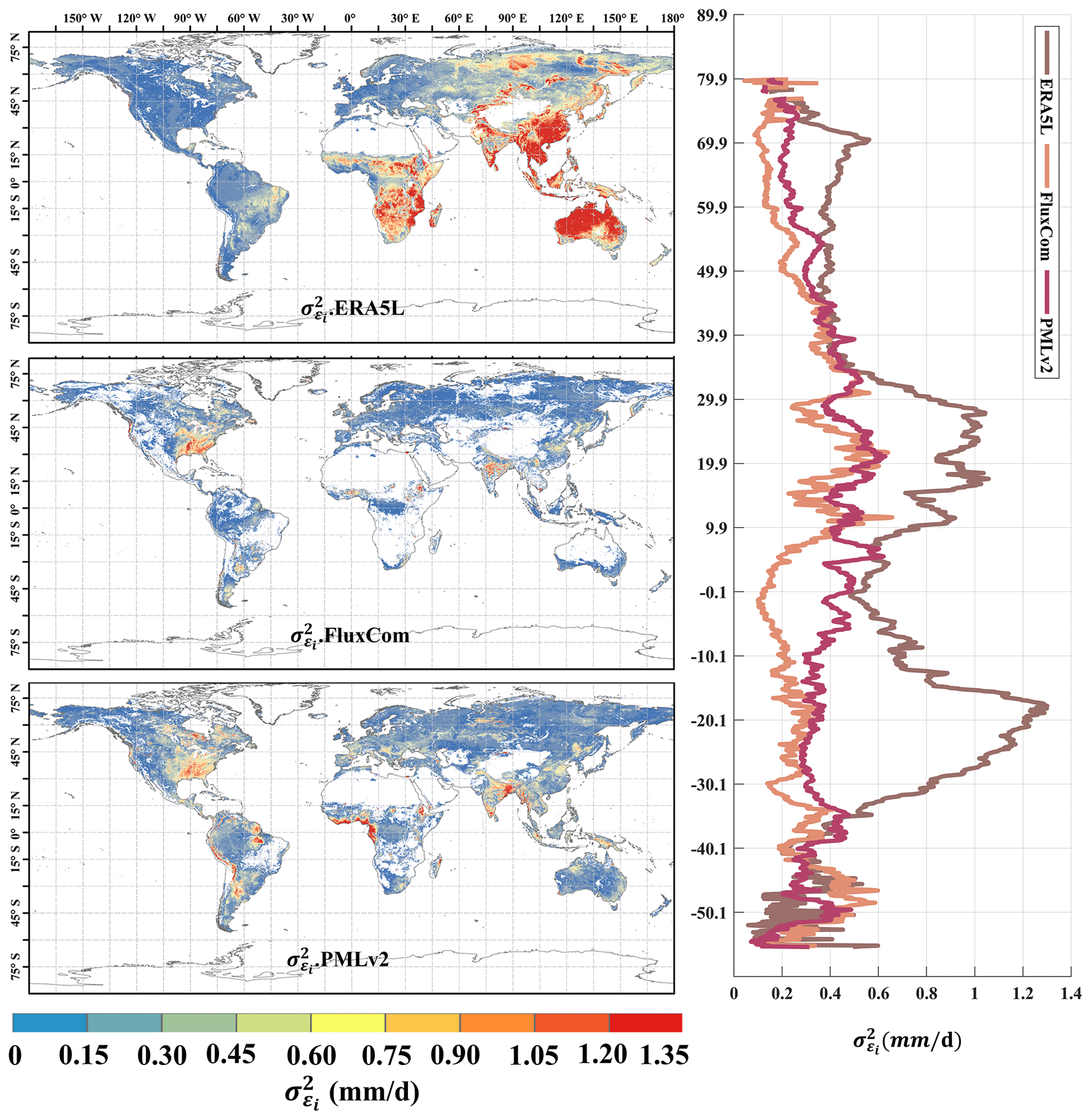
Figure 2Global distribution of absolute error variances () of ERA5L, FluxCom, and PMLv2 using EIVD at 0.1° from 2001 to 2015, depicted alongside the corresponding variation curves of the average with latitude.
Figure 2 represents the random errors of the correlation products calculated using the EIVD method from 2001 to 2015 at 0.1°, where a non-zero ECC is assumed between FluxCom and PMLv2. The areas with missing values are due to the absence of data from either FluxCom or PMLv2 in those regions. The global random error variances (mean ± standard deviation) obtained using the EIVD method are as follows: ERA5L: 0.58 ± 0.53 mm d−1, FluxCom: 0.12 ± 0.13 mm d−1, and PMLv2: 0.17 ± 0.14 mm d−1. These results indicate that FluxCom performs best overall, while ERA5L performs poorest. Regarding the spatial distribution, regions with more significant random errors in ERA5L are mainly located in East Asia, Australia, and southern Africa. On the other hand, FluxCom and PMLv2 show relatively more considerable uncertainties in the southeastern United States. The latitude distribution reveals that ERA5L has the highest uncertainty, primarily in the vicinity of 20 to 30° north and south, consistent with its spatial distribution.
It is important to note that, due to missing data in specific regions at 0.1°, such as northern Africa, the Sahara region, northwestern China, or Australia, the error results obtained may not accurately reflect the performance of FluxCom and PMLv2 in these areas. Considering the current results, we can cautiously conclude that FluxCom and PMLv2 demonstrate better performance. Future data supplementation in these regions would further enhance our ability to analyze the products' accuracy.
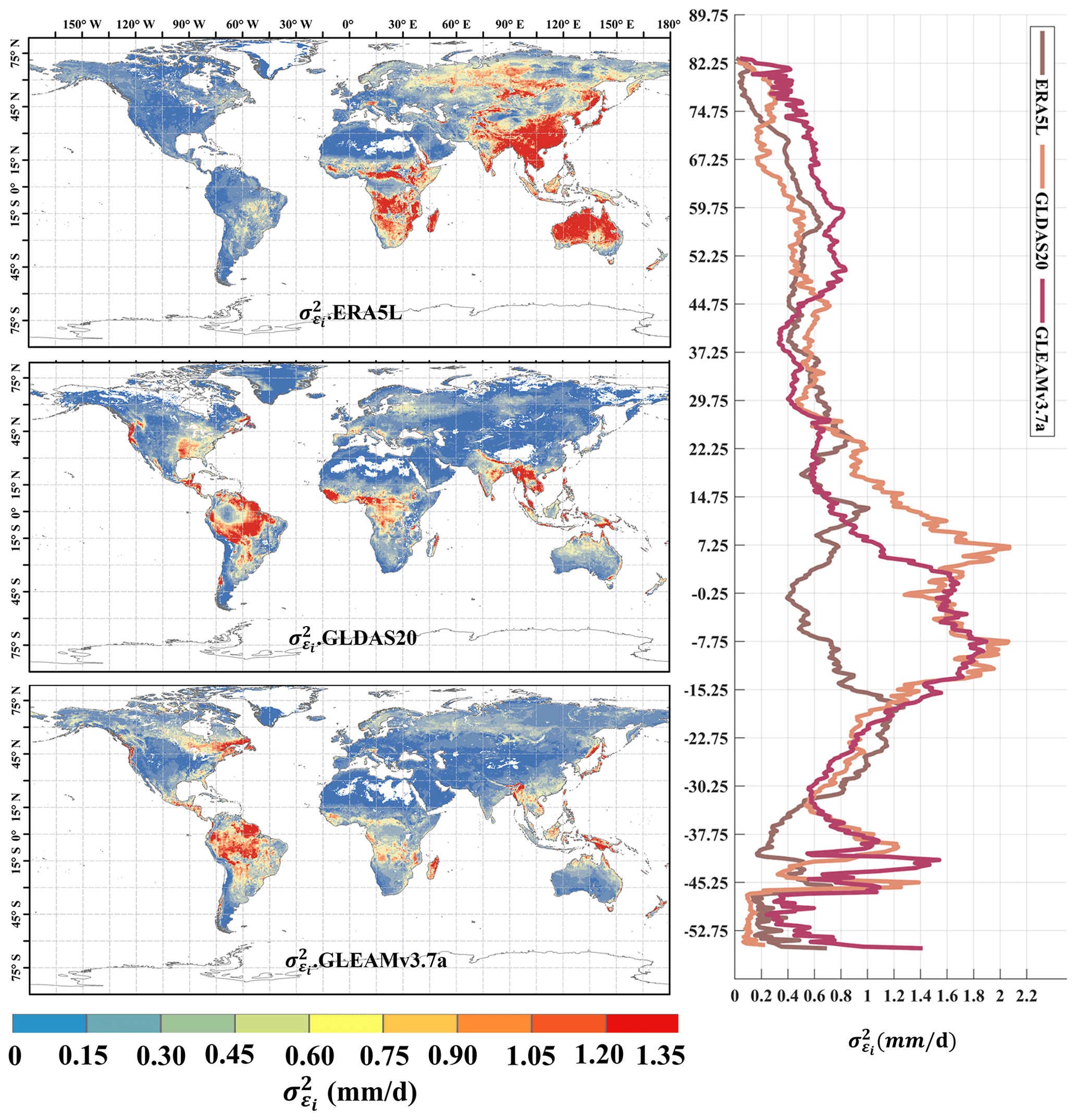
Figure 3Global distribution of absolute error variances () of ERA5L, GLDAS2.0, and GLEAMv3.7a using EIVD at 0.25° from 1980 to 1999, depicted alongside the corresponding variation curves of the average with latitude.
The distribution of random error variance for ERA5L (0.59 ± 0.58 mm d−1), GLDAS2.0 (0.37 ± 0.44 mm d−1), and GLEAMv3.7a (0.38 ± 0.36 mm d−1) from 1980 to 1999 at 0.25° is shown in Fig. 3. Here, we assumed a non-zero ECC between ERA5L and GLEAM. The ERA5L data were resampled from a 0.1° resolution to 0.25°, and their error distribution pattern is like that of the 0.1° resolution. It exhibits higher uncertainties in East Asia, Australia, and southern Africa. GLDAS and GLEAM exhibit relatively higher uncertainty over the southeastern United States and the Amazon Plain. GLDAS and GLEAM show similar performance among the three products, while ERA5L performs relatively worse. Regarding the average distribution with latitude, ERA5L demonstrates a more even distribution, whereas GLDAS and GLEAM exhibit relatively higher uncertainties in tropical regions.
The ET calculations in both GLDAS and GLEAM involve complex surface parameterization processes. In tropical regions, the high non-heterogeneity in land covers poses a challenge, and the 0.25° resolution grid may not capture the intricacies of the underlying surface conditions. This mismatch could impact the parameterization process, leading to errors. Future work could involve in-depth model analyses or sensitivity experiments to identify sources of error in complex ET models, facilitating improvements.
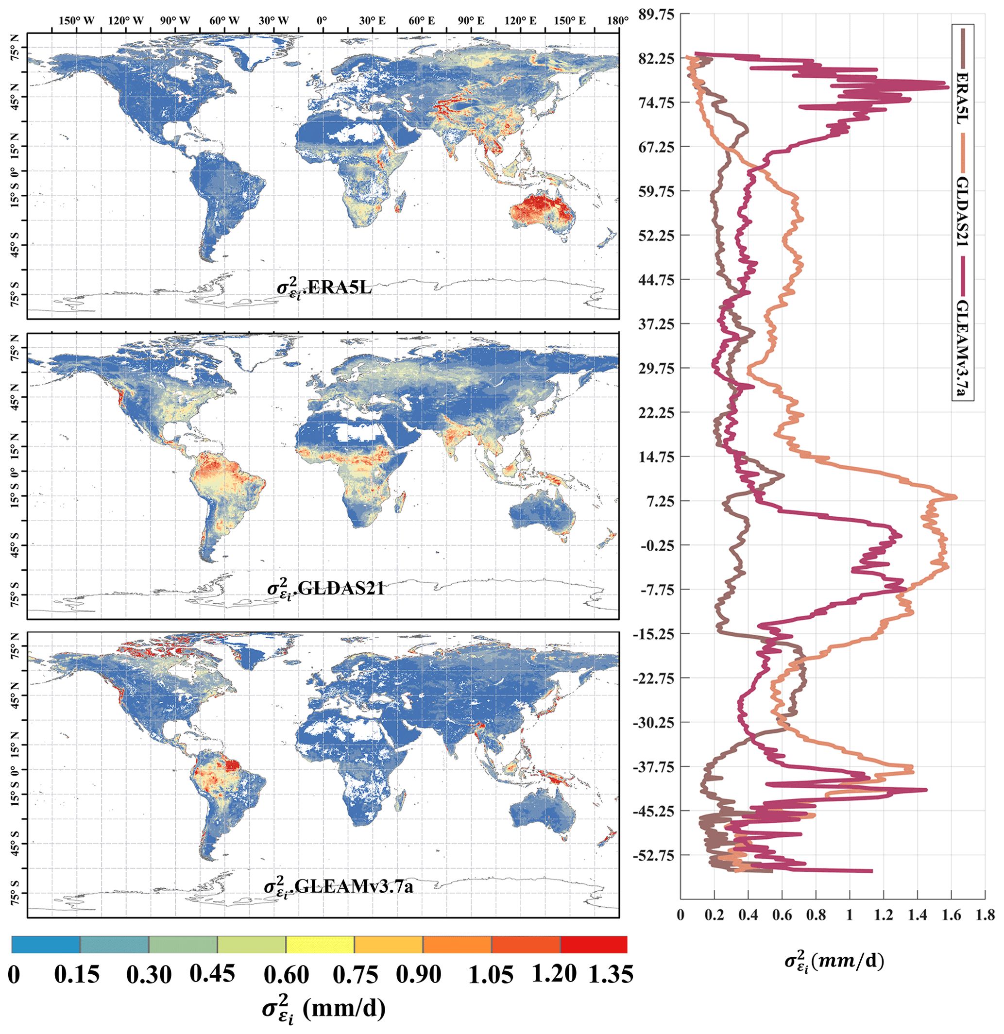
Figure 4Global distribution of absolute error variances () of ERA5L, GLDAS2.1, and GLEAMv3.7a using EIVD at 0.25° from 2000 to 2022, depicted alongside the corresponding variation curves of the average with latitude.
In addition, Fig. 4 presents the distribution of random error variance for ERA5L (0.32 ± 0.33 mm d−1), GLDAS2.1 (0.35 ± 0.29 mm d−1), and GLEAMv3.7a (0.38 ± 0.36 mm d−1) from 2000 to 2022 at a resolution of 0.25°. The non-zero ECC assumption was made between ERA5L and GLEAM. In this combination, ERA5L shows significantly lower errors than in previous periods, indicating an improved ERA5L performance during this time frame. However, ERA5L still exhibits more significant errors in the East Asian and Australian regions compared to the other two datasets. The overall errors for GLDAS and GLEAM have also decreased, but there are still random error variances exceeding 1.0 mm d−1 in the Amazon Plain and the Indonesian region. Regarding the latitudinal distribution, ERA5L shows relatively smooth changes, while GLDAS and GLEAM exhibit similar trends. However, GLEAM demonstrates a noticeable increase in errors near the Arctic.
Next, in Fig. 5, we present the dominant product for each grid cell in the three scenarios, where “dominance” refers to the product with the highest assigned weight. The results in Fig. 5 indicate that, at 0.1° resolution, the weights for FluxCom and PMLv2 are significantly higher than ERA5L, aligning with the error calculations presented in Fig. 2. This underscores the effectiveness of error and weight analysis based on collocation in reflecting product performance, thereby allowing for a rational adaptation of weights. At 0.25° resolution, the dominant regions for the ERA5L, GLDAS-2, and GLEAM products are relatively balanced. In the fusion scenario from 1980 to 1999, GLDAS20 predominantly covers the Northern Hemisphere, while GLEAM dominates the Southern Hemisphere, with ERA5L prevalent in the Amazon region. However, in the fusion scenario from 2000 to 2022, GLEAM's dominant region significantly expanded, primarily covering the central United States and southeastern China. The Amazon region continues to be dominated by ERA5L. The variation in the dominant products highlights that the calculation of product weights evolves with changes in the fusion scenario. The error and weight computation methods based on collocation can only provide the minimum MSE solution for a given combination of inputs. It is important to note that changes in inputs will impact the results.
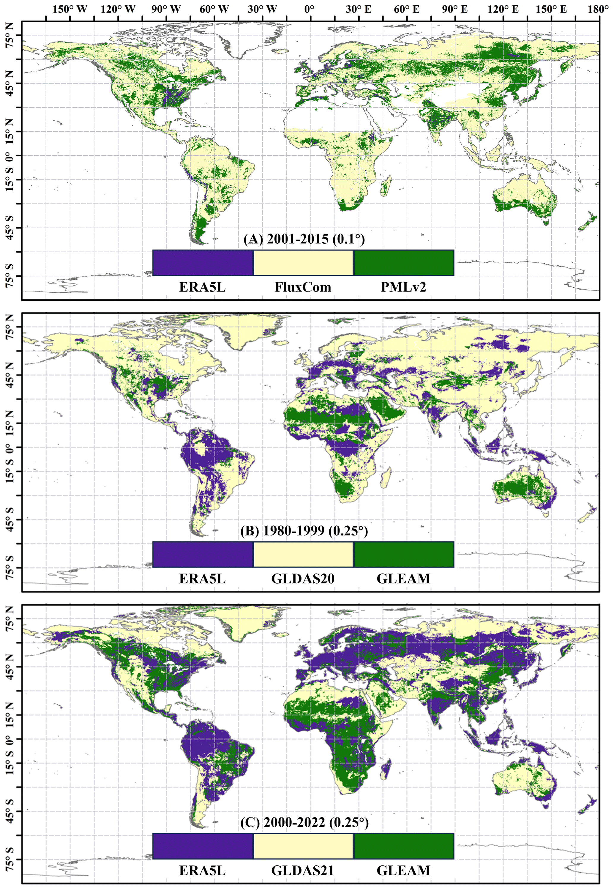
Figure 5Map of the prevailing product at individual pixels based on scenario-specific weights.
For the analysis at a resolution of 0.1°, we also applied the IVD method to calculate the errors between ERA5L and PMLv2 for two time periods: 2000 and 2015–2020. Since the analysis of product errors is not the focus of this paper, we provide the results of the IVD in the Supplement. Grids with higher random error variances correspond to smaller weights when calculating the weights. The weight distribution calculated at different time intervals is available in the Supplement.
4.2 Site-scale evaluation and comparison
At the site scale, the performance of CAMELE was compared with FluxNet as a reference. In this subsection, Fig. 6 and Table 3 correspond to each other, as they integrate data from 212 sites for all available periods, allowing for a comparative analysis of the performance of different products at different times. Similarly, Fig. 7 and Table 4 correspond to each other, where different product metrics were calculated for each site and the calculated metric results were subjected to statistical analysis.
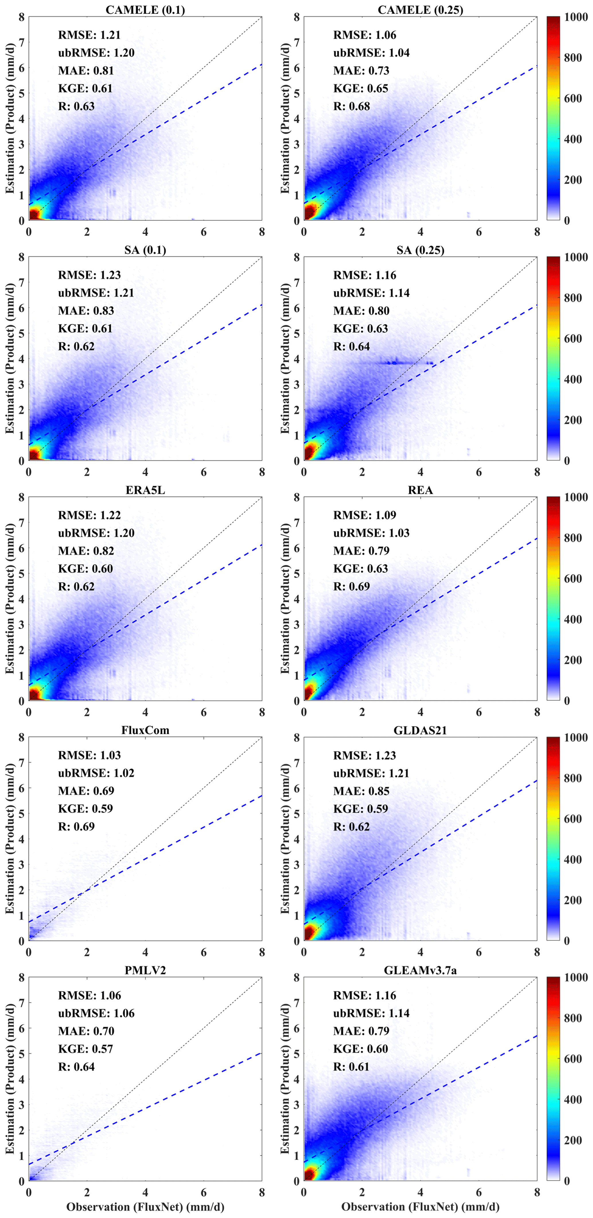
Figure 6Scatter plots of the product corresponding to the available period data from 212 FluxNet sites. The color bar represents the density, with darker colors indicating higher concentrations. The left and right columns present results for the 0.1 and 0.25° resolutions, respectively, with “SA” indicating the results for the simple average. Relevant statistical metrics are annotated in their respective figures.
The scatter plots in Fig. 6 demonstrate that CAMELE consistently performs at 0.1 and 0.25° resolutions. At 0.1° resolution, FluxCom and PMLv2 showed superior performance with fewer data points due to their original 8 d average resolution. CAMELE exhibited a performance like ERA5L. At 0.25° resolution, CAMELE performed comparably to the other datasets, demonstrating reasonable accuracy. Notably, there was an improvement in the KGE and R indices. The fitted line closely approximated the 1:1 line, indicating a solid agreement with the observed values. Moreover, the results obtained from the simple average were also acceptable, but SA (0.25°) had a concentration of data points between 2 and 4 mm d−1, possibly due to the inputs having a high concentration within that range. The assumption that a simple average implies equal performance of each product on every grid cell is inaccurate; variations in performance exist among different products across distinct grid cells (regions).
Table 3Average values of the different metrics for CAMELE and other fusion schemes corresponding to the available period data from 212 FluxNet sites. The bold sections indicate the schemes with the best performance in their respective metrics.
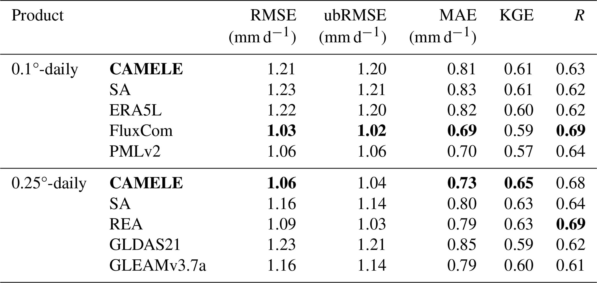
The information in Table 3 corresponds to Fig. 6 and presents the results of various product indicators. The bold parts indicate the products with the best corresponding indicators. The results indicate that CAMELE performed well at both the 0.1 and 0.25° resolutions, mainly showing improvements in the KGE and R indicators. FluxCom exhibited the best performance; however, considering that this product utilized FluxNet sites for result calibration, this phenomenon is reasonable. In this study, we pooled the data from all 212 available periods at the stations as a reference without considering the differences between individual sites. This approach provided an initial validation of the reliability of CAMELE at all the sites.
The information in Fig. 7 corresponds to the data presented in Table 4, which involve the calculation of five indicators at each site, followed by statistical analysis of these indicators. From the distribution of the violin plots, it can be observed that a violin plot with a closer belly to 1 indicates better results in terms of the R and KGE indicators. CAMELE performs well overall, closely resembling PMLv2 and FluxCom. On the other hand, the results obtained from the SA are relatively poorer. Regarding the RMSE, ubRMSE, and MAE indicators, a violin plot with a closer belly to 0 suggests fewer errors. CAMELE demonstrates a notable enhancement in performance at the 0.1° level. This suggests that the fusion method effectively reduces errors, aligning with the original intention of weight calculation, and it compares favorably with the products used in the merging scheme.
Additionally, FluxCom and PMLv2 exhibit minimal errors, which is expected considering their utilization of FluxNet sites for error correction. Furthermore, SA shows significantly larger errors. Although the SA method can compensate for positive and negative errors between inputs in some instances, it can also lead to error accumulation, as evidenced by the results in the violin plots.
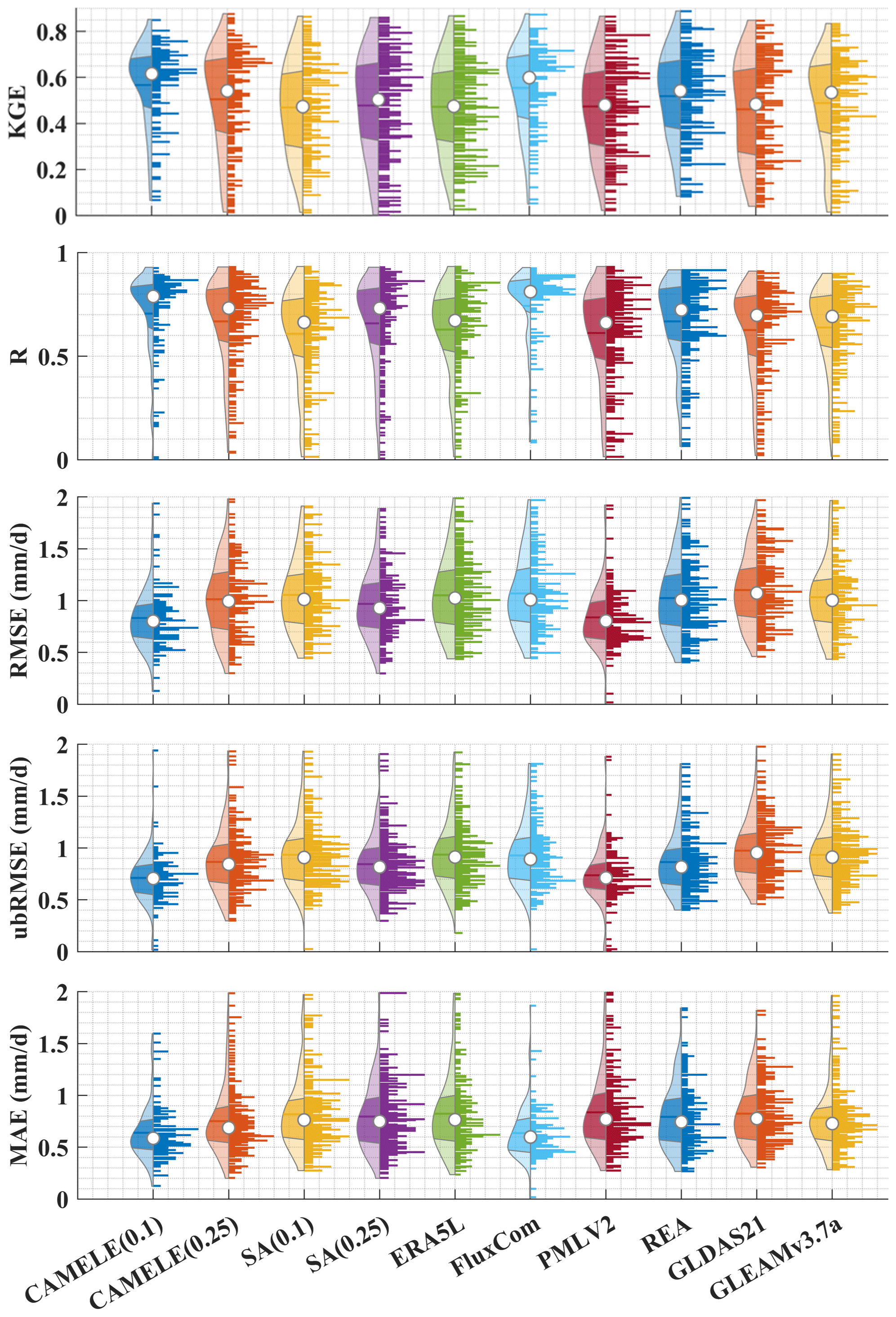
Figure 7Violin plots obtained by aggregating five different statistical indicators calculated separately for each site. In each violin plot, the left side represents the distribution, with the shaded area indicating the box plot, the dot representing the mean, and the right side showing the histogram.
Table 4Average values of indicators corresponding to different products, calculated based on the comprehensive results obtained for each site. The bold sections indicate the schemes with the best performance in their respective metrics.
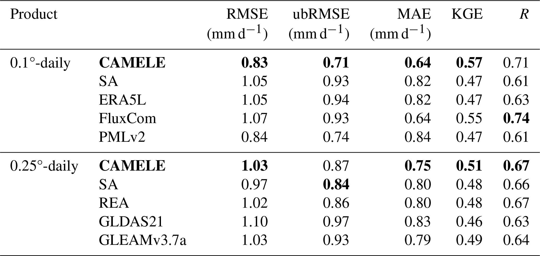
Table 4 presents the average values of different metrics in Fig. 7, boldly highlighting the optimal products corresponding to each metric. It can be observed that CAMELE exhibits significant improvements in performance at a resolution of 0.1°, particularly in terms of the error metrics RMSE and ubRMSE, surpassing other products. This further confirms the effectiveness of our fusion scheme in reducing product errors. Additionally, although the performance of CAMELE at a resolution of 0.25° is comparable to other products, there is still a slight decline compared to its performance at 0.1°. This can be attributed partly to the inherent errors in the input products and partly to the decreasing representativeness of FluxNet, which serves as the reference at the 0.25° grid. Nevertheless, we can still consider CAMELE to have good accuracy.
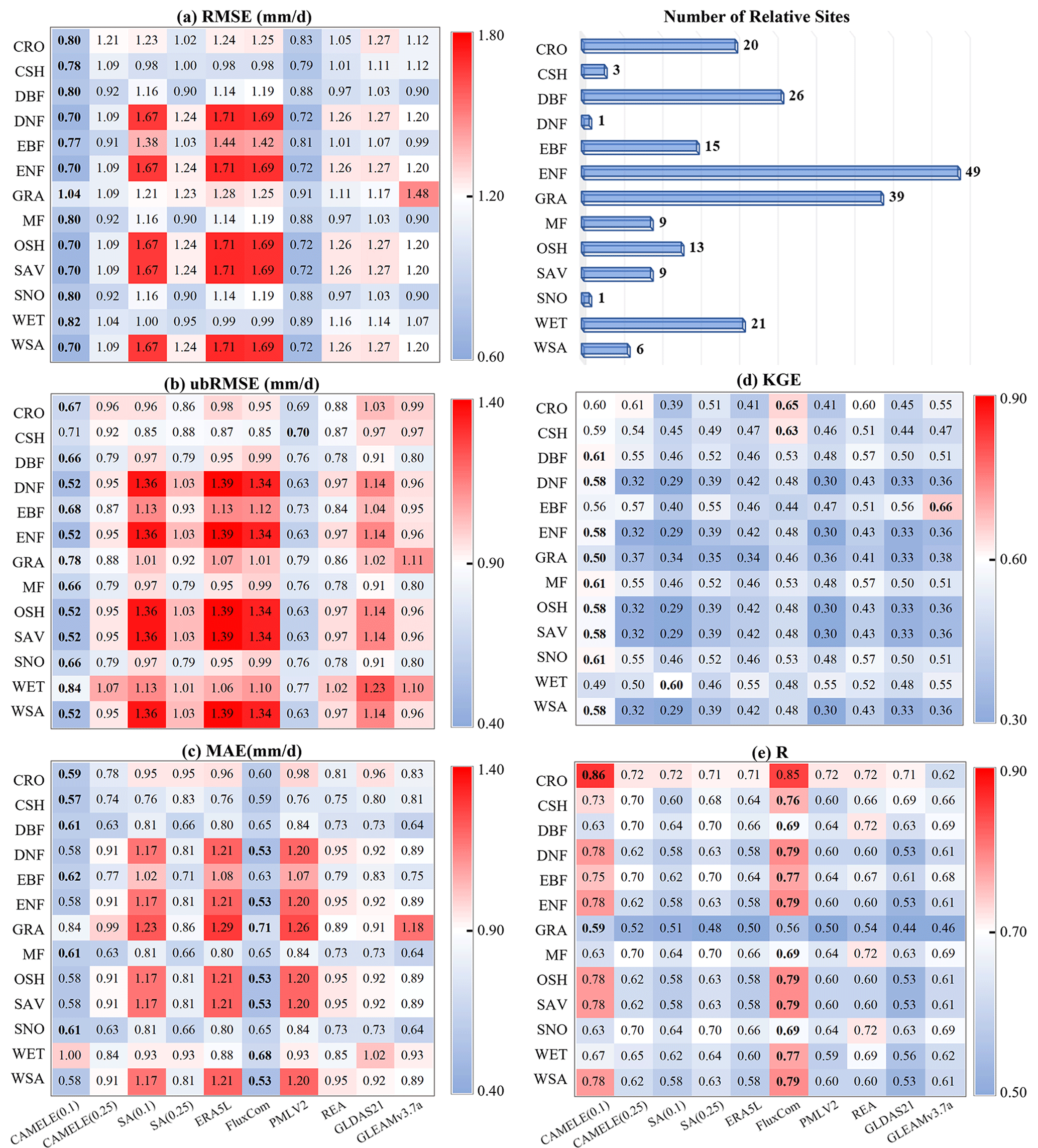
Figure 8Heatmaps of five statistical indicators, where each row corresponds to the mean value for all sites of the specific PFT, and each column corresponds to a product. The product with the best performance for that PFT is highlighted in bold within each row. Panels (a)–(c) represent three error indicators: RMSE, ubRMSE, and MAE. Panels (d)–(e) represent two goodness-of-fit indicators: KGE and R.
Table 5Optimal product corresponding to different PFTs under various statistical indicators against observations from FluxNet sites.
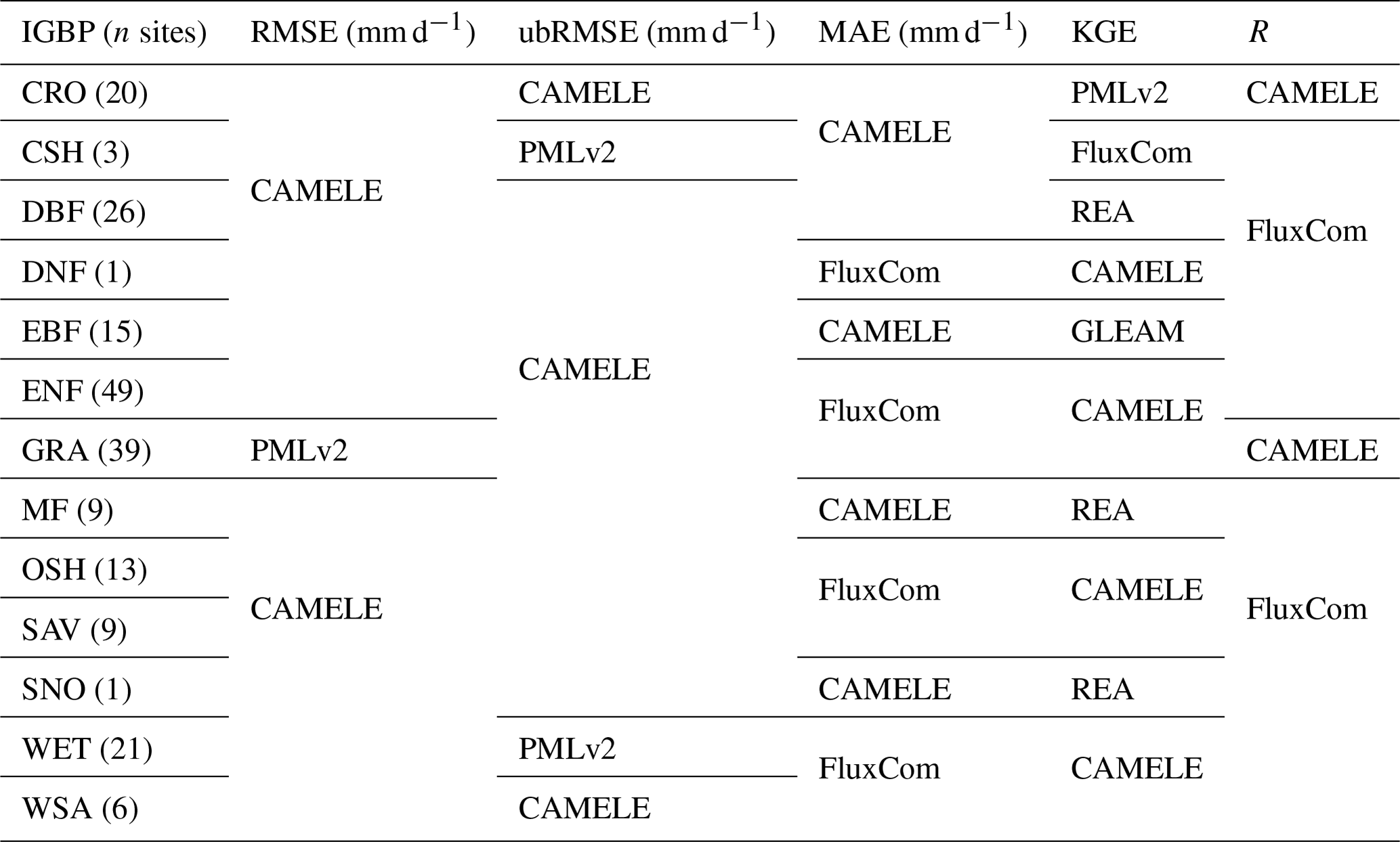
Furthermore, we classified 212 sites according to PFTs and analyzed the statistical indicators of different PFTs corresponding to each site. The results are represented in Fig. 8 as a heatmap, and the corresponding optimal products for other PFT sites are shown in Table 5. The results show that CAMELE performs the best in almost all the PFT categories, as indicated by various indicators, while on sites where other products perform better, CAMELE's indicators are comparable to the optimal products, albeit slightly inferior. This indicates that our fusion approach effectively combines the advantages of different products, resulting in superior fusion results across different vegetation types.
From the results, it is evident that CAMELE performs well across various vegetation types. To delve deeper into the reasons behind this performance, we conduct site-scale analyses at two resolutions, evaluating errors and computed weights for different PFT sites. These are visualized in radar chart format in Fig. 9.
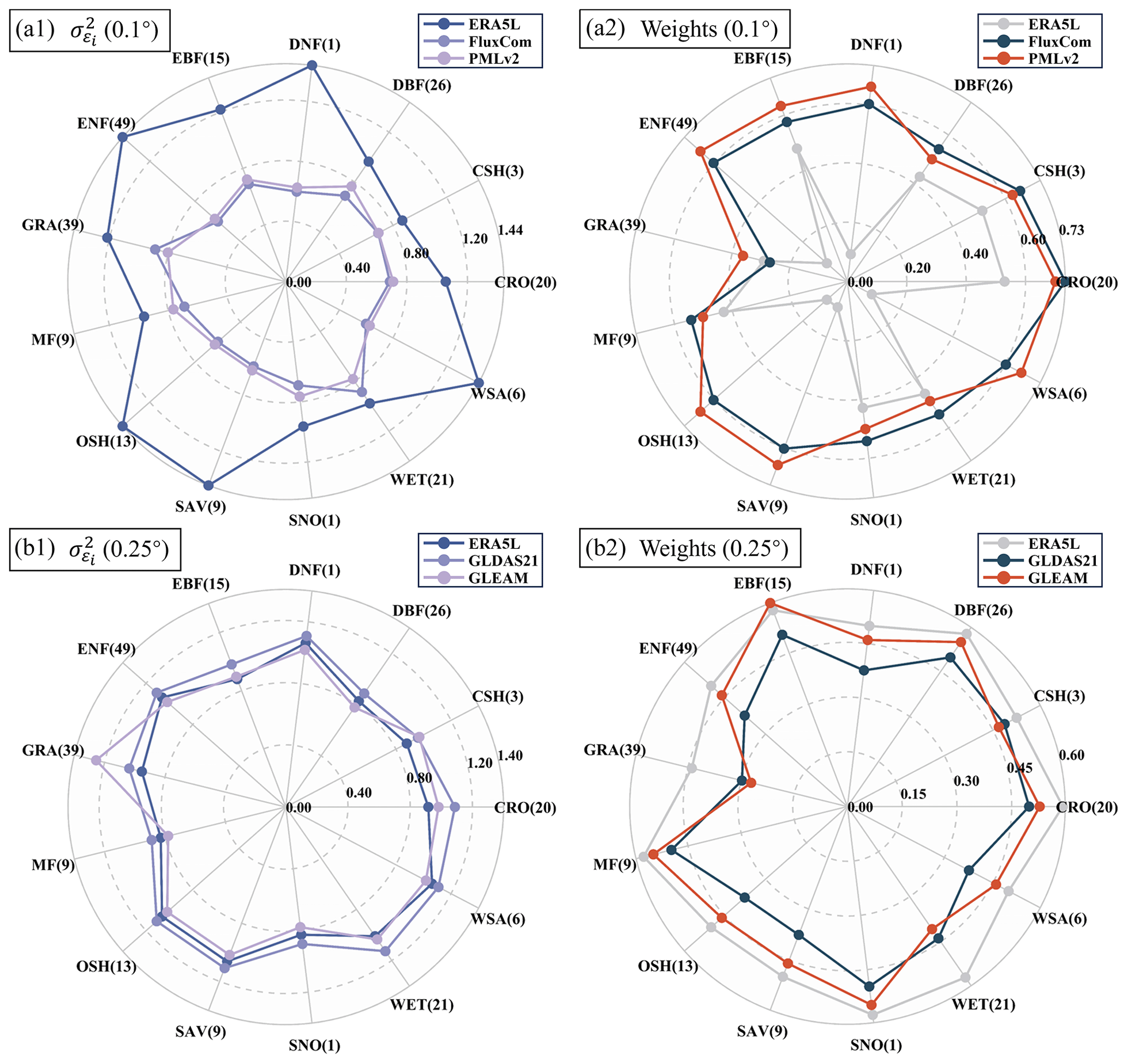
Figure 9Mean collocation-based errors and weights of different products at various PFT sites at (a) 0.1° and (b) 0.25° resolutions. The parentheses next to each PFT name denote the corresponding number of sites.
The results from Fig. 9 demonstrate that the error-weighting calculation method based on collocation effectively considers the error situation of inputs, thereby providing reasonable weight assignments. At 0.1° resolution, ERA5L's error is significantly higher across all the PFTs than FluxCom and PMLv2, resulting in relatively lower corresponding weights. FluxCom and PMLv2 exhibit closer performance, with higher weights at most of the PFT sites. At 0.25° resolution, ERA5L, GLDAS21, and GLEAM perform more evenly with minimal differences, resulting in closer weights. The weights for different inputs vary noticeably with changes in PFTs, depending on the performance of other products within the same combination. Products with more significant errors correspondingly have lower weights, affirming the rationale behind the fusion method. However, it is essential to note that the presented results depict the mean values of errors and weights across all the sites; there might be variations among sites with the same PFTs.
In summary, using the filtered daily-scale data from 212 FluxNet sites as a reference, we conducted a benchmark analysis with CAMELE and demonstrated its good fit with the observed data. Additionally, by comparing the performance of different products at each site, we further illustrated that CAMELE exhibits similar or slightly improved accuracy and minor errors compared to existing products.
4.3 Assessment and comparison of the multiyear average
In this section, we will first analyze and compare the performance of CAMELE with other products in estimating the multiyear mean and extreme values of ET at the site scale. Subsequently, a global-scale analysis will be conducted for the same periods (0.1°: 2001 to 2015; 0.25°: 2000 to 2017) to examine the distribution of the multiyear daily average ET calculated by different products. For site comparisons, we have selected monthly mean ET values and three quantiles (5th, 50th, and 95th) to represent the products' performance in estimating ET average and extreme values.
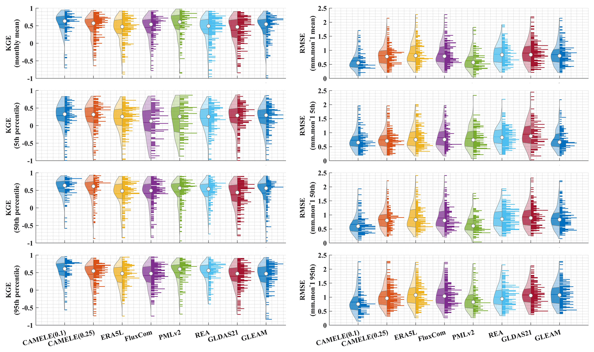
Figure 10Violin plots depicting the KGE and RMSE metrics calculated for CAMELE and other products based on the monthly mean, 5th, 50th, and 95th percentiles at each FluxNet site. The four left columns represent KGE plots, while the four right columns represent RMSE plots. The dots in the violin plots represent the median, and the horizontal lines represent the mean.
Table 6Average values of KGE and RMSE corresponding to different products, calculated based on the results obtained for each site. The bold sections indicate the schemes with the best performance in their respective metrics.
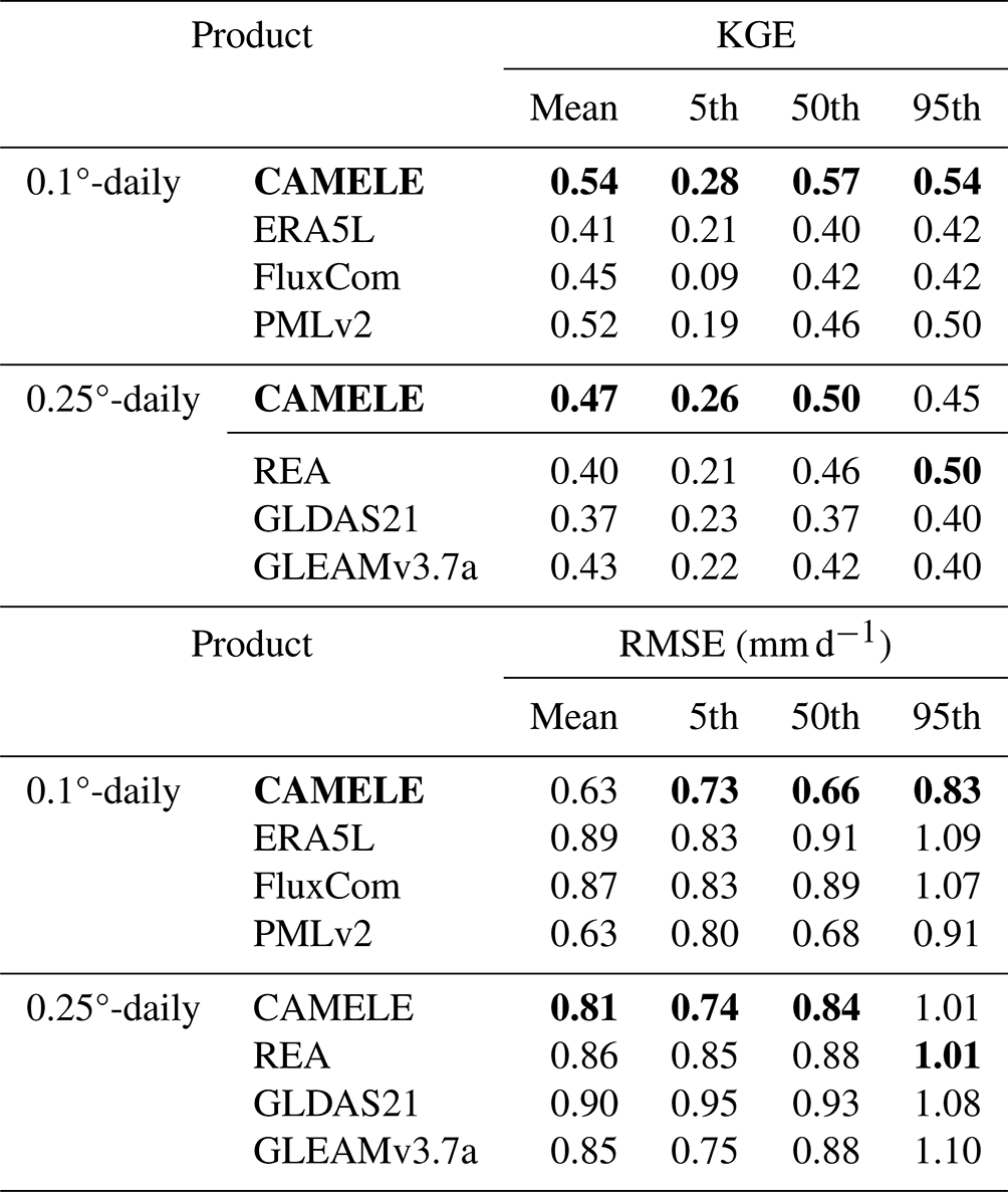
The information in Fig. 10 corresponds to the data presented in Table 6, which involve the calculation of the KGE and RMSE at each site, followed by statistical analysis. From the distribution of the violin plots, it can be observed that a violin plot with a closer belly to 1 indicates better results in terms of the KGE.
The results show that CAMELE outperforms other products in the estimation of monthly averages and the 5th, 50th, and 95th percentiles at both 0.1 and 0.25° resolutions. Its performance in capturing monthly averages is noteworthy, with a noticeable improvement in the KGE and RMSE metrics relative to the inputs. Examining the results for percentiles, CAMELE shows a relatively poorer estimation for shallow values (5th percentile) but still demonstrates some improvement compared to the input data, albeit influenced by input errors.
At 0.1°, PMLv2 and FluxCom perform just below the fusion result, aligning with the previous error and weight analysis. At 0.25°, GLEAM and REA closely follow CAMELE, with REA exhibiting slightly better estimation results for extremely high values (95th percentile) than CAMELE. Despite this, the analysis results still indicate that the products obtained reflect well the multiyear averages and extremes of ET, holding promise as reliable products for analyzing ET variations.
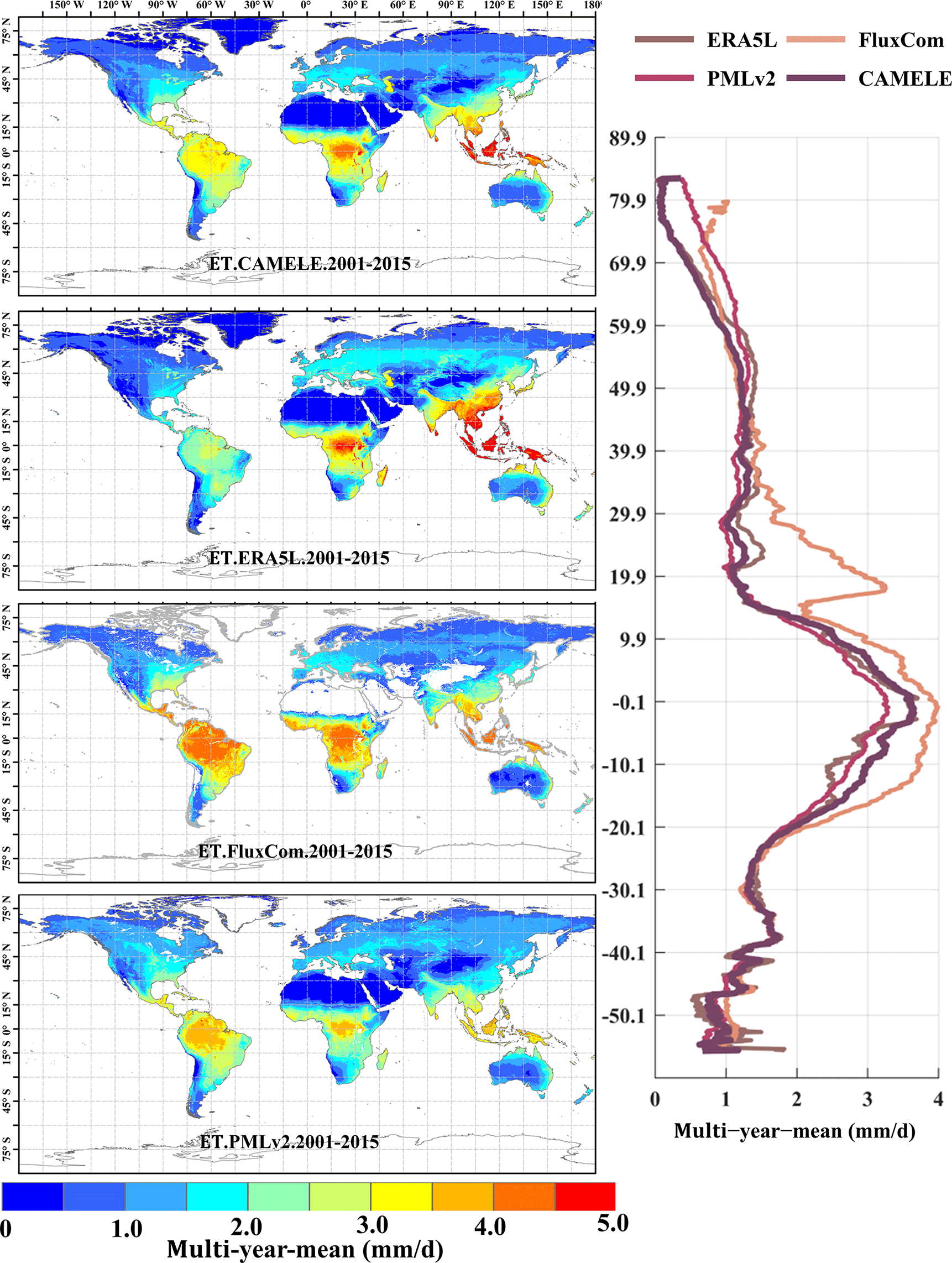
Figure 11Global distribution of multiyear daily average ET at 0.1° for CAMELE, ERA5L, FluxCom, and PMLv2, depicted alongside the corresponding variation curves of the multiyear daily average ET with latitude.
The results in Fig. 11 indicate significant differences in the multiyear daily average distribution of global ET among different products. Specifically, ERA5L shows noticeably higher values in East Asia than other products, while FluxCom and PMLv2 exhibit higher values in the Amazon rainforest and southern Africa regions. This distribution pattern is consistent with the error results obtained from the EIVD calculation, indicating that these products possess certain uncertainties in the regions. In terms of the latitudinal distribution pattern, except for FluxCom, which displays distinct fluctuations, the variability among the other products is relatively similar. This suggests that, despite spatial differences among the different products, they maintain consistency in the overall quantity.
Figure 12 presents the results with a resolution of 0.25°. It can be observed that, compared to the 0.1° distribution, the spatial distribution of annual average ET is more consistent among different products at 0.25°, showing larger ET values in tropical regions. The main differences are concentrated in the Amazon rainforest and the Congo Basin, where GLEAM and GLDAS results are higher than REA's. The assigned weights for REA's inputs (MERRA2, GLDAS, and GLEAM) are approximately equal in these two regions, each contributing about one-third to the overall calculation (Lu et al., 2021). This balanced allocation results in the REA being distributed among them roughly equally over multiple years in these two regions. The latitude variation plots show that the results from each product are very close, providing additional evidence for the reliability of CAMELE.
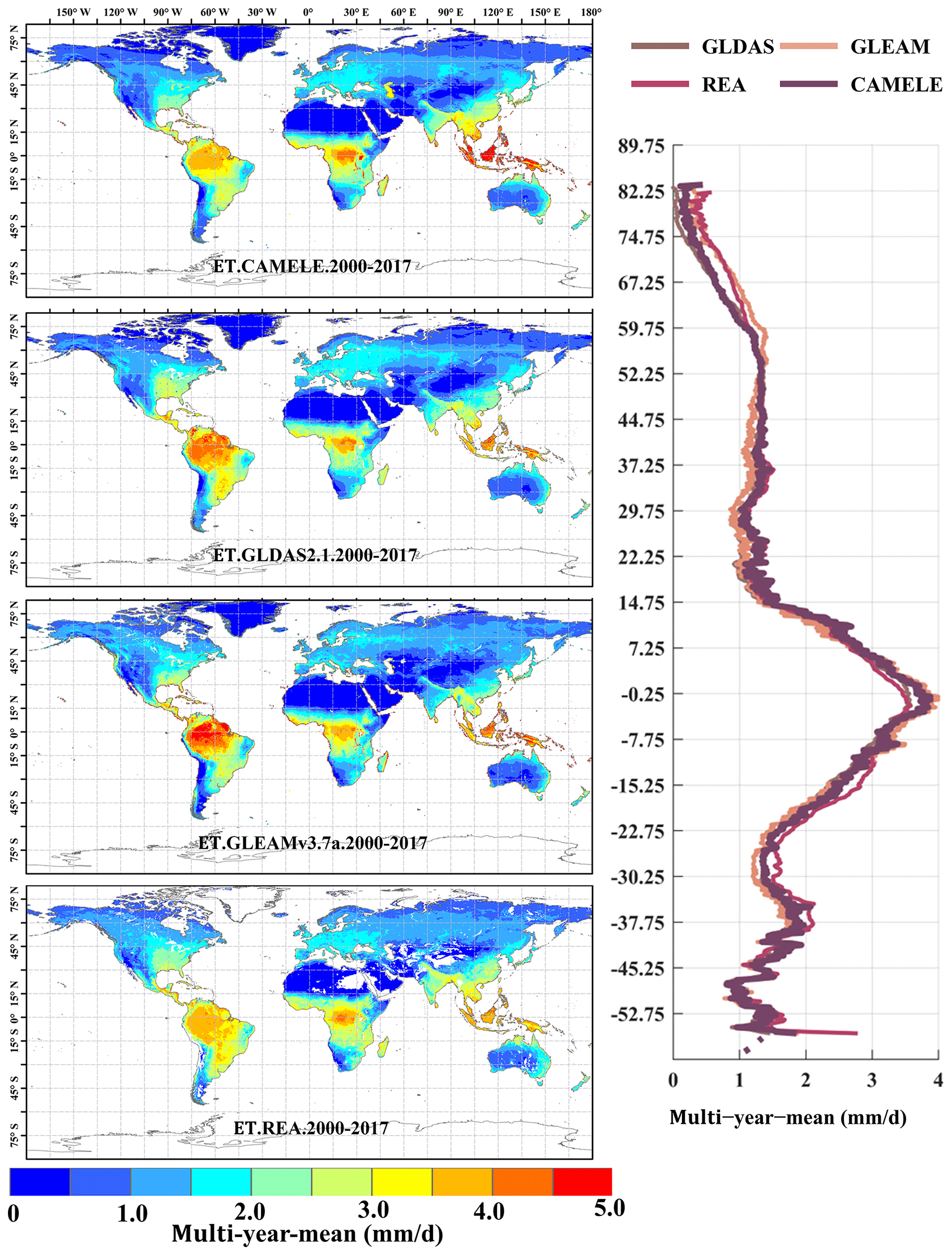
Figure 12Global distribution of the multiyear daily average ET at 0.25° for CAMELE, GLDAS2.1, GLEAMv3.7a, and REA, depicted alongside the corresponding variation curves of the multiyear daily average ET with latitude.
In parallel, it is worth noting that, despite the regional disparities that may arise when contrasting the trends by CAMELE with inputs, a noteworthy consistency emerges when examining these trends along latitudinal gradients. This notable alignment signifies the robustness of CAMELE to some extent. It underscores the capacity of CAMELE to capture ET patterns, providing further insights for the scientific community.
4.4 Assessment and comparison of linear trend and seasonality
In this section, we first validate and compare the performance of CAMELE with other products in estimating multiyear trends and seasonality at the site scale. Due to the inconsistent time lengths of FluxNet sites, trends at many sites are not significant. Therefore, we deliberately selected 13 sites with continuous ET observations for the same 11-year period (2004 to 2014) and with significant trends. The annual ET values for each year were calculated as the mean of the 13 sites for that year, allowing the computation of linear trends and seasonality. We employed singular spectrum analysis (SSA), which assumes an additive decomposition A = LT + ST + R. In this decomposition, LT represents the long-term trend in the data, ST is the seasonal or oscillatory trend (or trends), and R is the remainder.
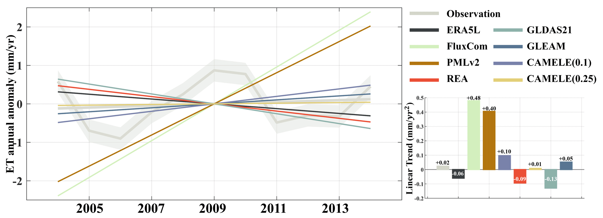
Figure 13Comparison of the linear trend from 2004 to 2014 among 13 FluxNet sites using CAMELE and other products. The trends have been subjected to SSA decomposition, removing seasonality. The gray enveloping line represents the mean plus the standard deviation of the 13 sites.
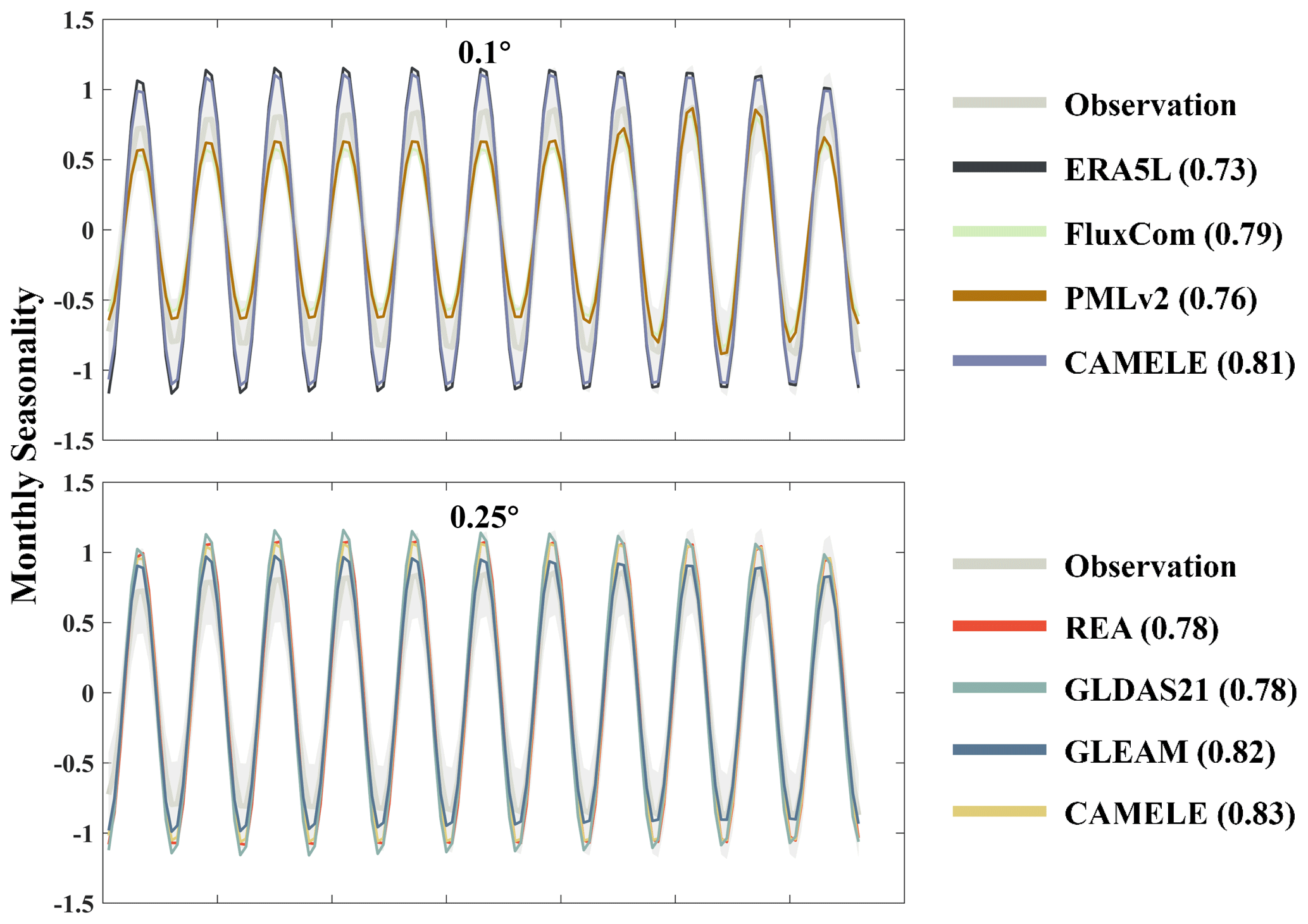
Figure 14Comparison of seasonal variations from 2004 to 2014 among 13 FluxNet sites using CAMELE and other products. The seasonality has been obtained through SSA decomposition, with the gray area representing the observed values. The parentheses in each product name indicate the KGE coefficient compared with the observed values.
In Figs. 13 and 14, based on observations from FluxNet sites, we analyzed the performance of CAMELE and other products in estimating the linear trend and seasonality of ET over multiple years. It is important to note that we only present the analysis results for 13 sites with continuous 11-year observations, and the performance of different ET products in trend estimation at individual sites still varies, not fully reflecting the overall performance on all grids in terms of trend and seasonality. Nevertheless, such a comparison can still provide valuable insights.
Examining the results of the linear trend, both PMLv2 and FluxCom exhibit a significant upward trend, well above the observations. By contrast, ERA5L, GLDAS, and REA show a noticeable downward trend, while CAMELE demonstrates a gradual upward trend closer to the observations. Additionally, GLEAM slightly outperforms CAMELE at a resolution of 0.25°. Overall, CAMELE shows good agreement with site observations in capturing the multiyear linear trend of ET.
Continuing with the analysis of seasonality, the KGE index comparing each product's results with observed values is provided in parentheses next to the product name. Generally, all the products exhibit a good representation of ET's seasonal variations. CAMELE's 0.1° seasonal results closely match FluxCom (with the two lines almost overlapping). However, the fluctuations it reflects are higher than the observed values.
This is likely due to keeping the 8 d average results of FluxCom consistent with PMLv2 every 8 d, and the variability in ET primarily originates from ERA5L results. This aspect may need improvement in subsequent research. At 0.25°, CAMELE's seasonal representation is closer to the observed results. The differences in CAMELE's performance at the two resolutions are mainly attributed to input variations, which we discuss in the following section as potential areas for improvement.
Table 7Comparison of CAMELE results at 13 continuous 10-year observational sites. (a) Comparison of linear trends. (b) KGE values for monthly seasonality.
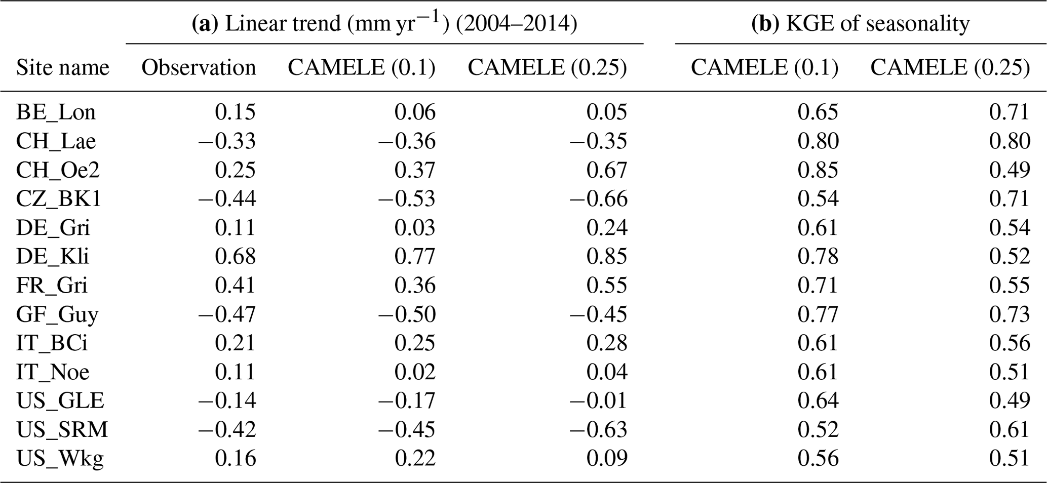
Furthermore, we present the linear trend estimated by CAMELE from 2004 to 2014 at 13 sites, along with the KGE values for monthly seasonality. The results indicate that, regardless of the resolution, whether 0.1° or 0.25°, the trends estimated by CAMELE are consistent with the observed trends, with minor differences. In comparison to the observed monthly seasonality, the KGE values exceed 0.5 at all the sites, with some sites exceeding 0.7, indicating that CAMELE can effectively capture the seasonal variations.
The results indicate that CAMELE effectively captures the multiyear changes in ET, but at 0.1°, it tends to overestimate seasonal fluctuations. We further generated global maps of multiyear linear trends in ET, estimating trends using the Theil–Sen slope method and testing significance with the Mann–Kendall method. The dotted areas indicate trends passing a significance test at a 5 % level.
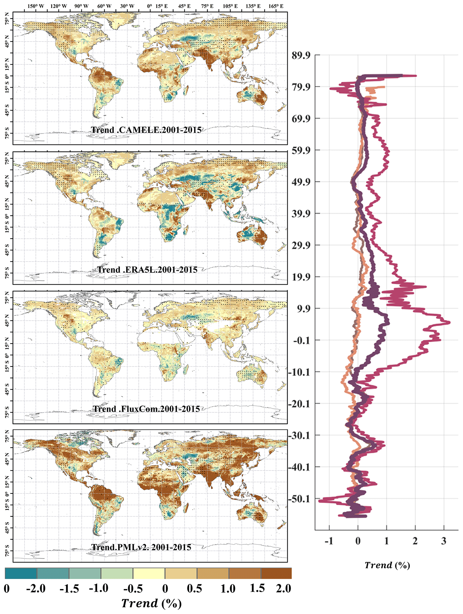
Figure 15Global distribution of the multiyear linear trend at 0.1° for CAMELE, ERA5L, FluxCom, and PMLv2, depicted alongside the corresponding average trend with latitude. The trend is estimated with the Theil–Sen slope method, and the significance level is tested with the Mann–Kendall method. The dotted area indicates that the trend has passed the significance test at the 5 % level.
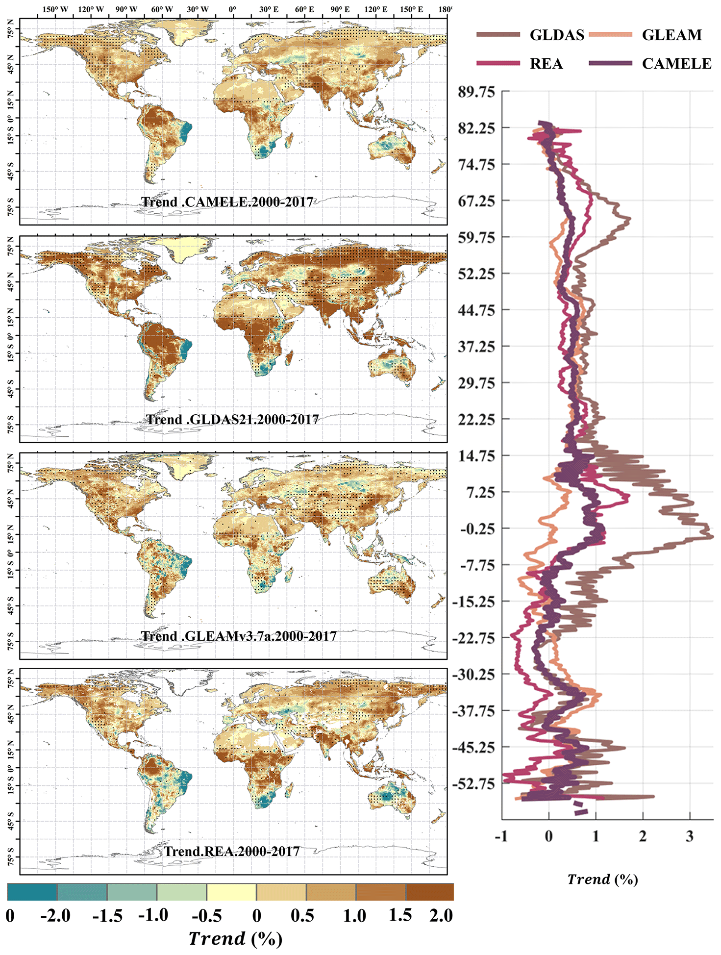
Figure 16Global distribution of the multiyear linear trend at 0.25° for CAMELE, GLDAS2.1, GLEAMv3.7a, and REA, depicted alongside the corresponding average trend with latitude. The trend is estimated with the Theil–Sen slope method, and the significance level is tested with the Mann–Kendall method. The dotted area indicates that the trend has passed the significance test at the 5 % level.
Figures 15 and 16 present the linear trends of multiyear daily-scale ET calculated for different products at resolutions of 0.1 and 0.25°, respectively. The corresponding latitude-dependent variations of the rate of change are shown on the right side. It can be observed that the differences in linear trends among the different products are more significant than the multiyear averages, and in some regions they even exhibit opposite trends. For example, at 0.1° resolution, PMLv2 shows a global increase of 1.0 % in ET in most regions, while the results from CAMELE, ERA5L, and PMLv2 indicate a milder increase in ET in the Amazon rainforest, southern Africa, and northwestern Australia. At 0.25° resolution, except for GLDAS2.1, which shows an apparent global increase in ET, the results from CAMELE, GLEAMv3.7a, and REA indicate milder variations in the global ET.
5.1 Impact of the underlying assumptions on the collocation analysis
The collocation analysis system relies on key assumptions, including linearity (linear regression model), stationarity (unchanged probability distribution over time), error orthogonality (independence between the random error and the true signal), and zero error cross-correlation (independence between random errors). Potential error autocorrelation is considered with lag-1 (day) series. Various studies have examined the validity and impact of these assumptions. Numerous studies have examined the validity of these assumptions and their impact on the outcomes if violated (Tsamalis, 2022; Duan et al., 2021; Gruber et al., 2020).
The linearity assumption shapes the error model by including additive and multiplicative biases and zero-mean random error. Although some studies have explored the application of a nonlinear rescaling technique (Yilmaz and Crow, 2013; Zwieback et al., 2016), those efforts are primarily limited to soil moisture signals and often fail to accurately represent the true signal unless all the datasets share a similar signal-to-noise ratio (SNR). However, it is worth noting that, after rescaling processes, such as cumulative distribution function (CDF) matching or climatology removal, the resulting time series (anomalies) are often considered linearly related to the truth since higher-order error terms are removed. In addition, multiplicative relationships have been more commonly identified in rainfall products (Li et al., 2018). In contrast, collocation analysis within the context of ET products frequently suggests that linear relationships are reasonable (Li et al., 2022; Park et al., 2023). Therefore, the linear error model remains a robust implementation, though it has the potential for improvement through rescaling techniques.
Regarding violating the stationarity assumption, the evapotranspiration signal does not strictly adhere to this characteristic. However, by collocating triplets with similar magnitude variations, the influence of this violation is minimized. Nonetheless, disparities in climatology between datasets can still arise for various reasons (Su and Ryu, 2015). Several proposed alternatives aim to address this issue, such as removing the climatology of inputs (Stoffelen, 1998; Yilmaz and Crow, 2014; Draper et al., 2013) and subsequently analyzing the random error variance of the anomalies (Dong et al., 2020b). Nevertheless, obtaining a reliable estimation of climatology proves challenging in practice.
The assumption of error orthogonality assumes independence between the random error and true signal, i.e., . A few studies have examined this assumption. Yilmaz and Crow (2014) investigated such violations using four in situ sites and concluded that the impact is negligible since rescaling mitigates or compensates for bias. Additionally, non-orthogonality results in non-zero ECC, although the latter is considered more important. Vogelzang et al. (2022) also investigated this violation recently and demonstrated minimal second-order impact.
Non-zero ECC conditions introduce more substantial bias in the results compared to other violations, mainly for two reasons: (1) they cannot be mitigated by rescaling; (2) they cannot be compensated even with equal magnitude for all inputs; and (3) they have been frequently reported in recent studies for various variables (Li et al., 2018, 2022; Gruber et al., 2016b). Gruber et al. (2016a) proposed the extended collocation method, which effectively addresses the ECC of selected pairs. Moreover, the EIVD method adopts the ECC framework. In the following section, we will analyze the ECC between pairs.
5.2 Analysis of error cross-correlation
This study assumes that non-zero ECC conditions exist between FluxCom and PMLv2 at 0.1° and between ERA5L and GLEAM at 0.25°. However, non-zero ECC conditions were also possible between other pairs. Therefore, we presented the EIVD-based ECC results of various pairs.
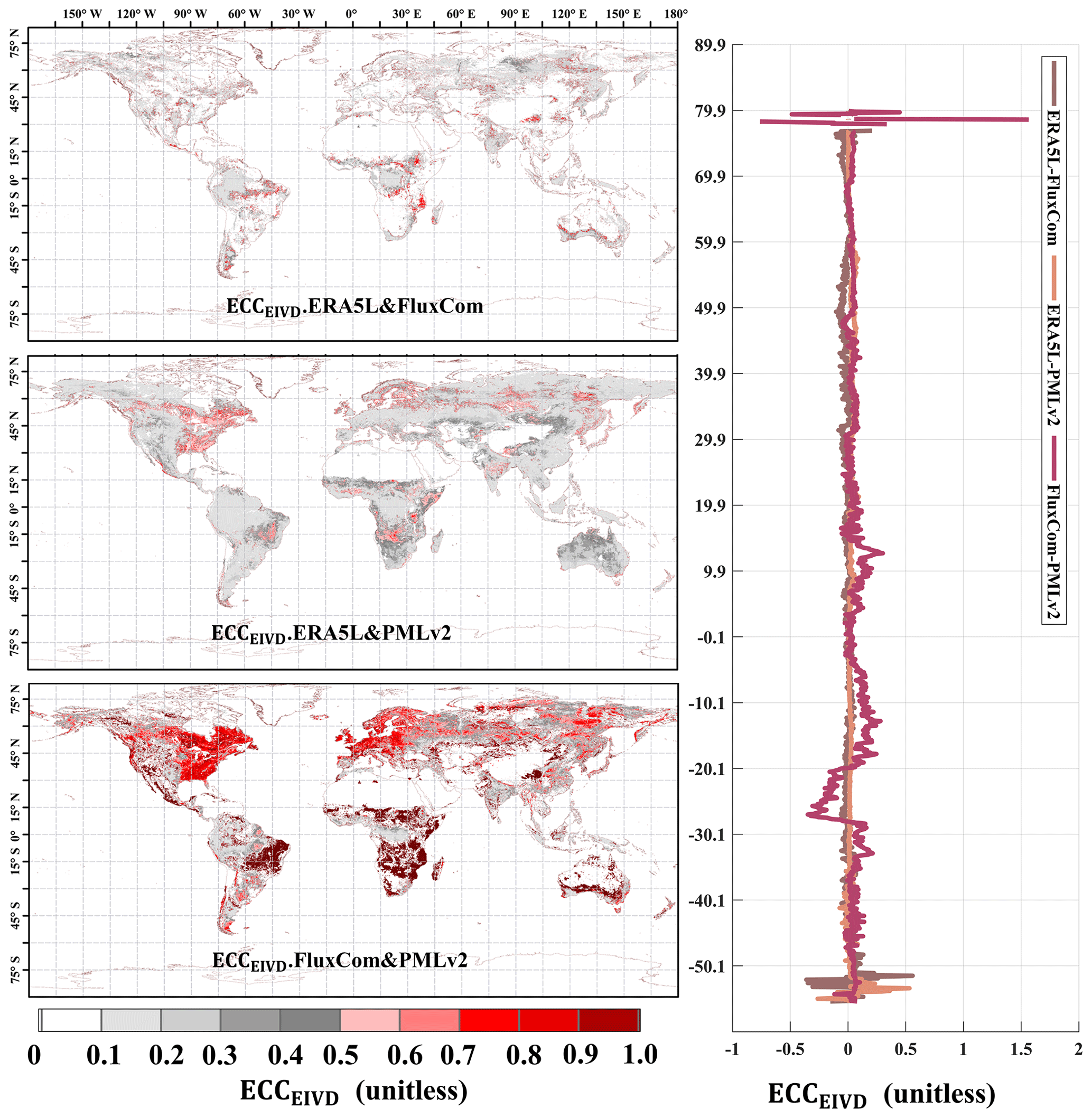
Figure 17Global distribution of the estimated error cross-correlation (ECC) between ERA5L, FluxCom, and PMLv2 pairwise using EIVD alongside relevant variation curves of the average with latitude.
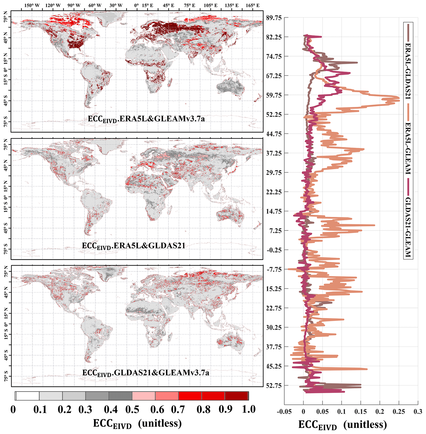
Figure 18Global distribution of the ECC between ERA5L, GLEAMv3.7a, and GLDAS21 pairwise using EIVD alongside the relevant variation curves of the average with latitude.
As depicted in Figs. 17 and 18, at a resolution of 0.1°, the ECC values of FluxCom and PMLv2 were notably higher than those of ERA5L–FluxCom and ERA5L–PMLv2. The global average ECC value for FluxCom–PMLv2 was 0.16, and regions with high ECC values were identified in the eastern United States, most of Europe, and the western Amazon, areas densely covered by measurement sites. Since both FluxCom and PMLv2 incorporated corrections based on FluxNet measurement sites, there is likely some overlap between the sites used by both products in the high-ECC regions. This partially explains the shared source of random errors between the two datasets.
The global error correlations of GLEAM–GLDAS and ERA5L–GLDAS are relatively low. The random error of ERA5L correlates with that of GLEAM, primarily in arid regions such as the Sahara, northwestern China, and central Australia, where the average ECC exceeds 0.20. The global average ECC of ERA5L–GLEAM is approximately 0.14. A higher error correlation is observed for ERA5L–GLEAM, with a mean ECC value of 0.26, which is expected since meteorological information from the ECMWF is reanalyzed for both datasets. However, ECC values for GLEAM–GLDAS and ERA5L–GLDAS are generally low globally, supporting the assumption of zero ECC for these two pairs.
Our findings highlight the significant impact of ECC between FluxCom–PMLv2 and ERA5L–GLEAM at the 0.1 and 0.25° resolutions, respectively. Mathematically, when a triplet exhibits a high ECC value (> 0.3) between two sets, it indicates a preference for the remaining independent product as the “better” one, potentially leading to an underestimation of its error variance. However, it is essential to note that the overall ECC values for other pairs are relatively small, suggesting that the zero ECC assumptions can be considered valid for these pairs across most areas. Therefore, these assumptions are unlikely to affect the relevant results of uncertainties significantly. Nevertheless, we have considered the non-zero ECC condition between FluxCom–PMLv2 and ERA5L–GLEAM in this study, as it requires careful consideration.
5.3 Comparison of different fusion schemes
In this section, we conducted comparisons in three aspects: (1) comparing the performance of CAMELE at different resolutions; (2) comparing the performance of different change fusion schemes, explicitly changing the input products' versions (GLDAS21 to GLDAS20 or GLDAS22, GLEAMv3.7a to v3.7b); and (3) comparing the performance of the results obtained without considering the ECC impact. We made a comprehensive comparison of our fusion approach with several alternative schemes. Specifically, these schemes encompassed utilization of only ERA5L and PMLV2 at 0.1° based on the IVD method (Comb1), changing the versions of GLDAS2 and GLEAM at 0.25° based on the EIVD method (Comb2–5), and two TC fusion approaches at 0.1 and 0.25°, which did not incorporate ECC.
It should be noted that the Comb2 scheme, which includes GLDAS20, covers the period from 1980 to 2014, while the other 0.25° comparison schemes (Comb3–5) span from 2003 to 2022. The combinations based on TC (assuming zero ECC) had the same inputs as CAMELE at both resolutions.
Table 8Average metrics for CAMELE and other fusion schemes at all the sites. The bold sections indicate the schemes with the best performance in their respective metrics.
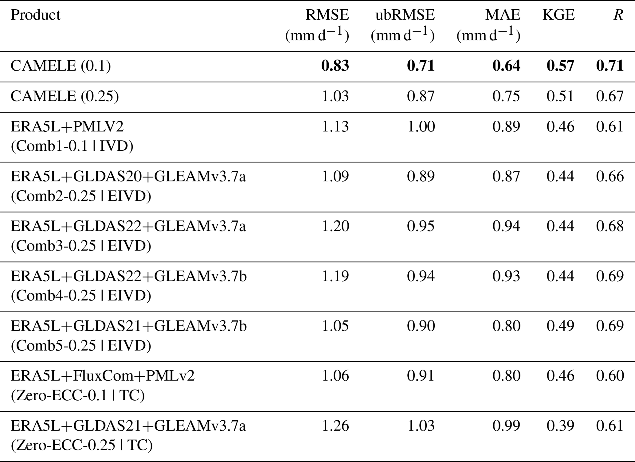
According to the information in the table, CAMELE (0.1°) results were superior in all the indicators. Firstly, when comparing the performance of CAMELE at resolutions of 0.1 and 0.25°, it was observed that the fused product performed slightly worse at the 0.25° resolution. Additionally, the representative of FluxNet sites at the 0.25° resolution decreased, leading to degraded statistical indicators.
At the 0.1° resolution, we conducted a comparison of results obtained by exclusively fusing ERA5-Land and PMLv2. Multiple indicators indicated that this approach did not enhance the accuracy of ET estimates and fell significantly short of the scheme employed in CAMELE. This implies that using only two product sets as input did not allow for effective error analysis through collocation analysis, resulting in suboptimal fusion results. More importantly, the limitation of employing only two datasets prevented us from effectively acquiring error information through collocation analysis (Dong et al., 2020a, 2019). Consequently, we made the strategic decision to ensure the inclusion of three datasets as inputs, facilitating the utilization of the EIVD method and maintaining methodological consistency between the 0.1 and 0.25° resolutions.
Furthermore, when comparing the results of different fusion schemes between CAMELE and Comb2–5 at the 0.25° resolution, CAMELE performed better regarding error metrics (RMSE, ubRMSE, MAE). The differences in the fitting metrics (KGE, R) were insignificant, indicating that the choice of fusion scheme primarily affected the errors of the fusion results. The relatively poorer performance of other fusion schemes could be due to the lack of consideration for non-zero ECC. For example, non-zero ECC between GLDAS-2.2 and ERA5L has been reported in a recent study (Li et al., 2023a).
For the comparative analysis of the GLDAS-2.0 and GLDAS-2.1 schemes, the usage of GLDAS-2.1 yielded better performance. The GLDAS-2.1 simulation leverages conditions from the GLDAS-2.0 simulation, with improved models driven by a combination of datasets. Previous research has demonstrated that GLDAS-2.1 offers improvements in the regional-scale simulation of hydrological variables compared to GLDAS-2.0 (Qi et al., 2018, 2020). Consequently, we chose to incorporate GLDAS-2.1 data for as much of the time series as possible.
Moreover, when comparing the fusion effects considering and not considering non-zero ECC conditions, it was evident that considering ECC information could effectively improve the performance of the fused product, which further demonstrated the reliability and advantages of the fusion method employed in this study.
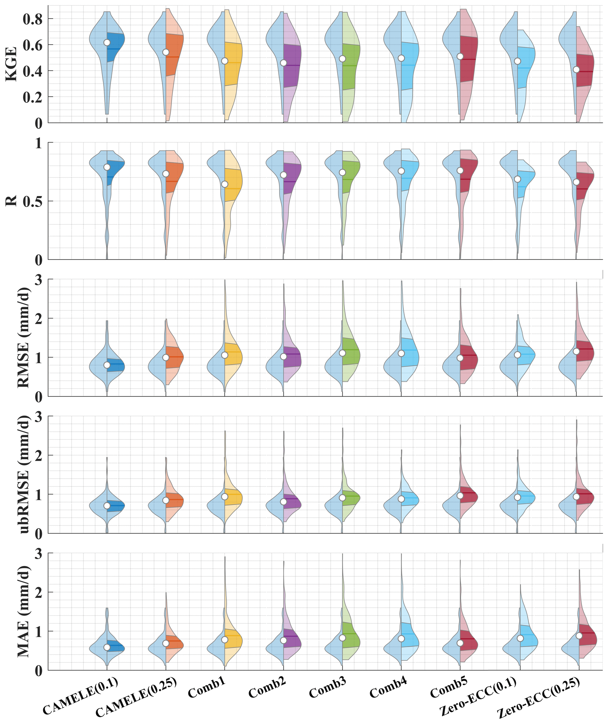
Figure 19Violin plot comparing the KGE, R, RMSE, ubRMSE, and MAE of CAMELE with other fusion schemes. The right half of each violin plot represents the distribution, with shaded areas indicating the box plot, where the horizontal line corresponds to the median and the dot represents the mean. The left half represents the results of CAMELE (0.1°) for comparison.
We further provided violin plots for different metrics, comparing the results of each fusion scheme to CAMELE (0.1°), as shown in Fig. 19. The results indicated that the fusion schemes adopted were significantly superior to other schemes based on the distribution of results for all the metrics across all the sites. Regarding KGE and R, CAMELE's results were concentrated near 1 for most of the sites. Regarding RMSE, ubRMSE, and MAE, their results were concentrated below 1 mm d−1. The results in the plots also suggested that CAMELE performed slightly worse at 0.25° compared to 0.1° but still outperformed other combination results. Additionally, comparing CAMELE and the zero-ECC scheme in the plots further highlighted the importance of considering non-zero ECC conditions.
5.4 Potential applications and future enhancements
In this section, we delve into the potential applications of our product and outline our commitment to future enhancements to maintain its accuracy and relevance.
Here, we identify three potential applications for our transpiration product. (1) Global ET trends: our product facilitates global-scale analysis of current ET patterns and long-term trends, essential for comprehending ecosystem responses to evolving environmental conditions in a warming climate. (2) Transpiration-to-evapotranspiration ratio: our merging approach can fuse multi-source global gridded transpiration data, allowing for the examination of the transpiration-to-evapotranspiration ratio. This analysis can enhance water resource management and water availability predictions in diverse regions. (3) Attribution analysis: our product is a valuable tool for attribution analysis, helping researchers identify the drivers of patterns. This knowledge is crucial for understanding the roles of climate variability, land-use changes, and other factors in shaping terrestrial water fluxes.
Furthermore, we are committed to enhancing our product proactively. Key strategies include the following. (1) Data update and validation: to ensure our product's continued accuracy and reliability, we will prioritize regularly updating the data used in this study to the latest versions. By adopting this approach, we aim to provide users with results that reflect the latest advancements in scientific knowledge. (2) Enhanced integration and error reduction: we continually refine estimates by incorporating additional data sources and implementing an extended collocation method to minimize errors. (3) Integration of high-resolution regional ET data: recognizing the significance of regional-scale insights, we will focus on improving the accuracy of CAMELE by integrating higher-resolution regional ET data. This integration will enable more precise regional estimation.
In summary, these endeavors collectively represent our commitment to maintaining our product's quality and relevance, ensuring its value to the scientific community.
The datasets utilized in this research can be accessed through the links provided in the dataset section. The CAMELE products are available at https://doi.org/10.5281/zenodo.5704736 (Li et al., 2023b). The data are distributed under a Creative Commons Attribution 4.0 License. Additionally, we provide example MATLAB codes to read and plot CAMELE data and employ the IVD and EIVD methods to merge the inputs. Please refer to the latest version, 202306.
This study used a collocation-based approach for merging data considering non-zero conditions. We successfully generated a long-term daily CAMELE evapotranspiration (ET) product at resolutions of 0.1° (2000 to 2020) and 0.25° (1980 to 2022) by integrating five widely used datasets: ERA5L, FluxCom, PMLv2, GLDAS, and GLEAM. The key findings of our study are as follows.
-
Collocation analysis methods proved to be a reliable tool for evaluating ET products without a reference dataset. This approach shows promising potential for error characterization, especially in regions with limited data availability or on a global scale. The evaluation results provided valuable insights into the data merging process.
-
Compared to five input products, REA, and SA, the CAMELE product performed well when evaluated against FluxNet flux tower data. While CAMELE may not excel in all individual metrics, it effectively reduces errors associated with the input products. The result showed Pearson correlation coefficients (R) of 0.63 and 0.65, root-mean-square errors (RMSEs) of 0.81 and 0.73 mm d−1, unbiased root-mean-square errors (ubRMSEs) of 1.20 and 1.04 mm d−1, mean absolute errors (MAEs) of 0.81 and 0.73 mm d−1, and Kling–Gupta efficiencies (KGEs) of 0.60 and 0.65 on average at resolutions of 0.1 and 0.25°, respectively. This robust performance is especially evident when assessing its comprehensive station-scale evaluation.
-
For different plant functional types (PFTs), the CAMELE product outperformed the five input products, REA, and SA in most PFTs. Although FluxCom and PMLv2 performed slightly better than CAMELE at some PFT sites, considering that both utilized FluxNet sites for product calibration, it indirectly demonstrates the promising and robust performance of CAMELE.
-
Based on site-scale observations, CAMELE effectively captures the multiyear linear trend of ET. The accuracy of the multiyear mean value depicted by CAMELE is improved compared to the input data. Moreover, it accurately characterizes extreme ET values. However, there is a slight overestimation in representing the seasonality, which needs further improvement in future research.
-
When utilizing the error information derived from collocation analysis for merging, it is crucial to consider the potential presence of non-zero ECC. Comparing the merging schemes with and without considering non-zero ECC, it was found that considering ECC improves the accuracy of the merging process. Additionally, when using collocation analysis, it is necessary to identify which products may have ECC in advance, providing more effective support for data merging and obtaining more accurate product error information.
In conclusion, our proposed collocation-based data merging approach demonstrates promising potential for merging ET products. The resulting CAMELE product exhibited good overall performance at site-based and regional scales, meeting the requirements for more detailed research. Furthermore, further evaluation of the merged product in specific regions is necessary to improve its accuracy. In future studies, dynamic weights could be computed by considering suitable merging periods for different products to enhance the quality of the merged product, and more sophisticated combination schemes could be explored to improve accuracy.
The supplement related to this article is available online at: https://doi.org/10.5194/essd-16-1811-2024-supplement.
CL conceived and designed the study, collected and analyzed the data, and wrote the manuscript. HY participated in the study design, provided intellectual insights, and reviewed the manuscript for important intellectual content. ZL and WY provided substantial input in the study design and data interpretation and revised the manuscript. ZT, JH, and SL guided the research process and critically reviewed the manuscript. All the authors read and approved the final version of the manuscript.
The contact author has declared that none of the authors has any competing interests.
Publisher's note: Copernicus Publications remains neutral with regard to jurisdictional claims made in the text, published maps, institutional affiliations, or any other geographical representation in this paper. While Copernicus Publications makes every effort to include appropriate place names, the final responsibility lies with the authors.
This research was supported by the China National Key R&D Program (grant no. 2022YFC3002802), the National Natural Science Foundation of China (grant nos. 51979140, 52309022, and 42041004), and the Key Research and Development Program of Yunnan Province, China (grant no. 202203AA080010).
This research was supported by the China National Key R&D Program (grant no. 2022YFC3002802), the National Natural Science Foundation of China (grant nos.51979140, 52309022 and 42041004), and the Key Research and Development Program of Yunnan Province, China (grant no. 202203AA080010).
This paper was edited by Di Tian and reviewed by three anonymous referees.
Baker, J. C. A., Garcia-Carreras, L., Gloor, M., Marsham, J. H., Buermann, W., da Rocha, H. R., Nobre, A. D., de Araujo, A. C., and Spracklen, D. V.: Evapotranspiration in the Amazon: spatial patterns, seasonality, and recent trends in observations, reanalysis, and climate models, Hydrol. Earth Syst. Sci., 25, 2279–2300, https://doi.org/10.5194/hess-25-2279-2021, 2021.
Barraza Bernadas, V., Grings, F., Restrepo-Coupe, N., and Huete, A.: Comparison of the performance of latent heat flux products over southern hemisphere forest ecosystems: estimating latent heat flux error structure using in situ measurements and the triple collocation method, Int. J. Remote Sens., 39, 6300–6315, 2018.
Bates, J. M. and Granger, C. W.: The combination of forecasts, J. Oper. Res. Soc., 20, 451–468, 1969.
Chen, Z., Zhu, Z., Jiang, H., and Sun, S.: Estimating daily reference evapotranspiration based on limited meteorological data using deep learning and classical machine learning methods, J. Hydrol., 591, 125286, https://doi.org/10.1016/j.jhydrol.2020.125286, 2020.
De Lannoy, G. J., Houser, P. R., Verhoest, N. E., Pauwels, V. R., and Gish, T. J.: Upscaling of point soil moisture measurements to field averages at the OPE3 test site, J. Hydrol., 343, 1–11, 2007.
Deng, X., Zhu, L., Wang, H., Zhang, X., Tong, C., Li, S., and Wang, K.: Triple Collocation Analysis and In Situ Validation of the CYGNSS Soil Moisture Product, IEEE J. Sel. Top. Appl., 16, 1883–1899, https://doi.org/10.1109/jstars.2023.3235111, 2023.
Dong, J. and Crow, W. T.: An Improved Triple Collocation Analysis Algorithm for Decomposing Autocorrelated and White Soil Moisture Retrieval Errors, J. Geophys. Res.-Atmos., 122, 13081–13094, https://doi.org/10.1002/2017jd027387, 2017.
Dong, J., Crow, W. T., Duan, Z., Wei, L., and Lu, Y.: A double instrumental variable method for geophysical product error estimation, Remote Sens. Environ., 225, 217–228, https://doi.org/10.1016/j.rse.2019.03.003, 2019.
Dong, J., Wei, L., Chen, X., Duan, Z., and Lu, Y.: An instrument variable based algorithm for estimating cross-correlated hydrological remote sensing errors, J. Hydrol., 581, 124413, https://doi.org/10.1016/j.jhydrol.2019.124413, 2020a.
Dong, J., Lei, F., and Wei, L.: Triple Collocation Based Multi-Source Precipitation Merging, Front. Water, 2, 498793, https://doi.org/10.3389/frwa.2020.00001, 2020b.
Dong, J., Crow, W. T., Chen, X., Tangdamrongsub, N., Gao, M., Sun, S., Qiu, J., Wei, L., Gao, H., and Duan, Z.: Statistical uncertainty analysis-based precipitation merging (SUPER): A new framework for improved global precipitation estimation, Remote Sens. Environ., 283, 113299, https://doi.org/10.1016/j.rse.2022.113299, 2022.
Draper, C., Reichle, R., de Jeu, R., Naeimi, V., Parinussa, R., and Wagner, W.: Estimating root mean square errors in remotely sensed soil moisture over continental scale domains, Remote Sens. Environ., 137, 288–298, 2013.
Duan, Z., Duggan, E., Chen, C., Gao, H., Dong, J., and Liu, J.: Comparison of traditional method and triple collocation analysis for evaluation of multiple gridded precipitation products across Germany, J. Hydrometeorol., 22, 2983–2999, https://doi.org/10.1175/JHM-D-21-0049.1, 2021.
ECMWF: In IFS documentation CY40R1 Part IV: Physical Processes, ECMWF, Reading, UK, 111–113, https://doi.org/10.21957/f56vvey1x, 2014.
Ershadi, A., McCabe, M. F., Evans, J. P., Chaney, N. W., and Wood, E. F.: Multi-site evaluation of terrestrial evaporation models using FLUXNET data, Agr. Forest Meteorol., 187, 46–61, https://doi.org/10.1016/j.agrformet.2013.11.008, 2014.
Feng, Y., Cui, N., Zhao, L., Hu, X., and Gong, D.: Comparison of ELM, GANN, WNN and empirical models for estimating reference evapotranspiration in humid region of Southwest China, J. Hydrol., 536, 376–383, https://doi.org/10.1016/j.jhydrol.2016.02.053, 2016.
Gan, R., Zhang, Y., Shi, H., Yang, Y., Eamus, D., Cheng, L., Chiew, F. H., and Yu, Q.: Use of satellite leaf area index estimating evapotranspiration and gross assimilation for Australian ecosystems, Ecohydrology, 11, e1974, https://doi.org/10.1002/eco.1974, 2018.
Gentine, P., Massmann, A., Lintner, B. R., Hamed Alemohammad, S., Fu, R., Green, J. K., Kennedy, D., and Vilà-Guerau de Arellano, J.: Land–atmosphere interactions in the tropics – a review, Hydrol. Earth Syst. Sci., 23, 4171–4197, https://doi.org/10.5194/hess-23-4171-2019, 2019.
Gruber, A., Su, C., Crow, W. T., Zwieback, S., Dorigo, W., and Wagner, W.: Estimating error cross-correlations in soil moisture data sets using extended collocation analysis, J. Geophys. Res.-Atmos., 121, 1208–1219, 2016a.
Gruber, A., Su, C.-H., Zwieback, S., Crow, W., Dorigo, W., and Wagner, W.: Recent advances in (soil moisture) triple collocation analysis, Int. J. Appl. Earth Obs., 45, 200–211, https://doi.org/10.1016/j.jag.2015.09.002, 2016b.
Gruber, A., Dorigo, W. A., Crow, W., and Wagner, W.: Triple Collocation-Based Merging of Satellite Soil Moisture Retrievals, IEEE Ts. Geosci. Remote, 55, 6780–6792, https://doi.org/10.1109/TGRS.2017.2734070, 2017.
Gruber, A., Scanlon, T., van der Schalie, R., Wagner, W., and Dorigo, W.: Evolution of the ESA CCI Soil Moisture climate data records and their underlying merging methodology, Earth Syst. Sci. Data, 11, 717–739, https://doi.org/10.5194/essd-11-717-2019, 2019.
Gruber, A., De Lannoy, G., Albergel, C., Al-Yaari, A., Brocca, L., Calvet, J. C., Colliander, A., Cosh, M., Crow, W., Dorigo, W., Draper, C., Hirschi, M., Kerr, Y., Konings, A., Lahoz, W., McColl, K., Montzka, C., Muñoz-Sabater, J., Peng, J., Reichle, R., Richaume, P., Rüdiger, C., Scanlon, T., van der Schalie, R., Wigneron, J. P., and Wagner, W.: Validation practices for satellite soil moisture retrievals: What are (the) errors?, Remote Sens. Environ., 244, 111806, https://doi.org/10.1016/j.rse.2020.111806, 2020.
Gupta, H. V., Kling, H., Yilmaz, K. K., and Martinez, G. F.: Decomposition of the mean squared error and NSE performance criteria: Implications for improving hydrological modelling, J. Hydrol., 377, 80–91, 2009.
Han, S. and Tian, F.: A review of the complementary principle of evaporation: from the original linear relationship to generalized nonlinear functions, Hydrol. Earth Syst. Sci., 24, 2269–2285, https://doi.org/10.5194/hess-24-2269-2020, 2020.
Hao, Y., Baik, J., and Choi, M.: Combining generalized complementary relationship models with the Bayesian Model Averaging method to estimate actual evapotranspiration over China, Agr. Forest Meteorol., 279, 107759, https://doi.org/10.1016/j.agrformet.2019.107759, 2019.
Hersbach, H., Bell, B., Berrisford, P., Hirahara, S., Horányi, A., Muñoz-Sabater, J., Nicolas, J., Peubey, C., Radu, R., Schepers, D., Simmons, A., Soci, C., Abdalla, S., Abellan, X., Balsamo, G., Bechtold, P., Biavati, G., Bidlot, J., Bonavita, M., Chiara, G., Dahlgren, P., Dee, D., Diamantakis, M., Dragani, R., Flemming, J., Forbes, R., Fuentes, M., Geer, A., Haimberger, L., Healy, S., Hogan, R. J., Hólm, E., Janisková, M., Keeley, S., Laloyaux, P., Lopez, P., Lupu, C., Radnoti, G., Rosnay, P., Rozum, I., Vamborg, F., Villaume, S., and Thépaut, J.: The ERA5 global reanalysis, Q. J. Roy. Meteor. Soc., 146, 1999–2049, https://doi.org/10.1002/qj.3803, 2020.
Hoareau, N., Portabella, M., Lin, W., Ballabrera-Poy, J., and Turiel, A.: Error characterization of sea surface salinity products using triple collocation analysis, IEEE T. Geosci. Remote, 56, 5160–5168, 2018.
Jia, Y., Li, C., Yang, H., Yang, W., and Liu, Z.: Assessments of three evapotranspiration products over China using extended triple collocation and water balance methods, J. Hydrol., 614, 128594, https://doi.org/10.1016/j.jhydrol.2022.128594, 2022.
Jiang, C. and Ryu, Y.: Multi-scale evaluation of global gross primary productivity and evapotranspiration products derived from Breathing Earth System Simulator (BESS), Remote Sens. Environ., 186, 528–547, 2016.
Jiang, C., Ryu, Y., Fang, H., Myneni, R., Claverie, M., and Zhu, Z.: Inconsistencies of interannual variability and trends in long-term satellite leaf area index products, Glob. Chang Biol., 23, 4133–4146, https://doi.org/10.1111/gcb.13787, 2017.
Jiang, C., Guan, K., Pan, M., Ryu, Y., Peng, B., and Wang, S.: BESS-STAIR: a framework to estimate daily, 30 m, and all-weather crop evapotranspiration using multi-source satellite data for the US Corn Belt, Hydrol. Earth Syst. Sci., 24, 1251–1273, https://doi.org/10.5194/hess-24-1251-2020, 2020.
Jiménez, C., Prigent, C., Mueller, B., Seneviratne, S. I., McCabe, M. F., Wood, E. F., Rossow, W. B., Balsamo, G., Betts, A. K., Dirmeyer, P. A., Fisher, J. B., Jung, M., Kanamitsu, M., Reichle, R. H., Reichstein, M., Rodell, M., Sheffield, J., Tu, K., and Wang, K.: Global intercomparison of 12 land surface heat flux estimates, J. Geophys. Res., 116, d014545, https://doi.org/10.1029/2010jd014545, 2011.
Jung, M., Koirala, S., Weber, U., Ichii, K., Gans, F., Camps-Valls, G., Papale, D., Schwalm, C., Tramontana, G., and Reichstein, M.: The FLUXCOM ensemble of global land-atmosphere energy fluxes, Sci. Data, 6, 74, https://doi.org/10.1038/s41597-019-0076-8, 2019.
Khan, M. S., Liaqat, U. W., Baik, J., and Choi, M.: Stand-alone uncertainty characterization of GLEAM, GLDAS and MOD16 evapotranspiration products using an extended triple collocation approach, Agr. Forest Meteorol., 252, 256–268, https://doi.org/10.1016/j.agrformet.2018.01.022, 2018.
Kim, S., Pham, H. T., Liu, Y. Y., Marshall, L., and Sharma, A.: Improving the Combination of Satellite Soil Moisture Data Sets by Considering Error Cross Correlation: A Comparison Between Triple Collocation (TC) and Extended Double Instrumental Variable (EIVD) Alternatives, IEEE T. Geosci. Remote, 59, 7285–7295, https://doi.org/10.1109/tgrs.2020.3032418, 2021a.
Kim, S., Sharma, A., Liu, Y. Y., and Young, S. I.: Rethinking satellite data merging: from averaging to SNR optimization, IEEE T. Geosci. Remote, 60, 1–15, 2021b.
Kling, H., Fuchs, M., and Paulin, M.: Runoff conditions in the upper Danube basin under an ensemble of climate change scenarios, J. Hydrol., 424–425, 264–277, https://doi.org/10.1016/j.jhydrol.2012.01.011, 2012.
Knauer, J., Zaehle, S., Medlyn, B. E., Reichstein, M., Williams, C. A., Migliavacca, M., De Kauwe, M. G., Werner, C., Keitel, C., Kolari, P., Limousin, J. M., and Linderson, M. L.: Towards physiologically meaningful water-use efficiency estimates from eddy covariance data, Glob. Chang Biol., 24, 694–710, https://doi.org/10.1111/gcb.13893, 2018.
Knoben, W. J. M., Freer, J. E., and Woods, R. A.: Technical note: Inherent benchmark or not? Comparing Nash–Sutcliffe and Kling–Gupta efficiency scores, Hydrol. Earth Syst. Sci., 23, 4323–4331, https://doi.org/10.5194/hess-23-4323-2019, 2019.
Koster, R. D., Liu, Q., Reichle, R. H., and Huffman, G. J.: Improved Estimates of Pentad Precipitation Through the Merging of Independent Precipitation Data Sets, Water Resour. Res., 57, e2021WR030330, https://doi.org/10.1029/2021wr030330, 2021.
Leuning, R., Zhang, Y., Rajaud, A., Cleugh, H., and Tu, K.: A simple surface conductance model to estimate regional evaporation using MODIS leaf area index and the Penman-Monteith equation, Water Resour. Res., 44, W10419, https://doi.org/10.1029/2007WR006562, 2008.
Leuning, R., Zhang, Y. Q., Rajaud, A., Cleugh, H., and Tu, K.: Correction to “A simple surface conductance model to estimate regional evaporation using MODIS leaf area index and the Penman-Monteith equation,” Water Resour. Res., 45, W01701, https://doi.org/10.1029/2008wr007631, 2009.
Li, B., Rodell, M., Kumar, S., Beaudoing, H. K., Getirana, A., Zaitchik, B. F., Goncalves, L. G., Cossetin, C., Bhanja, S., Mukherjee, A., Tian, S., Tangdamrongsub, N., Long, D., Nanteza, J., Lee, J., Policelli, F., Goni, I. B., Daira, D., Bila, M., Lannoy, G., Mocko, D., Steele-Dunne, S. C., Save, H., and Bettadpur, S.: Global GRACE Data Assimilation for Groundwater and Drought Monitoring: Advances and Challenges, Water Resour. Res., 55, 7564–7586, https://doi.org/10.1029/2018WR024618, 2019.
Li, C., Tang, G., and Hong, Y.: Cross-evaluation of ground-based, multi-satellite and reanalysis precipitation products: Applicability of the Triple Collocation method across Mainland China, J. Hydrol., 562, 71–83, https://doi.org/10.1016/j.jhydrol.2018.04.039, 2018.
Li, C., Yang, H., Yang, W., Liu, Z., Jia, Y., Li, S., and Yang, D.: Error Characterization of Global Land Evapotranspiration Products: Collocation-based approach, J. Hydrol., 612, 128102, https://doi.org/10.1016/j.jhydrol.2022.128102, 2022.
Li, C., Liu, Z., Tu, Z., Shen, J., He, Y., and Yang, H.: Assessment of global gridded transpiration products using the extended instrumental variable technique (EIVD), J. Hydrol., 623, 129880, https://doi.org/10.1016/j.jhydrol.2023.129880, 2023a.
Li, C., Liu, Z., Yang, W., Tu, Z., Han, J., Sien, L., and Hanbo, Y.: CAMELE: Collocation-Analyzed Multi-source Ensembled Land Evapotranspiration Data, Zenodo [data set], https://doi.org/10.5281/zenodo.8047038, 2023b.
Li, X., Gentine, P., Lin, C., Zhou, S., Sun, Z., Zheng, Y., Liu, J., and Zheng, C.: A simple and objective method to partition evapotranspiration into transpiration and evaporation at eddy-covariance sites, Agr. Forest Meteorol., 265, 171–182, https://doi.org/10.1016/j.agrformet.2018.11.017, 2019.
Li, X., Zhang, W., Vermeulen, A., Dong, J., and Duan, Z.: Triple collocation-based merging of multi-source gridded evapotranspiration data in the Nordic Region, Agr. Forest Meteorol., 335, 109451, https://doi.org/10.1016/j.agrformet.2023.109451, 2023.
Lian, X., Piao, S., Huntingford, C., Li, Y., Zeng, Z., Wang, X., Ciais, P., McVicar, T. R., Peng, S., Ottlé, C., Yang, H., Yang, Y., Zhang, Y., and Wang, T.: Partitioning global land evapotranspiration using CMIP5 models constrained by observations, Nat. Clim. Change, 8, 640–646, https://doi.org/10.1038/s41558-018-0207-9, 2018.
Lin, C., Gentine, P., Huang, Y., Guan, K., Kimm, H., and Zhou, S.: Diel ecosystem conductance response to vapor pressure deficit is suboptimal and independent of soil moisture, Agr. Forest Meteorol., 250, 24–34, 2018.
Loveland, T. R., Zhu, Z., Ohlen, D. O., Brown, J. F., Reed, B. C., and Yang, L.: An analysis of the IGBP global land-cover characterization process, Photogramm. Eng. Remote S., 65, 1021–1032, 1999.
Lu, J., Wang, G., Chen, T., Li, S., Hagan, D. F. T., Kattel, G., Peng, J., Jiang, T., and Su, B.: A harmonized global land evaporation dataset from model-based products covering 1980–2017, Earth Syst. Sci. Data, 13, 5879–5898, https://doi.org/10.5194/essd-13-5879-2021, 2021.
Ma, N., Szilagyi, J., and Jozsa, J.: Benchmarking large-scale evapotranspiration estimates: A perspective from a calibration-free complementary relationship approach and FLUXCOM, J. Hydrol., 590, 125221, https://doi.org/10.1016/j.jhydrol.2020.125221, 2020.
Majozi, N. P., Mannaerts, C. M., Ramoelo, A., Mathieu, R., Nickless, A., and Verhoef, W.: Analysing surface energy balance closure and partitioning over a semi-arid savanna FLUXNET site in Skukuza, Kruger National Park, South Africa, Hydrol. Earth Syst. Sci., 21, 3401–3415, https://doi.org/10.5194/hess-21-3401-2017, 2017.
Martens, B., Miralles, D. G., Lievens, H., van der Schalie, R., de Jeu, R. A. M., Fernández-Prieto, D., Beck, H. E., Dorigo, W. A., and Verhoest, N. E. C.: GLEAM v3: satellite-based land evaporation and root-zone soil moisture, Geosci. Model Dev., 10, 1903–1925, https://doi.org/10.5194/gmd-10-1903-2017, 2017.
McColl, K. A., Vogelzang, J., Konings, A. G., Entekhabi, D., Piles, M., and Stoffelen, A.: Extended triple collocation: Estimating errors and correlation coefficients with respect to an unknown target, Geophys. Res. Lett., 41, 6229–6236, https://doi.org/10.1002/2014gl061322, 2014.
Medlyn, B. E., De Kauwe, M. G., Lin, Y. S., Knauer, J., Duursma, R. A., Williams, C. A., Arneth, A., Clement, R., Isaac, P., Limousin, J. M., Linderson, M. L., Meir, P., Martin-StPaul, N., and Wingate, L.: How do leaf and ecosystem measures of water-use efficiency compare?, New Phytol., 216, 758–770, https://doi.org/10.1111/nph.14626, 2017.
Ming, W., Ji, X., Zhang, M., Li, Y., Liu, C., Wang, Y., and Li, J.: A Hybrid Triple Collocation-Deep Learning Approach for Improving Soil Moisture Estimation from Satellite and Model-Based Data, Remote Sens., 14, 1744, https://doi.org/10.3390/rs14071744, 2022.
Miralles, D. G., De Jeu, R. A. M., Gash, J. H., Holmes, T. R. H., and Dolman, A. J.: Magnitude and variability of land evaporation and its components at the global scale, Hydrol. Earth Syst. Sci., 15, 967–981, https://doi.org/10.5194/hess-15-967-2011, 2011.
Miralles, D. G., Gentine, P., Seneviratne, S. I., and Teuling, A. J.: Land-atmospheric feedbacks during droughts and heatwaves: state of the science and current challenges, Ann. NY Acad. Sci., 1436, 19–35, https://doi.org/10.1111/nyas.13912, 2019.
Mu, Q., Zhao, M., and Running, S. W.: Improvements to a MODIS global terrestrial evapotranspiration algorithm, Remote Sens. Environ., 115, 1781–1800, 2011.
Muñoz-Sabater, J., Dutra, E., Agustí-Panareda, A., Albergel, C., Arduini, G., Balsamo, G., Boussetta, S., Choulga, M., Harrigan, S., Hersbach, H., Martens, B., Miralles, D. G., Piles, M., Rodríguez-Fernández, N. J., Zsoter, E., Buontempo, C., and Thépaut, J.-N.: ERA5-Land: a state-of-the-art global reanalysis dataset for land applications, Earth Syst. Sci. Data, 13, 4349–4383, https://doi.org/10.5194/essd-13-4349-2021, 2021.
Pan, S., Pan, N., Tian, H., Friedlingstein, P., Sitch, S., Shi, H., Arora, V. K., Haverd, V., Jain, A. K., Kato, E., Lienert, S., Lombardozzi, D., Nabel, J. E. M. S., Ottlé, C., Poulter, B., Zaehle, S., and Running, S. W.: Evaluation of global terrestrial evapotranspiration using state-of-the-art approaches in remote sensing, machine learning and land surface modeling, Hydrol. Earth Syst. Sci., 24, 1485–1509, https://doi.org/10.5194/hess-24-1485-2020, 2020.
Park, J., Baik, J., and Choi, M.: Triple collocation-based multi-source evaporation and transpiration merging, Agr. Forest Meteorol., 331, 109353, https://doi.org/10.1016/j.agrformet.2023.109353, 2023.
Pastorello, G., Trotta, C., Canfora, E., Chu, H., Christianson, D., Cheah, Y.-W., Poindexter, C., Chen, J., Elbashandy, A., and Humphrey, M.: The FLUXNET2015 dataset and the ONEFlux processing pipeline for eddy covariance data, Sci. Data, 7, 225, https://doi.org/10.1038/s41597-020-0534-3, 2020.
Priestley, C. H. B. and Taylor, R. J.: On the assessment of surface heat flux and evaporation using large-scale parameters, Mon. Weather Rev., 100, 81–92, 1972.
Qi, W., Liu, J., and Chen, D.: Evaluations and Improvements of GLDAS2.0 and GLDAS2.1 Forcing Data's Applicability for Basin Scale Hydrological Simulations in the Tibetan Plateau, J. Geophys. Res.-Atmos., 123, 13128–13148, https://doi.org/10.1029/2018JD029116, 2018.
Qi, W., Liu, J., Yang, H., Zhu, X., Tian, Y., Jiang, X., Huang, X., and Feng, L.: Large Uncertainties in Runoff Estimations of GLDAS Versions 2.0 and 2.1 in China, Earth Space Sci., 7, e2019EA000829, https://doi.org/10.1029/2019EA000829, 2020.
Restrepo-Coupe, N., Albert, L. P., Longo, M., Baker, I., Levine, N. M., Mercado, L. M., da Araujo, A. C., Christoffersen, B. O., Costa, M. H., Fitzjarrald, D. R., Galbraith, D., Imbuzeiro, H., Malhi, Y., von Randow, C., Zeng, X., Moorcroft, P., and Saleska, S. R.: Understanding water and energy fluxes in the Amazonia: Lessons from an observation-model intercomparison, Glob. Change Biol., 27, 1802–1819, https://doi.org/10.1111/gcb.15555, 2021.
Ribal, A. and Young, I. R.: Global Calibration and Error Estimation of Altimeter, Scatterometer, and Radiometer Wind Speed Using Triple Collocation, Remote Sens., 12, https://doi.org/10.3390/rs12121997, 2020.
Rodell, M., Houser, P., Jambor, U., Gottschalck, J., Mitchell, K., Meng, C.-J., Arsenault, K., Cosgrove, B., Radakovich, J., and Bosilovich, M.: The global land data assimilation system, B. Am. Meteorol. Soc., 85, 381–394, 2004.
Sheffield, J., Goteti, G., and Wood, E. F.: Development of a 50-Year High-Resolution Global Dataset of Meteorological Forcings for Land Surface Modeling, J. Climate, 19, 3088–3111, https://doi.org/10.1175/JCLI3790.1, 2006.
Stoffelen, A.: Toward the true near-surface wind speed: Error modeling and calibration using triple collocation, J. Geophys. Res.-Oceans, 103, 7755–7766, https://doi.org/10.1029/97jc03180, 1998.
Su, C.-H. and Ryu, D.: Multi-scale analysis of bias correction of soil moisture, Hydrol. Earth Syst. Sci., 19, 17–31, https://doi.org/10.5194/hess-19-17-2015, 2015.
Su, C.-H., Ryu, D., Crow, W. T., and Western, A. W.: Beyond triple collocation: Applications to soil moisture monitoring, J. Geophys. Res.-Atmos., 119, 6419–6439, https://doi.org/10.1002/2013jd021043, 2014.
Sun, J., McColl, K. A., Wang, Y., Rigden, A. J., Lu, H., Yang, K., Li, Y., and Santanello, J. A.: Global evaluation of terrestrial near-surface air temperature and specific humidity retrievals from the Atmospheric Infrared Sounder (AIRS), Remote Sens. Environ., 252, 112146, https://doi.org/10.1016/j.rse.2020.112146, 2021.
Towner, J., Cloke, H. L., Zsoter, E., Flamig, Z., Hoch, J. M., Bazo, J., Coughlan de Perez, E., and Stephens, E. M.: Assessing the performance of global hydrological models for capturing peak river flows in the Amazon basin, Hydrol. Earth Syst. Sci., 23, 3057–3080, https://doi.org/10.5194/hess-23-3057-2019, 2019.
Tsamalis, C.: Clarifications on the equations and the sample number in triple collocation analysis using SST observations, Remote Sens. Environ., 272, 112936, https://doi.org/10.1016/j.rse.2022.112936, 2022.
Twine, T. E., Kustas, W., Norman, J., Cook, D., Houser, Pr., Meyers, T., Prueger, J., Starks, P., and Wesely, M.: Correcting eddy-covariance flux underestimates over a grassland, Agr. Forest Meteorol., 103, 279–300, 2000.
Vogelzang, J., Stoffelen, A., and Verhoef, A.: The Effect of Error Non-Orthogonality on Triple Collocation Analyses, Remote Sens., 14, 4268, https://doi.org/10.3390/rs14174268, 2022.
Wu, K., Ryu, D., Nie, L., and Shu, H.: Time-variant error characterization of SMAP and ASCAT soil moisture using Triple Collocation Analysis, Remote Sens. Environ., 256, 112324, https://doi.org/10.1016/j.rse.2021.112324, 2021.
Yang, Y., Roderick, M. L., Guo, H., Miralles, D. G., Zhang, L., Fatichi, S., Luo, X., Zhang, Y., McVicar, T. R., and Tu, Z.: Evapotranspiration on a greening Earth, Nat. Rev. Earth Environ., 4, 626–641, 2023.
Yilmaz, M. T. and Crow, W. T.: The optimality of potential rescaling approaches in land data assimilation, J. Hydrometeorol., 14, 650–660, 2013.
Yilmaz, M. T. and Crow, W. T.: Evaluation of Assumptions in Soil Moisture Triple Collocation Analysis, J. Hydrometeorol., 15, 1293–1302, https://doi.org/10.1175/JHM-D-13-0158.1, 2014.
Yilmaz, M. T., Crow, W. T., Anderson, M. C., and Hain, C.: An objective methodology for merging satellite- and model-based soil moisture products, Water Resour. Res., 48, W11502, https://doi.org/10.1029/2011wr011682, 2012.
Yin, G. and Park, J.: The use of triple collocation approach to merge satellite- and model-based terrestrial water storage for flood potential analysis, J. Hydrol., 603, 127197, https://doi.org/10.1016/j.jhydrol.2021.127197, 2021.
Yin, L., Tao, F., Chen, Y., Liu, F., and Hu, J.: Improving terrestrial evapotranspiration estimation across China during 2000–2018 with machine learning methods, J. Hydrol., 600, 126538, https://doi.org/10.1016/j.jhydrol.2021.126538, 2021.
Zhang, Y., Leuning, R., Hutley, L. B., Beringer, J., McHugh, I., and Walker, J. P.: Using long-term water balances to parameterize surface conductances and calculate evaporation at 0.05 spatial resolution, Water Resour. Res., 46, W05512, https://doi.org/10.1029/2009WR008716, 2010.
Zhang, Y., Kong, D., Gan, R., Chiew, F. H. S., McVicar, T. R., Zhang, Q., and Yang, Y.: Coupled estimation of 500 m and 8-day resolution global evapotranspiration and gross primary production in 2002–2017, Remote Sens. Environ., 222, 165–182, https://doi.org/10.1016/j.rse.2018.12.031, 2019.
Zhao, M., Liu, Y., and Konings, A. G.: Evapotranspiration frequently increases during droughts, Nat. Clim. Change, 12, 1024–1030, https://doi.org/10.1038/s41558-022-01505-3, 2022.
Zhu, G., Li, X., Zhang, K., Ding, Z., Han, T., Ma, J., Huang, C., He, J., and Ma, T.: Multi-model ensemble prediction of terrestrial evapotranspiration across north China using Bayesian model averaging, Hydrol. Process., 30, 2861–2879, https://doi.org/10.1002/hyp.10832, 2016.
Zwieback, S., Su, C.-H., Gruber, A., Dorigo, W. A., and Wagner, W.: The impact of quadratic nonlinear relations between soil moisture products on uncertainty estimates from triple collocation analysis and two quadratic extensions, J. Hydrometeorol., 17, 1725–1743, 2016.