the Creative Commons Attribution 4.0 License.
the Creative Commons Attribution 4.0 License.
 | 05 Apr 2024
Enriching the GEOFON seismic catalog with automatic energy magnitude estimations
Riccardo Zaccarelli
Angelo Strollo
Domenico Di Giacomo
Andres Heinloo
Peter Evans
Fabrice Cotton
Frederik Tilmann
We present a seismic catalog (Bindi et al., 2024, https://doi.org/10.5880/GFZ.2.6.2023.010) including energy magnitude Me estimated from P waves recorded at teleseismic distances in the range and for depths shorter than 80 km. The catalog is built starting from the event catalog disseminated by GEOFON (GEOFOrschungsNetz), considering 6349 earthquakes with moment magnitude Mw≥5 occurring between 2011 and 2023. Magnitudes are computed using 1 031 396 freely available waveforms archived in EIDA (European Integrated Data Archive) and IRIS (Incorporated Research Institutions for Seismology) repositories, retrieved through the standard International Federation of Digital Seismograph Networks (FDSN) web services (https://www.fdsn.org/webservices/, last access: March 2024). A reduced, high-quality catalog for events with Mw≥5.8 and from which stations and events with only few recordings were removed forms the basis of a detailed analysis of the residuals of individual station measurements, which are decomposed into station- and event-specific terms and a term accounting for remaining variability. The derived Me values are compared to Mw computed by GEOFON and with the Me values calculated by IRIS. Software and tools developed for downloading and processing waveforms for bulk analysis and an add-on for SeisComP for real-time assessment of Me in a monitoring context are also provided alongside the catalog. The SeisComP add-on has been part of the GEOFON routine processing since December 2021 to compute and disseminate Me for major events via the existing services.
- Article
(15427 KB) - Full-text XML
- BibTeX
- EndNote


Several magnitude scales have been defined to characterize the size of an earthquake. We can, however, divide magnitude scales in two groups, with one including magnitudes based on the amplitudes and periods of different seismic phases measured on band-limited signals (e.g., the body and surface wave magnitudes; Gutenberg, 1945a, b) and the other including magnitude scales related to estimations of macroscopic physical parameters of the earthquake source. The latter comprise the moment (Mw; Kanamori, 1977; Hanks and Kanamori, 1979) and the energy (Me; Boatwright and Choy, 1986) magnitudes, which are based on seismic moment (Aki, 1966) and radiated seismic energy (Haskell, 1964), respectively. These two magnitude scales are somewhat complementary because, although both represent an estimation of earthquake-related energy, they are determined by different parts of the source spectrum. The seismic moment extrapolated from the low-frequency end and represents the release of elastic energy stored in the Earth's crust or mantle being proportional to the integrated slip across the fault surface. The radiated seismic energy describes the fraction of the total energy released being radiated as seismic waves across all frequencies; i.e., it depends on the earthquake dynamics such as rupture velocity but also stress drop. Me estimates have been shown to play an important role when used in conjunction with Mw to better characterize the tsunami and shaking potential of an earthquake (Newman and Okal, 1998; Di Giacomo et al., 2010).
Mw is routinely computed from long period signals of broadband recordings, and it has become a robust and reliable source parameter for large and moderate earthquakes worldwide (Di Giacomo et al., 2021). On the other hand, the computation of Me is hindered by the necessity of integrating the velocity power spectra over a wide frequency range, while using signals in a limited bandwidth and taking into account propagation effects at high frequencies.
Aiming at validating and testing the procedures for operational purposes, we present a seismic catalog of Me computed, following the methodology proposed by Di Giacomo et al. (2008) and Di Giacomo et al. (2010) for the rapid assessment of energy magnitude (i.e., without requiring additional source information other than the hypocentral location). The approach is based on the analysis of spectra computed for teleseismic vertical component P waveforms. Teleseismic P waves are commonly used to compute Me for global earthquakes, as their energy loss during propagation can be more reliably modeled compared to S waves. We further present a detailed analysis of the residuals in a reduced high-quality catalog for events with Mw≥5.8 with respect to the Mw available in the GEOFON (GEOFOrschungsNetz) catalog and the Me values computed by IRIS.
2.1 Single-station estimation
We implement the methodology proposed by Di Giacomo et al. (2008) and Di Giacomo et al. (2010) to compute Me. Teleseismic vertical component P waveforms (BHZ channels, where B stands for broadband, H for high-gain seismometer, and Z for vertical component) are analyzed in the distance range from 20° to 98° and for earthquakes shallower than 80 km. Standard teleseismic range usually starts at 30°, but we use 20° to allow closer stations to be used for rapid response purposes. Shorter distances, however, are difficult to include for global earthquakes, as regional effects are not well accounted for with a 1-D model. Propagation effects are accounted for by frequency-dependent amplitude decay functions that are computed numerically (Wang, 1999) for the ak135Q model (Kennett et al., 1995; Montagner and Kennett, 1996) in the frequency range 0.012–1 Hz.
An estimate of radiated seismic energy Es is obtained for each single station from the integral of the power spectra of the vertical component P waveform, which is corrected for propagation effects (Haskell, 1964):
where α, β, and ρ are the P-wave velocity, S-wave velocity, and the density at the source, respectively. f is the frequency, and f1=0.012 Hz and f2=1 Hz are the lower and upper limits of the considered spectral bandwidth. is the P-wave velocity spectrum. G(f) is the median value of Green's function spectrum for displacement, computed from multiple combinations of focal mechanisms and varying strike, dip, and rake over a regular grid (Di Giacomo et al., 2008).
We used analysis windows starting 10 s before the P arrival and with lengths of 90 s for Mw≤7.5, 120 s for , and 180 s for Mw>8.5. The energy magnitude Me estimate for a single-event station pair is in turn computed as , with Es given in joules (Bormann et al., 2002). The procedure provides Me estimates at each recording station that can be averaged to minimize path-specific deviations not accounted for by the theoretical model (e.g., directivity and focal mechanism effects and regional variations in attenuation).
2.2 Open-source tool for computing Me
The above procedure is implemented in the package me-compute (Zaccarelli, 2023). The program uses stream2segment (Zaccarelli et al., 2019; Zaccarelli, 2018) to download events, station metadata, and waveforms from International Federation of Digital Seismograph Networks (FDSN)-compliant repositories in a structured query language (SQL) database.
In our application, the download is configured to fetch events from the GEOFON (Quinteros et al., 2021) event web service, selecting events with computed Mw in the time span 2011–2023. Waveforms are download from EIDA (Strollo et al., 2021) and IRIS (https://service.iris.edu/, last access: March 2024) data centers. The processing routine is implemented in a Python module, which computes the station energy magnitude for each downloaded waveform segment, as summarized in Sect. 2.1, and then calculates the event energy magnitude Me as the mean of all station magnitudes within the 5th–95th percentile range.
The final output consists of the following files:
-
a tabular file in a hierarchical data format (HDF), where each row represents the metadata and measurements, specifically also the station energy magnitude estimate, for a single waveform;
-
a tabular file in a comma-separated value (CSV) format aggregating the results of the previous file, where each row represents a seismic event, reporting the event data end metadata and including the Me estimate for the event;
-
an HTML (HyperText Markup Language) file visualizing the selected content reported in the CSV file, where the information for each event can be visualized on an interactive map; and
-
one file per processed event in the Quake Markup Language (QuakeML) format, where we also included the Me value.
All files produced by me-compute are disseminated in the data archive (Bindi et al., 2024; https://doi.org/10.5880/GFZ.2.6.2023.010), along with the stream2segment and me-compute configuration files.
We use me-compute to compute Me for Mw≥5 earthquakes since 2011 in the GEOFON catalog. Table 1 summarizes the steps followed to compile the disseminated Me catalog. The catalog reports the single-waveform energy magnitude Meij estimated at station j for earthquake i. The energy magnitude Me for each considered event i is then computed as the median of Meij over the set of recording stations, without considering station static corrections. The starting dataset D0 consists of more than 1 000 000 waveforms (channels BHZ) generated by 6963 earthquakes recorded by 7765 stations belonging to 246 different networks. Only recordings with an average signal-to-noise ratio (SNR) for the amplitude greater than 3 within the frequency range of interest are included in D0. Several integrity and quality checks are applied to remove outliers and faulty signals. Dataset D1 is obtained by analyzing the median residual at the network level, discarding 14 networks characterized by median residuals outside the 2.5 and 97.5 percentile range (Fig. 1a). Dataset D2 is then generated by analyzing the station median values and excluding 382 stations with residuals outside the 2.5–97.5 percentile range (Fig. 1b). Most of the networks and stations removed will have instrumental problems or faulty metadata regarding instrument responses, although in some cases stations with very strong site effects might also be excluded.
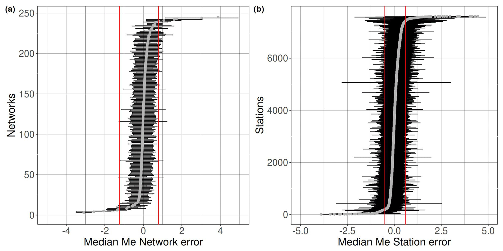
Figure 1Median network residuals (circles) for dataset D0 (a) and median station residuals for dataset D1 (b). Red lines correspond to the 2.5 and 97.5 percentiles of the distributions. For each network (a) and station (b), the horizontal bars correspond to the interval median (circle) ±1 median absolute deviation (MAD). A few values falling outside the range considered for the horizontal axis are not shown.
An anomaly score is computed to further refine the dataset by flagging anomalous amplitudes using the software sdaas (Zaccarelli, 2022). The software, developed from the work of Zaccarelli et al. (2021), is based on a machine learning algorithm specifically designed for outlier detection (Isolation Forest) which computes an anomaly score in [0,1], representing the degree of belief of a waveform to be an outlier. The score can be used to assign robustness weights or to define thresholds above which data can be discarded. After inspecting the distribution of the anomaly scores, we set the threshold to 0.62 for Mw<7.5 and to 0.80 for Mw≥7.5.
The spatial distribution of events and stations generating dataset D3 (Bindi et al., 2024) are shown in Fig. 2a, b. The corresponding Me residuals are shown in Fig. 3 against distance and Mw. The largest positive residuals correspond mostly to earthquakes with Mw<6 recorded at distances Δ>60°, where the implemented methodology is expected to generate biased station Me estimates due to the limitations in the analyzed bandwidth and low signal-to-noise ratio (Di Giacomo et al., 2008, 2010). The overall residual distribution is unbiased and does not show trends of the mean value with distance and magnitude.
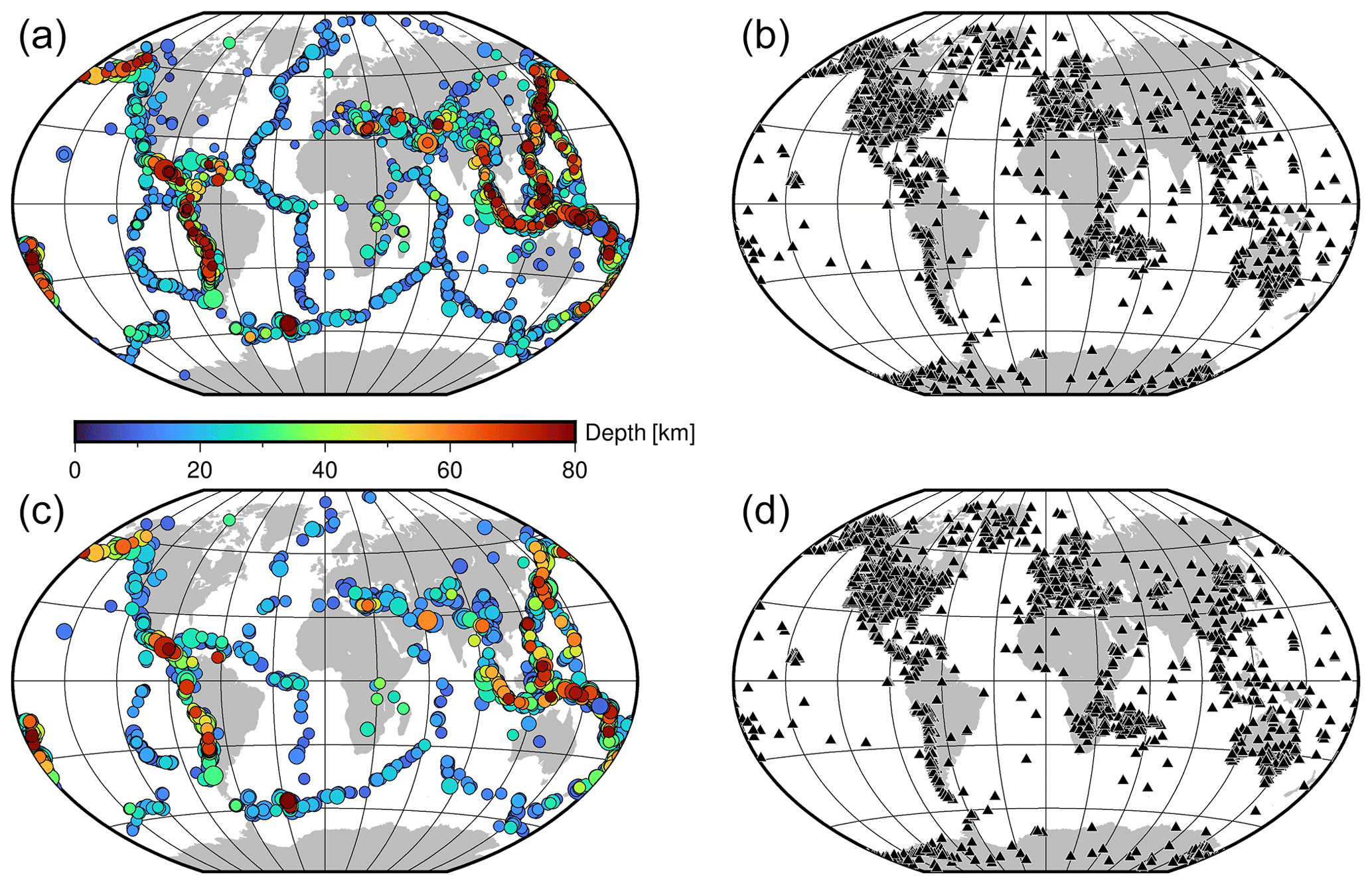
Figure 2Panels (a) and (b) show event and station locations for dataset D3 (Table 1), respectively. Panels (c) and (d) show event and station locations for dataset D6 (Table 1), respectively.
Table 1Datasets considered in this study. Datasets in bold are available in Bindi et al. (2024).
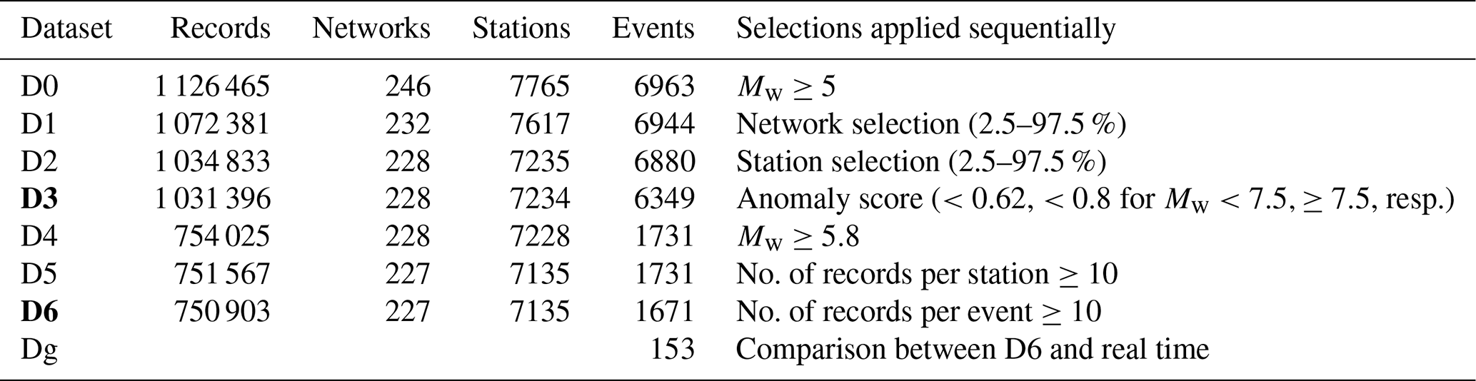
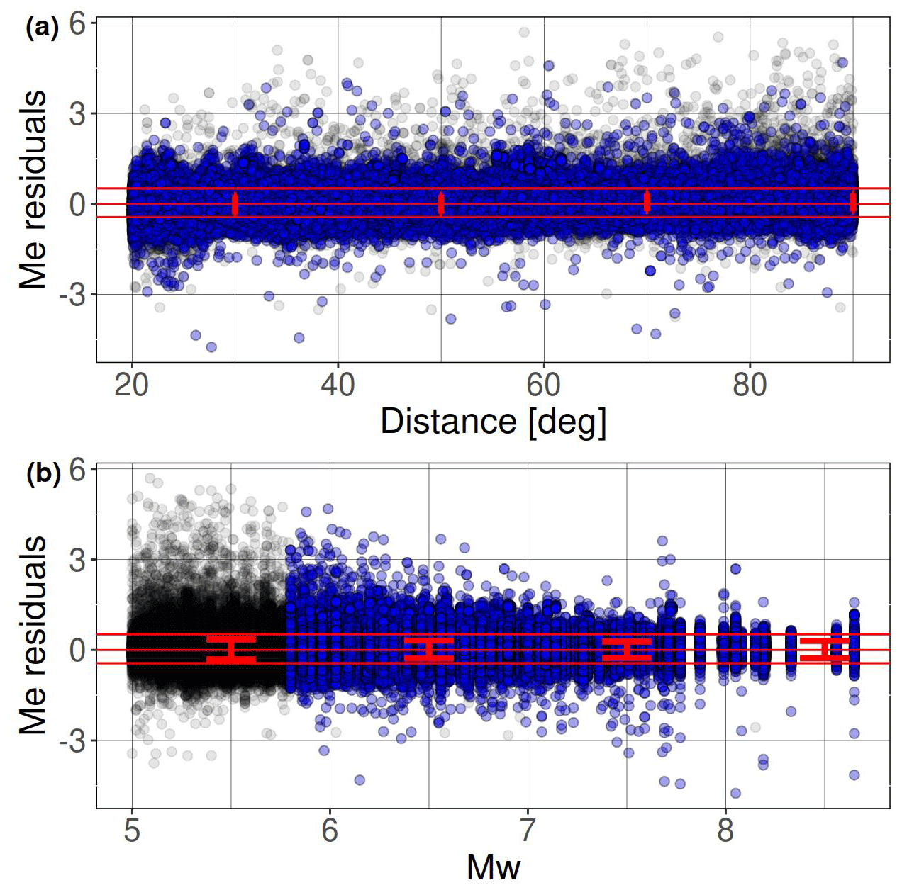
Figure 3Energy magnitude residuals versus distance (a) and moment magnitude (b) for dataset D3. Blue dots indicate residuals also included in D6. The horizontal red lines bound the 90 % confidence interval of the residual distribution. The error bars indicate the mean ±1 standard deviation of the residuals computed over different distance (20° wide) and magnitude (1 m.u. wide) intervals.
Therefore, we further limit the dataset by only considering events with Mw≥5.8 and at least 10 single-station measurements; we further exclude stations with fewer than 10 recordings in total. We added a column in the disseminated D3 dataset to flag lines corresponding to D6. It consists of ∼750 000 waveforms for 1671 earthquakes and 7135 stations. The event and station locations of D6 are shown in Fig. 2c and d.
We perform residual analysis to validate the D6 catalog. The relationship between Me and Mw is analyzed by performing the following mixed-effects regression (Bates et al., 2015; Stafford, 2014):
where Meij is the single-waveform energy magnitude estimate at station j for earthquake i, Mwi is the moment magnitude of earthquake i, intercept c1 and slope c2 parameters define the median model, and δSi and δEj are terms that capture station-specific and earthquake-specific adjustments, respectively. ϵij accounts for the leftover effects (i.e., residuals that are specific to a particular path/waveform). The random effects δS, δE, and ϵ are zero mean normal distributions by construction. In particular, δSj (inter-station residual) can represent site effects or instrumental gain corrections, with most of the latter probably removed by the outlier filtering stages described above. The interevent residual δEi is an event-specific deviation from the Me expected for a given Mw from the linear regression term. Finally, ϵij can be thought of as a noise term for individual measurements, which can be either related to path-specific heterogeneity in attenuation with respect to the 1-D reference model or the influence of ambient noise on the actual measurement.
The interevent and inter-station term distributions are shown in Fig. 4, which are described by standard deviations of τ=0.246 and ϕS=0.188 m.u., respectively; the standard deviation of the ϵ is ϕ0=0.232 m.u. When combining the interevent variability τ with the intra-event variability equal to , we obtain the total standard deviation , which represents the variability in the single-station Meij residuals with respect to the average Me computed per event. It is worth noting that the δSj values can be used as station corrections to compute the energy magnitude of new events. In this case, the inter-station contribution to the total variability is removed, and the expected variability in the Meij distribution is reduced to . Finally, the linear regression model is defined by the coefficients m.u. and . Considering the simplicity of the linear model in Eq. (2) and the large dataset analyzed, the uncertainty in the median model (sometimes referred to as σμ; Atik and Youngs, 2014) is very low, increasing from 0.007 for Mw=6 to 0.039 for Mw=9.
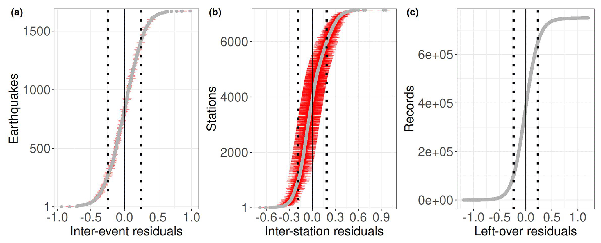
Figure 4Cumulative distribution functions for event δE (a), station δS (b), and leftover ϵ distributions (circles) determined according to the mixed-effects regression in Eq. (2) applied to dataset D6. Dotted lines correspond to standard deviations ±1τ (a), ±1ϕS (b), and ±1ϕ0 (c). Horizontal red lines in panels (a) and (b) are the standard errors in the random effects. In panel (c), values of ϵ exceeding ±1.2 in absolute value are not shown.
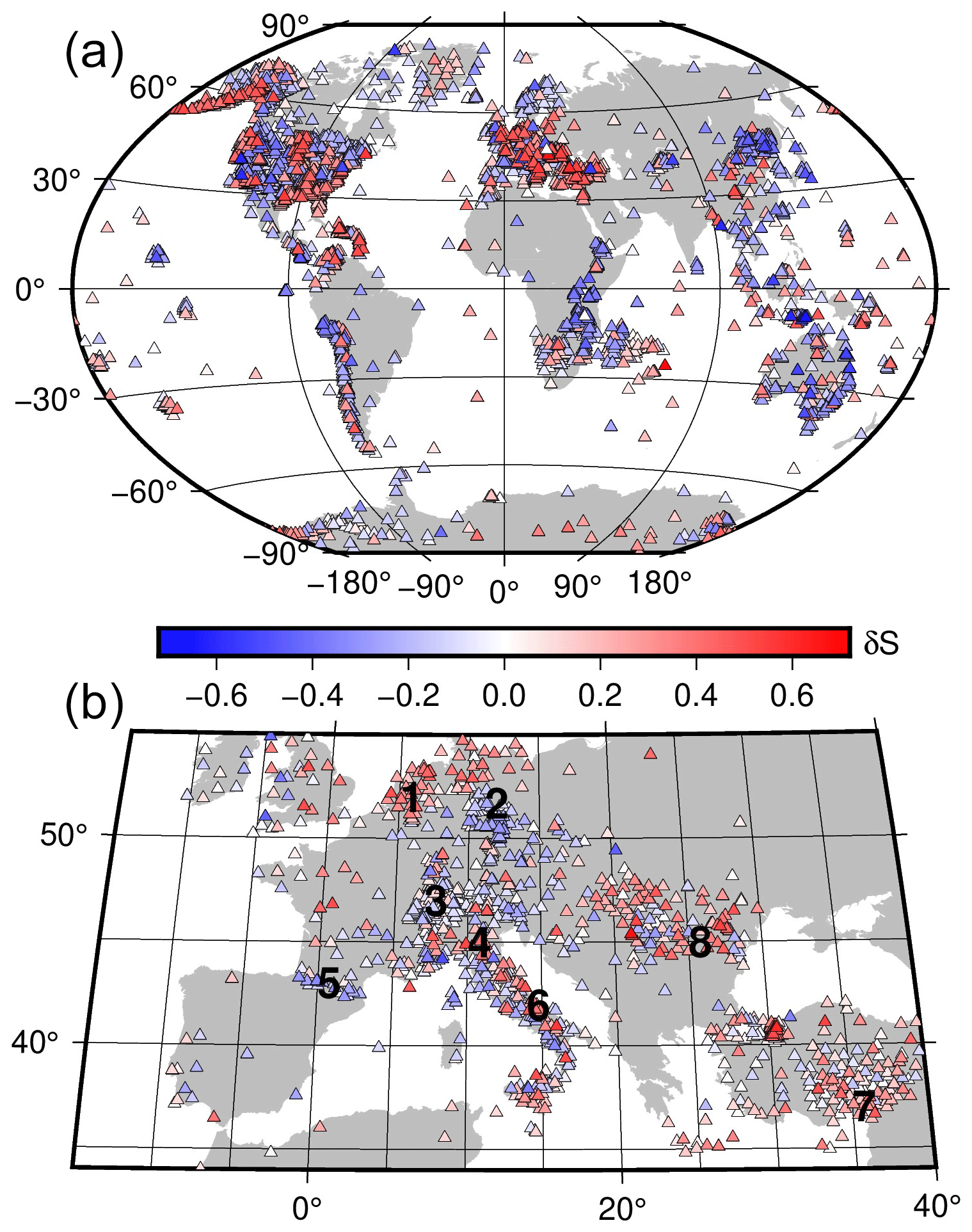
Figure 5(a) Distribution of the site-specific residuals δS (see Eq. 2) and (b) magnified view over a portion of Europe. Numbers in panel (b) indicate the following locations: (1) Netherlands; (2) Harz highlands, Germany; (3) Switzerland; (4) Po plain, Italy; (5) Pyrenees mountain range; (6) Apennine Mountains; (7) East Anatolian Fault region; and (8) Moesian Platform.
We show the spatial distribution of δS in Fig. 5. Since Meij is computed considering spectral values below 1 Hz and using teleseismic recordings for distances above 20°, δS capture station-specific effects connected to large-scale geological and tectonic crustal features, as exemplified in Fig. 5b for stations located in Europe. Positive δS (i.e., Meij larger than the median) are observed for stations located in basins like in the Po plain, in the Moesian region, in the Netherlands, and in the East Anatolian Fault region. Negative values δS (i.e., Meij lower than the median) are observed for stations located in mountain ranges such as the Pyrenees, the Alps, or in Harz Highlands and also tectonically highly active regions that are as cratonic as the East African Rift. The station terms can represent both site amplification, e.g., for stations in sedimentary basins, and anomalously high or low attenuation in the crust and or mantle surrounding the station. The station-specific residuals are disseminated along with the catalog to allow the computation of Me for future earthquakes, while taking into account static magnitude corrections to reduce variability.
The spatial distribution of the interevent variability, δE, is shown in Fig. 6 for the smallest and largest values.
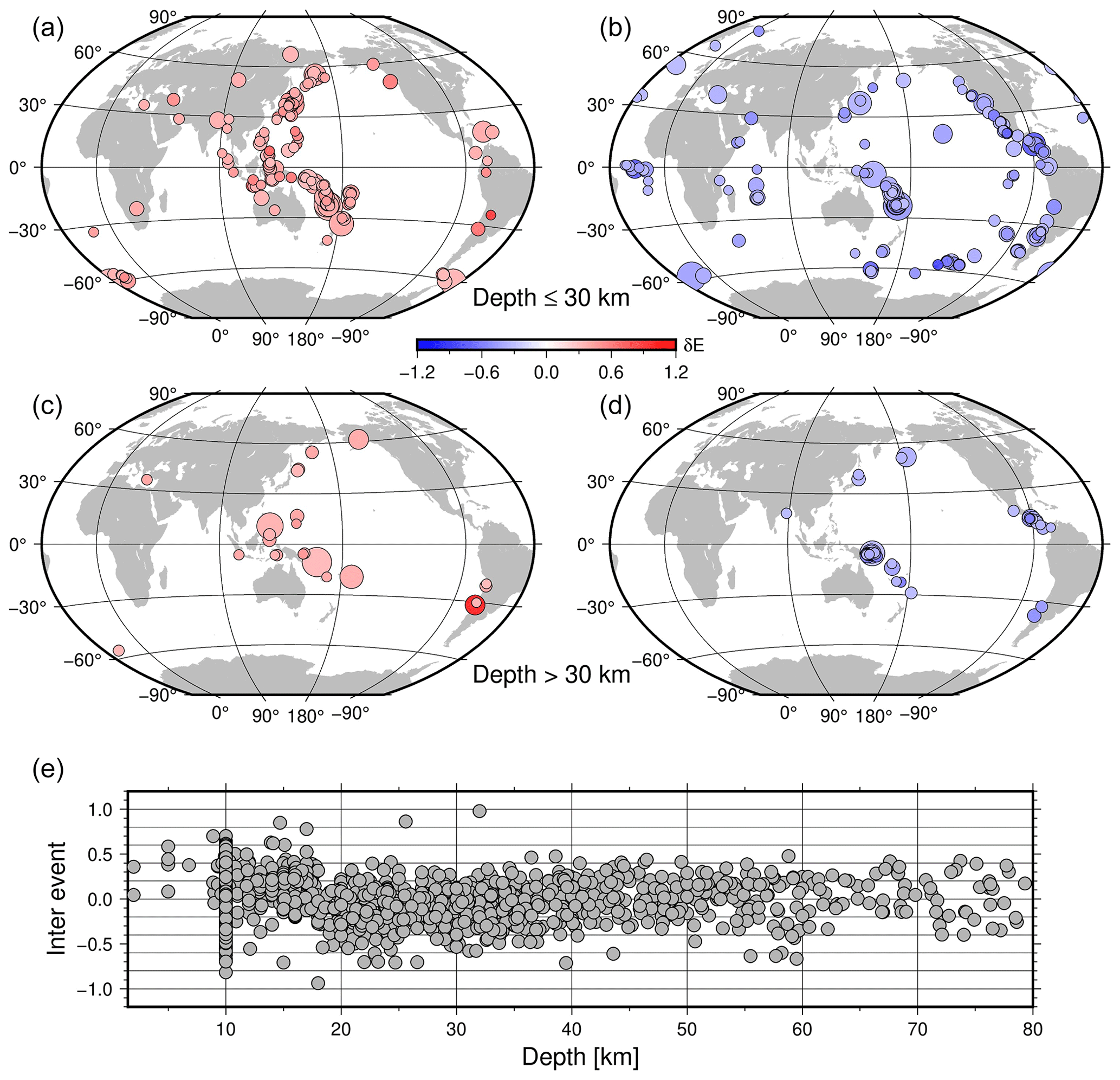
Figure 6Extreme values for event specific residuals δE for the Meij versus Mw mixed-effects model of Eq. (2). Only values below the 10th percentile (panels b and d) and above the 90th percentile (panels a and c) of the distribution are shown (the percentiles are about ±0.3). In panels (a) and (b), earthquakes with hypocentral depths shallower than 30 km are selected. In panels (c) and (d), events deeper than 30 km are considered. The distribution of δE versus depth for all events is shown in panel (e).
Considering depths shallower than 30 km (Fig. 6a and b), continental Asia, the Philippines, and Indonesia, as well as the Aleutian Islands, show positive values. California, Mexico, central America, and the Mid-Atlantic Ridge are characterized mostly by negative values. Considering deeper events (Fig. 6c and d), Japan and the Philippines have mostly positive values, while Mexico and central America have mostly negative values. The event-specific residuals are also disseminated, along with the catalog to increase the usefulness of the product from the event point of view, to allow the user to perform further refinements.
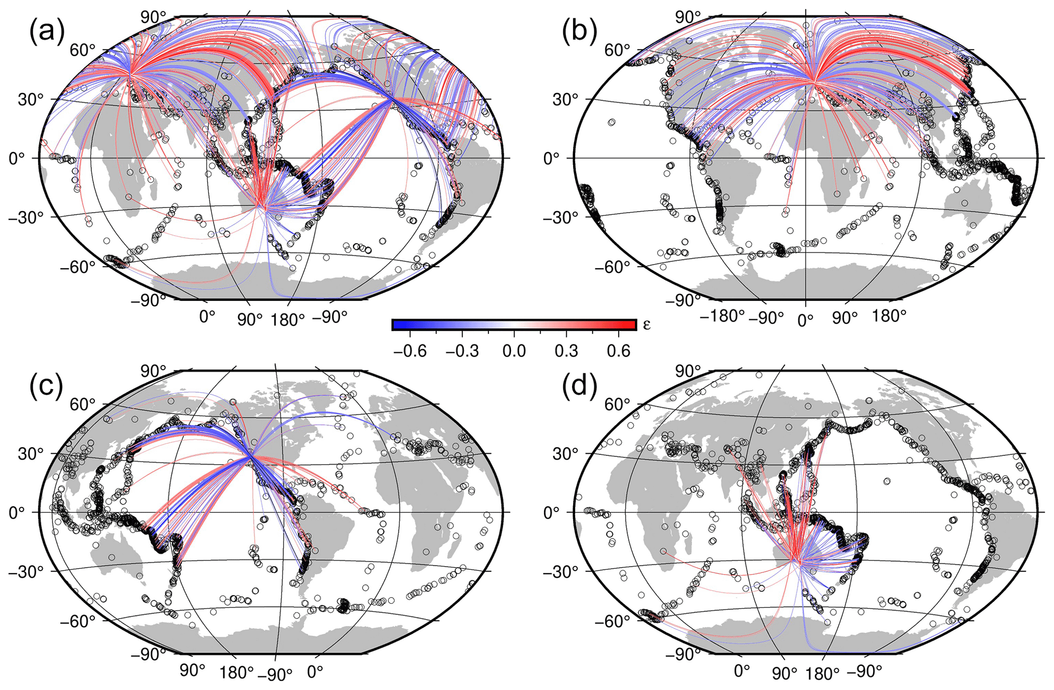
Figure 7(a) Residual distribution ϵ of Eq. (2) for three different receiving areas, showing only . (b) As in panel (a) but considering only the European receiving area. (c) As in panel (a) but considering only the receiving area in California. (d) As in panel (a) but considering only the receiving area in Australia. Circles indicate the earthquake locations.
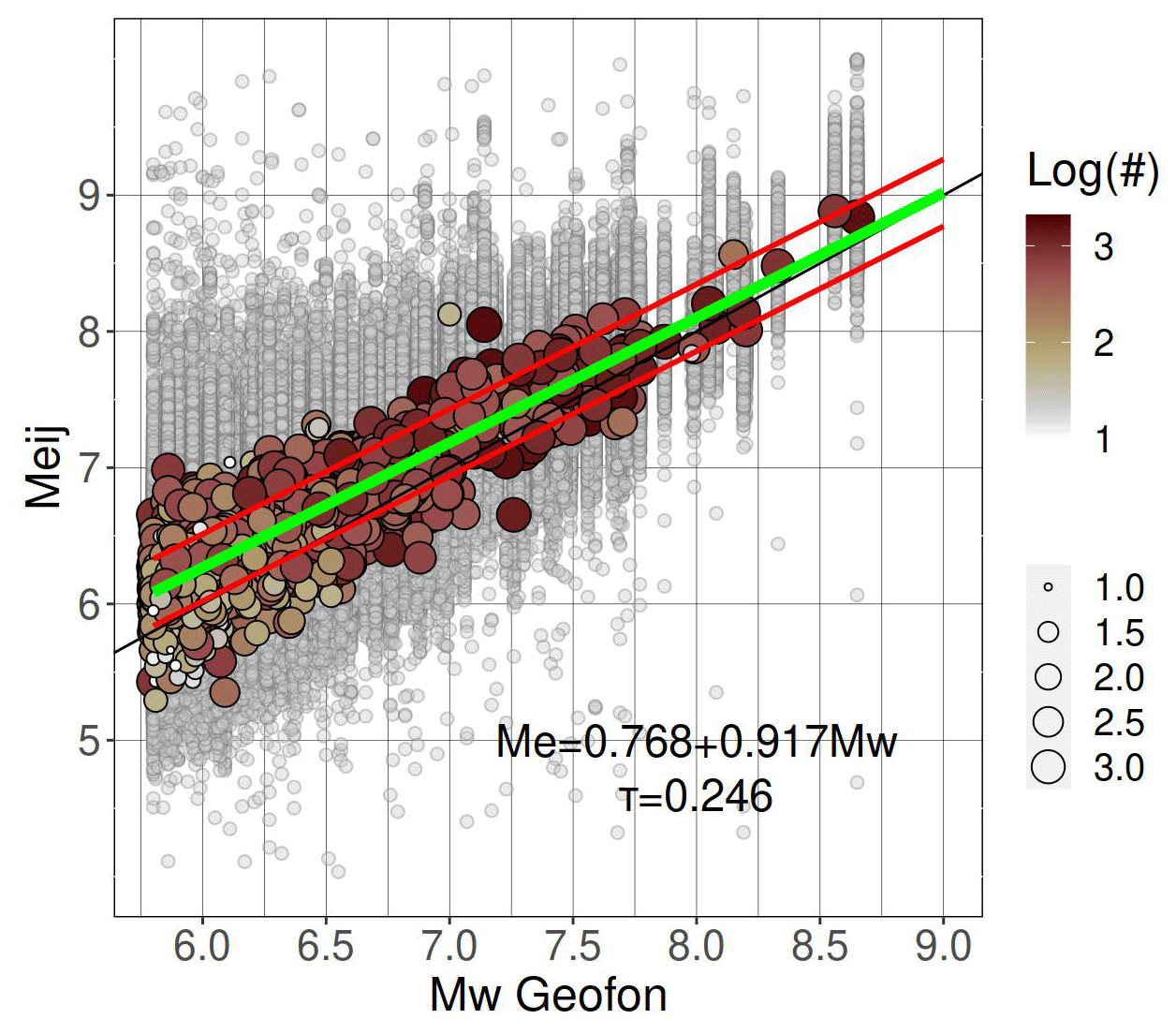
Figure 8Meij versus Mw scaling. Gray circles are the station Meij estimates, and filled circles represent event Me values calculated as medians of all station estimates for that event. Color indicates how many stations contributed to each estimate. The best-fit line in green is derived from the mixed-effects regression (Eq. 2), considering ±1 interevent standard deviation τ (red lines). The faint black line shows equality for reference.
Path-specific residuals ϵ are shown in Fig. 7 for three selected receiving areas in Europe, California, and Australia. Since in the partition of the residuals the leftover distribution ϵ represents the component not related to systematic station and event effects, they are mostly connected to lateral variability in attenuation in the Earth's interior with respect to the used global 1-D model and amplitude variation related to P-wave radiation patterns for different focal mechanisms.
Finally, the Meij versus Mw scaling defined by the linear regression coefficients c1 and c2 of Eq. (2) is shown in Fig. 8.
4.1 Catalog validation: comparison with IRIS
The energy magnitude computed in this study is compared to the values disseminated by IRIS through the SPUD service IRIS DMC (2013). The methodology implemented by IRIS is described by Convers and Newman (2011) and based on the analysis of Boatwright and Choy (1986) and Newman and Okal (1998). Similar to our approach, the energy flux is computed from the P-wave group (P + pP + sP) in the frequency domain. The single-station estimations are corrected for frequency-dependent anelastic attenuation effects and converted back to the energy radiated by the source by applying corrections for geometrical spreading, depth, and mechanism-dependent effects for P waves and considering a theoretical partition of the energy between P and S waves. The energy is computed considering the frequency range 0.014–2 Hz (broadband for Me(BB)) or 0.5-02 Hz (high frequency for Me(HF)), analyzing stations in the distance range 25–80°. The duration of the time window used for the computation is based on analysis of the cumulative high-frequency energy (0.5–2 Hz) as a function of time. The crossover time used to compute the energy flux is identified at the intersection between the near-constant increasing rate for short times and the relative flat asymptotic behavior for long durations. The SPUD service disseminates both the high-frequency Me(HF) and broadband Me(BB) estimates.
Two regression models are calibrated against the broadband and high-frequency estimates disseminated by IRIS through SPUD. The best-fit models, shown in Fig. 9, are and , with the standard deviation of the residuals equal to 0.234 and 0.175, respectively. For the magnitude range from 6 to 8, this results in biases of 0.06 m.u. for Me vs. Me(HF) and varying from 0.17 to −0.04 m.u. for Me vs. Me(BB); i.e., our estimates are nearly unbiased relative to Me(HF) and tend to slightly overestimate Me(BB) at the lower end of the applicability range.
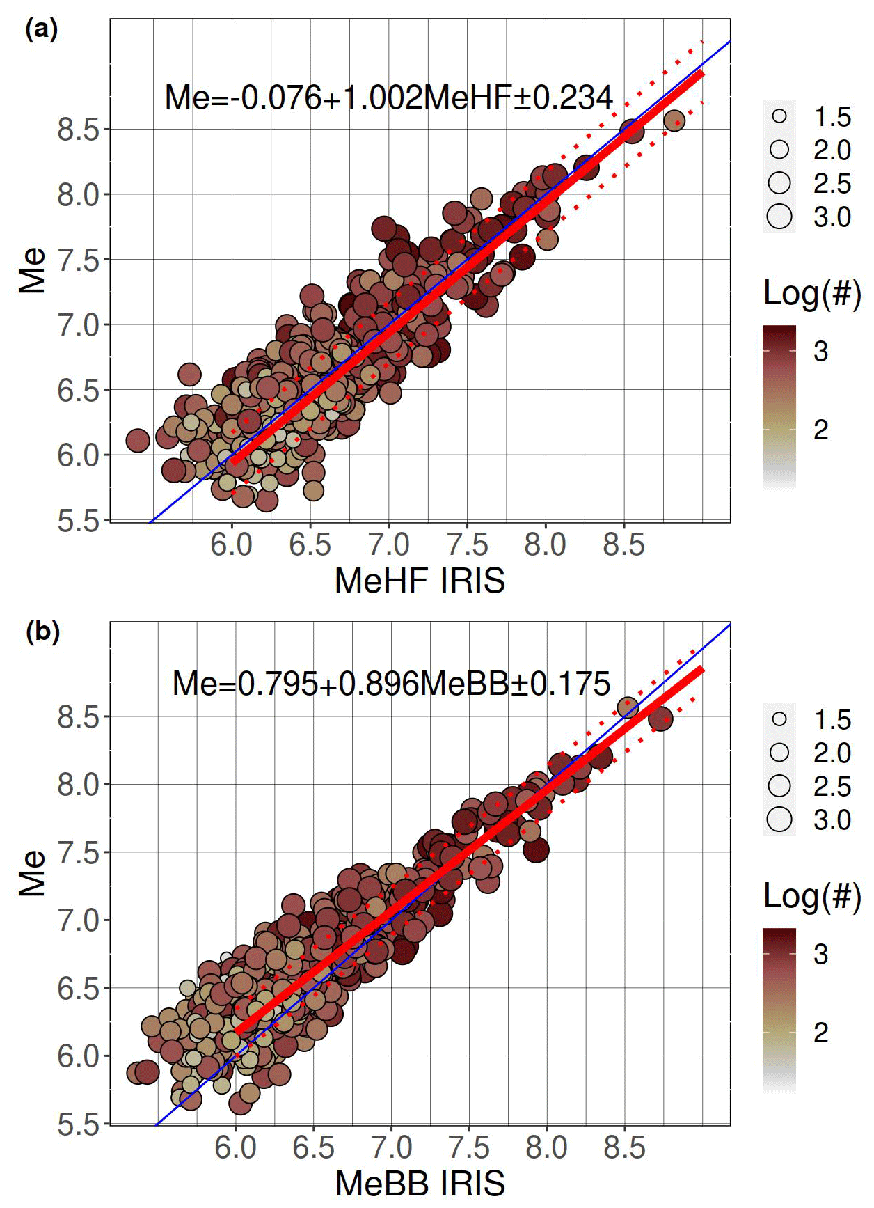
Figure 9Comparison with energy magnitude disseminated by IRIS considering (a) Me(HF) and (b) Me(BB) (717 common events). The red line shows the linear regression fit, and the dotted lines show 1 standard deviation of the Me residuals. The blue line shows line of equality for reference.
4.2 Catalog validation: role of style of faulting
The faulting style is classified into normal, reverse, and strike slip categories, based on the plunge of the P, T, and N axes (Frohlich and Apperson, 1992), as extracted from the GEOFON moment tensor solutions. There is a normal fault (NF) if the plunge (P) ≥60°, a strike slip (SS) if the plunge (N) ≥60°, and a thrust fault (TF) if the plunge T≥50°. In the other cases, the earthquake is labeled with OF (other faulting styles). To investigate the role of the style of faulting (SOF), we separate the event term into a fixed offset for each SOF class and a perturbation term for each event. If we indicate the classes of the SOF grouping factor (corresponding to NF, SS, TF, and OF) with and the class of event i with ki, then the equation for the extended mixed-effects model is
where δSOF are the terms characterizing the average effects of the different SOF and δESOF are accounting for interevent differences within each SOF class (nested random effects). The standard deviations of the δS, δSOF, δESOF, and ϵ distributions are ϕS=0.190, τSOF=0.095, τ=0.236, and ϕ0=0.232, respectively, generating a total standard deviation σ=0.393. The SOF terms are δSOF1=0.098 (NF), (SS), (TF), and δSOF4=0.055 (OF) (Fig. 10). The largest difference is between SS and NF, a total of 0.206 m.u. There is a systematic impact of the SOF on the intercept of the model, but the associated variability is smaller compared to the interevent variability τ (in other words, SOF effects are statistically significant, but the distributions of interevent terms separated according to faulting style are strongly overlapping).
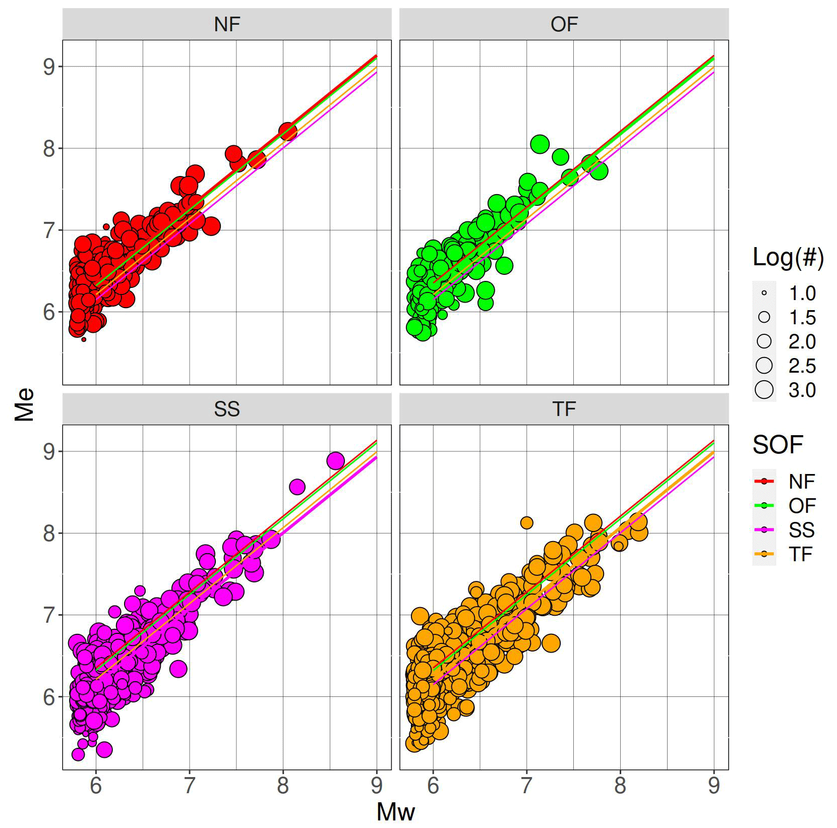
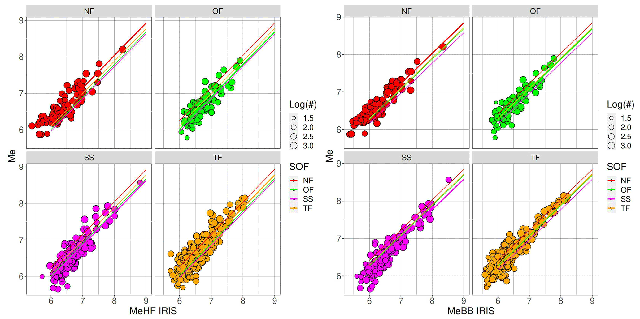
The SOF effects might arise due to physical differences (on average) between the different faulting types, e.g., due to systematically different stress drops, differences in the maturity of faults or typical environments (intra-plate vs. interplate), where different faulting types occur most often, or they might be artifacts due to the fact that the (Di Giacomo et al., 2008) method used here does not account for radiation pattern effects, and the teleseismic arrivals utilized here preferentially sample certain parts of the focal sphere. Therefore, we also investigate the role of the SOF in the relationship between Me derived in this study and the Me(HF) and Me(BB) values disseminated by IRIS. We recall that the methodology implemented by IRIS accounts for radiation pattern effects, which are related to the SOF. For this analysis, the regression model is the following:
where Miris is either Me(HF) or Me(BB). Results shown in Fig. 11 confirm that the largest intercept difference is between normal and strike slip events, and the differences in terms of magnitude units (m.u.) are also similar between the other SOF. This suggests that a large part of the SOF term is influenced by radiation pattern effects, and interpretations of these differences in terms of geodynamics or hazard potential should be done very cautiously.
The module, derived from me-compute has been integrated to the SeisComP package (Helmholtz Centre Potsdam GFZ German Research Centre for Geosciences and GEMPA GmbH, 2008) and has been part of the GEOFON routine real-time processing since December 2021. The first event for which Me calculations are available and disseminated via the usual GEOFON services is https://geofon.gfz-potsdam.de/eqinfo/event.php?id=gfz2021xxzt (last access: March 2024), which occurred on 7 December 2021 10:28:00.3 UTC (Me 5.7 and Mw 5.5). The scmert add-on is available at https://github.com/SeisComP/scmert (last access: March 2024).
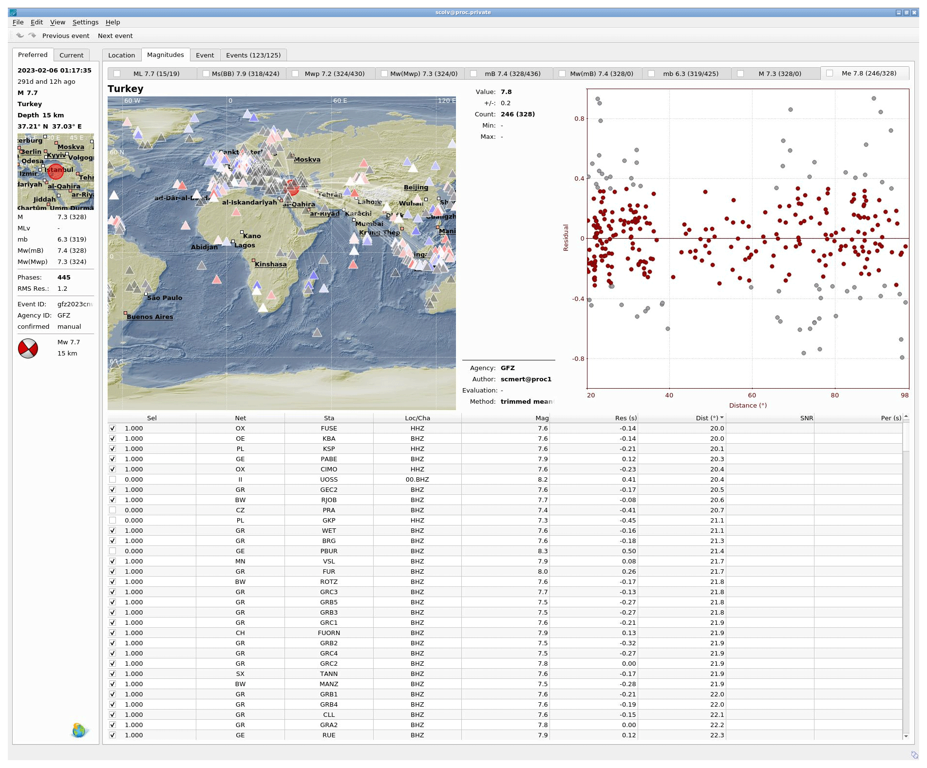
Figure 12Screenshot of the SeisComP Origin Locator View (scolv) interactive tool for the Mw 7.7 Republic of Türkiye earthquake that occurred on 6 February 2023, 01:17 UTC along the East Anatolian Fault. The obtained network magnitude value of Me is 7.8. Stations used are color-coded according to Me magnitude residuals (top-left frame). Stations in gray are excluded from the network magnitude, do not match the distance range definition, or were trimmed while computing the average magnitude because they are within the ±12.5 % range. The top-right scatterplot shows Me residuals by distance (in red those that contributed to actual Me network magnitude). The topography shown in the map is generated using the ETOPO1 global relief model (Amante and Eakins, 2009).
The add-on has been configured in GEOFON to trigger the calculation for each origin created by the automatic processing with magnitude ≥5.5 and to compute station magnitudes Meij for all stations according to the definition of Me in the distance 20–98°. The scmert procedure is applied with the settings used by the GEOFON Earthquake Information Service, using stations available in real time from the GEOFON Extended Virtual Network (https://geofon.gfz-potsdam.de/eqinfo/gevn/, last access: March 2024), including station selection and the distribution trimming of 25 %. The workflow for Me computations is as follows: as soon as an automatically detected event reaches the magnitude threshold, scmert is triggered and starts to compute Meij upon receiving data from stations beyond 20°. The process continues until the selected window length (determined by the actual preliminary magnitude) of the last station at 98° is acquired. The first estimate of the magnitude Me is released shortly after collecting 20 Meij estimates from individual station, usually within a few minutes of the earthquake's origin time. SeisComP modules continue to refine the estimate until no further updates are required (this includes manual release at later stages). The computed station magnitudes Meij are fully integrated also into the SeisComP Origin Locator View Graphical User Interface (scolv GUI; Fig. 12), with station magnitudes and residuals displayed in a dedicated energy magnitude tab.
The energy magnitude values from both modules are compared in Fig. 13. We used scmert with the same settings as the GEOFON earthquake monitoring service, including station selection and trimming of the distributions. The values are in good agreement, and the best-fit model is , with a standard deviation of 0.118. The average difference computed for magnitudes between 6 and 8 is −0.028.
All values for Me that have been calculated since the start of the routine processing with scmert can be accessed via the fdsnws-event web service running at GEOFON by specifying Me as the magnitude type (i.e., https://geofon.gfz-potsdam.de/fdsnws/event/1/query?starttime=2021-12-07&magnitudetype=Me&includeallmagnitudes=true&nodata=404, last access: March 2024). These values are also disseminated to other agencies (e.g., ISC and EMSC) via the usual downstream channels, including a real-time push service.
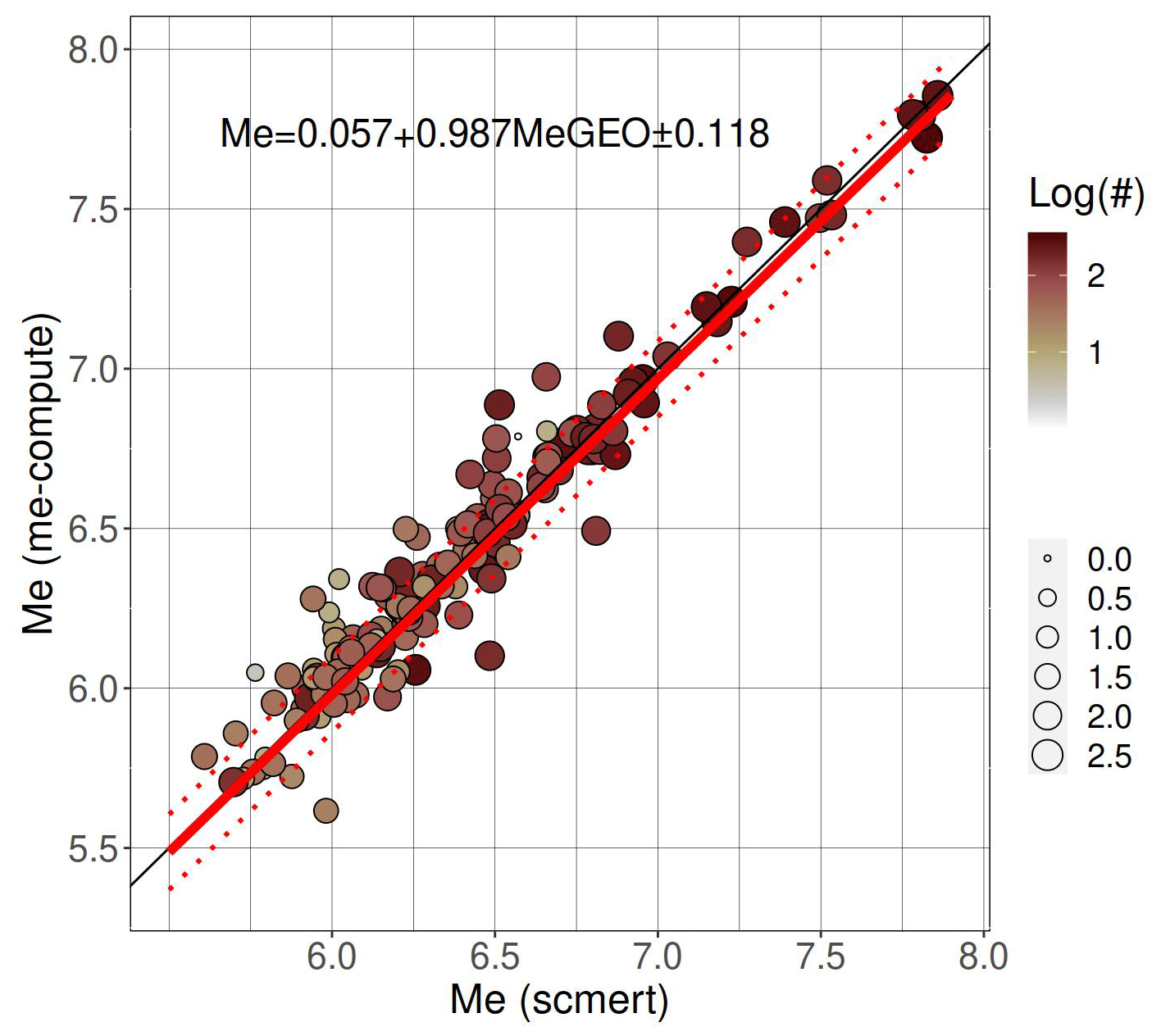
Figure 13Comparison between Me computed in real time by GEOFON, with the scmert add-on for SeisComP (x axis) and offline estimation using me-compute (y axis), considering 153 common events.
Code used for computing the energy magnitude is available from
-
offline computations in me-compute https://doi.org/10.5880/GFZ.2.6.2023.008 (Zaccarelli, 2023); and
-
real-time computations in SeisComP with scmert https://doi.org/10.5880/GFZ.2.4.2020.003 (Helmholtz Centre Potsdam GFZ German Research Centre for Geosciences and GEMPA GmbH, 2008).
Analyses have been performed in R (https://www.R-project.org/, R Core Team, 2020), and we used the Generic Mapping Tools (https://www.generic-mapping-tools.org/, last access: March 2024; Wessel et al., 2013) to produce Figs. 2, 5, 6, and 7. The archive, including the energy magnitude catalog (D3 and D6 in Table 1), the complete list of references for the seismic networks analyzed in this article with me-compute, and an example of the configuration files, is available from Bindi et al. (2024) (https://doi.org/10.5880/GFZ.2.6.2023.010).
We computed the energy magnitude Me for 6349 events in the moment magnitude catalog disseminated by GEOFON. When combined with Mw, Me allows a better characterization of the tsunami and shaking potential of an earthquake. The procedure used to compile the dataset, which includes 1 031 396 Me values for each recording station, is described in detail. Residuals are evaluated using a mixed-effects regression, which partitions the overall residuals into event-specific and station-specific contributions. These random effects are included in the distributed catalog, enabling the computation of Me for future events and using inter-station residuals as station corrections to reduce the uncertainty in Me. They also enable the assessment of energy magnitude adjustments for specific regions or faulting mechanisms, using interevent residuals and locating propagation anomalies with respect to the global model used to compute Green's functions using the leftover residuals. The methodology employed for computing Me (Di Giacomo et al., 2008) is suitable for the rapid assessment of Me (Di Giacomo et al., 2010). Therefore, it has been implemented as a module for SeisComP, allowing the automatic computation of Me in real time and keeping the Me catalog up to date.
DB, AS, and DDG conceptualized the study. RZ developed the Python code used to compile the disseminated catalog. AH developed the add-on for SeisComP. DB developed the quality checks. PE, AH, and AS organized the publication of Me by GEOFON via web services. All authors participated to the finalization of the article.
The contact author has declared that none of the authors has any competing interests.
Publisher’s note: Copernicus Publications remains neutral with regard to jurisdictional claims made in the text, published maps, institutional affiliations, or any other geographical representation in this paper. While Copernicus Publications makes every effort to include appropriate place names, the final responsibility lies with the authors.
We thank all network operators providing data via EIDA–ORFEUS and IRIS, as well as all real-time data providers contributing to the GEOFON virtual network. We thank Kirsten Elger for her help in preparing the dissemination of the products of this study. Finally, we appreciated the valuable feedback and suggestions provided by two anonymous reviewers and by the editor Andrea Rovida.
he article processing charges for this open-access publication were covered by the Helmholtz Centre Potsdam – GFZ German Research Centre for Geosciences through the finacial support of the Horizon Europe project Geo-INQUIRE, funded by the European Commission (HORIZON-INFRA-2021-SERV-01, project no. 101058518).
The article processing charges for this open-access publication were covered by the Helmholtz Centre Potsdam – GFZ German Research Centre for Geosciences.
This paper was edited by Andrea Rovida and reviewed by two anonymous referees.
Aki, K.: Generation and Propagation of G Waves from the Niigata Earthquake of June 16, 1964. Part 2. Estimation of earthquake moment, released energy, and stress-strain drop from the G wave spectrum, B. Earthq. Res. I. Tokyo, 44, 73–88, https://doi.org/10.15083/0000033586, 1966. a
Amante, C. and Eakins, B. W.: ETOPO1 1 Arc-Minute Global Relief Model: Procedures, Data Sources and Analysis, NOAA Technical Memorandum NESDIS NGDC-24. National Geophysical Data Center, NOAA [data set], https://repository.library.noaa.gov/view/noaa/1163 (last access: March 2024), 2009. a
Atik, L. A. and Youngs, R. R.: Epistemic Uncertainty for NGA-West2 Models, Earthq. Spectra, 30, 1301–1318, https://doi.org/10.1193/062813EQS173M, 2014. a
Bates, D., Mächler, M., Bolker, B., and Walker, S.: Fitting Linear Mixed-Effects Models Using lme4, J. Stat. Softw., 67, 1–48, https://doi.org/10.18637/jss.v067.i01, 2015. a
Bindi, D,. Zaccarelli, R., Strollo, A., Di Giacomo, D., Heinloo, A., Evans, P., Cotton, F., and Tilmann, F.: Global energy magnitude catalog 2011–2023 with event selection driven by Mw Geofon, V. 1.1. GFZ Data Services [data set], https://doi.org/10.5880/GFZ.2.6.2023.010, 2024. a, b, c, d, e
Boatwright, J. and Choy, G. L.: Teleseismic estimates of the energy radiated by shallow earthquakes, J. Geophys. Res.-Sol. Ea., 91, 2095–2112, https://doi.org/10.1029/JB091iB02p02095, 1986. a, b
Bormann, P., Baumbach, M., Bock, G., Grosser, H., Choy, G., and Boatwright, J.: Seismic Sources and Source Parameters, in: IASPEI New Manual of Seismological Observatory Practice, edited by Bormann, P., vol. 1, chap. 3, 94 pp., Deutsches GeoForschungsZentrum GFZ, Potsdam, https://gfzpublic.gfz-potsdam.de/pubman/item/item_4015 (last access: March 2024), 2002. a
Convers, J. A. and Newman, A. V.: Global Evaluation of Large Earthquake Energy from 1997 Through mid-2010, J. Geophys. Res., 116, B08304, https://doi.org/10.1029/2010JB007928, 2011. a
Di Giacomo, D., Grosser, H., Parolai, S., Bormann, P., and Wang, R.: Rapid determination of Me for strong to great shallow earthquakes, Geophys. Res. Lett., 35, L10308, https://doi.org/10.1029/2008GL033505, 2008. a, b, c, d, e, f
Di Giacomo, D., Parolai, S., Bormann, P., Grosser, H., Saul, J., Wang, R., and Zschau, J.: Suitability of rapid energy magnitude determinations for emergency response purposes, Geophys. J. Int., 180, 361–374, https://doi.org/10.1111/j.1365-246X.2009.04416.x, 2010. a, b, c, d, e
Di Giacomo, D., Harris, J., and Storchak, D. A.: Complementing regional moment magnitudes to GCMT: a perspective from the rebuilt International Seismological Centre Bulletin, Earth Syst. Sci. Data, 13, 1957–1985, https://doi.org/10.5194/essd-13-1957-2021, 2021. a
Frohlich, C. and Apperson, K. D.: Earthquake focal mechanisms, moment tensors, and the consistency of seismic activity near plate boundaries, Tectonics, 11, 279–296, https://doi.org/10.1029/91TC02888, 1992. a
Gutenberg, B.: Amplitudes of surface waves and magnitudes of shallow earthquakes, B. Seismol. Soc. Am., 35, 3–12, 1945a. a
Gutenberg, B.: Amplitudes of P, PP, and S and magnitude of shallow earthquakes, B. Seismol. Soc. Am., 35, 57–69, https://doi.org/10.1785/BSSA0350020057, 1945b. a
Hanks, T. C. and Kanamori, H.: A moment magnitude scale, J. Geophys. Res., 84, 2348–2350, https://doi.org/10.1029/JB084IB05P02348, 1979. a
Haskell, N. A.: Total energy and energy spectral density of elastic wave radiation from propagating faults, B. Seismol. Soc. Am., 54, 1811–1841, https://doi.org/10.1785/bssa05406a1811, 1964. a, b
Helmholtz Centre Potsdam GFZ German Research Centre for Geosciences and GEMPA GmbH: The SeisComP seismological software package, GFZ Data Services [code], https://doi.org/10.5880/GFZ.2.4.2020.003, 2008. a, b
IRIS DMC: Data Services Products: EQEnergy Earthquake energy & rupture duration, https://doi.org/10.17611/DP/EQE.1, 2013. a
Kanamori, H.: The energy release in great earthquakes, J. Geophys. Res., 82, 2981–2987, https://doi.org/10.1029/JB082I020P02981, 1977. a
Kennett, B. L. N., Engdahl, E. R., and Buland, R.: Constraints on seismic velocities in the Earth from traveltimes, Geophys. J. Int., 122, 108–124, https://doi.org/10.1111/j.1365-246x.1995.tb03540.x, 1995. a
Montagner, J.-P. and Kennett, B.: How to reconcile body-wave and normal-mode reference Earth models?, Geophys. J. Int., 125, 229–248, 1996. a
Newman, A. V. and Okal, E. A.: Teleseismic estimates of radiated seismic energy: The discriminant for tsunami earthquakes, J. Geophys. Res.-Sol. Ea., 103, 26885–26898, https://doi.org/10.1029/98JB02236, 1998. a, b
Quinteros, J., Strollo, A., Evans, P. L., Hanka, W., Heinloo, A., Hemmleb, S., Hillmann, L., Jaeckel, K., Kind, R., Saul, J., Zieke, T., and Tilmann, F.: The GEOFON Program in 2020, Seismol. Res. Lett., 92, 1610–1622, https://doi.org/10.1785/0220200415, 2021. a
R Core Team: R: A Language and Environment for Statistical Computing, R Foundation for Statistical Computing, Vienna, Austria, https://www.R-project.org/ (last access: March 2024), 2020. a
Stafford, P. J.: Crossed and Nested Mixed‐Effects Approaches for Enhanced Model Development and Removal of the Ergodic Assumption in Empirical Ground‐Motion Models, B. Seismol. Soc. Am., 104, 702–719, https://doi.org/10.1785/0120130145, 2014. a
Strollo, A., Cambaz, D., Clinton, J., Danecek, P., Evangelidis, C. P., Marmureanu, A., Ottemöller, L., Pedersen, H., Sleeman, R., Stammler, K., Armbruster, D., Bienkowski, J., Boukouras, K., Evans, P. L., Fares, M., Neagoe, C., Heimers, S., Heinloo, A., Hoffmann, M., Kaestli, P., Lauciani, V., Michalek, J., Odon Muhire, E., Ozer, M., Palangeanu, L., Pardo, C., Quinteros, J., Quintiliani, M., Antonio Jara‐Salvador, J., Schaeffer, J., Schloemer, A., and Triantafyllis, N.: EIDA: The European Integrated Data Archive and Service Infrastructure within ORFEUS, Seismol. Res. Lett., 92, 1788–1795, https://doi.org/10.1785/0220200413, 2021. a
Wang, R.: A simple orthonormalization method for stable and efficient computation of Green’s functions, B. Seismol. Soc. Am., 89, 733–741, https://doi.org/10.1785/BSSA0890030733, 1999. a
Wessel, P., Smith, W. H. F., Scharroo, R., Luis, J., and Wobbe, F.: Generic Mapping Tools: Improved Version Released, Eos, 94, 409–410, https://doi.org/10.1002/2013EO450001, 2013. a
Zaccarelli, R.: Stream2segment: a tool to download, process and visualize event-based seismic waveform data (Version 2.7.3), GFZ Data Services [code], https://doi.org/10.5880/GFZ.2.4.2019.002, 2018. a
Zaccarelli, R.: sdaas – a Python tool computing an amplitude anomaly score of seismic data and metadata using simple machine‐Learning models, GFZ Data Services [code], https://doi.org/10.5880/GFZ.2.6.2023.009, 2022. a
Zaccarelli, R.: me-compute: a Python software to download events and data from FDSN web services and compute their energy magnitude (Me), GFZ Data Services [code], https://doi.org/10.5880/GFZ.2.6.2023.008, 2023. a, b
Zaccarelli, R., Bindi, D., Strollo, A., Quinteros, J., and Cotton, F.: Stream2segment: An Open‐Source Tool for Downloading, Processing, and Visualizing Massive Event‐Based Seismic Waveform Datasets, Seismol. Res. Lett., 90, 2028–2038, https://doi.org/10.1785/0220180314, 2019. a
Zaccarelli, R., Bindi, D., and Strollo, A.: Anomaly Detection in Seismic Data – Metadata Using Simple Machine‐Learning Models, Seismol. Res. Lett., 92, 2627–2639, https://doi.org/10.1785/0220200339, 2021. a
- Abstract
- Introduction
- Energy magnitude computation
- Catalog compilation
- Quality assessment via residual analysis
- Real-time module for SeisComP
- Code and data availability
- Conclusive remarks
- Author contributions
- Competing interests
- Disclaimer
- Acknowledgements
- Financial support
- Review statement
- References