the Creative Commons Attribution 4.0 License.
the Creative Commons Attribution 4.0 License.
 | 20 Mar 2024
FOCA: a new quality-controlled database of floods and catchment descriptors in Italy
Pierluigi Claps
Giulia Evangelista
Daniele Ganora
Paola Mazzoglio
Irene Monforte
Here we present FOCA (Italian FlOod and Catchment Atlas), the first systematic collection of data on Italian river catchments for which historical discharge time series are available. Hydrometric information, including the annual maximum peak discharge and average daily annual maximum discharge, is complemented by several geomorphological, climatological, extreme rainfall, land-cover and soil-related catchment attributes. All hydrological information derives from the most recently released datasets of discharge and rainfall measurements. To enhance the reproducibility and transferability of the analysis, this paper provides a description of all the raw data and the algorithms used to build the basin attribute dataset. We also describe the approaches adopted to solve problems encountered during the digital elevation model elaboration in areas characterized by a complex morphology. Details about the data quality-control procedure developed to detect and correct errors are also reported. One of the main novelties of FOCA with respect to other national-scale datasets is the inclusion of a rich set of geomorphological attributes and extreme rainfall features for a large set of basins covering a wide range of elevations and areas. Using this first nationwide data collection (available at https://doi.org/10.5281/zenodo.10446258, Claps et al., 2023), a wide range of environmental applications, with a particular focus on flood studies, can be undertaken within the Italian territory.
- Article
(7393 KB) - Full-text XML
- BibTeX
- EndNote


The availability of complete, updated and quality-controlled hydro-geomorphological information for areas nationwide is a key requirement for a vast range of applications from hydrological modeling to hydraulic simulations and rainfall–runoff analyses. Hydro-geomorphological catchment information, also called catchment attributes, can also provide a comprehensive description of the landscape and of how the catchment stores and transfers water (Addor et al., 2017).
The work of Linke et al. (2019), who created the HydroATLAS database by mapping key hydrological variables at 500 m grid resolution, represents a considerable effort to provide hydrological, climatological and land-cover information on a global scale. In that work, however, few hydrological and climatic attributes were considered, and geomorphological catchment descriptors are completely missing from it. In Europe, the importance of river basin catalogs acting as a support to water resources management was strongly stressed by the publication of the Water Framework Directive in 2000. River catchments that cross administrative boundaries can suffer from a lack of incomplete and non-uniform information. To tackle this shortcoming, in early 2000, an initiative undertook the creation of a pan-European river and catchment database (Vogt et al., 2007). In recent years, considerable efforts have been dedicated to producing similar datasets at the national scale for several European countries. Relevant examples are the datasets built in the framework of the CAMELS (Catchment Attributes and MEteorology for Large-sample Studies) initiative, as in the cases of Great Britain (Coxon et al., 2020), France (Andréassian et al., 2021; Delaigue et al., 2022), Switzerland (Höge et al., 2023) and Germany (Loritz et al., 2022). Similar datasets from other continents that were developed within the same framework have also been released, such as those for the United States (Addor et al., 2017), Chile (Alvarez-Garreton et al., 2018), Brazil (Chagas et al., 2020) and Australia (Fowler et al., 2021). Most of those datasets have since been linked together in order to build the Caravan dataset (Kratzert et al., 2023). Previous notable examples are the atlases and datasets developed in Switzerland (https://hydrologicalatlas.ch/, last access: 11 March 2024), Austria (Fürst et al., 2009) and Canada (Arsenault et al., 2016). In recent years, other large-scale datasets have been developed independently of the CAMELS framework, such as those related to China (Hao et al., 2021) and to the area of the upper Danube up to the Austria–Slovakia border and some nearby catchments (Klingler et al., 2021).
As of today, only partial-coverage datasets (in terms of both spatial extent and the number of variables) are available for Italy. We can mention the datasets developed for the northwest of Italy (see, e.g., Barbero et al., 2012; Gallo et al., 2013), the northeast of Italy (Crespi et al., 2021) and North-Central Italy (Pavan et al., 2019) as well as some studies that aimed at mapping a few variables across the entirety of Italy (ISPRA, 2005a, b; Claps et al., 2008; Crespi et al., 2018; Braca et al., 2021). Among the above examples, the database realized within the CUBIST (Characterisation of Ungauged Basins by Integrated uSe of hydrological Techniques) project (Claps et al., 2008) was the only attempt to build a multi-variable national data collection; all the other collections focus on only one specific topic (rainfall or discharge or geomorphology). A complete and updated database of hydro-geomorphological variables relating to the main catchments of Italy is therefore still missing. One of the reasons behind this gap is the dismantlement of the National Mareographic and Hydrographic Service (Servizio Mareografico e Idrografico Nazionale, SIMN), which has led to the federated management of the national monitoring network by 21 different administrative agencies. Nonetheless, the high network density of the rain and stream gauges that are available throughout the country allows the compilation of nationwide catalogs, which can also take advantage of the considerable number of local studies performed using systematic samples of hydrological measurements.
A recent effort to collect relevant hydrological information with national coverage is represented by the work of Claps et al. (2020a, b, c), in which annual maximum peak discharges (hereafter named “peak discharges” for brevity) and average daily annual maximum discharges (hereafter named “daily discharges” for brevity) from 1911 to 2016 for 631 Italian catchments are published, together with some basic geomorphological catchment attributes. This collection was mainly created to integrate previously untracked flood discharge measurements whose historical records were not available in hydrological yearbooks; they were only available in special publications. In this paper, we aim to substantially enhance the existing catchment and peak discharge catalogs by complementing the hydrological data with a large set of climatological, geomorphological, soil and land-use attributes, many of them computed from recently released databases. All data sources used comply with the following criteria: (a) nationwide coverage; (b) consistency in data quality (i.e., no regional or local biases); and (c) adequate original resolution in relation to the type of information. All the data sources used in this work can be downloaded from public repositories, except for a few variables that are not easily accessible. In these cases, the original data sources were included in the dataset created in this work, together with the mean catchment descriptors, to allow replicability. The result of this work is FOCA (Italian FlOod and Catchment Atlas), the first national-scale catchment attribute dataset in Italy (Claps et al., 2023).
The paper is structured as follows. In Sect. 2, the database history and the rationale used to select catchments to include in the database are described. In Sects. 3 and 4, we present the different categories of raw data (which were already partly quality-controlled and only required some adjustments), which largely relate to digital elevation models and streamflow measures, and partly processed data, which derive from the aggregation and manipulation of rainfall and soil information. In Sects. 3 and 4, we also provide an overview of all the geomorphoclimatic attributes computed for each catchment (together with the methodologies used for their definition and the algorithms used for their evaluation) to grant replicability and thus allow researchers to perform the same study or extend this one to other catchments. In Sect. 5 the data availability is presented. In Sect. 6, the main characteristics of the FOCA dataset are summarized, and some concluding remarks are presented.
Since the early 1990s, the Italian monitoring network was managed by the SIMN. This institution was in charge of the collection and validation of the data and its publication in a series of hydrological yearbooks with yearly updates. Two standardized documents (part I and part II) were usually published each year. The first volume (part I) was dedicated to temperature and precipitation; the second volume contained information and elaborations related to daily and monthly average discharges.
Due to this separation, to retrieve an entire time series measured by a gauging station, it was necessary to consult all the yearbooks. All the mentioned yearbooks are available as images (in gif format) at http://www.bio.isprambiente.it/annalipdf/ (last access: 23 October 2023). To facilitate access to the discharge data, this information was then processed by the SIMN at monthly time resolution and grouped by individual gauging station with the aim of providing several years of data on one data sheet for each station. This summarized information, available up to 1970 and complemented with some basic catchment information, became Pubblicazione no. 17 (Publication no. 17); this also included the annual peak values that were not directly available in the yearbooks. This document was updated about every 10 years from 1934 on (several issues are still available) by progressively including the data acquired up to 1970 (Servizio Idrografico, 1980).
Unfortunately, the updating of this publication was interrupted, as the SIMN was dismantled about 30 years ago and 21 different local agencies then became responsible for the management of the hydrographic services. This interruption of the publication of Pubblicazione no. 17 had a particularly negative effect on access to the peak discharge data. They were only published in Pubblicazione no. 17 as the maxima of the instantaneous discharge and have never been available in the hydrological yearbooks. This means that, for many years, peak discharges measured after 1970 were only available in the regional hydrographic offices. The main effort to recover these unpublished data was made by the GNDCI (Gruppo Nazionale per la Difesa dalle Catastrofi Idrogeologiche) as part of the VAPI (VAlutazione delle PIene) project (http://www.idrologia.polito.it/gndci/Vapi.htm, last access: 23 October 2023), which was subsequently integrated into the CUBIST project.
The first major advancement in the creation of a nationwide database was achieved by the CUBIST project (Claps et al., 2008). More specifically, historical information previously available only in printed format was digitized and merged with more recent data. Moreover, each catchment closed by the gauging stations included in this collection was characterized from a climatological and geomorphological point of view by means of the computation of key catchment attributes.
In the following years, some regional-scale works were conducted to update this systematic collection but without nationwide coordination. For example, in Northwest Italy, the first follow-up work was the Catalogo delle portate massime annuali al colmo del bacino occidentale del Po (Barbero et al., 2012), which includes a considerable number of additional observations from the gauging stations operated by the regional environmental agency as well as additional gauging stations managed by other public or private bodies, such as Enel (a major Italian energy provider) and the CNR (Italian Research Council). In this publication, a systematic and extensive data validation was performed to convert into discharge values the hydrometric stage values that had been recorded by the SIMN but had never been processed with adequate rating curves. This collection summarizes the information for 140 catchments with at least 5 years of data on peak or daily discharges, and it contains some basic information on the catchments. Unfortunately, this publication does not contain all the attributes evaluated within the CUBIST project. This regional collection was thus improved with the release of the Atlante dei bacini imbriferi piemontesi (Gallo et al., 2013), which contains geomorphological attributes of about 200 gauged river catchments located in the same region. In this case, however, the peak discharges were not reported, as they were not available for all the basins. Similar works were also carried out for other limited areas in the framework of local studies on flood frequency analysis (e.g., Rossi and Caporali, 2010).
Such collections of flood datasets were recently homogenized, integrated and updated by including the most recent data acquired across Italy, leading to the release of a comprehensive catalog of floods (Catalogo delle Piene dei Corsi d'acqua Italiani; Claps et al., 2020a, b, c). However, in this case, only basic geomorphological information was included for the considered basins.
The catchment selection criterion adopted in the present work stems from the purpose of improving upon the work reported in Claps et al. (2020a, b, c). The 631 chosen catchments are those for which peak or daily discharges are available and are therefore all included in Claps et al. (2020a, b, c). Details on the different sources of the historical discharge time series used and their integration are given in Sect. 4.4.
3.1 The digital elevation model
As of today, the only national-scale high-resolution digital elevation model (DEM) available for the whole of Italy is TINITALY/01 (Tarquini et al., 2007). Despite its very high spatial resolution (10 m) – which makes its use quite interesting, especially for the delineation of small catchments – it presents the drawback of being obtained by merging separate DEMs of single administrative regions, so it does not allow us to work with the same accuracy level nationwide. To overcome this drawback, we adopted the DEM from the Shuttle Radar Topography Mission (SRTM) at 30 m spatial resolution (Farr et al., 2007).
The processing of the DEM and, in general, all the other catchment attributes was performed with open-source software, namely GRASS GIS and R. In this work, the original SRTM DEM was re-projected into the WGS84/UTM zone 32N coordinate system by means of a bicubic interpolation and resampled to obtain integer cells, i.e., the data format requested by the GRASS GIS add-on r.basin (Di Leo and Di Stefano, 2013) that was used to derive most of the geomorphological attributes, as will be discussed in the following subsections. DEMs usually contains pits (i.e., elevation values that are much lower than those of nearby pixels; these are errors due to the resolution of the data) that should be filled to ensure the proper delineation of catchment boundaries and drainage networks. Thus, the pit-filling procedure was carried out using the r.hydrodem add-on for the GRASS GIS (Lindsay and Creed, 2005).
The r.basin add-on algorithm requires a series of information before it can be executed. The input parameters required by r.basin for the attribute extraction routine are presented in the following subsections.
3.2 Catchment boundaries
To determine the basin boundaries, it is first necessary to generate the drainage network from the depitted DEM. This step can be done only once with the r.basin command and involves the following steps: (i) the calculation of the drainage directions with the multiple flow direction (MFD) algorithm; (ii) the calculation of the flow accumulation, i.e., the total contributing area (TCA) map; and (iii) the estimation of the stream network after specifying a threshold value that defines the minimum drainage area required to initiate a channel. In this work, threshold values equal to 0.02, 0.1, and 1 km2 are used to extract the stream network for basin areas smaller than 1 km2, basins between 1 and 10 km2, and basins larger than 10 km2, respectively. These values were identified considering recommendations derived from several research works that investigated the spatial resolution sensitivity of catchment geomorphologic properties and its effect on the hydrological simulation, such as Montgomery and Foufoula-Georgiou (1993), Yang et al. (2001), and Beighley and Gummadi (2011). Those works highlighted that river networks generated with larger threshold areas tend to lose relevant information, which led us to avoid using a fixed threshold value, as it could be problematic for small basins.
To proceed toward delineation, a unified determination of the basin outlet coordinates is necessary, as the official coordinates taken from hydrometric stations do not necessarily coincide with stream locations automatically determined from the DEM. So, the coexistence of two sets of coordinates, the real and the operational DEM-based ones, must be properly accounted for during the creation and management of the dataset. The second set of coordinates, the DEM-based ones, are evaluated on the basis of the reprojected SRTM DEM; were a new DEM to be used in future works, this set of points would need to be evaluated again. Even though the r.basin algorithm is able to automatically work with input outlet coordinates that do not exactly overlap with the DEM-based river network by snapping to the closest point belonging to the network, in some cases the relocation may fail and manual repositioning of the outlets will thus be required. Compared to the real coordinates, the required adjustments are, in some cases, of the order of a few kilometers. This adjustment is needed to obtain a river network that matches with the reference one provided by the Istituto Superiore per la Ricerca e la Protezione Ambientale (ISPRA, available at http://www.sinanet.isprambiente.it/it/sia-ispra/download-mais/reticolo-idrografico/view, last access: 23 October 2023).
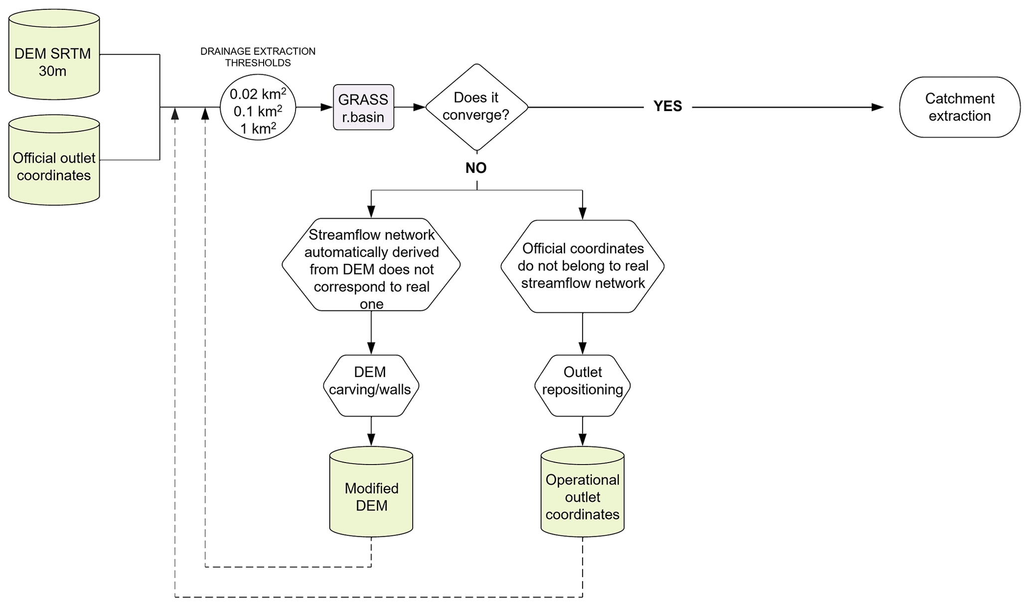
As expected, the procedure for catchment boundary delineation is generally very accurate where the differences in elevation are quite marked (i.e., in alpine areas). Thus, the only manipulation required is the repositioning of the catchment outlet, which, in our case, is always positioned at the gauging stations. However, this method does not always provide the real drainage directions in flat areas, and it is therefore necessary to manually force the DEM to correct the total contributing area (TCA) map built by the r.basin procedures, a practice commonly known as stream burning (Lindsay, 2016). This operation is performed individually, when needed, by comparing the unconstrained river network produced by r.basin with the reference one provided by ISPRA. This quality checking was iteratively repeated by carving rivers or inserting artificial barriers to force the stream onto the correct path. The extent of this operation, i.e., the location(s) and length(s) of the carved or (and) walled portion(s), is unique for each area; for this reason, this operation requires an individual assessment. The procedure described above is depicted in the flow chart in Fig. 1.
The catchment boundaries resulting from the delimitation are finally made available in vector format in the WGS84 UTM32 N (EPSG 32632) coordinate system. The catchment boundaries were used as masks to clip several layers of climatological and soil-related attributes. Moreover, the provision of this geographic information will allow users to expand this database by computing other descriptors using possible new gridded datasets.
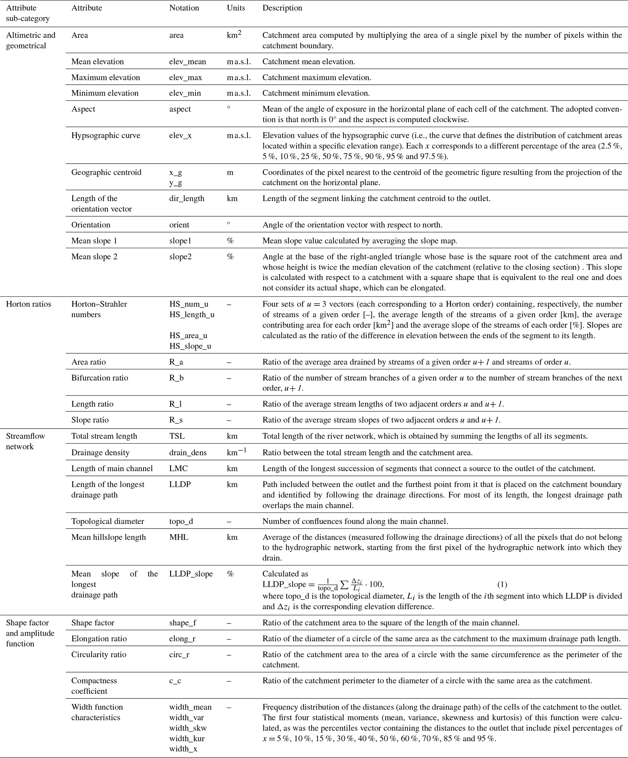
Table 1List of geomorphological attributes, with a brief description of each and an indication of the algorithm/add-on used for its computation. All the attributes are computed by processing the SRTM DEM at 30 m resolution with the r.basin add-on, which takes advantage of other the GRASS GIS algorithms mentioned at the beginning of Sect. 3.3.
3.3 Geomorphological catchment attributes
Geomorphoclimatic information, along with soil characteristics, is essential when trying to characterize how the catchment stores and transports water both on and below the surface. In this work, we first selected from the literature a large set of morphological attributes that can be directly obtained by processing the 30 m resolution STRM DEM. Automatic procedures based on the GRASS add-ons r.basin, r.stat, r.slope.aspect, r.stream.stats (Jasiewicz, 2021) and r.accumulate (Cho, 2020) are used for this computation. This leads to 61 geomorphological attributes (see Table 1 for a complete description).
The provision of this set of 61 different attributes for more than 600 catchments nationwide represents one of the strengths of the FOCA dataset. Comparing it to other relevant examples that we found in the literature, such as the CAMELS or the LamaH-CE datasets, one realizes that they include only a limited number of geomorphological descriptors and focus mainly on climatic, hydrologic, land-cover, soil and geological indices. As an example, in the CAMELS developed for the US (Addor et al., 2017) or for Brazil (Chagas et al., 2020), only basic topographic characteristics related to outlet coordinates, the catchment area, the mean elevation and mean catchment slopes are reported. In the LamaH-CE dataset (Klingler et al., 2021), some additional geomorphological attributes were included, such as the median basin elevation, the range of catchment elevations, the elongation ratio, the horizontal distance from the farthest point of the catchment to the corresponding gauge, and the drainage density. The inclusion of other descriptors in LamaH-CE was motivated by the need to know both the shape of the catchments and the stream network influence on runoff formation. We believe that the small number of descriptors included in previous works could be insufficient to fully characterize areas with complex river networks. Here we stress the need to carefully characterize the catchments from a geomorphological point of view too, especially when a high percentage of the catchments considered are located in mountainous areas.
To further highlight the importance of this latter point, we underline that in the Italian context, which is the focus of this work, non-standard geomorphological parameters have already been demonstrated to be significant in several applications of statistical hydrology, such as the regionalization of the flood frequency curves for NW Italy developed by Laio et al. (2011). In that case, the proposed regression models consider geomorphological parameters like the area, the mean elevation, the length of the longest drainage path, the length of the orientation vector and the catchment outlet coordinates as covariates. In a revised version of the methodology (Ganora et al., 2014), the minimum elevation and the shape factor were also significant covariates. In Ganora et al. (2023), a non-dimensional flood reduction function to estimate design hydrographs for ungauged catchments was obtained with a multiple linear regression model that included the longest drainage path length and the slope of the catchment, the average catchment elevation, and the fourth statistical moment of the width function.
Moving to a broader context, the literature suggests that among the factors that govern the catchment's hydrological response during the process of rainfall–runoff transformation, the catchment's geomorphological features have been well represented (see, e.g., Nagy et al., 2021; Ravazzani et al., 2019). The synthesis of the basin response function from physical basin characteristics becomes crucial in ungauged catchments (Singh et al., 2013). Finally, most of the formulations available in the literature to estimate the response time when no runoff data are available typically contain a characteristic length and the slope of the catchment or the main channel (e.g., Chow, 1962; Kirpich, 1940; Sheridan, 1994), which are not readily available from the other abovementioned databases.
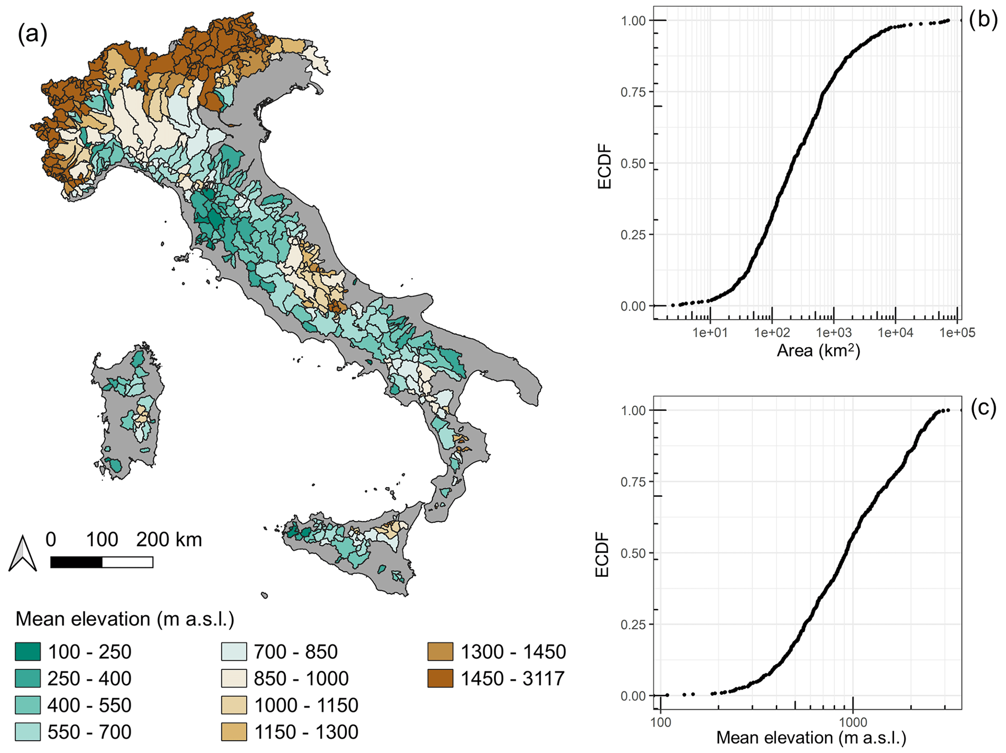
Figure 2Mean elevation of the 631 catchments (a) and empirical cumulative distribution functions (ECDFs) of some key catchment attributes: area (b) and mean elevation (c). Administrative boundaries: GADM v3.6.
The catchments included in the FOCA dataset cover a wide variety of morphological features and a considerable elevation range (Fig. 2a). Figure 2 also shows the empirical cumulative distribution functions (ECDFs) of some key catchment attributes: the area (Fig. 2b) and the mean catchment elevation (Fig. 2c). Figure 2 also reveals the limited number of catchments with outlets close to the sea. However, there is a reason behind this absence: the 631 chosen catchments that we considered are those for which peak or daily discharges are available and are therefore all included in the Catalogo delle Piene dei Corsi d'acqua Italiani. This implies that all the gray areas are ungauged; they could be included in the dataset but only if gauging stations were to be installed in the near future.
3.4 Quality check of the geomorphic data
To provide a robust set of catchment features, we have checked the consistency between this new dataset and the previously published one (Claps et al., 2020a, b, c) in terms of catchment areas, which were mostly based on the values published in the hydrologic yearbooks and in Pubblicazione no. 17. In order to set the level of accuracy of the procedures that we used, a 10 % maximum deviation of the difference (positive or negative) was considered acceptable. All the catchments for which the discrepancy is greater than 10 % have been individually re-examined, as described in Sect. 3.2. In some cases, the discrepancy was found to derive from a small shift of the catchment outlets upstream or downstream of a confluence, thus including or excluding relevant sub-catchments.
Another important check has been made: the difference between the length of the main channel (LMC) of each catchment and the length of the longest drainage path (LLDP) was analyzed. Even though these two attributes are well known to have a strong relationship, this connection was not always found in our data: for some catchments, the two lengths were significantly different, even after a thorough manual check. A threshold of a 3 km difference (corresponding to the value that selects the upper 5 % of the catchments with marked differences) was used to identify those catchments for which the difference in length between LMC and LLDP should be further investigated. For those catchments, manual inspections highlighted a drawback in the GIS procedure that produced LMC and LLDP measurements with unrealistic discrepancies. Two different cases were observed. In one case, the resulting main channel shapefile consisted of a polygonal chain made up of multiple features that needed to be merged into one. In the other case, multiple LLDPs that differed from each other by no more than 100 m (2–3 pixels) were identified for the same catchment. In the latter case, one LLDP was manually chosen and the other ones were removed. We also observed that the two situations could occur simultaneously.
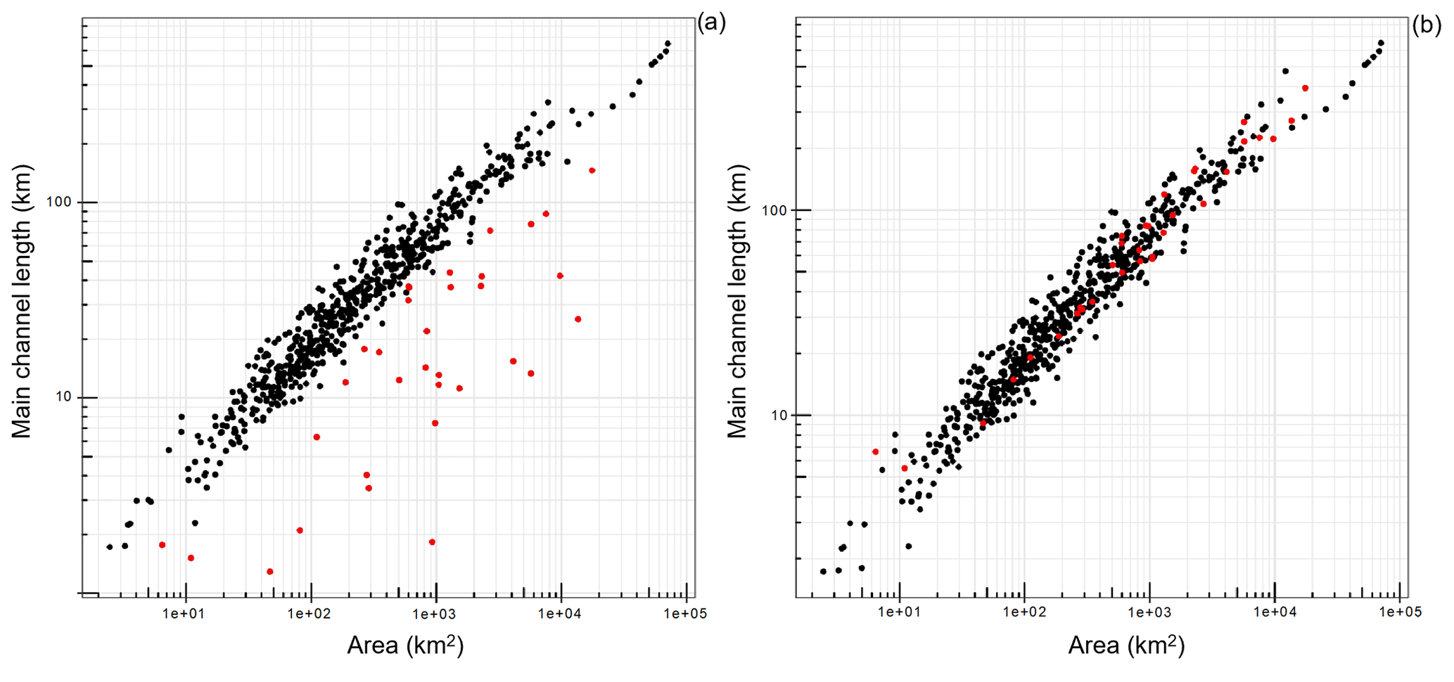
Figure 3Scaling law between main channel length and basin area for the 631 catchments before (a) and after (b) the quality-control procedure for LLDP and LMC.
To get a general feel for the consistency of these two attributes, some scaling laws for the drainage network can be employed. One of the best-known is Hack's law (Hack, 1957; Eq. 3), which reads
where the coefficients α and β vary depending on the study area. A log-log scatter plot between main channel length and basin area for all 631 catchments is displayed in Fig. 3, where panels (a) and (b) refer to the results before and after the quality control, respectively. By means of the abovementioned comparisons, we were able to double-check the consistency between the two attributes; we found errors of up about 20 km, which we checked and corrected.
This section describes the work done and the datasets used to evaluate area-averaged catchment attributes concerning the soil, vegetation, climate and related extremes (for both rainfall and discharges).
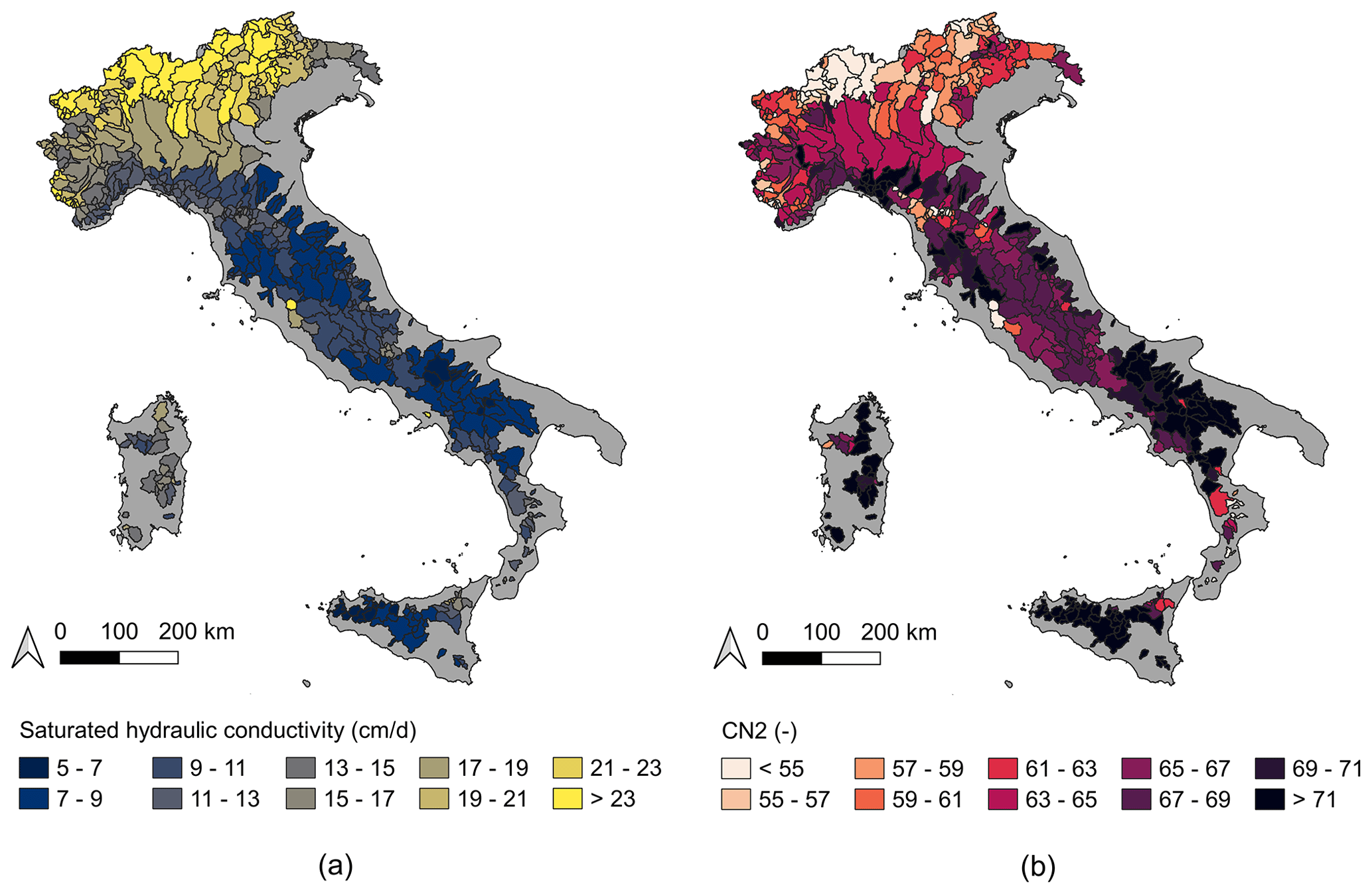
Figure 4Mean areal values of the saturated hydraulic conductivity (a) and the curve number in average conditions, i.e., CN2 (b). Administrative boundaries: GADM v3.6.
For all the attributes, a spatial average value is provided, along with an additional assessment of the spatial variability in terms of the (spatial) coefficient of variation. On the other hand, the temporal variability is not considered here. The only exceptions are the coefficient of variation of the NDVI (normalized difference vegetation index) and the coefficient of variation of the rainfall regimes, which is introduced later and is described in Table 4. The spatial coefficient of variation can thus be considered a proxy for the uncertainty associated with the use of a mean value for the entire catchment. This statistic is additional information that is not usually reported in the CAMELS datasets, but it represents added value here, especially for a nation with such a complex geomorphology and climate as Italy.
All the attributes that will be described hereafter are affected by different sources of uncertainty that may or may not be quantified. To avoid the negative influence that resampling of the original data (available at different spatial resolutions) to a standard specific resolution could have on the results, in this work we used input data with an adequate resolution in relation to the type of information, so we avoided resampling. Moreover, when dealing with a raster obtained through the spatial interpolation of at-site values, the spatialization method could introduce a certain level of uncertainty at the local scale, which could be quantified in pixels where a measurement was present. For the input data that we used, information about measurement or interpolation uncertainty is not always available, since we used several raster maps produced by other research groups. This is the case for land cover, NDVI and climatological data. Information about the uncertainty of the soil data that we used is available in Hengl et al. (2017). When referring to datasets produced by the authors involved in the creation of FOCA (discharge and rainfall extremes; see Sects. 4.2 and 4.3), some additional information is provided.
4.1 Soil, land cover and NDVI catchment attributes
In this subsection, different rasterized information is analyzed to provide area-averaged values. The spatial resolutions of the raw data range from 100 to 1000 m, and the data are not resampled at the same resolution before computing the average values.
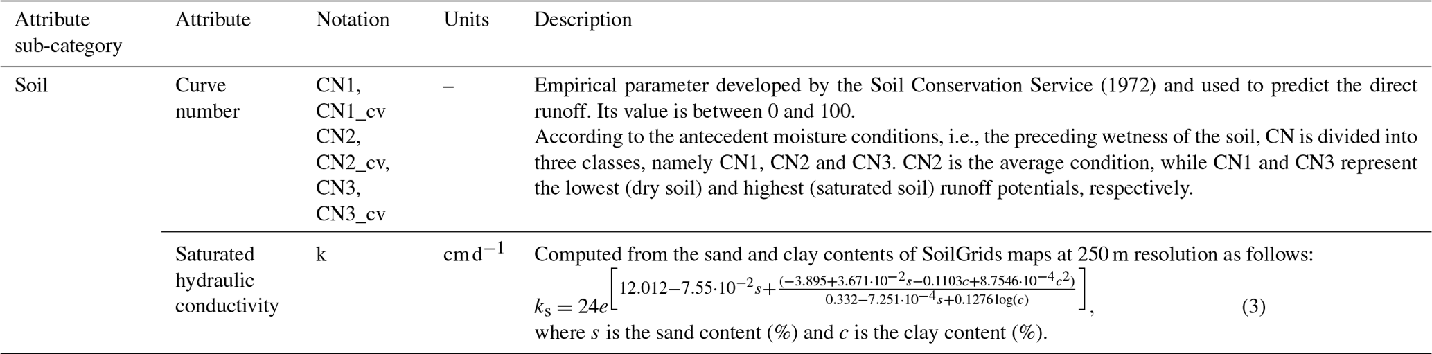
Soil descriptors included in the FOCA dataset can provide information connected to an area-averaged estimate of the soil permeability conditions. These descriptors are the mean areal values of the curve number (Soil Conservation Service, 1972) and of the saturated hydraulic conductivity.
The curve number is an empirical parameter used to evaluate the portion of the total rainfall that becomes the net rainfall in a flood event. The values used in this study were taken from a national-scale cartography produced by Carriero (2004) at 250 m resolution, consistent with the work of Ganora et al. (2013). Since this dataset is currently not available online, it was also included in the dataset in the form of a raster map to grant replicability and thus allow researchers to perform the same study or extend this one to other catchments. Three types of curve numbers are defined, which relate to three different antecedent wetness conditions – dry, average and wet, respectively – of the soils. For each curve number type, we provided the mean value and the (spatial) coefficient of variation.
To derive a feature that approximates soil permeability features, we started from soil texture fraction maps derived from SoilGrids (Hengl et al., 2017; available at https://soilgrids.org/, last access: 23 October 2023). These cartographies map the spatial distribution of soil properties across the globe at 250 m spatial resolution and at seven standard depths ranging from 0 to 200 cm. SoilGrids maps are based on over 230 000 soil profile observations from the WoSIS (World Soil Information Service) database (Batjes, 2009). Soil texture information was derived from these maps after averaging across the first 30 cm of depth, a value consistent with the hydrological purposes of this work. Based on the sand and clay contents, we derived the saturated hydraulic conductivity using the pedo-transfer function proposed by Saxton et al. (1986; Eq. 3).
The seven soil descriptors (six related to the curve number and one related to the saturated hydraulic conductivity) that we considered are listed in Table 2.
Figure 4 provides a snapshot map of the catchment-averaged soil parameter values. The resulting spatial distribution of the saturated hydraulic conductivity (Fig. 4a) illustrates that the soil properties vary significantly upon moving from the north to the south of Italy and reflects the high clay content characterizing the soils of the Apennine basins. The same level of difference is not visible in the CN2 values (Fig. 4b), essentially because they reflect the geological and land-use (not soil) information.
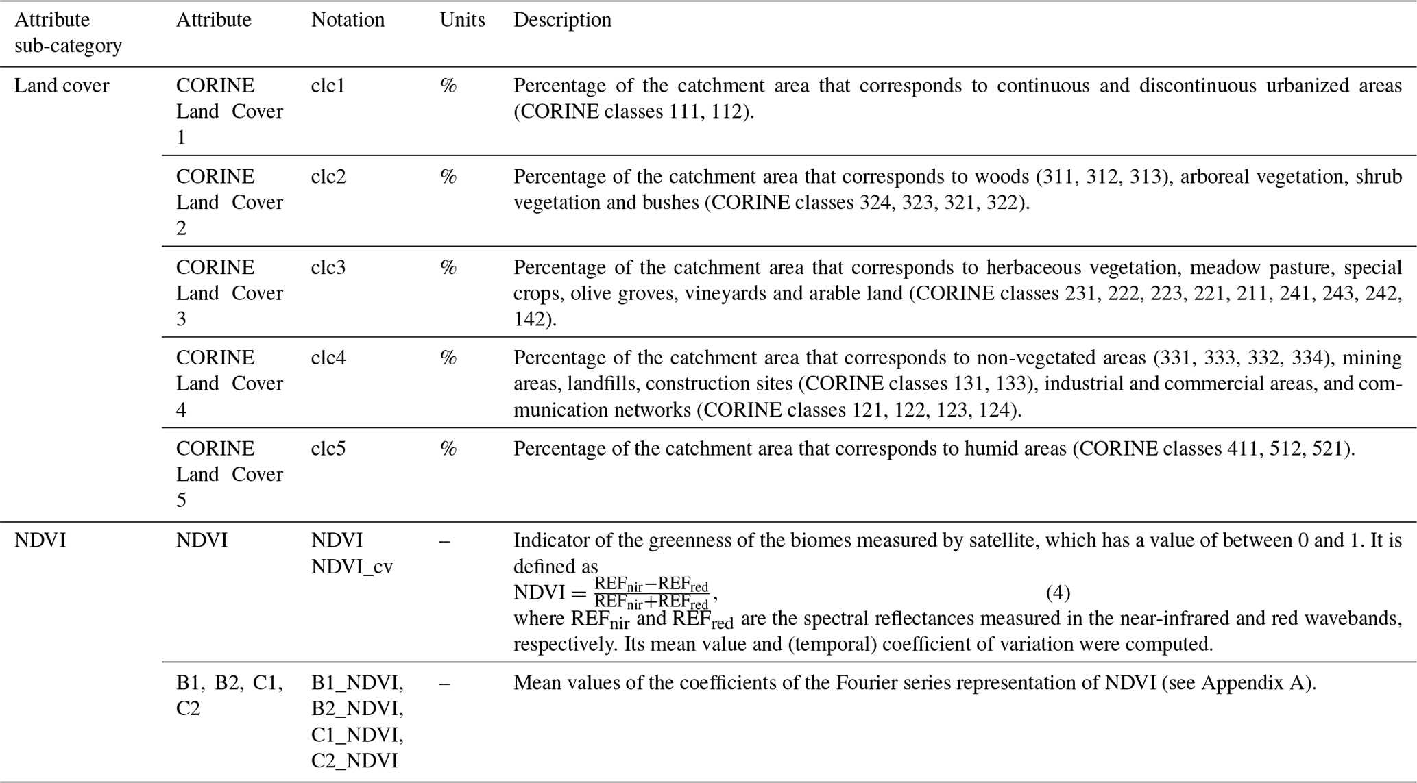
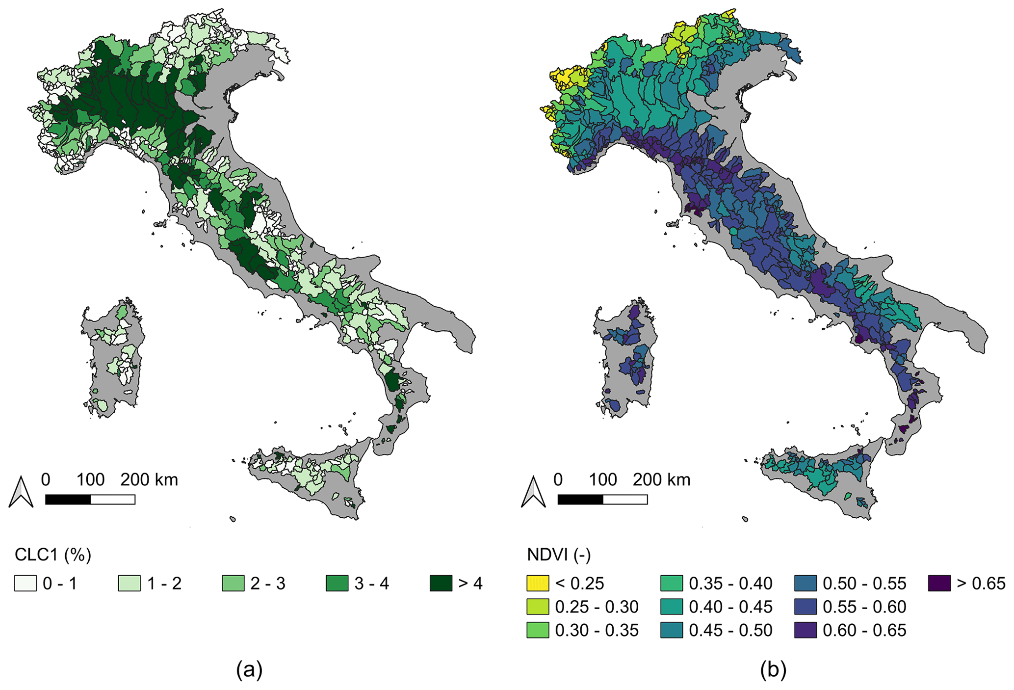
Figure 5Spatial variability of the percentage of clc1 (a) and mean areal NDVI (b). Administrative boundaries: GADM v3.6.
Land cover characteristics at 100 m resolution are extracted from the 44 classes of the third level of CORINE Land Cover 2018 (available at https://land.copernicus.eu/, last access: 23 October 2023). In particular, five land indices obtained by merging similar classes are considered here. The five land indices are outlined in Table 3. A map of one of the classes is provided in Fig. 5a: it displays an overview of the percentage of urbanized areas, thus providing some information related to the relevance of anthropogenic settlements within the catchments. As expected, the vegetation coverage is lower in high-elevation and cold regions (i.e., the Alps), which are also regions with low percentages of urbanized areas.
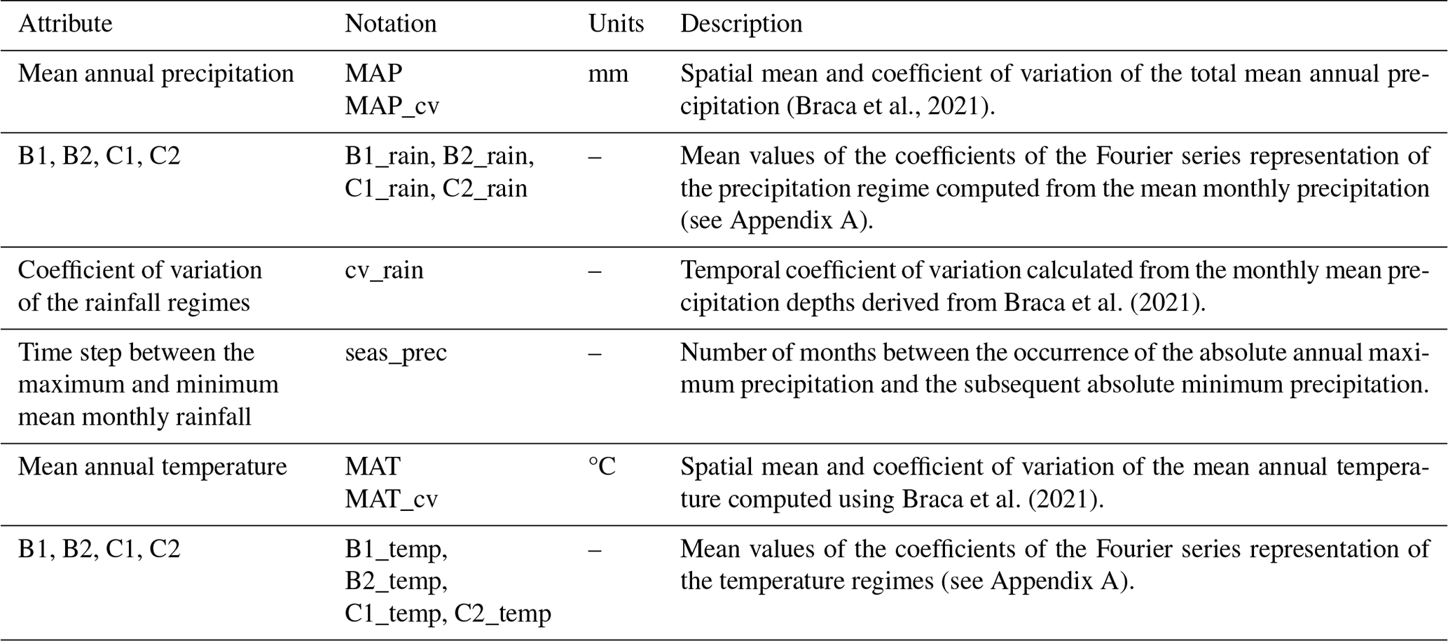
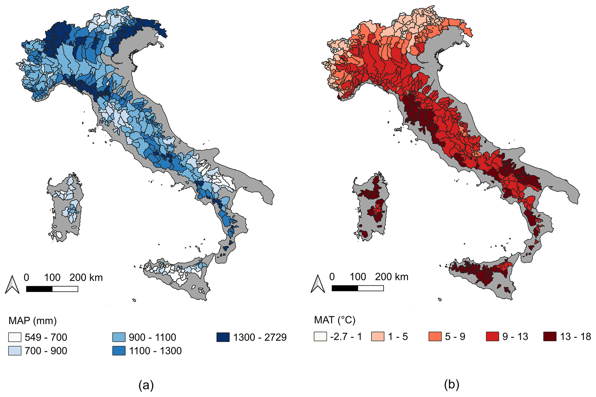
Figure 6Spatial representations of the mean annual precipitation (a) and mean annual temperature (b). Administrative boundaries: GADM v3.6.
We also computed multi-temporal indicators of the NDVI (normalized difference vegetation index) maps, whose data are provided by the Copernicus Land Monitoring Service (available at https://land.copernicus.eu/, last access: 23 October 2023). The NDVI is an index that shows whether the area under investigation contains live green vegetation and shows its overall health. We used the values of the Long Term Statistics (LTS) NDVI V3.0.1 of the Copernicus service (with a 1 km spatial resolution), which are mean NDVI observations over the period 1999–2019 for each of the 36 periods of 10 days per year, resulting in 36 raster maps. These maps were used to compute the mean NDVI value, the (temporal) coefficient of variation of the NDVI and the spatio-temporal mean NDVI regime. The NDVI regime is a graphical representation of the multi-temporal mean calculated over 36 time intervals, each spanning 10 d. To synthetically characterize the latter, a Fourier series representation was used, which allows the shape of the regime to be described with fewer parameters (four in total) than the 36 average values (each for a different 10 d period) from which it is composed. A more detailed description of the four parameters that describe the coefficients of the Fourier series that represent the NDVI regime is reported in Appendix A.
After this data preparation, catchment boundaries were used to extract a total of 11 land cover and NDVI attributes, as listed in Table 3. The mean NDVI is mapped in Fig. 5b to provide some insight into the variation of the mean greenness of the biomes.
4.2 Climatological catchment attributes
State-of-the-art national-scale datasets at 1 km resolution have been used for the evaluation of several climatological attributes, as described below.
Mean monthly precipitation information is taken from the BIGBANG (Bilancio Idrologico GIS BAsed a scala Nazionale su Griglia regolare; Braca et al., 2021) 4.0 dataset, which covers the 1951–2019 period. BIGBANG is obtained by means of the spatial interpolation of rain gauge measurements at 1 km resolution, and integrates, only over limited areas and for certain years, the spatial interpolation produced by ARCIS (Archivio Climatologico per l'Italia Centro Settentrionale; Pavan et al., 2019). Mean monthly temperature data are also derived from this dataset. Both mean monthly precipitation depths and mean monthly temperature data are processed to compute the mean coefficients of the Fourier series that approximate the precipitation and temperature regimes (four coefficients for rainfall and four for temperature; see Appendix A).
This dataset is also used to compute the mean annual precipitation (MAP) and the mean annual temperature (MAT).
Catchment boundaries were used to clip the abovementioned precipitation and temperature maps and obtain spatial averages for the 14 climatological attributes listed in Table 4.
Upon presenting the results, one can notice in Fig. 6a that the mean annual precipitation (MAP) is higher in mountainous regions, with the largest values seen in the Alps. The same areas also show a low mean annual temperature (MAT; Fig. 6b).
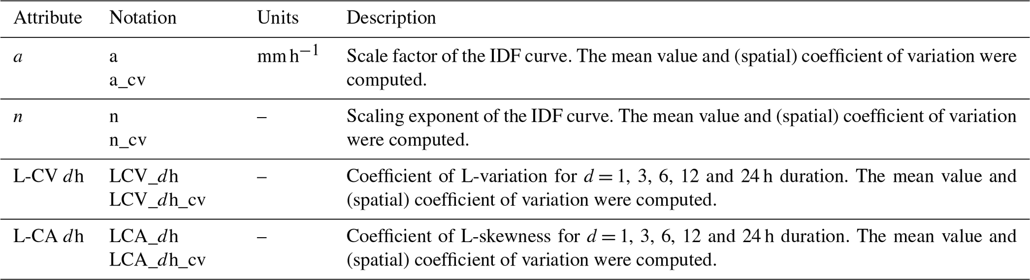
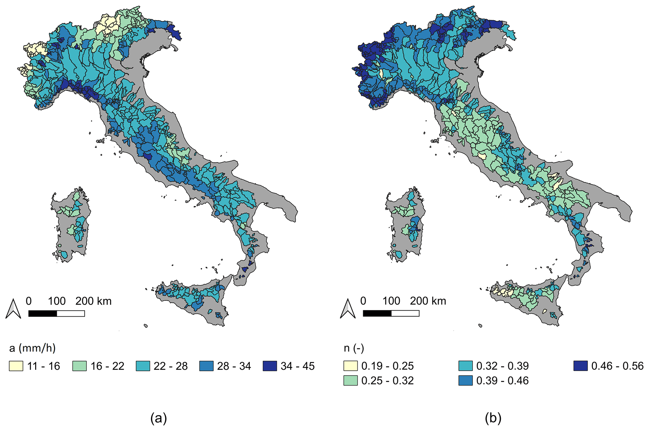
Figure 7Spatial representations of the spatial averages of parameter a (a) and parameter n (b) of the ID curves. Administrative boundaries: GADM v3.6.
4.3 Extreme rainfall catchment attributes
With respect to other national databases, like the LamaH-CE dataset (Klingler et al., 2021), one of the main novelties of this work is the introduction of information related to parameters of the sub-daily precipitation extremes. This inclusion was made possible thanks to the availability of a rich collection of in situ data that are characterized by a much greater accuracy when capturing extremes compared to reanalysis data like the ERA5 and ERA5-Land datasets (Muñoz Sabater, 2019) widely used in the creation of other datasets. The annual maximum rainfall depths used to derive spatial extreme rainfall statistics are obtained from the Improved Italian – Rainfall Extreme Dataset (I2-RED; Mazzoglio et al., 2020). This dataset consists of official and quality-controlled short-duration (1, 3, 6, 12 and 24 h) annual maximum rainfall depths recorded by more than 5200 rain gauges across Italy between 1916 and 2019. The stations were subjected to a quality-control procedure to correct errors in the plano-altimetric positions, duplicates and incorrect rainfall measurements (Mazzoglio et al., 2020). This FOCA dataset represents the first national-scale collection of mean extreme rainfall catchment attributes. Thanks to FOCA, it is now possible to perform simple regional and national hydrological studies without the need to retrieve information from 21 different agencies, as mentioned in the “Introduction”. Due to the complex data policy that regulates the data collected by the hydrological agencies (most of them only provide the data free of charge for research purposes, while people interested in using them for commercial purposes are requested to pay), we were not allowed to include the annual maxima time series in the FOCA dataset. However, nationwide maps of the parameters allowing the computation of the IDF (intensity–duration–frequency) curves have been prepared and made freely available within the FOCA dataset.
Rainfall data and related statistics are processed at 250 m resolution with the R function autokrige (Hiemstra and Skoien, 2023). This performs automatic ordinary kriging using the variogram that best fits the data, which is automatically generated by the R function autofitVariogram. The rainfall statistics obtained with this procedure are
-
the scale factor a and the scaling exponent n of the average intensity–duration (ID) curves, which are obtained by linear regression of the logarithm of the average rainfall depth hd for the durations of 1 to 24 h against the logarithm of the duration, where
-
the coefficient of L-variation (L-CV) for the durations of 1 to 24 h, which is evaluated with Eq. (6) of Laio et al. (2011)
-
coefficient of L-skewness (L-CA) for the durations of 1 to 24 h, which is evaluated with Eq. (7) of Laio et al. (2011).
Time series with at least 10 years of data were used to evaluate the parameters a and n, while series with 20 and 30 years of data were used for L-CV and L-CA, respectively. The different record lengths were selected because higher-order statistics cannot be evaluated from short time series (Koutsoyiannis, 2019). These maps represent the first attempt to reconstruct and represent updated extreme rainfall statistics across Italy following similar releases for Switzerland (i.e., the Hydrological atlas of Switzerland, available at https://hydrologicalatlas.ch/, last access: 23 October 2023), Austria (i.e., the Hydrological atlas of Austria; Fürst et al., 2009), Germany (i.e., the KOSTRA-DWD or Coordinated heavy precipitation regionalization and evaluation of the DWD, available at https://www.dwd.de/DE/leistungen/kostra_dwd_rasterwerte/kostra_dwd_rasterwerte.html, last access: 23 October 2023), the United States (i.e., NOAA Atlas 14, available at https://www.weather.gov/owp/hdsc_currentpf, last access: 23 October 2023 and at https://hdsc.nws.noaa.gov/hdsc/pfds/, last access: 23 October 2023), Hawaii (i.e., the Rainfall atlas of Hawai'i, available at http://rainfall.geography.hawaii.edu/, last access: 23 October 2023) and Canada (CSAGroup, 2019).
Table 5 summarizes the characteristics of the attributes computed and averaged over the 631 catchments.
A discussion of the overall spatial and temporal variability of the rainfall extremes is available in Mazzoglio et al. (2020, 2022a, b, 2023). What is useful to comment on here is the result of the spatial averaging of the parameters a and n at the catchment scale (Fig. 7a and b). The parameter a can be combined with n to obtain the mean rainfall for different durations (1 to 24 h). The first one represents the mean rainfall extremes of 1 h duration: the higher the value of a, the higher the intensity of short-duration rainfall extremes over the catchments. This parameter is particularly relevant for small catchments with a characteristic time lag of the order of 1 h. If Fig. 7 is compared to Fig. 2, we can see a modest correlation between a and elevation (the reverse orographic effect; Avanzi et al., 2015; Mazzoglio et al., 2022a, 2023). One can also notice that the regions where the most severe short-duration rainfall events occur (Fig. 7a) are different from those that present a higher MAP (Fig. 6a), which is a characteristic of the Mediterranean climate (Mazzoglio et al., 2022a).
In terms of the assessment of the uncertainty associated with the spatial average values, Fig. 8 provides interesting insights, as it shows the standard deviation of the kriging estimates of the parameter a in each individual pixel. The figure shows an almost uniform spatial distribution of the interpolation uncertainty, with higher values found near the coastline (due to the lower station network density) and lower values found where the station density is high. Thus, this map not only serves to show the interpolation uncertainty but also provides information on the rain gauge density throughout the country.
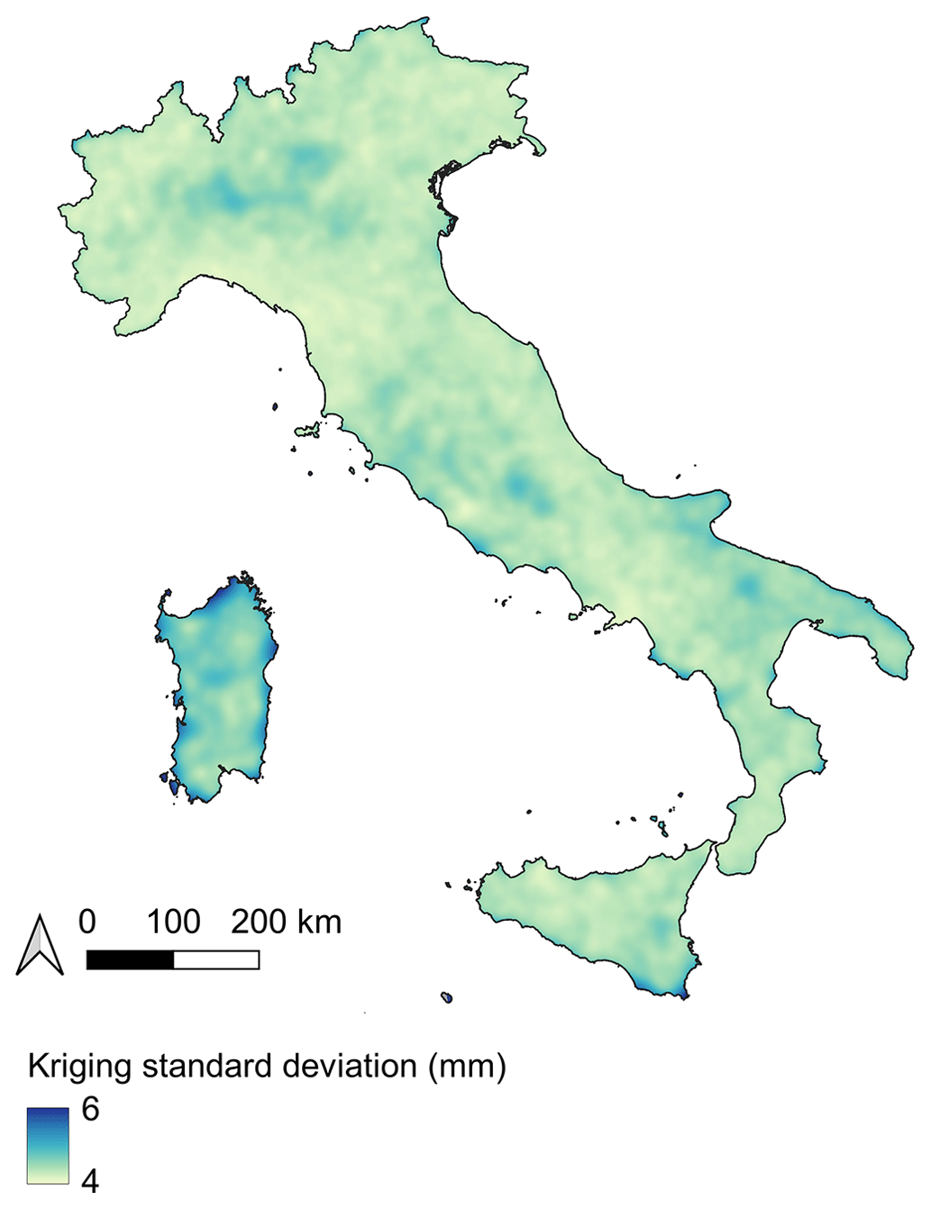
Figure 8Standard deviation of the kriging estimate of the parameter a. Administrative boundaries: GADM v3.6.
4.4 Peak and daily discharge collections
As outlined in Sect. 2, the peak and daily discharges from each gauging station come from Claps et al. (2020a, b, c), which is the most up to date systematic flood collection in Italy. Until the 1970s, the data reflect most of the content of Pubblicazione no. 17 of the SIMN (Servizio Idrografico, 1980). After that, a consistent integration was carried out by merging data from different sources (such as Bencivenga et al., 2011; Barbero et al., 2012; Hall et al., 2015; Brath et al., 2017; Settore Idrologico e Geologico Regionale, 2022; ARPA Lombardia Sistema Informativo Idrologico, 2023) using the same database set up for the CUBIST project (Claps et al., 2008).
The provision of that information in this paper (in terms of both the time series and of their statistics, like the mean values of the flood peaks, Q_p) offers the opportunity to fully characterize the climatology of the extremes for the catchments upstream of the gauging stations. The uncertainty of observed discharge values cannot be reported since it is a piece of information that is not available to the public. In essence, before their publication in the hydrological yearbooks, these data were validated through the application of the corresponding rating curves for every year of measurement. However, it is not possible to rate the uncertainty of the level-to-discharge conversions, which were made decades ago. This would involve accounting for very site-specific technical issues that can be dealt with only in strict cooperation with the offices where the peak discharge values were validated, and it would need to be done for each and every measurement section.
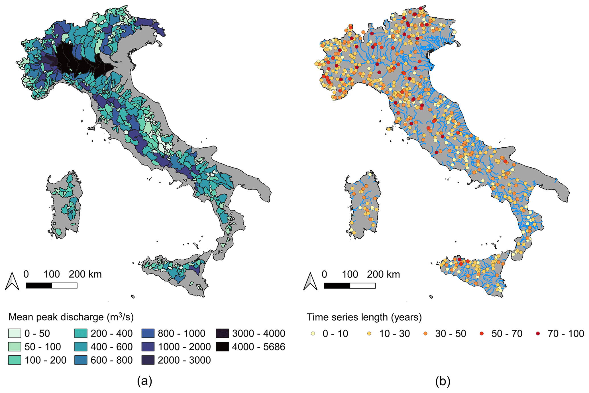
Figure 9Spatial distributions of the mean peak discharge (a) and discharge time series length (b). Administrative boundaries: GADM v3.6.
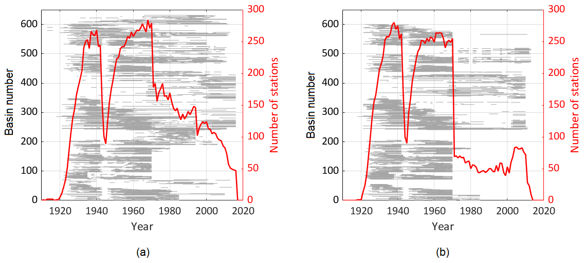
Figure 10Temporal availability of the peak (a) and daily (b) discharge. Each gray line represents a time series; in these time series, gray identifies available records while white indicates missing data. The bold red line identifies the total number of measurements available for each year.
The spatial variability of the mean annual flood is shown in Fig. 9a, in which one can recognize the presence of nested sub-catchments resulting from the presence of different measurement stations located along the river path. This situation is particularly evident in the northwest of Italy, where different small mountainous sub-catchments of the Po basin are highlighted, while the Po basin itself is the partially visible catchment depicted in black. To get an idea of the lengths of the discharge time series available, one can refer to Fig. 9b: the different dot colors show that most of the longer time series (> 50 years) are generally available in North and Central Italy. Moreover, while the reference period covered by the dataset dates from 1911 to 2016, the time series are fragmented and characterized by different time coverages and thus do not characterize the entire interval (Fig. 10). The decreasing number of time series in recent decades is due to the lack of quality-controlled discharge data published by the regional hydrological agencies, which is mostly due to the unavailability of updated rating curves. In most cases, the regional agencies are now only publishing water levels, while information about discharges is often missing.
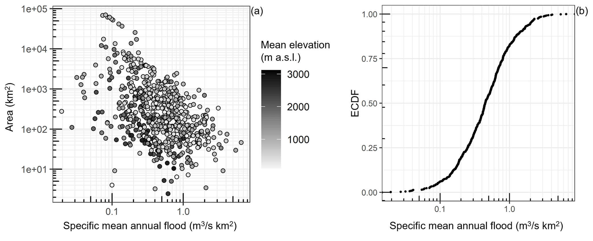
Figure 11Relationship between catchment area, specific peak discharge and mean elevation (a) and the empirical cumulative distribution function (ECDF) of the specific mean annual flood (b).
The catchments cover a wide variety of morphological features. Figure 11 shows the empirical cumulative distribution function (ECDF) of the specific mean annual flood (i.e., the ratio between the mean peak discharge Q_p and the catchment area; Fig. 11b). The relationship between the area, the specific mean annual flood and the mean catchment elevation is represented in Fig. 11, which shows how the Italian catchments are characterized by different hydrological regimes and a modest dependence of the mean elevation on the specific peak discharge. Catchments with a high mean elevation (from 2000 to more than 3000 ) cover a wide range of possible specific mean annual floods, but the interval is smaller than that characterizing catchments located at lower elevations.
The dataset detailed in this paper is available at https://doi.org/10.5281/zenodo.10446258 (Claps et al., 2023). It contains all the catchment boundaries and related catchment attributes described before. In case of future updates, to access the latest version of the database, readers can refer to https://doi.org/10.5281/zenodo.8060736 (Claps et al., 2023) to download the most recent version.
In this work, we have presented FOCA (Italian FlOod and Catchment Atlas), a collection of attributes of 631 Italian river catchments derived from data sources that comply with the following criteria: (a) nationwide coverage; (b) consistency in data quality (i.e., no regional or local biases); and (c) adequate original resolution in relation to the type of information.
FOCA represents the most up to date collection of catchment boundaries and related attributes at the national scale for Italy. It summarizes features related to climate (discharge, rainfall and temperature), geomorphology, soil and land use. The dataset covers an overall area representative of most of the landscapes of Italy, including the mountainous ones (elevations ranging from 0 to 4800 m). One of the main novelties with respect to other national-scale datasets is the inclusion of a rich set of geomorphological and extreme rainfall attributes. The second notable novelty is the inclusion, in the same dataset, of the most up to date information regarding extreme rainfall and discharge.
As mentioned before, Italy shows very wide variability in climate, land and morphological features, and this peculiarity emerges from this new dataset. Figure 2b shows that the FOCA dataset includes catchments with significantly different areas, with small-to-medium ones prevailing: 105 out of 631 catchments have an area of less than 50 km2, and 300 out of 631 catchments have an area of less than 200 km2. In addition, 279 out of 631 catchments have a mean elevation higher than 1000 , highlighting that, despite the existence of some large plains, Italy is a mountainous country. On the other hand, in the large catchments in the north of Italy, the spatial averaging operation over the catchment area becomes less significant, as it is evaluated over an area within which significantly different features coexist.
A key decision that we had to take while developing FOCA was whether to use local or global/quasi-global datasets or both. The use of global datasets facilitates the comparison of the results obtained in large-scale hydrology works, even when continental analyses are performed. However, local datasets are, without a doubt, characterized by higher-quality information. In this work, we decided to opt for the second approach, selecting the best possible data for each variable, prioritizing local information, and resorting to global data in only a few cases. The availability of digital information on the catchment boundaries allows users to evaluate the mean areal values of other variables, such as evapotranspiration and snow cover, using their own models or other large-scale reanalysis datasets, like ERA5 and ERA5-Land.
The FOCA dataset provides new opportunities to perform both regional and national-scale studies using catchment shapes and attributes extracted using a common framework and subjected to the same quality-control procedure. Information about the algorithms used in this work are also reported in Sect. 3 to ensure replicability and allow the calculation of the attribute characteristics for any ungauged basin. Moreover, the database provides the opportunity to investigate how catchment attributes control river flows and allows the improvement of data-intensive investigations, such as performing predictions for ungauged catchments.
The rainfall, temperature and NDVI regimes are described using Fourier series, which allows the shape of the regime to be reconstructed using a reduced number of parameters compared to the 12 different monthly values (or the 36 values for 10 d periods in the case of the NDVI) used to describe it. According to Fourier's theorem, a wave of period τ and pulse ω = can be described as
where t is the time, A0 is the mean of f(t) over t, N is the number of harmonics, Ai is the harmonic amplitude and ϕi is the phase. In the case of two harmonics, Eq. (6) can be written as
By separating the variables that depend on the time from those that are not time dependent, we obtain
In this analysis, we evaluated B1, B2, C1 and C2 with the ordinary least-squares method (see Eqs. 9 to 12).
The equation can be further simplified by assuming the mean A0 to be null and solving it for τ=2π.
PC: conceptualization, funding acquisition, methodology, project administration, resources, supervision, writing – review and editing. GE: conceptualization, data curation, formal analysis, investigation, methodology, software, validation, visualization, writing – original draft preparation, writing – review and editing. DG: conceptualization, methodology, writing – review and editing. PM: conceptualization, data curation, formal analysis, investigation, methodology, software, validation, visualization, writing – original draft preparation, writing – review and editing. IM: conceptualization, data curation, formal analysis, investigation, methodology, software, validation, visualization, writing – original draft preparation, writing – review and editing.
The contact author has declared that none of the authors has any competing interests.
Publisher's note: Copernicus Publications remains neutral with regard to jurisdictional claims made in the text, published maps, institutional affiliations, or any other geographical representation in this paper. While Copernicus Publications makes every effort to include appropriate place names, the final responsibility lies with the authors.
This study was carried out within the RETURN Extended Partnership and received funding from the European Union NextGenerationEU (National Recovery and Resilience Plan – NRRP, Mission 4, Component 2, Investment 1.3 – D.D. 1243 2/8/2022, PE0000005) – SPOKE TS2. This study has been partially conducted within the framework of the technical–scientific collaboration agreement signed between the Southern Apennine District Basin Authority and the Consorzio Interuniversitario per l'Idrologia (CINID).
This research has been supported by the RETURN Extended Partnership and received funding from the European Union NextGenerationEU (National Recovery and Resilience Plan – NRRP, Mission 4, Component 2, Investment 1.3 – D.D. 1243 2/8/2022, PE0000005) – Spoke TS2 and by the Southern Apennine District Basin Authority.
This paper was edited by Sibylle K. Hassler and reviewed by Uwe Ehret and Benjamin Kitambo.
Addor, N., Newman, A. J., Mizukami, N., and Clark, M. P.: The CAMELS data set: catchment attributes and meteorology for large-sample studies, Hydrol. Earth Syst. Sci., 21, 5293–5313, https://doi.org/10.5194/hess-21-5293-2017, 2017.
Alvarez-Garreton, C., Mendoza, P. A., Boisier, J. P., Addor, N., Galleguillos, M., Zambrano-Bigiarini, M., Lara, A., Puelma, C., Cortes, G., Garreaud, R., McPhee, J., and Ayala, A.: The CAMELS-CL dataset: catchment attributes and meteorology for large sample studies – Chile dataset, Hydrol. Earth Syst. Sci., 22, 5817–5846, https://doi.org/10.5194/hess-22-5817-2018, 2018.
Andréassian, V., Delaigue, O., Perrin, C., Janet, B., and Addor, N.: CAMELS-FR: A large sample, hydroclimatic dataset for France, to support model testing and evaluation, EGU General Assembly 2021, online, 19–30 April 2021, EGU21-13349, https://doi.org/10.5194/egusphere-egu21-13349, 2021.
ARPA Lombardia Sistema Informativo Idrologico: SIDRO – Sistema Informativo Idrologico, https://idro.arpalombardia.it/it/map/sidro/ (last access: 29 May 2023).
Arsenault, R., Bazile, R., Ouellet Dallaire, C., and Brissette, F.: CANOPEX: A Canadian hydrometeorological watershed database, Hydrol. Process., 30, 2734–2736, https://doi.org/10.1002/hyp.10880, 2016.
Avanzi, F., De Michele, C., Gabriele, S., Ghezzi, A., and Rosso, R.: Orographic signature on extreme precipitation of short durations, J. Hydrometeorol., 16, 278–294, https://doi.org/10.1175/JHM-D-14-0063.1, 2015.
Barbero, S., Claps, P., Graziadei, M., Zaccagnino, M., Saladin, A., Ganora, D., Laio, F., and Radice, R.: Catalogo delle massime portate annuali al colmo del bacino occidentale del Po, Arpa Piemonte, Torino, Italy, 301 pp., ISBN 978-88-7479-112-5, 2012.
Batjes, N. H.: Harmonized soil profile data for applications at global and continental scales: Updates to the 857 WISE database, Soil Use Manage., 25, 124–127, https://doi.org/10.1111/j.1475-2743.2009.00202.x, 2009.
Beighley, R. E. and Gummadi, V.: Developing channel and floodplain dimensions with limited data: a case study in the Amazon Basin, Earth Surf. Proc. Land., 36, 1059–1071, https://doi.org/10.1002/esp.2132, 2011.
Bencivenga, M., Calenda, G., and Mancini, C. P.: Ricostruzione storica delle scale di deflusso delle principali stazioni di misura del bacino del fiume Tevere: il secolo XX, Istituto Poligrafico e Zecca dello Stato, Roma, Italy, 355 pp., 2011.
Braca, G., Bussettini, M., Lastoria, B., Mariani, S., and Piva, F.: Elaborazioni modello BIGBANG versione 4.0, Istituto Superiore per la Protezione e la Ricerca Ambientale – ISPRA, http://groupware.sinanet.isprambiente.it/bigbang-data/library/bigbang40 (last access: 11 March 2024), 2021.
Brath A., Castellarin A., Domeneghetti A., and Persiano, S.: Rapporto sintetico riguardante l'esame critico degli studi idrologici sui bacini delle alpi orientali e dell'appennino settentrionale, DICAM – Università degli studi di Bologna, Bologna, Italy, 2017.
Carriero, D.: Analisi della distribuzione delle caratteristiche idrologiche dei suoli per applicazioni di modelli di simulazione afflussi-deflussi, PhD thesis, Università degli studi della Basilicata, 2004.
Chagas, V. B. P., Chaffe, P. L. B., Addor, N., Fan, F. M., Fleischmann, A. S., Paiva, R. C. D., and Siqueira, V. A.: CAMELS-BR: hydrometeorological time series and landscape attributes for 897 catchments in Brazil, Earth Syst. Sci. Data, 12, 2075–2096, https://doi.org/10.5194/essd-12-2075-2020, 2020.
Cho, H.: A recursive algorithm for calculating the longest flow path and its iterative implementation, Environ. Model Softw., 131, 104774, https://doi.org/10.1016/j.envsoft.2020.104774, 2020.
Chow, V. T.: Hydrologic determination of waterway areas for the design of drainage structures in small drainage basins, University of Illinois Engineering Experiment Station Bulletin No. 462, Urbana, IL, 104 pp., https://core.ac.uk/download/pdf/4814575.pdf (last access: 11 March 2024), 1962.
Claps, P., Barberis, C., De Agostino, M., Gallo, E., Laguardia, G., Laio, F., Miotto, F., Plebani, F., Vezzù, G., Viglione, A., and Zanetta, M.: Development of an Information System of the Italian basins for the CUBIST project, Geophysical Research Abstracts, 10, 2008.
Claps, P., Ganora, D., Apostolo, A., Brignolo, I., and Monforte, I.: Catalogo delle Piene dei Corsi d'acqua Italiani Vol. 1, Ed. CINID., 499 pp., ISBN 978-88-945568-0-3, 2020a.
Claps, P., Ganora, D., Apostolo, A., Brignolo, I., and Monforte, I.: Catalogo delle Piene dei Corsi d'acqua Italiani Vol. 2, Ed. CINID, 537 pp., ISBN 978-88-945568-2-7, 2020b.
Claps, P., Ganora, D., Apostolo, A., Brignolo, I., and Monforte, I.: Catalogo delle Piene dei Corsi d'acqua Italiani Vol. 3, Ed. CINID, 401 pp., ISBN 978-88-945568-4-1, 2020c.
Claps, P., Evangelista, G., Ganora, D., Mazzoglio, P., and Monforte, I.: FOCA (Italian FlOod and Catchment Atlas), Zenodo [data set], https://doi.org/10.5281/zenodo.10446258, 2023.
Coxon, G., Addor, N., Bloomfield, J. P., Freer, J., Fry, M., Hannaford, J., Howden, N. J. K., Lane, R., Lewis, M., Robinson, E. L., Wagener, T., and Woods, R.: CAMELS-GB: hydrometeorological time series and landscape attributes for 671 catchments in Great Britain, Earth Syst. Sci. Data, 12, 2459–2483, https://doi.org/10.5194/essd-12-2459-2020, 2020.
Crespi, A., Brunetti, M., Lentini, G., and Maugeri, M.: 1961–1990 high-resolution monthly precipitation climatologies for Italy, Int. J. Climatol., 3, 878–895, https://doi.org/10.1002/joc.5217, 2018.
Crespi, A., Matiu, M., Bertoldi, G., Petitta, M., and Zebisch, M.: A high-resolution gridded dataset of daily temperature and precipitation records (1980–2018) for Trentino-South Tyrol (north-eastern Italian Alps), Earth Syst. Sci. Data, 13, 2801–2818, https://doi.org/10.5194/essd-13-2801-2021, 2021.
CSAGroup: Technical guide, Development, interpretation, and use of rainfall intensity-duration-frequency (IDF) information: guideline for Canadian water resources practitioners, CSA PLUS 4013:19, CSA group, 2019.
Delaigue, O., Brigode, P., Andréassian, V., Perrin, C., Etchevers, P., Soubeyroux, J.-M., Janet, B., and Addor, N.: CAMELS-FR: A large sample hydroclimatic dataset for France to explore hydrological diversity and support model benchmarking, IAHS-AISH Scientific Assembly 2022, Montpellier, France, 29 May–3 June 2022, IAHS2022-521, https://doi.org/10.5194/iahs2022-521, 2022.
Di Leo, M. and Di Stefano, M.: An open-source approach for catchment's physiographic characterization, Abstract H52E-06 presented at 2013 Fall Meeting, AGU, San Francisco, CA, USA, 9–13 December 2013, H52E-06, 2013.
Farr, T. G., Rosen, P. A., Caro, E., Crippen, R., Duren, R., Hensley, S., Kobrick, M., Paller, M., Rodriguez, E., Roth, L., Seal, D., Shaffer, S., Shimada, J., Umland, J., Werner, M., Oskin, M., Burbank, D., and Alsdorf, D.: The Shuttle Radar Topography Mission, Rev. Geophys., 45, RG2004, https://doi.org/10.1029/2005RG000183, 2007.
Fowler, K. J. A., Acharya, S. C., Addor, N., Chou, C., and Peel, M. C.: CAMELS-AUS: hydrometeorological time series and landscape attributes for 222 catchments in Australia, Earth Syst. Sci. Data, 13, 3847–3867, https://doi.org/10.5194/essd-13-3847-2021, 2021.
Fürst, J., Godina, R., Peter Nachtnebel, H., and Nobilis, F.: The hydrological atlas of Austria – comprehensive transfer of hydrological knowledge and data to engineers, water resources managers and the public, IAHS-AISH P., 327, 36–44, 2009.
Gallo, E., Ganora, D., Laio, F., and Claps, P.: Atlante dei Bacini Imbriferi Piemontesi, Final report of the RENERFOR-ALCOTRA project, Regione Piemonte, Torino (Italy), ISBN 978-88-96046-06-7, 2013.
Ganora, D., Gallo, E., Laio, F., Masoero, A., and Claps, P.: Analisi idrologiche e valutazioni del potenziale idroelettrico dei bacini piemontesi, Final report of the RENERFOR-ALCOTRA project, Regione Piemonte, Torino (Italy), ISBN 978-88-96046-07-4, 2013.
Ganora, D., Laio, F., and Claps, P.: Valutazione probabilistica delle piene in Piemonte e Valle d'Aosta: Metodologia Regionale Spatially Smooth, Politecnico di Torino, Torino (Italy), http://www.idrologia.polito.it/web2/open-data/Dati_Reports_Piemonte/Piene_Prog_Flora_2014.pdf (last access: 11 March 2024), 2014.
Ganora, D., Evangelista, G., Cordero, S., and Claps. P.: Design flood hydrographs: a regional analysis based on flood reduction functions, Hydrolog. Sci. J., 68, 325–340, https://doi.org/10.1080/02626667.2022.2153051, 2023.
Hack, J.: Studies of longitudinal stream profiles in Virginia and Maryland, US Geological Survey Professional Paper, 294-B, United States Government Printing Office, Washington (USA), 1, 1957.
Hall, J., Arheimer, B., Aronica, G. T., Bilibashi, A., Boháč, M., Bonacci, O., Borga, M., Burlando, P., Castellarin, A., Chirico, G. B., Claps, P., Fiala, K., Gaál, L., Gorbachova, L., Gül, A., Hannaford, J., Kiss, A., Kjeldsen, T., Kohnová, S., Koskela, J. J., Macdonald, N., Mavrova-Guirguinova, M., Ledvinka, O., Mediero, L., Merz, B., Merz, R., Molnar, P., Montanari, A., Osuch, M., Parajka, J., Perdigão, R. A. P., Radevski, I., Renard, B., Rogger, M., Salinas, J. L., Sauquet, E., Šraj, M., Szolgay, J., Viglione, A., Volpi, E., Wilson, D., Zaimi, K., and Blöschl, G.: A European Flood Database: facilitating comprehensive flood research beyond administrative boundaries, Proc. IAHS, 370, 89–95, https://doi.org/10.5194/piahs-370-89-2015, 2015.
Hao, Z., Jin, J., Xia, R., Tian, S., Yang, W., Liu, Q., Zhu, M., Ma, T., Jing, C., and Zhang, Y.: CCAM: China Catchment Attributes and Meteorology dataset, Earth Syst. Sci. Data, 13, 5591–5616, https://doi.org/10.5194/essd-13-5591-2021, 2021.
Hengl, T., Mendes de Jesus, J., Heuvelink, G. B. M., Ruiperez Gonzalez, M., Kilibarda, M., Blagotic, A., Shangguan, W., Wright, M. N., Geng, X., Bauer-Marschallinger, B.,Guevara, M. A., Vargas, R., MacMillan, R. A., Batjes, N. H., Leenaars, J. G. B., Ribeiro, E.,Wheeler, I., Mantel, S., and Kempen, B.: SoilGrids250m: global gridded soil informa-tion based on machine learning, PLOS ONE, 12, e0169748, https://doi.org/10.1371/journal.pone.0169748, 2017.
Hiemstra, P. and Skoien, J. O.: Package “automap”, https://cran.r-project.org/web/packages/automap/automap.pdf (last access: 11 March 2024), 2023.
Höge, M., Kauzlaric, M., Siber, R., Schönenberger, U., Horton, P., Schwanbeck, J., Floriancic, M. G., Viviroli, D., Wilhelm, S., Sikorska-Senoner, A. E., Addor, N., Brunner, M., Pool, S., Zappa, M., and Fenicia, F.: CAMELS-CH: hydro-meteorological time series and landscape attributes for 331 catchments in hydrologic Switzerland, Earth Syst. Sci. Data, 15, 5755–5784, https://doi.org/10.5194/essd-15-5755-2023, 2023.
ISPRA: Bacini idrografici principali, ISPRA [data set], http://geoportale.isprambiente.it/dettagli/?uuid=ispra_rm:20101021:123000 (last access: 23 October 2023), 2005a.
ISPRA: Bacini idrografici secondari, ISPRA [data set], http://geoportale.isprambiente.it/dettagli/?uuid=ispra_rm:20101021:120000 (last access: 23 October 2023), 2005b.
Jasiewicz, J.: r.stream.stats, https://grass.osgeo.org/grass82/manuals/addons/r.stream.stats.html (last access: 11 March 2024), 2021.
Kirpich, Z.: Time of concentration of small agricultural watersheds, Civil Eng., 10, 362, 1940.
Klingler, C., Schulz, K., and Herrnegger, M.: LamaH-CE: LArge-SaMple DAta for Hydrology and Environmental Sciences for Central Europe, Earth Syst. Sci. Data, 13, 4529–4565, https://doi.org/10.5194/essd-13-4529-2021, 2021.
Koutsoyiannis, D.: Knowable moments for high-order stochastic characterization and modelling of hydrological processes, Hydrolog. Sci. J., 64, 19–33, https://doi.org/10.1080/02626667.2018.1556794, 2019.
Kratzert, F., Nearing, G., Addor, N., Erickson, T., Gauch, M., Gilon, O., Gudmundsson, L., Hassidim, A., Klotz, D., Nevo, S., Shalev, G., and Matias, Y.: Caravan - A global community dataset for large-sample hydrology, Sci. Data, 10, 61, https://doi.org/10.1038/s41597-023-01975-w, 2023.
Laio, F., Ganora, D., Claps, P., and Galeati, G.: Spatially smooth regional estimation of the flood frequency curve (with uncertainty), J. Hydrol., 408, 67–77, https://doi.org/10.1016/j.jhydrol.2011.07.022, 2011.
Lindsay, J. B.: The practice of DEM stream burning revisited, Earth Surf. Proc. Land., 41, 658–668, https://doi.org/10.1002/esp.3888, 2016.
Lindsay, J. B. and Creed, I. F.: Removal of artifact depressions from digital elevation models: towards a minimum impact approach, Hydrol. Process., 19, 3113–3126, https://doi.org/10.1002/hyp.5835, 2005.
Linke, S., Lehner, B., Ouellet Dallaire, C., Ariwi, J, Grill, G., Anand, M., Beames, P., Burchard-Levine, V., Maxwell, S., Moidu, H., Tan, F., and Thieme, M.: Global hydro-environmental sub-basin and river reach characteristics at high spatial resolution, Sci. Data, 6, 283, https://doi.org/10.1038/s41597-019-0300-6, 2019.
Loritz, R., Stölzle, M., Guse, B., Kiesel, J., Haßler, S., Mälicke, M., Tarasova, L., Heidbüchel, I., Ebeling, P., Hauffe, C., Müller-Thomy, H., Jehn, F. U., Brunner, M., Götte, J., and Rohini, K.: CAMELS-DE: Initiative für einen konsistenten, frei verfügbaren Datensatz für hydro-meteorologische Analysen in Einzugsgebieten in Deutschland (1.2), Zenodo. https://doi.org/10.5281/zenodo.6517142, 2022.
Mazzoglio, P., Butera, I., and Claps, P.: I2-RED: a massive update and quality control of the Italian annual extreme rainfall dataset, Water, 12, 3308, https://doi.org/10.3390/w12123308, 2020.
Mazzoglio, P., Butera, I., Alvioli, M., and Claps, P.: The role of morphology in the spatial distribution of short-duration rainfall extremes in Italy, Hydrol. Earth Syst. Sci., 26, 1659–1672, https://doi.org/10.5194/hess-26-1659-2022, 2022a.
Mazzoglio, P., Ganora, D., and Claps, P.: Long-term spatial and temporal rainfall trends over Italy, Environm. Sci. Proc., 21, 28, https://doi.org/10.3390/environsciproc2022021028, 2022b.
Mazzoglio, P., Butera, I., Claps, P.: A local regression approach to analyze the orographic effect on the spatial variability of sub-daily rainfall annual maxima, Geomatics, Nat. Hazards Risk, 14, 2205000, https://doi.org/10.1080/19475705.2023.2205000, 2023.
Montgomery, D. R. and Foufoula-Georgiou, E.: Channel network source representation using digital elevation models, Water Resour. Res., 29, 3925–3934, https://doi.org/10.1029/93WR02463, 1993.
Muñoz Sabater, J.: ERA5-Land monthly averaged data from 1981 to present, Copernicus Climate Change Service (C3S) Climate Data Store (CDS) [data set], https://doi.org/10.24381/cds.e2161bac, 2019.
Nagy, E. D., Szilagyi, J., and Torma, P.: Assessment of dimension-reduction and grouping methods for catchment response time estimation in Hungary, J. Hydrol. Reg. Stud., 38, 100971, https://doi.org/10.1016/j.ejrh.2021.100971, 2021.
Pavan, V., Antolini, G., Barbiero, R., Berni, N., Brunier, F., Cacciamani, C., Cagnati, A., Cazzuli, O., Cicogna, A., De Luigi, C., Di Carlo, E., Francioni, M., Maraldo, L., Marigo, G., Micheletti, S., Onorato, L., Panettieri, E., Pellegrini, U., Pelosini, R., Piccinini, D., Ratto, S., Ronchi, C., Rusca, L., Sofia, S., Stelluti, M., Tomozeiu, R., and Torrigiani Malaspina, T.: High resolution climate precipitation analysis for north-central Italy, 1961–2015, Clim. Dynam., 52, 435–3453, https://doi.org/10.1007/s00382-018-4337-6, 2019.
Ravazzani, G., Boscarello, L., Cislaghi, A., and Mancini, M.: Review of Time-of-Concentration equations and a new proposal in Italy, J. Hydrol. Eng., 24, 04019039, https://doi.org/10.1061/(ASCE)HE.1943-5584.0001818, 2019.
Rossi, G. and Caporali, E.: Regional analysis of low flow in Tuscany (Italy), IAHS Publ. 340, 135–141, https://iahs.info/uploads/dms/15207.22-135-141-340-17-T1_Rossix.pdf (last access: 11 March 2024), 2010.
Saxton, K. E., Rawls, W. J., Romberger, J. S., and Papendick, R. I.: Estimating generalized soil-water characteristics from texture, Soil Sci. Soc. Am. J., 50, 1031–1036, https://doi.org/10.2136/sssaj1986.03615995005000040039x, 1986.
Servizio Idrografico: Dati caratteristici dei corsi d'acqua italiani, Pubbl. N. 17, Istituto Poligrafico dello Stato, Roma, Italy, http://www.idrologia.polito.it/web2/open-data/Pubblicazione_17/1980%20new.pdf (last access: 11 March 2024), 1980.
Settore Idrologico e Geologico Regionale: SIR, http://www.sir.toscana.it/index.php (last access: 11 March 2024), 2022.
Sheridan, J. M.: Hydrograph time parameters for flatland watersheds, Transactions of the American Society of Agricultural Engineers, 37, 103–113, https://doi.org/10.13031/2013.28059, 1994.
Singh, P. K., Mishra, S. K., and Jain, M. K.: A review of the Synthetic Unit Hydrograph: from the empirical UH to advanced geomorphological methods, Hydrolog. Sci. J., 59, 239–261, 2013.
Soil Conservation Service: National Engineering Handbook, Section 4: Hydrology, Department of Agriculture, Washington DC, 762 pp., 1972.
Tarquini, S., Isola, I., Favalli, M., and Battistini, A.: TINITALY, a digital elevation model of Italy with a 10 meters cell size (Version 1.0) [data set], Istituto Nazionale di Geofisica e Vulcanologia (INGV), https://doi.org/10.13127/TINITALY/1.0, 2007.
Vogt, J., Soille, P., De Jager, A., Rimaviciute, E., Mehl, W., Foisneau, S., Bodis, K., Dusart, J., Paracchini, M., Haastrup, P., and Bamps, C.: A pan-European river and catchment database, OPOCE, Luxembourg (Luxembourg), JRC40291, https://core.ac.uk/download/pdf/38609451.pdf (last access: 11 March 2024), 2007.
Yang, D., Herath, S. and Musiake, K.: Spatial resolution sensitivity of catchment geomorphologic properties and the effect on hydrological simulation, Hydrol. Process., 15, 2085–2099, https://doi.org/10.1002/hyp.280, 2001.
- Abstract
- Introduction
- Presentation of historical catalogs and the rationale for catchment selection
- Data and catchment geomorphological attributes
- Data and catchment attributes concerning the soil, vegetation and climate
- Data availability
- Conclusions
- Appendix A
- Author contributions
- Competing interests
- Disclaimer
- Acknowledgements
- Financial support
- Review statement
- References