the Creative Commons Attribution 4.0 License.
the Creative Commons Attribution 4.0 License.
 | 14 Mar 2024
GPS displacement dataset for the study of elastic surface mass variations
Donald F. Argus
Felix W. Landerer
David N. Wiese
Matthias Ellmer
Quantification of uncertainty in surface mass change signals derived from Global Positioning System (GPS) measurements poses challenges, especially when dealing with large datasets with continental or global coverage. We present a new GPS station displacement dataset that reflects surface mass load signals and their uncertainties. We assess the structure and quantify the uncertainty of vertical land displacement derived from 3045 GPS stations distributed across the continental US. Monthly means of daily positions are available for 15 years. We list the required corrections to isolate surface mass signals in GPS estimates and screen the data using GRACE(-FO) as external validation. Evaluation of GPS time series is a critical step, which identifies (a) corrections that were missed, (b) sites that contain non-elastic signals (e.g., close to aquifers), and (c) sites affected by background modeling errors (e.g., errors in the glacial isostatic model). Finally, we quantify uncertainty of GPS vertical displacement estimates through stochastic modeling and quantification of spatially correlated errors. Our aim is to assign weights to GPS estimates of vertical displacements, which will be used in a joint solution with GRACE(-FO). We prescribe white, colored, and spatially correlated noise. To quantify spatially correlated noise, we build on the common mode imaging approach by adding a geophysical constraint (i.e., surface hydrology) to derive an error estimate for the surface mass signal. We study the uncertainty of the GPS displacement time series and find an average noise level between 2 and 3 mm when white noise, flicker noise, and the root mean square (rms) of residuals about a seasonality and trend fit are used to describe uncertainty. Prescribing random walk noise increases the error level such that half of the stations have noise > 4 mm, which is systematic with the noise level derived through modeling of spatially correlated noise. The new dataset is available at https://doi.org/10.5281/zenodo.8184285 (Peidou et al., 2023) and is suitable for use in a future joint solution with GRACE(-FO)-like observations.
- Article
(8853 KB) - Full-text XML
-
Supplement
(1217 KB) - BibTeX
- EndNote


© 2023 California Institute of Technology. Government sponsorship acknowledged.
For more than 2 decades, the Gravity Recovery and Climate Experiment (GRACE) space gravity mission and its nearly identical successor mission, GRACE-Follow on (GRACE-FO), have provided mass change estimates through tracking the time-variable part of the Earth's gravity field (Landerer et al., 2020). Mass change products are typically given on a monthly basis and have been used to study a variety of critical climate-related factors (Tapley et al., 2019), such as sea level rise (Frederikse et al., 2020), ice mass change (Velicogna et al., 2020), prolonged drought periods (Thomas et al., 2014), and regional flood potentials (Reager et al., 2014). The measurement geometry of GRACE(-FO) limits the study of geophysical processes to spatial scales of ∼ 300 km and larger for monthly time spans. Recent community reports (Pail et al., 2015; Wiese et al., 2022) have highlighted the utility of and need for mass change observations at improved spatial resolutions to address a number of science and applications objectives. Examples include closure of the terrestrial water budget for small- to medium-sized river basins and separation of surface mass balance from ice dynamic processes at the scale of individual outlet glacier systems.
The spatial resolution of gravity maps derived from satellite measurements is limited by sampling at altitude. Fusion with external geodetic data sources, however, can improve spatial resolution over what can be achieved only with satellite gravimetry. GPS position time series have been used widely to study the elastic response of Earth's surface to mass loading (e.g., Argus et al., 2017; Fu and Freymueller, 2012) and can provide information at short wavelengths (∼ 100 km) (Argus et al., 2021). The solid Earth responds elastically to changes in the surface load of water, snow, ice, and atmosphere. When the Earth's surface is loaded with mass (e.g., snow and water) it subsides, and when mass loads are removed the surface rises. Thus, the Earth's response follows the water cycles such that precipitation and snow accumulation cause subsidence of the surface, and snowmelt, evaporation, and water runoff allow the Earth's surface to bounce back (uplift). Focus is typically placed on the radial direction (vertical) due to the rapid decrease in vertical displacement with distance from a surface load (Argus et al., 2017), which leads to high-fidelity estimates in the space domain. Note that across certain geological formations such as aquifers, subduction zones, and regions with volcanic activity surface loading is mixed with other solid Earth and geophysical processes, making it difficult to isolate the elastic component. Therefore, GPS sites located in the vicinity of such formations are omitted.
GPS displacements between two epochs have many different signals embedded in them, i.e., those related to non-tidal atmospheric and oceanic loading, solid Earth phenomena such as tectonics and glacial isostatic adjustment, and others related to surface mass changes. With the proper treatment (see Sect. 2) GPS stations can capture local surface mass changes. We are interested in isolating the signals that reflect the Earth's elastic response to mass variations; thus, we apply a set of corrections to GPS vertical displacement estimates, and then we screen the data for outliers or potential errors. The data screening process checks for consistency between GPS and GRACE(-FO) vertical displacement estimates (similar analysis has been performed by Yin et al., 2020; Blewitt et al., 2001; Van Dam et al., 2001; Becker and Bevis, 2004; Davis, 2004; Tregoning et al., 2009; Tsai, 2011 and Chew et al., 2014) and identifies outliers that statistical tests fail to pick up (He et al., 2019).
The last step is to estimate uncertainty in the screened dataset. Since our purpose is to isolate surface mass load signals, we define error as any vertical displacement signal that does not reflect an elastic surface mass load. The reported uncertainty reflects the sum of all error sources to the measurement and is the final product of this study. Error correlation (temporal and spatial) and the deficiency of stochastic noise models to describe the error realistically are the main challenges in this uncertainty quantification task.
Error sources include errors driven by satellite antenna phase center offsets (Haines et al., 2004; Santamaria-Gomez et al., 2012), atmospheric pressure models (Kumar et al., 2020), non-tidal ocean loading (Jiang et al., 2013), satellite orbits (Ray et al., 2008; Amiri-Simkooei, 2013), Earth orientation parameters (Rodriguez-Solano et al., 2014), and tectonic trends and post-seismic relaxation after earthquake activity (Ji and Herring, 2013; Crowell et al., 2016).
The GPS position time series have common mode displacements (Tian and Shen 2016), including both a common mode error strongly varying each day and a common mode signal associated with seasonal water fluctuations. Wdowinski et al. (1997) first defined common mode error to be a series of rigid-body translations that reflect an error in the position of all geodetic sites in an area relative to an absolute reference frame; by removing the mean position (or stack) of all sites in an area, scientists recover more accurate estimates of relative position contained in the data. Dong et al. (2006) and Serpelloni et al. (2013) defined common mode error in a more sophisticated manner using principal or independent component analysis such that they remove spatially correlated, temporally incoherent error. Independent is different than principal component analysis in that it finds the maximum independence of the components instead of minimum correlation (Milliner et al., 2018; Liu et al., 2015). Common mode displacements includes both error (such as that associated with error in satellite orbits) and signal (such as the seasonal oscillation of elastic vertical displacement in elastic response to seasonal fluctuations in mass between the hemispheres) (Sun et al., 2016).
Considering the increased number of GPS stations and the limitations posed by the existing methodologies, Kreemer and Blewitt (2021) used a robust methodology to estimate the common spatial components of GPS residuals (i.e., the remaining signals of a time series after subtraction of a trajectory model). A trajectory model is a model consisting of an offset, a rate, and a sinusoid with a period of 1 year (Bevis and Brown, 2014). The so-called common mode component (CMC) imaging technique was originally introduced by Tian and Shen (2016) and quantifies the spatial correlation of the residuals (position or vertical displacement time series anomaly with respect to a trajectory model) of unequal-length time series using information from neighbor stations. It is important to note that CMC reflects both spatially correlated noise and spatially correlated signals, including elastic displacements, that a trajectory model fails to describe.
Spectral analysis of the residuals (with respect to a trajectory model, see Eq. 2) is an alternative way to estimate the noise level of vertical displacement series for each GPS station. The spectrum of the residuals can be approximated by white or colored noise (flicker, random walk, power-law approximation, generalized Gauss–Markov, etc.) or by a combination of white and colored noise (Williams et al., 2004; Bos et al., 2008; Klos et al., 2014). A summary of the different noise models and their power distribution can be found in He et al. (2019). Several standard GPS time series analysis packages are available to perform such an analysis, e.g., Create and Analyze Time Series (CATS) (Williams, 2008) and Hector (Bos et al., 2013). Various studies in the past suggested that the residuals are better described by a combination of white and flicker noise (see e.g., Klos et al., 2014; Argus et al., 2017), with the latter contributing the most (Argus and Peltier, 2010). Recently, Argus et al. (2022) showed that the longer the time series the more the spectrum of GPS residuals converges with the noise model of random walk.
Here, we outline a comprehensive framework for processing large datasets (continental and/or global) of GPS time series to derive estimates that only reflect surface mass signals for use in a joint inversion with GRACE(-FO) measurements. We lay out the corrections required to capture local surface mass changes (Sect. 2.1). Our interest is to make the process as automated as possible, and thus we set a number of evaluation metrics to detect outliers among all candidate (for the joint inversion) sites. Stations flagged as outliers are further evaluated for extra corrections (e.g., offsets, poor site maintenance). Finally, we assign weights to each GPS vertical displacement record. We test the most popular methodologies to quantify the error, considering time correlation, spatial correlation, and/or white noise (Sect. 3). Note that for spatially correlated noise the commonly used PCA/ICA is not as applicable to our use case because our dataset extends over very large spatial areas (continental). CMC imaging (Kreemer and Blewitt, 2021) fits our needs better. We build on the existing CMC algorithm to remove hydrology signals from the error estimate by deriving surface loading signals from a hydrology model and removing them from the GPS vertical displacements (see Sect. 3 for more details). The final product is a new dataset with GPS vertical displacement estimates that reflect elastic mass variations and their uncertainties.
2.1 Isolating surface mass loading fingerprint from GPS vertical displacements
We analyze positions of 3054 GPS sites as a function of time from 2006 to 2021 estimated by scientists at the Nevada Geodetic Laboratory (NGL) (Blewitt et al., 2018). Technologists at Jet Propulsion Laboratory (JPL) first estimate satellite orbits, satellite clocks, and positions for a core set of roughly 50 sites on Earth's surface (Bertiger et al., 2020). NGL uses JPL's clock and orbit products and performs point positioning to a total of about 18 500 GPS sites distributed across the world. Following the International Earth Rotation Standards (IERS) (Luzum and Petit, 2012) NGL's positions are corrected for solid Earth, ocean, and pole tides. NGL's positions in International Terrestrial Reference Frame 2014 (ITRF2014) (Altamimi et al., 2016) are more accurate than NGL's previous estimates of positions in ITRF2008. NGL estimates GPS wet tropospheric delays each day using the ECMWF weather model (Simmons et al., 2007) and the VMF1 tropospheric mapping function (Boehm et al., 2006). We input the NGL position time series, derive the displacement relative to a reference epoch, and then follow Argus et al. (2010, 2017, 2021) to isolate the part of GPS displacements reflecting solid Earth's elastic response.
- a.
Construct time series of elastic displacement uninterrupted by offsets due to antenna substitutions or earthquakes that pass through a specific reference time (such as 1 January 2014) by eliminating data before and/or after an offset.
- b.
Identify and omit GPS sites recording primarily (i) poroelastic response to change in groundwater, (ii) strong volcanic fluctuations, and (iii) post-seismic transients following Argus et al. (2014a, 2017, 2022). In the western US, GPS sites responding to groundwater change have maximum height around April when water is maximum, subside in the long term faster than 1.8 mm yr−1, exhibit strong transients, and/or are located in known aquifers (Argus et al., 2014a). Volcanic activity is readily identified by interferometric synthetic aperture radar (InSAR) and GPS observations of strong transients and anomalous sustained uplift or subsidence (Argus et al., 2014a; Hammond et al., 2016).
- c.
Remove non-tidal atmospheric (NTAL) and non-tidal oceanic (NTOL) mass loading by interpolating global grids of elastic displacements calculated by the German Center for Geoscience (GFZ) (Dill and Dobslaw, 2013) following the method of Martens et al. (2020).
- d.
Remove glacial isostatic adjustment as predicted by model ICE-6G_D (VM5a) (Peltier et al., 2015, 2018; Argus et al., 2014b).
- e.
Remove interseismic strain accumulation associated with locking of the Cascadia subduction zone using an upgrade of the model of Li et al. (2018). The model is a superposition of of the elastic and of the viscoelastic model of Li et al. (2018). We communicated to Kelin Wang and his team at National Resources Canada that the Li et al. (2018) model does not fit the available GPS data; they have produced an interim model using our input that more nearly fits the GPS data.
- f.
Average the daily estimates of GPS vertical displacements into monthly means centered at the center of each month from January 2006 to June 2021.
To compare GPS with GRACE(-FO) vertical displacement estimates we reference the series to the epoch with the most GPS site records, which is September 2012. This process results in an 11 % loss of stations (i.e., no available measurement on September 2012). Similar to Yin et al. (2020), detrended monthly estimates of each station that are larger than 3σ relative to the mean of the time series are considered outliers and removed from the dataset. Statistical outliers comprise ∼ 0.5 % of the records.
A total of 2705 (or 88.8 %) of the GPS stations remain after the choice of reference epoch, the 3σ test, and the removal of sites with non-elastic loading response. The distribution of sites is denser along the east and west coasts and fairly sparse in the central-northern US (Fig. 1). Series of two arbitrary stations (HIVI and NJWT) located on the west and east coast, respectively, are shown in Fig. 1. The response of the Earth during the extensive drought period in California between May 2011 and May 2015 is captured in the uplift trend mapped by HIVI station (Fig. 1, top right panel; dashed blue line).
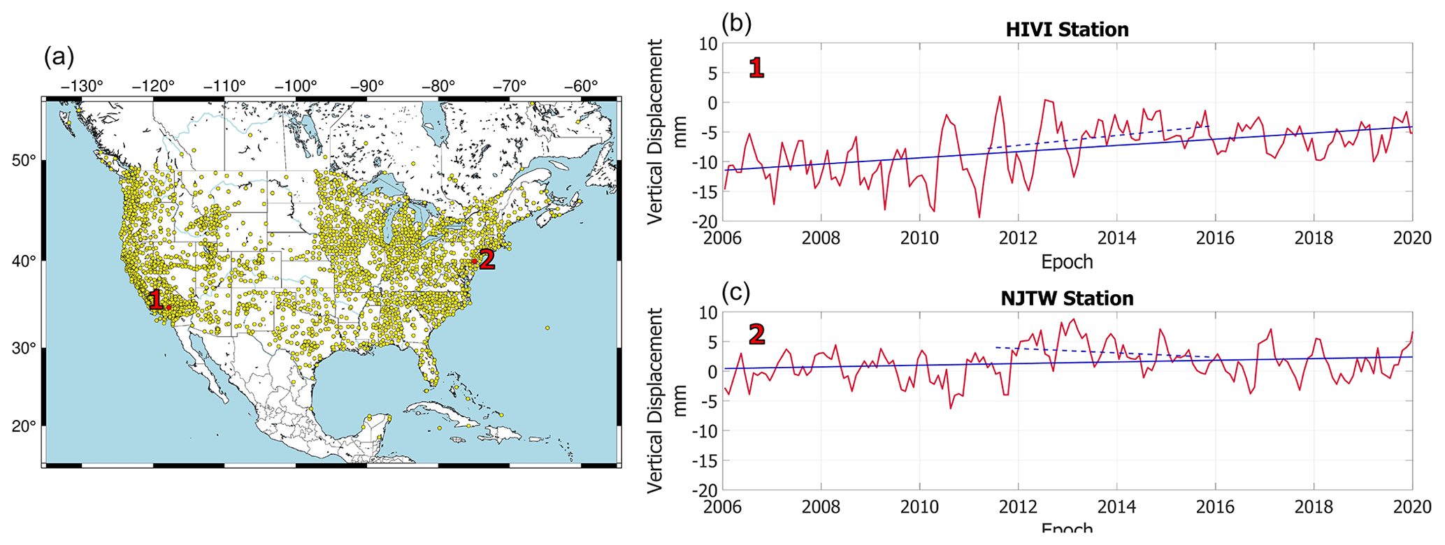
Figure 1(a) Map of the study area. GPS stations are shown in yellow; (b) vertical displacement time series of two random stations (red line). The solid blue line denotes the overall trend of the time series and the dashed blue line the trend between May 2011 and May 2015. Note the significant uplift of the HIVI station located in southern California.
2.2 External validation datasets – time-variable gravity field
We compare GPS observations of vertical displacement against GRACE(-FO) estimates of solid Earth's elastic vertical displacement from terrestrial water, snow, and ice.
To compare to GRACE(-FO), we analyze JPL's 3° mascon solution (Release 6, Watkins et al., 2015; Wiese et al., 2016). The effect of glacial isostatic adjustment is removed from GRACE(-FO) products using ICE-6G_D model estimates (Peltier et al., 2018). The geocenter motion (degree 1) coefficient is using the technique of Sun et al. (2016) (Technical Note 13). Values of C20 (Earth's oblateness) and C30 (for months after August 2016) are substituted with SLR data (Loomis et al., 2019). We calculate solid Earth's elastic response by using the loading Love number of the Preliminary Reference Earth Model (Wang et al., 2012).
Estimates of GPS positions in ITRF2014 (Altamimi et al., 2016) are relative to the center of mass (CM) in the long term but relative to the center of the figure (CF) in the seasons (because ITRF2014 does not allow seasonal oscillations of CM). We therefore remove the long-term rate of CM relative to CF to transform the GRACE estimates in the long term from CF to CM (but do not remove seasonal oscillations of CM relative to CF so as to preserve the ITRF seasonal frame relative to CF). The annual signal of the geocenter (as realized by ITRF 2014) projected on the up component in North America on average explains 3 % of the GPS vertical displacement signal and can explain up to 20 % for certain sites.
GRACE(-FO) vertical displacement monthly estimates are derived as follows (e.g., Davis et al., 2004):
where U is the estimate of vertical displacement; a denotes the Earth's radius; ϕ and λ denote the latitude and longitude, respectively; Plm represents the associated Legendre polynomials; and are the elastic gravity and vertical load Love numbers (Wang et al., 2012), respectively; and C and S are the spherical harmonic coefficients derived from GRACE(-FO) monthly solutions with respect to degree l and order m. JPL releases gridded mascon fields to derive spherical harmonics (C and S in Eq. 1). We transform fields of equivalent water height to normalized harmonic coefficients using the inverse of Eq. (9) in Wahr et al. (1998). Like GPS, we subtract the GRACE(-FO) vertical displacement field of September 2012 from each monthly field to establish a common reference basis. GRACE(-FO) fields are estimated at a 0.5° spatial resolution (ϕλ in Eq. 1). Thus, we extract GRACE(-FO) estimates at the station level by bilinearly interpolating the vertical displacement from the nearest 0.5° grid-point neighbors to the station's location.
2.3 Screening metrics
GPS vertical displacement estimates are evaluated against the ones derived from GRACE(-FO) to assist in identifying outliers or further corrections that may be needed. We employ a number of different metrics to evaluate the agreement between the two datasets and to determine whether to include it in the joint solution or not. Similar to Yin et al. (2020) we quantify correlation and variance reduction between GPS and GRACE(-FO) vertical displacements. The structure of surface mass periodic signals (e.g., annual cycles, trends) as picked up by the two measurement techniques also entails critical information regarding mis-modeled offsets and is evaluated as well.
This process flags sites that need correction and corroborates joint inversion's hypothesis (Argus et al., 2021) that a basic level of agreement is needed for the GPS data to be used to infer surface mass change.
2.3.1 Correlation
First, we specify the level of agreement between the datasets by estimating the Pearson correlation coefficient between GPS and GRACE(-FO) time series. On average correlation is 62 %, but stations located on the west coast exhibit agreement higher than 80 %, which in most cases is driven by the larger annual signal amplitude there. A more detailed look into the correlation metric is performed to evaluate the agreement of GPS/GRACE(-FO) in retrieving the seasonal cycle amplitude in different watersheds. We fit and remove a trajectory model y(t):
with a being the intercept, b being the trend, and A and B being the amplitudes of the sine and cosine components of a periodic function. In a future release of the dataset, we will evaluate the presence of draconitic periods in the time series and add them to the trajectory model if justified. With the time span of the current time series being up to 15 years, we cannot resolve for the draconitics (i.e., the first draconitic period of 351.6 d and the annual cycle of 365.25 d are very close and require a long time series to be deciphered). For a more thorough discussion we refer the interested reader to Amiri-Simkooei et al. (2017) and Klos et al. (2023).
We classify stations in watersheds and plot the GPS–GRACE(-FO) correlation coefficient (R) of each station in different watershed against the amplitude of annual signals (Fig. 2b). To quantify the relationship between the magnitude of the annual cycle and correlation between the two datasets we fit a linear function between the magnitude of the annual signals and the GPS–GRACE(-FO) vertical displacement correlations for each watershed separately. A steep slope (a) of the fit (a>0.5) indicates agreement between the two datasets, which depends on the magnitude of the annual cycle. This relationship breaks when stations of a basin exhibit smaller annual cycles. We discuss an interesting case in the Supplement, where stations located in the Great Lakes region (part of the St. Lawrence watershed) demonstrate a negative trend if . The disagreement is even more pronounced when assessing the second metric (i.e., trends). Both metrics, when taken together, helped us identify the source problem (i.e., unlogged offset that affected nearly 25 % of the stations located in the St. Lawrence watershed) and take corrective actions (see the Supplement for more details). Note that for Figs. 2 and 3 the corrected data were used.
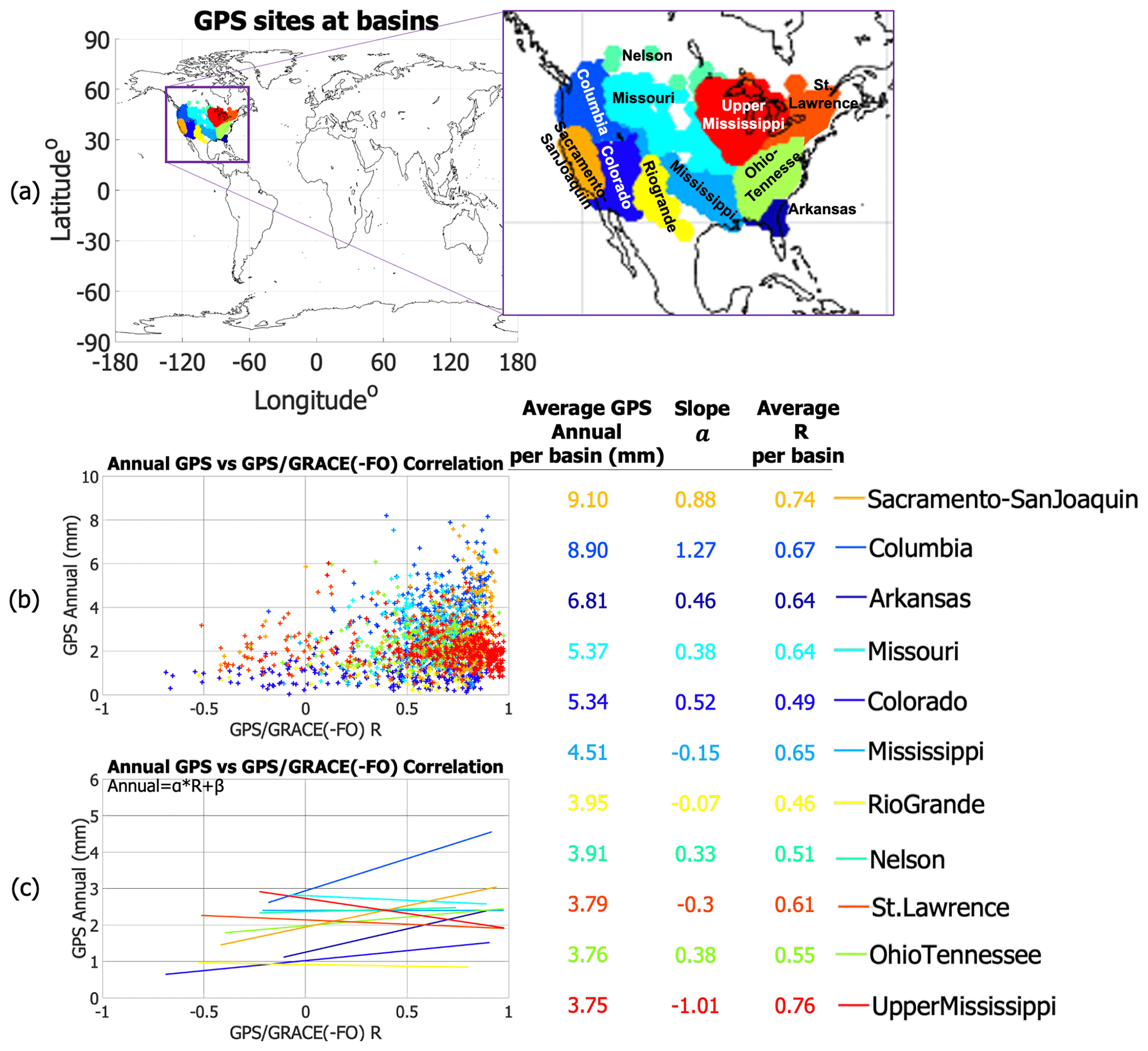
Figure 2(a) GPS site clusters at watersheds in the US. Each watershed has a different color; (b) magnitude of annual GPS vertical displacement cycles derived with respect to GPS–GRACE(-FO) correlation; (c) linear fit between the magnitude of the annual GPS vertical displacement cycles and GPS–GRACE(-FO) correlation.
2.3.2 Trends
In order to study the agreement between GPS and GRACE(-FO) in more detail, we split the time series of each station into non-overlapping intervals of 36 months and fit Eq. (2) for each station during each time window. Different time lengths of the GPS series may lead to misinterpretation of the geophysical content. For example, a station that has records only for the first 13 months out of the total 36-month window may reflect different fit constituents compared to a neighbor station with full records if the actual behavior of Earth's response changes during the 36-month window. Although in our dataset this case is rare, we proceed with deriving the rate (slope) and the annual cycles only for stations that have records for at least 28 out of the 36 months. We did not interpolate the series during the GRACE(-FO) gap; thus, the last time window reflects trends estimated using only GRACE-FO and GPS time series between June 2018 and 2021. As expected, GPS rates feature higher spatial variability than GRACE(-FO). However, both techniques capture large-scale quasi-periodic variations every 3 years (Fig. 3), agreement that is noteworthy. The effect of this metric to detect outliers is pronounced when the two techniques show flipped trends.
Regions with pronounced trend disagreement include the following.
-
St. Lawrence watershed (stations located in the Great Lakes region in the state of Michigan). The trend during 2015–2018 was flipped between GPS and GRACE(-FO) at 62 stations (St. Lawrence watershed has a total of 243 stations available between 2015 and 2018). We discovered a missed offset in the series occurring in April 2016 and corrected for it, which led to improved agreement in the trend (see the Supplement).
-
Cascadia region (northwest coast). The disagreement is evident in maps spanning 2009–2012, 2015–2018, and 2018–May 2021. GPS sites record a large surface uplift, which over the course of 15 years sums to 60 mm at sites located on Vancouver Island. GRACE(-FO) does not capture any such behavior. We attribute this disagreement partly to (1) glacial isostatic adjustment modeling error, which manifests oppositely with the two techniques. ICE6G_D predicts too much subsidence, and thus when we correct GPS, we find too much uplift and when we correct GRACE(-FO) we find too much water gain which predicts too much subsidence. The disagreement is also partly attributed to (2) the interseismic strain accumulation correction applied in the GPS dataset over this area (Argus et al., 2021). The sites have been flagged and are not going to be used in the joint inversion.
-
San Andreas Fault (southern California). Sites located in the vicinity of the Parkfield segment of the fault (Carrizon plain) exhibit consistent disagreement in the trend. More investigation is required to understand the mechanism that the fault presents in GPS/GRACE(-FO) vertical displacement estimates. The disagreement is also seen in Argus et al. (2022, Fig. S12). The sites have been flagged and are not going to be used in the joint inversion.
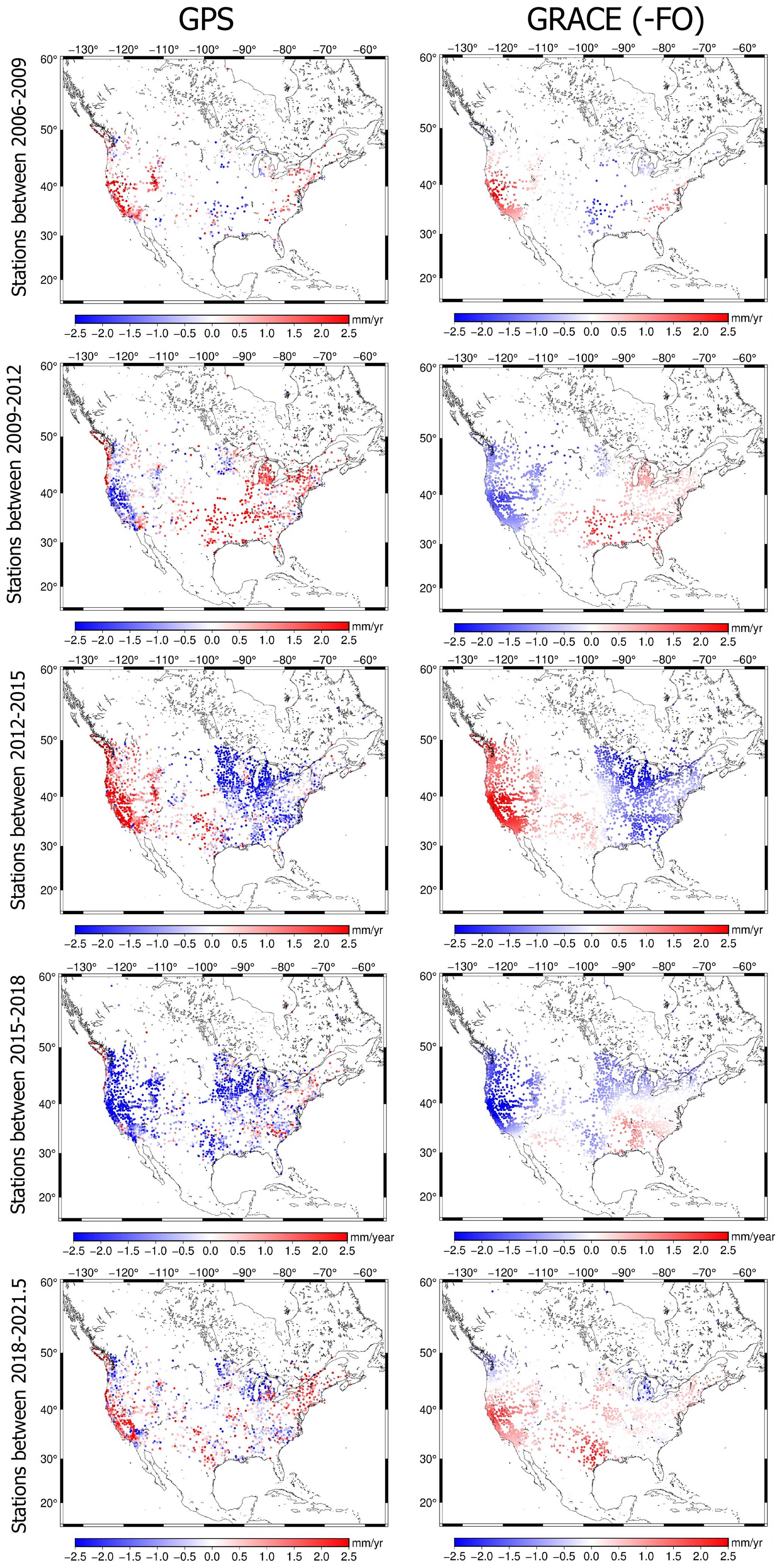
Figure 3Rates of vertical displacements derived by GPS and GRACE. The rates are calculated every 36 months (3 years) between 2006 and 2021.
2.3.3 Variance reduction
Similarity in both amplitude and phase between two quantities is quantified via the variance attenuation factor (Gaspar and Wunsch, 1989; Fukumori et al., 2015).
The higher the agreement in phase and amplitude between GPS and GRACE(-FO), the closer the metric gets to 100 %. varred may also be negative when the differences in amplitude and/or phase are large. Overall, GPS and GRACE(-FO) are consistent when varred exceeds 50 %. The areas of main disagreement are near coasts, especially along the Atlantic Ocean. This inconsistency can be partly explained by modeling errors of the non-tidal oceanic and atmospheric loading model (e.g., Klos et al., 2021; van Dam et al., 2007). Additionally, agreement is poor for sites located in the vicinity of the Parkfield segment (specific regions across the fault perform poorly), which is consistent with the disagreement shown in Fig. 3.
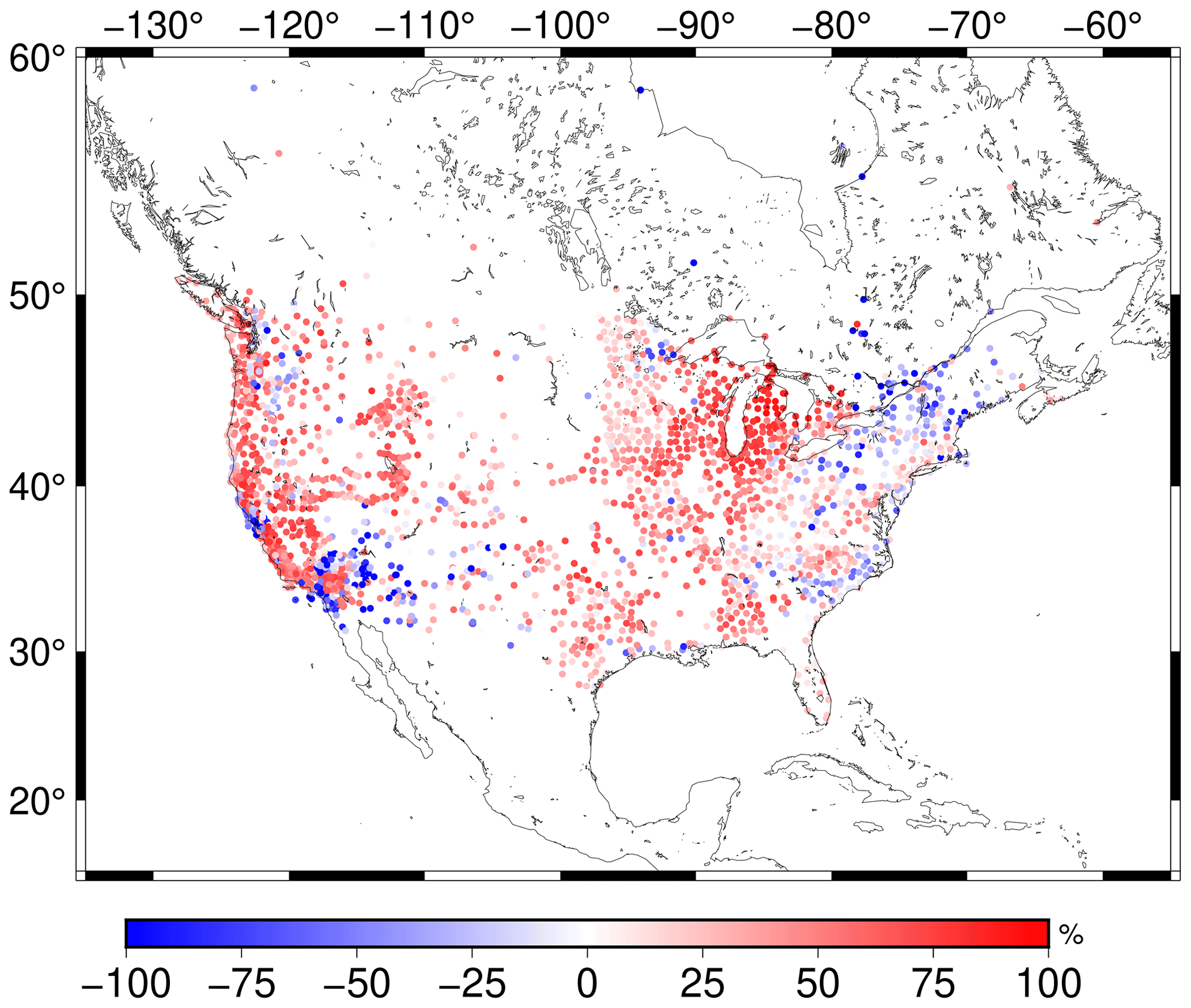
Figure 4Variance reduction between GPS and GRACE(-FO) vertical displacements.
We also compared the annual amplitudes of GPS and GRACE(-FO) vertical displacements (cosine and sine components in Eq. 2). This analysis was not informative for the presence of outliers or errors in the current data sample studied.
Overall, the screening process not only assisted in outlier detection, but it also allowed for a deeper look into the structure of vertical displacement periodic signals. We identified the need for antenna offset corrections (in sites located in the Great Lakes region); removed sites affected by glacial isostatic adjustment and interseismic modeling errors; and sites located at the Parkfield segment of San Andreas Fault.
With the updated dataset we are now ready to proceed with the uncertainty quantification of the GPS vertical displacement time series. We apply different error characterization schemes consisting of a root sum square of a random error, white noise error, power-law noise error (flicker noise and random walk), and spatially coherent error.
3.1 Methods
3.1.1 Root mean square error
Residuals r of a series with respect to a trajectory model (Eq. 2) are often used as a first approximation of noise in vertical displacement series (e.g., Bos et al., 2013; Michel et al., 2021). Practically, r shows how well a trajectory model can describe the original time series. Therefore, the root mean square (rms) of r can give a first approximation of the noise floor of each station.
3.1.2 Spectral analysis, white, flicker, and random walk noise
The power distribution of residuals (and its agreement with noise models) is another popular way to quantify uncertainty of GPS time series (e.g., Klos et al., 2019; Argus et al., 2022). Typically, GPS series are evaluated for white, flicker, and random walk noise or a combination of them. Hector software (Bos et al., 2013) is used to estimate full noise covariance information by means of a maximum likelihood estimator. The covariance matrix C from a combination of white and power-law (i.e., flicker and random walk) noise is given as
where a is the amplitude of white noise, I is the identity matrix of size N (number of samples and/or epochs in the series), b is the amplitude, and J is the covariance matrix of power-law noise. The J matrix is a full covariance matrix that describes the time-correlated error (as the data record length increases, the displacement uncertainty changes; Bos et al., 2008, Eqs. 8–11). The optimal selection of the noise models is done via two optimality criteria, namely the Akaike information criterion (Akaike, 1974) and the Bayesian criterion (Schwarz, 1978).
In this study, we consider three cases:
- a.
white noise (WN),
- b.
a combination of WN and flicker noise (WN+FN), and
- c.
a combination of WN, FN, and random walk noise (WN+FN+RW).
We take the root sum squares of the noise magnitudes as our noise floor. For example, for the case of WN+FN noise, noise is derived as . Our data are sampled on a monthly basis, and thus σFN needs to be scaled appropriately, i.e., , where, σPL is the uncertainty of the power law (PL) and k the spectral index outputted from Hector (more information on power-law noise estimation can be found in Bos et al., 2008, and Williams, 2003).
3.1.3 Common mode noise
The common mode component (CMC) is derived following the processing scheme suggested by Kreemer and Blewitt (2021), which can be summarized as follows.
-
Input GPS displacement time series (referenced to September 2012) for j stations (lj).
-
Derive each station's residuals by removing the trajectory part of the series (lj(t)−yj(t)).
-
Quantify the correlation coefficient rMAD using robust statistics. rMAD is defined as
The median absolute deviation (MAD) is the absolute deviation around the median. For example, for a residual series res(t) MAD . u and v are derived as
with p and q being the residual series of the reference station and the neighbor station, respectively. For each station there are j−1 correlation coefficients rMAD. In order to decide the cut-off distance for which a neighbor station will be considered in the analysis we plot the rMAD coefficient against its distance from the reference station (Fig. 5). Based on results from all stations we decide to set a cut-off at 1500 km, slightly higher than the 1350 km suggested by Kreemer and Blewitt (2021). The 1500 km cut-off allows us to separate stations between the east and west coast, as spatially coherent signals at stations located across the continent are negligible.
-
Derive the median slope estimator (ccs) using the Theil–Sen median trend. The ccs is the median trend of the rMAD coefficients of a station against their distance with the reference station.
-
Derive the zero-distance intercept ccij for each station as , with d being the distance between the station of reference and the neighbor station (maximum d=1500 km).
-
Construct CMC: calculate the cumulative (cj) and percentile (pj) weights for each station and then find the weighted median that corresponds to pj=50 %. This weighted median represents the CMC of the station (Fig. 6).
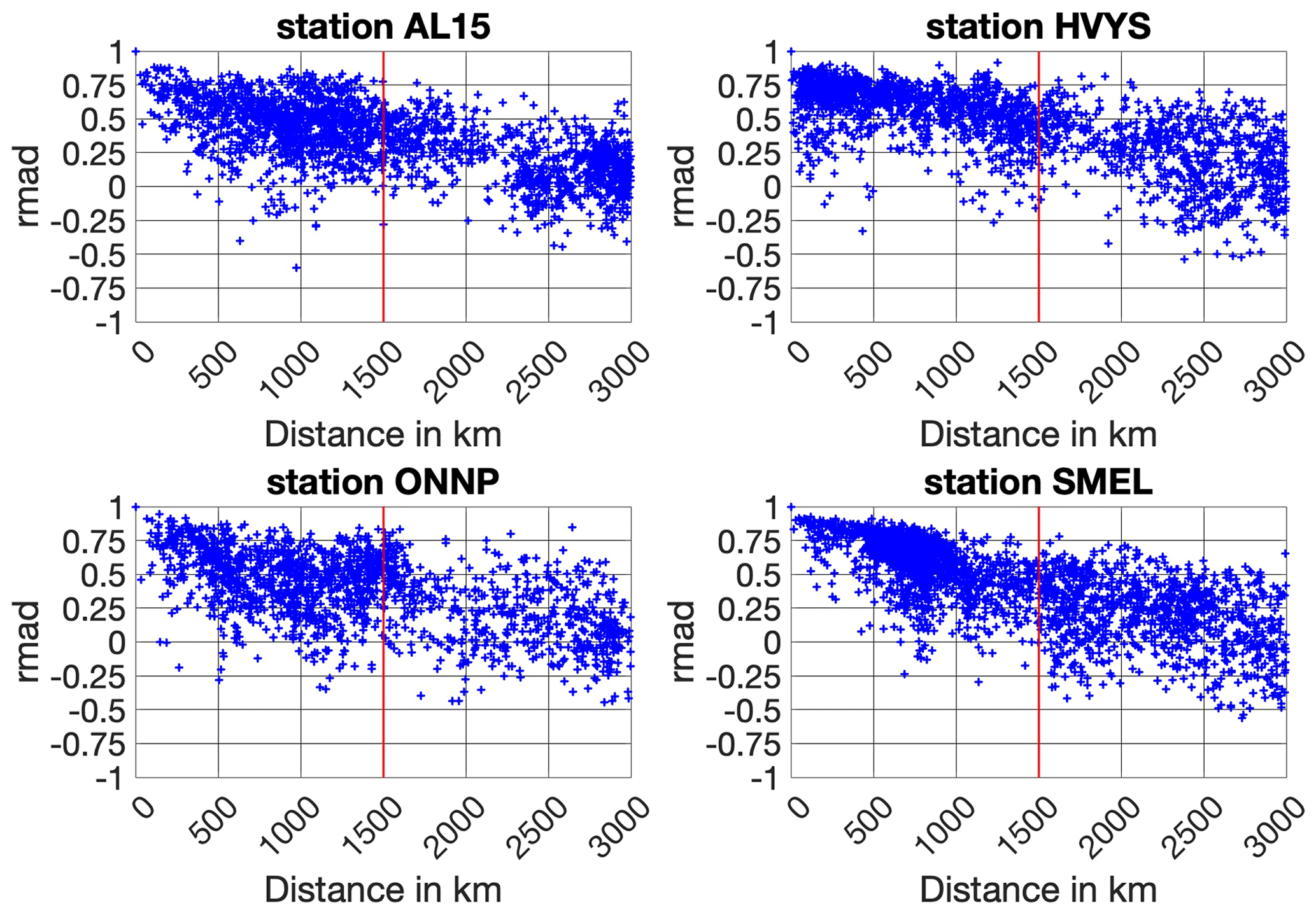
Figure 5rMAD coefficient of four random stations with the rest of the station sample, plotted against the distance of the reference station with the rest of the stations. Each cross resembles the rMAD of the reference station with a station located at distance d.
CMC is limited in providing a realistic error approximation in that the technique cannot isolate spatially correlated noise from signal (e.g., hydrology signals not described by the trajectory model are present in the residuals fed into CMC). Under the realistic assumption that a component of the high-frequency signal contained in CMC reflects real hydrological processes, we remove the contribution of surface hydrology using Global Land Data Assimilation System (GLDAS) (Rodell et al., 2004) vertical displacement estimates. GLDAS does not model deep groundwater and open surface water, so these signals remain in the residual (Scanlon et al., 2018). Vertical displacement estimates driven by surface hydrology are derived similarly to GRACE(-FO) (Sect. 2.2). We use Noah v2.1 monthly estimates of soil moisture storage given at 0.25° grids (Beaudoing and Rodell, 2020), convert the fields from terrestrial water storage (kg m−2) to units of equivalent water height, derive the spherical harmonic coefficients of the equivalent water height mass load using Wahr et al. (1998), and predict the elastic response of the Earth (Eq. 1). Afterwards, we remove the reference epoch (September 2012) similar to GPS and estimate the vertical displacement at the locations of the GPS sites by interpolating the estimates of the closest neighbors to the station's location. Note that because our interest is to prepare the data for a combined solution with GRACE(-FO) we interpolate the time series at the times of GRACE(-FO) monthly series availability. The interested reader is referred to the Supplement, where we show the vertical displacement estimated by GPS, GRACE(-FO), and GLDAS (Fig. S2) for randomly selected stations. Finally, we derive residuals relative to the trajectory model (Eq. 2). GLDAS (surface hydrology) residuals should ideally reflect high-frequency hydrological processes and are therefore removed from GPS residuals. Overall, CMC of surface hydrology residuals exhibits a fairly small magnitude (∼ 0.5 mm). We remove the contribution of surface hydrology within the CMC algorithm by first subtracting GLDAS vertical displacement estimates from GPS and next inputting the residuals of this difference into the algorithm. The output of this process (CMCHF) slightly decreases the magnitude of CMC and expresses a more realistic representation of spatially correlated noise.
3.2 Results
Vertical displacement uncertainty of each station is estimated by means of all the different approaches discussed in Sect. 3. Mean (μ), median, and standard deviation (SD) values are shown in Table 1. On average, an assumption of white noise shows slightly reduced uncertainty compared to the other techniques, followed by RMSE. When flicker noise is considered in addition to white noise (WN+FN) the average uncertainty increases by nearly 0.8 mm compared to the white noise only. We note that the contribution of white noise in the case of WN+FN is negligible for 97 % of the stations (that is, flicker noise describes the noise exclusively). Noise level from the combination of all three noise models (WN+FN+RW) is less than 4 mm on average. In this case too, white noise is negligible, and noise is described exclusively from flicker noise for 1550 stations and from random walk for 600 stations. The rest of the data sample reflects a contribution from both noise models. We additionally analyzed the amplitude of the noise of each noise model (σPL) with respect to the length of the input series. Results did not identify any clear relationship between σPL and the length of each station's time series. The CMC noise floor is 3.6 mm on average with a relatively large standard deviation (±1.6 mm), which suggests that spatially correlated noise has higher variability than time-correlated noise (±1.6 mm as opposed to ∼ ±1 mm). When surface hydrology is removed (CMCHF) the noise floor drops by a fraction of a millimeter on average compared to CMC.
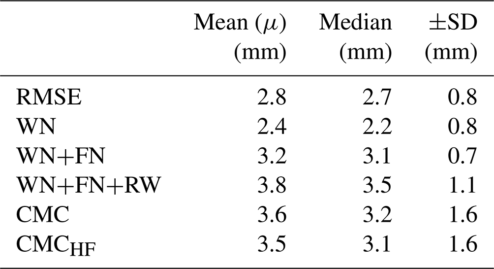
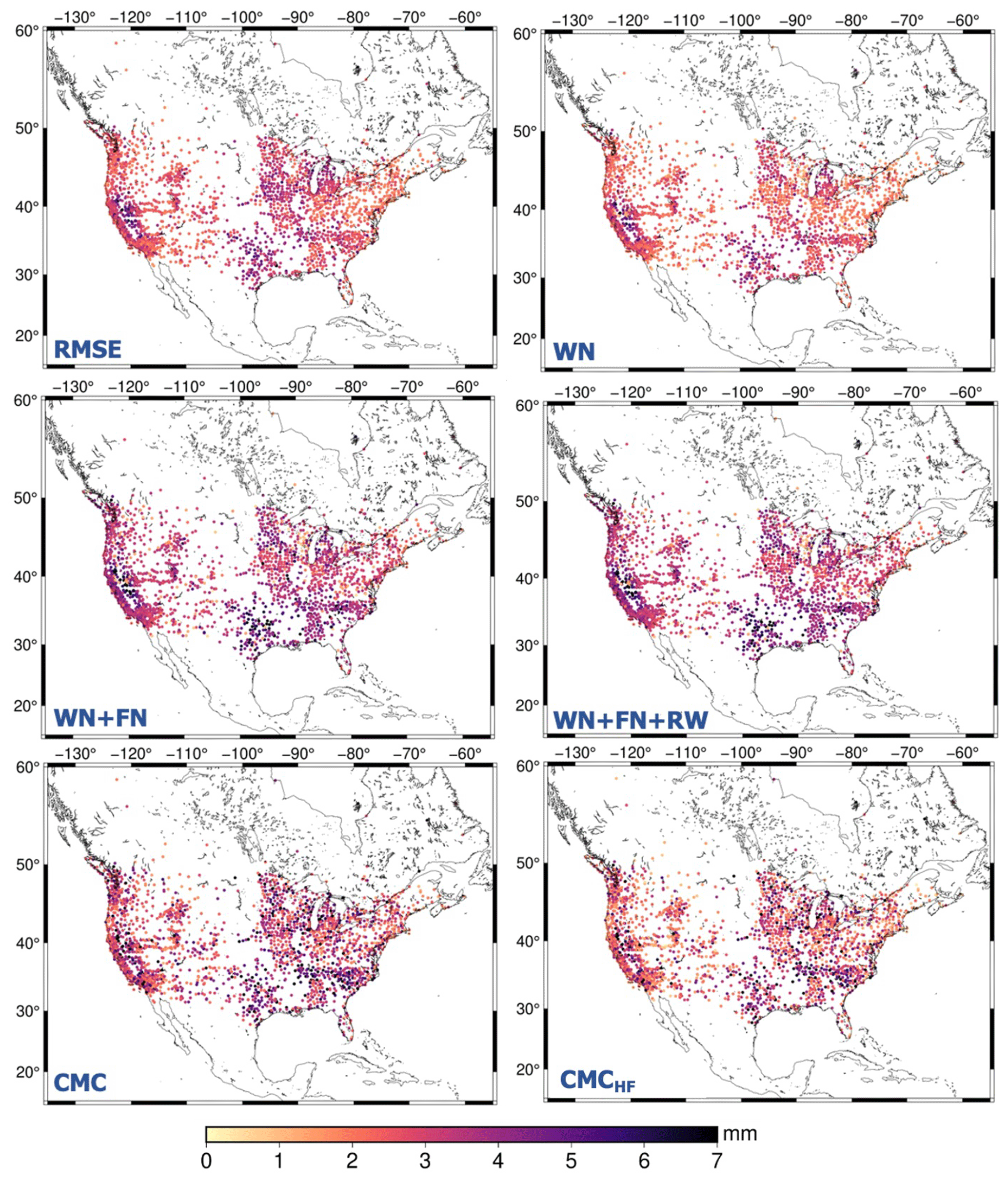
Figure 6Noise amplitudes of GPS time series estimated using different techniques.
RMSE and WN exhibit a smooth transition among the regions, which indicates the presence of a spatially coherent regime signal mostly driven by hydrology (Fig. 6). The combination of WN+FN is mostly dominated by FN, and the uncertainty exhibits local (in space) coherence. The uncertainty is larger when random walk is included in the combination (WN+FN+RW). A recent study from Argus et al. (2022) on groundwater flux in Central Valley (California) suggests that noise on GPS-derived uplift motion can be well described by a combination of flicker noise and random walk due to the ability of these noise models to reflect low-frequency noise. When a simulated contribution of the surface hydrological component is removed from the series, CMCHF reflects a more realistic picture of the noise. Arguably the level of change compared to CMC is sub-millimeter. Signal contributions from un-modeled groundwater variations are potentially still present, but groundwater changes are typically slower in time.
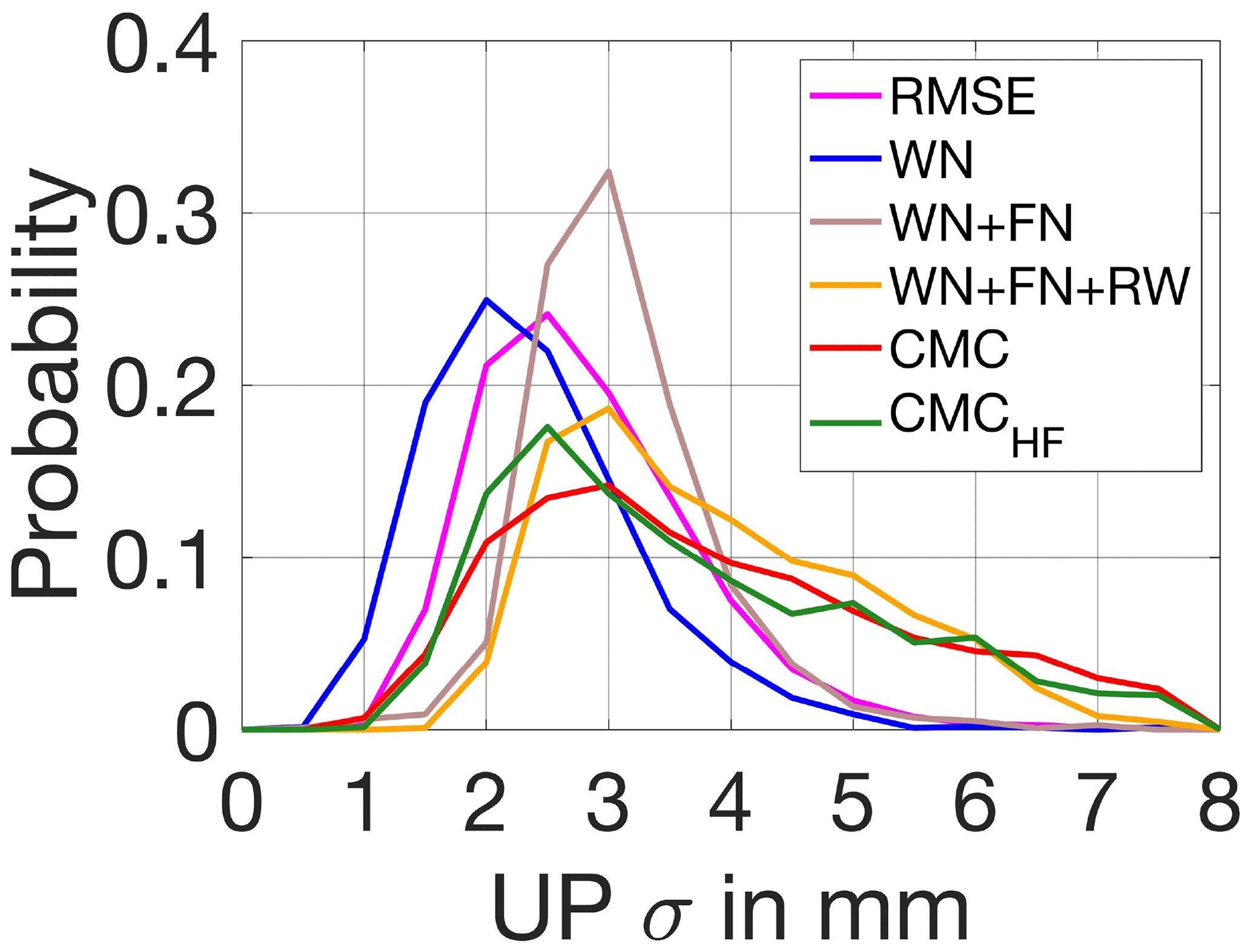
We obtain the relative likelihood of each uncertainty quantification method by estimating the probability density function (PDF) (Fig. 7). White noise has a flat power spectrum, having the same amplitude across frequencies. Estimating a best fit for a flat spectrum does not allow for capturing the long tail skew of the residuals (low frequency), which are biased towards their mean. Thus, the amplitude of white noise is smaller compared to the rest of the techniques (Table 1). Flicker and random walk noise models add to the long tail of the power distribution: that is, they allow more low-frequency noise, which explains the higher amplitude of the uncertainty when these two noise types are considered.
RMSE and WN show a 50 % probability of a station having an uncertainty (σ) between 1.5 and 2 mm and less than a 10 % probability of a station exceeding σ=4 mm. The noise level fells within [2 4] mm for ∼ 93 % of the stations when we consider combination of WN+FN. PDFs of RMSE, WN, and WN+FN resemble a normal distribution, with the mean being shifted for each case. When random walk is also considered (WN+FN+RW) 64 % of the stations exhibit noise within [2 4] mm. In this case, the distribution is more spread, resembling a gamma-like distribution, with a peak being at 3 mm (18 %). CMC and CMCHF PDFs also follow a gamma shape, and the probability of the uncertainty ranging [2 4] mm is nearly 60 % for CMC and 65 % when surface hydrology is removed.
The data product described in the paper is available on Zenodo (DOI: https://doi.org/10.5281/zenodo.8184285, Peidou et al., 2023). GPS time series are provided by the Global Station List from the Nevada Geodetic Laboratory (http://geodesy.unr.edu/, last access: 28 January 2024, Blewitt et al., 2018). The non-atmospheric and oceanic tidal aliasing product (AOD1B RL06) is provided by GFZ's Information System and Data Center (ftp://isdc.gfz-potsdam.de/grace/Level-1B/GFZ/AOD/RL06, last access: 28 January 2024, Dobslaw et al., 2017). GRACE-FO Level 2 products are available from PODAAC (https://doi.org/10.5067/GFL20-MJ060, NASA JPL, 2019).
GPS-derived vertical displacements are very useful for supplementing GRACE(-FO) gravity products to infer mass change signals at spatial scales smaller than what can typically be achieved with current satellite gravimetry alone (i.e., < 300 km). This work provides a general workflow to isolate elastic surface mass signals from GPS vertical displacement by developing processing standards; additionally, it suggests uncertainty quantification schemes to quantify error in GPS vertical displacement estimates. The ultimate goal is to prepare GPS estimates for merging with satellite gravimetry observations. First, we provide a list of corrections needed for isolating surface mass following recommendations outlined in Argus et al. (2017, 2022). Additionally, a detailed investigation of trends, correlation, and variance reduction highlights the need for better background modeling (glacial isostatic adjustment and interseismic strain), as the two observation techniques respond differently in the presence of such errors. At this point the recommendation is to remove sites located in the vicinity of regions where background models are known to perform poorly, before any joint inversion. Except detecting outlier stations, screening metrics point to extra corrections that need to be applied in certain sites (e.g., missed antenna offsets).
Several uncertainty quantification schemes have been tested to prescribe weights on GPS vertical displacement estimates that are needed for a joint inversion with GRACE(-FO) data. The average noise level indicated by RMSE is 2.8 mm. White noise average is 2.5 mm. The errors increase when lower frequencies are included in the noise estimation. When we account for flicker noise, one-third of the sites exhibit noise levels of up to 3 mm. The average noise increases significantly in the presence of random walk, as more power of the lower frequencies gets into the estimations, and the distribution of noise is more dispersed. In this case, half of the stations are prescribed with > 4 mm uncertainty. Argus et al. (2022) find that random walk is the most realistic representation of noise based on post-fit residuals. We notice that the spectrum of CMC provides similar uncertainties to random walk, which implies that despite the different characterization procedure, CMC is able to provide equally realistic noise estimates of GPS time series. We attempted to minimize lingering hydrology signals embedded in CMC by reducing the GPS vertical displacement observations with displacements from the GLDAS hydrology model. The average noise floor dropped slightly (∼ 0.5 mm drop in sigma). Future work will provide further information on GPS station errors when the weight of each GPS site is also considered based on its impact on the performance in a formal data combination of GPS and GRACE(-FO). The suggested framework can be easily adjusted to account for global datasets. The new dataset provides GPS vertical displacements of elastic mass variations in North America and their associated uncertainties.
The supplement related to this article is available online at: https://doi.org/10.5194/essd-16-1317-2024-supplement.
AP outlined the methodology, performed the analysis, and wrote the paper. DFA processed the GPS time series and outlined the methodology to isolate surface mass loading from GPS time series. FWL and DNW helped with the GPS and GRACE(-FO) data screening and provided critical feedback and ideas. ME helped with the uncertainty quantification schemes. All authors reviewed and substantially edited the paper.
The contact author has declared that none of the authors has any competing interests.
Publisher's note: Copernicus Publications remains neutral with regard to jurisdictional claims made in the text, published maps, institutional affiliations, or any other geographical representation in this paper. While Copernicus Publications makes every effort to include appropriate place names, the final responsibility lies with the authors.
Maps were made with the Generic Mapping Toolbox (Wessel et al., 2019). We thank Corne Kreemer (UNR) for his feedback and Mike Heflin (JPL) for his insights on draconitic errors.
This research was carried out at the Jet Propulsion Laboratory, California Institute of Technology, under a contract with the National Aeronautics and Space Administration (NASA; grant no. 80NM0018D0004) with support from the GRACE-FO Science Team grant (80NM0018F0585).
This paper was edited by Kirsten Elger and reviewed by two anonymous referees.
Akaike, H.: A new look at the statistical model identification, IEEE T. Automat. Contr., 19, 716–723, https://doi.org/10.1109/TAC.1974.1100705, 1974.
Altamimi, Z., Rebischung, P., Métivier, L., and Collilieux, X.: ITRF2014: A new release of the International Terrestrial Reference Frame modeling nonlinear station motions, J. Geophys. Res.-Sol. Ea., 121, 6109–6131, https://doi.org/10.1002/2016JB013098, 2016.
Amiri‐Simkooei, A. R.: On the nature of GPS draconitic year periodic pattern in multivariate position time series, J. Geophys. Res.-Sol. Ea., 118, 2500–2511, 2013.
Amiri-Simkooei, A. R., Mohammadloo, T. H., and Argus, D. F: Multivariate analysis of GPS position timeseries of JPL second reprocessing campaign, J. Geodesy, 91, 685–704, https://doi.org/10.1007/s00190-016-0991-9, 2017.
Argus, D. F. and Peltier, W. R.: Constraining models of postglacial rebound using space geodesy: a detailed assessment of model ICE-5G (VM2) and its relatives, Geophys. J. Int., 181, 697–723, https://doi.org/10.1111/j.1365-246X.2010.04562.x, 2010.
Argus, D. F., Gordon, R. G., Heflin, M. B., Ma, C., Eanes, R. J., Willis, P., Peltier, W. R., and Owen, S. E.: The angular velocities of the plates and the velocity of Earth's centre from space geodesy, Geophys. J. Int., 180, 913–960, https://doi.org/10.1111/j.1365-246X.2009.04463.x, 2010.
Argus, D. F., Fu, Y., and Landerer, F. W.: Seasonal variation in total water storage in California inferred from GPS observations of vertical land motion, Geophys. Res. Lett., 41, 1971–1980, https://doi.org/10.1002/2014GL059570, 2014a.
Argus, D. F., Peltier, W. R., Drummond, R., and Moore, A. W.: The Antarctica component of postglacial rebound model ICE-6G_C (VM5a) based on GPS positioning, exposure age dating of ice thicknesses, and relative sea level histories, Geophys. J. Int., 198, 537–563, https://doi.org/10.1093/gji/ggu140, 2014b.
Argus, D. F., Landerer, F. W., Wiese, D. N., Martens, H. R., Fu, Y., Famiglietti, J. S., Thomas, B. F., Farr, T. G., Moore, A. W., and Watkins, M. M.: Sustained water loss in California's mountain ranges during severe drought from 2012 to 2015 inferred from GPS, J. Geophys. Res.-Sol. Ea., 122, 10–559, https://doi.org/10.1002/2017JB014424, 2017.
Argus, D. F., Peltier, W. R., Blewitt, G., and Kreemer, C.: The Viscosity of the Top Third of the Lower Mantle Estimated Using GPS, GRACE, and Relative Sea Level Measurements of Glacial Isostatic Adjustment, J. Geophys. Res.-Sol. Ea., 126, 2020JB021537, https://doi.org/10.1029/2020JB021537, 2021.
Argus, D. F., Martens, H. R., Borsa, A. A., Knappe, E., Wiese, D. N., Alam, S., Anderson, M., Khatiwada, A., Lau, N., Peidou, A., and Swarr, M.: Subsurface water flux in California's Central Valley and its source watershed from space geodesy, Geophys. Res. Lett., 49, e2022GL099583, https://doi.org/10.1029/2022GL099583, 2022.
Beaudoing, H. and Rodell, M.: GLDAS Noah Land Surface Model L4 monthly 0.25 x 0.25 degree V2.1, Greenbelt, Maryland, USA, Goddard Earth Sciences Data and Information Services Center (GES DISC) [data set], https://doi.org/10.5067/SXAVCZFAQLNO, 2020.
Becker, J. M. and Bevis, M.: Love's problem, Geophys. J. Int., 156, 171–178, https://doi.org/10.1111/j.1365-246X.2003.02150.x, 2004.
Bertiger, W., Bar-Sever, Y., Dorsey, A., Haines, B., Harvey, N., Hemberger, D., Heflin, M., Lu, W., Miller, M., Moore, A. W., and Murphy, D.: GipsyX/RTGx, a new tool set for space geodetic operations and research, Adv. Space Res., 66, 469–489, https://doi.org/10.1016/j.asr.2020.04.015, 2020.
Bevis, M. and Brown, A.: Trajectory models and reference frames for crustal motion geodesy, J. Geodesy, 88, 283–311, https://doi.org/10.1007/s00190-013-0685-5, 2014.
Blewitt, G., Lavallée, D., Clarke, P., and Nurutdinov, K.: A new global mode of Earth deformation: Seasonal cycle detected, Science, 294, 2342–2345, https://doi.org/10.1126/science.1065328, 2001.
Blewitt, G., Hammond, W. C., and Kreemer, C.: Harnessing the GPS data explosion for interdisciplinary science, Eos, 99, p. 485, https://doi.org/10.1029/2018EO104623, 2018.
Boehm, J., Werl, B., and Schuh, H.: Troposphere mapping functions for GPS and very long baseline interferometry from European Centre for Medium-Range Weather Forecasts operational analysis data, J. Geophys. Res., 111, B02406, https://doi.org/10.1029/2005JB003629, 2006.
Bos, M. S., Fernandes, R. M. S., Williams, S. D. P., and Bastos, L.: Fast error analysis of continuous GPS observations, J. Geodesy, 82, 157–166, https://doi.org/10.1007/s00190-007-0165-x, 2008.
Bos, M. S., Fernandes, R. M. S., Williams, S. D. P., and Bastos, L.: Fast error analysis of continuous GPS observations with missing data, J. Geodesy, 87, 351–360, https://doi.org/10.1007/s00190-012-0605-0, 2013.
Chew, C. C. and Small, E. E.: Terrestrial water storage response to the 2012 drought estimated from GPS vertical position anomalies, Geophys. Res. Lett., 41, 6145–6151, https://doi.org/10.1002/2014GL061206, 2014.
Crowell, B. W., Bock, Y., and Liu, Z.: Single-station automated detection of transient deformation in GPS timeseries with the relative strength index: A case study of Cascadian slow slip, J. Geophys. Res.-Sol. Ea., 121, 9077–9094, https://doi.org/10.1002/2016JB013542, 2016.
Davis, J. L., Elósegui, P., Mitrovica, J. X., and Tamisiea, M. E.: Climate-driven deformation of the solid Earth from GRACE and GPS. Geophys. Res. Lett., 31, L24605, https://doi.org/10.1029/2004GL021435, 2004.
Dill, R. and Dobslaw, H.: Numerical simulations of global-scale high resolution hydrological crustal deformations, J. Geophys. Res.-Sol. Ea., 118, 5008–5017, https://doi.org/10.1002/jgrb.50353, 2013.
Dobslaw, H., Bergmann-Wolf, I., Dill, R., Poropat, L., Thomas, M., Dahle, C., Esselborn, S., König, R., and Flechtner, F.: A new high-resolution model of non-tidal atmosphere and ocean mass variability for de-aliasing of satellite gravity observations: AOD1B RL06, Geophys. J. Int., 211, 263–269, https://doi.org/10.1093/gji/ggx302, 2017.
Dong, D., Fang, P., Bock, Y., Webb, F., Prawirodirdjo, L., Kedar, S., and Jamason, P.: Spatiotemporal filtering using principal component analysis and Karhunen-Loeve expansion approaches for regional GPS network analysis, J. Geophys. Res., 111, B03405, https://doi.org/10.1029/2005JB003806, 2006.
Frederikse, T., Landerer, F., Caron, L., Adhikari, S., Parkes, D., Humphrey, V. W., Dangendorf, S., Hogarth, P., Zanna, L., Cheng, L., and Wu, Y. H.: The causes of sea-level rise since 1900, Nature, 584, 393–397, https://doi.org/10.1038/s41586-020-2591-3, 2020.
Fu, Y. and Freymueller, J. T.: Seasonal and long-term vertical deformation in the Nepal Himalaya constrained by GPS and GRACE measurements, J. Geophys. Res.-Sol. Ea., 117, B03407, https://doi.org/10.1029/2011JB008925, 2012.
Fukumori, I., Wang, O., Llovel, W., Fenty, I., and Forget, G.: A near-uniform fluctuation of ocean bottom pressure and sea level across the deep ocean basins of the Arctic Ocean and the Nordic Seas, Prog. Oceanogr., 134, 152–172, https://doi.org/10.1016/j.pocean.2015.01.013, 2015.
Gaspar, P. and Wunsch, C.: Estimates from altimeter data of barotropic Rossby waves in the northwestern Atlantic Ocean, J. Phys. Oceanogr., 19, 1821–1844, https://doi.org/10.1175/1520-0485, 1989.
Haines, B., Bar-Sever, Y., Bertiger, W., Desai, S., and Willis, P.: One-centimeter orbit determination for Jason-1: new GPS-based strategies, Mar. Geod., 27, 299–318, https://doi.org/10.1007/BF03321179, 2004.
Hammond, W. C., Blewitt, G., and Kreemer, C.: GPS Imaging of vertical land motion in California and Nevada: Implications for Sierra Nevada uplift, J. Geophys. Res.-Sol. Ea., 121, 7681–7703, https://doi.org/10.1002/2016JB013458, 2016.
He, X., Bos, M. S., Montillet, J. P., and Fernandes, R. M. S.: Investigation of the noise properties at low frequencies in long GPS timeseries, J. Geodesy, 93, 1271–1282, https://doi.org/10.1007/s00190-019-01244-y, 2019.
Ji, K. H. and Herring, T. A.: A method for detecting transient signals in GPS position timeseries: smoothing and principal component analysis, Geophys. J. Int., 193, 171–186, https://doi.org/10.1093/gji/ggt003, 2013.
Jiang, W., Li, Z., van Dam, T., and Ding, W.: Comparative analysis of different environmental loading methods and their impacts on the GPS height timeseries, J. Geodesy, 87, 687–703, https://doi.org/10.1007/s00190-013-0642-3, 2013.
Klos, A., Bogusz, J., Figurski, M., and Kosek, W.: Uncertainties of geodetic velocities from permanent GPS observations: the Sudeten case study, Acta Geodyn. Geomater., 11, p. 175, https://doi.org/10.13168/AGG.2014.0005, 2014.
Klos, A., Kusche, J., Fenoglio-Marc, L., Bos, M. S., and Bogusz, J.: Introducing a vertical land displacement model for improving estimates of sea level rates derived from tide gauge records affected by earthquakes, GPS Solut., 23, 1–12, https://doi.org/10.1007/s10291-019-0896-1, 2019.
Klos, A., Dobslaw, H., Dill, R., and Bogusz, J.: Identifying the sensitivity of GPS to non-tidal loadings at various time resolutions: examining vertical displacements from continental Eurasia, GPS Solut., 25, 89, https://doi.org/10.1007/s10291-021-01135-w, 2021.
Klos, A., Kusche, J., Leszczuk, G., Gerdener, H., Schulze, K., Lenczuk, A., and Bogusz, J.: Introducing the Idea of Classifying Sets of Permanent GNSS Stations as Benchmarks for Hydrogeodesy, J. Geophys. Res.-Sol. Ea., 128, e2023JB026988, https://doi.org/10.1029/2023JB026988, 2023.
Kreemer, C. and Blewitt, G.: Robust estimation of spatially varying common-mode components in GPS timeseries, J. Geodesy, 95, 1–19, https://doi.org/10.1007/s00190-020-01466-5, 2021.
Kumar, U., Chao, B. F., and Chang, E. T.: What causes the common-mode error in array GPS displacement fields: Case study for Taiwan in relation to atmospheric mass loading, Earth Space Sci., 7, e2020EA001159, https://doi.org/10.1029/2020EA001159, 2020.
Landerer, F. W., Flechtner, F. M., Save, H., Webb, F. H., Bandikova, T., Bertiger, W. I., Bettadpur, S. V., Byun, S. H., Dahle, C., Dobslaw, H., and Fahnestock, E.: Extending the global mass change data record: GRACE Follow-On instrument and science data performance, Geophys. Res. Lett., 47, e2020GL088306, https://doi.org/10.1029/2020GL088306, 2020.
Li, S., Wang, K., Wang, Y., Jiang, Y., and Dosso, S. E.: Geodetically inferred locking state of the Cascadia megathrust based on a viscoelastic Earth model, J. Geophys. Res.-Sol. Ea., 123, 8056–8072, https://doi.org/10.1029/2018JB015620, 2018.
Liu, B., Dai, W., Peng, W., and Meng, X.: Spatiotemporal analysis of GPS timeseries in vertical direction using independent component analysis. Earth, Planet. Space, 67, 1–10, https://doi.org/10.1186/s40623-015-0357-1, 2015.
Loomis, B. D., Rachlin, K. E., and Luthcke, S. B.: Improved Earth oblateness rate reveals increased ice sheet losses and mass-driven sea level rise, Geophys. Res. Lett., 46, 6910–6917, https://doi.org/10.1029/2019GL082929, 2019.
Luzum, B. and Petit, G.: The IERS Conventions: Reference systems and new models, Proceedings of the International Astronomical Union, 10, 227–228, https://doi.org/10.1017/S1743921314005535, 2012.
Martens, H. R., Argus, D. F., Norberg, C., Blewitt, G., Herring, T. A., Moore, A. W., Hammond, W. C., and Kreemer, C.: Atmospheric pressure loading in GPS positions: Dependency on GPS processing methods and effect on assessment of seasonal deformation in the contiguous USA and Alaska, J. Geodyn., 94, 115, https://doi.org/10.1007/s00190-020-01445-w, 2020.
Michel, A., Santamaría-Gómez, A., Boy, J. P., Perosanz, F., and Loyer, S.: Analysis of GPS Displacements in Europe and Their Comparison with Hydrological Loading Models, Remote Sens., 13, 4523, https://doi.org/10.3390/rs13224523, 2021.
Milliner, C., Materna, K., Bürgmann, R., Fu, Y., Moore, A. W., Bekaert, D., Adhikari, S., and Argus, D. F.: Tracking the weight of Hurricane Harvey's stormwater using GPS data, Sci. Adv., 4, eaau2477, https://doi.org/10.1126/sciadv.aau2477, 2018.
NASA Jet Propulsion Laboratory (JPL): GRACE-FO Monthly Geopotential Spherical Harmonics JPL Release 6.0, JPL [data set], https://doi.org/10.5067/GFL20-MJ060, 2019.
Pail, R., Bingham, R., Braitenberg, C., Dobslaw, H., Eicker, A., Güntner, A., Horwath, M., Ivins, E., Longuevergne, L., Panet, I., and Wouters, B.: Science and user needs for observing global mass transport to understand global change and to benefit society, Surv. Geophys., 36, 743–772, https://doi.org/10.1007/s10712-015-9348-9, 2015.
Peidou, A., Argus, D., Ellmer, M., Landerer, F., and Wiese, D.: A novel GPS displacement dataset for study of elastic surface mass variations, Zenodo [data set], https://doi.org/10.5281/zenodo.8184285, 2023.
Peltier, W. R., Argus, D. F., and Drummond, R.: Space geodesy constrains ice age terminal deglaciation: The global ICE-6G_C (VM5a) model, J. Geophys. Res.-Sol. Ea., 120, 450–487, https://doi.org/10.1002/2014JB011176, 2015.
Peltier, W. R., Argus, D. F., and Drummond, R.: Comment on the paper by Purcell et al., 2016 entitled An assessment of ICE-6G_C (VM5a) glacial isostatic adjustment model (2018), J. Geophys. Res.-Sol. Ea., 122, 2019–2028, https://doi.org/10.1002/2016JB013844, 2018.
Ray, J., Altamimi, Z., Collilieux, X., and van Dam, T.: Anomalous harmonics in the spectra of GPS position estimates, GPS Solut., 12, 55–64, https://doi.org/10.1007/s10291-007-0067-7, 2008.
Reager, J. T., Thomas, B. F., and Famiglietti, J. S.: River basin flood potential inferred using GRACE gravity observations at several months lead time, Nat. Geosci., 7, 588–592, https://doi.org/10.1038/ngeo2203, 2014.
Rodell, M., Houser, P. R., Jambor, U. E. A., Gottschalck, J., Mitchell, K., Meng, C. J., Arsenault, K., Cosgrove, B., Radakovich, J., Bosilovich, M., and Entin, J. K.: The global land data assimilation system, B. Am. Meteorol. Soc., 85, 381–394, https://doi.org/10.1175/BAMS-85-3-381, 2004.
Rodriguez-Solano, C.J., Hugentobler, U., Steigenberger, P., Bloßfeld, M. and Fritsche, M.: Reducing the draconitic errors in GPS geodetic products, J. Geodesy, 88, 559–574, https://doi.org/10.1007/s00190-014-0704-1, 2014.
Santamaria-Gomez, A., Gravelle, M., Collilieux, X., Guichard, M., Míguez, B. M., Tiphaneau, P., and Wöppelmann, G.: Mitigating the effects of vertical land displacement in tide gauge records using a state-of-the-art GPS velocity field, Global Planet. Change, 98, 6–17, https://doi.org/10.1016/j.gloplacha.2012.07.007, 2012.
Scanlon, B. R., Zhang, Z., Save, H., Sun, A. Y., Müller Schmied, H., Van Beek, L. P., Wiese, D. N., Wada, Y., Long, D., Reedy, R. C., and Longuevergne, L.: Global models underestimate large decadal declining and rising water storage trends relative to GRACE satellite data, P. Natl. Acad. Sci. USA, 115, E1080–E1089, https://doi.org/10.1073/pnas.1704665115, 2018.
Schwarz, G.: Estimating the dimension of a model, Ann. Stat., 6, 461–464, https://doi.org/10.1214/aos/1176344136, 1978.
Serpelloni, E., Faccenna, C., Spada, G., Dong, D., and Williams, S. D.: Vertical GPS ground motion rates in the Euro-Mediterranean region: New evidence of velocity gradients at different spatial scales along the Nubia-Eurasia plate boundary, J. Geophys. Res.-Sol. Ea., 118, 6003–6024, https://doi.org/10.1002/2013JB010102, 2013.
Simmons, A., Uppala, S., Dee, D., and Kobayashi, S.: ERA-Interim: New ECMWF reanalysis products from 1989 onwards, ECMWF Newsletter, 110, 25–35, https://doi.org/10.21957/pocnex23c6, 2007.
Sun, Y., Riva, R., and Ditmar, P.: Optimizing estimates of annual variations and trends in geocenter motion and J2 from a combination of GRACE data and geophysical models, J. Geophys. Res.-Sol. Ea., 121, 8352–8370, https://doi.org/10.1002/2016JB013073, 2016.
Tapley, B. D., Watkins, M. M., Flechtner, F., Reigber, C., Bettadpur, S., Rodell, M., Sasgen, I., Famiglietti, J. S., Landerer, F. W., Chambers, D. P., and Reager, J. T.: Contributions of GRACE to understanding climate change, Nat. Clim. Change, 9, 358–369, https://doi.org/10.1038/s41558-019-0456-2, 2019.
Thomas, A. C., Reager, J. T., Famiglietti, J. S., and Rodell, M.: A GRACE-based water storage deficit approach for hydrological drought characterization, Geophys. Res. Lett., 41, 1537–1545, https://doi.org/10.1002/2014GL059323, 2014.
Tian, Y. and Shen, Z. K.: Extracting the regional common-mode component of GPS station position timeseries from dense continuous network, J. Geophys. Res.-Sol. Ea., 121, 1080–1096, https://doi.org/10.1002/2015JB012253, 2016.
Tregoning, P., Watson, C., Ramillien, G., McQueen, H., and Zhang, J.: Detecting hydrologic deformation using GRACE and GPS, Geophys. Res. Lett., 36, L15401, https://doi.org/10.1029/2009GL038718, 2009.
Tsai, V. C.: A model for seasonal changes in GPS positions and seismic wave speeds due to thermoelastic and hydrologic variations, J. Geophys. Res.-Sol. Ea., 116, B04404, https://doi.org/10.1029/2010JB008156, 2011.
Van Dam, T., Wahr, J., Milly, P. C. D., Shmakin, A. B., Blewitt, G., Lavallée, D., and Larson, K. M.: Crustal displacements due to continental water loading, Geophys. Res. Lett., 28, 651–654, https://doi.org/10.1029/2000GL012120, 2001.
van Dam, T., Wahr, J., and Lavallée, D.: A comparison of annual vertical crustal displacements from GPS and Gravity Recovery and Climate Experiment (GRACE) over Europe, J. Geophys. Res.-Sol. Ea., 112, B03404, https://doi.org/10.1029/2006JB004335, 2007.
Velicogna, I., Mohajerani, Y., Landerer, F., Mouginot, J., Noel, B., Rignot, E., Sutterley, T., van den Broeke, M., van Wessem, M., and Wiese, D.: Continuity of ice sheet mass loss in Greenland and Antarctica from the GRACE and GRACE Follow-On missions, Geophys. Res. Lett., 47, e2020GL087291, https://doi.org/10.1029/2020GL087291, 2020.
Wahr, J., Molenaar, M., and Bryan, F.: Time variability of the Earth's gravity field: Hydrological and oceanic effects and their possible detection using GRACE, J. Geophys. Res.-Sol. Ea., 103, 30205–30229, https://doi.org/10.1029/98JB02844, 1998.
Wang, H., Xiang, L., Jia, L., Jiang, L., Wang, Z., Hu, B., and Gao, P.: Load Love numbers and Green's functions for elastic Earth models PREM, iasp91, ak135, and modified models with refined crustal structure from Crust 2.0, Comput. Geosci., 49, 190–199, https://doi.org/10.1016/j.cageo.2012.06.022, 2012.
Watkins, M. M., Wiese, D. N., Yuan, D. N., Boening, C., and Landerer, F. W.: Improved methods for observing Earth's time variable mass distribution with GRACE using spherical cap mascons, J. Geophys. Res.-Sol. Ea., 120, 2648–2671, https://doi.org/10.1002/2014JB011547, 2015.
Wdowinski, S., Bock, Y., Zhang, J., Fang, P., and Genrich, J.: Southern California permanent GPS geodetic array: Spatial filtering of daily positions for estimating coseismic and postseismic displacements induced by the 1992 Landers earthquake, J. Geophys. Res.-Sol. Ea., 102, 18057–18070, https://doi.org/10.1029/97JB01378, 1997.
Wessel, P., Luis, J. F., Uieda, L., Scharroo, R., Wobbe, F., Smith, W. H., and Tian, D.: The generic mapping tools version 6, Geochem. Geophys. Geosy., 20, 5556–5564, https://doi.org/10.1029/2019GC008515, 2019.
Wiese, D. N., Landerer, F. W., and Watkins, M. M.: Quantifying and reducing leakage errors in the JPL RL05M GRACE mascon solution, Water Resour. Res., 52, 7490–7502, https://doi.org/10.1002/2016WR019344, 2016.
Wiese, D. N., Bienstock, B., Blackwood, C., Chrone, J., Loomis, B. D., Sauber, J., Rodell, M., Baize, R., Bearden, D., Case, K., and Horner, S.: The mass change designated observable study: overview and results, Earth Space Sci., 9, e2022EA002311, https://doi.org/10.1029/2022EA002311, 2022.
Williams, S. D.: CATS: GPS coordinate timeseries analysis software, GPS Solut., 12, 147–153, https://doi.org/10.1007/s10291-007-0086-4, 2008.
Williams, S. D., Bock, Y., Fang, P., Jamason, P., Nikolaidis, R. M., Prawirodirdjo, L., Miller, M., and Johnson, D. J.: Error analysis of continuous GPS position timeseries, J. Geophys. Res.-Sol. Ea., 109, B03412, https://doi.org/10.1029/2003JB002741, 2004.
Yin, G., Forman, B. A., Loomis, B. D., and Luthcke, S. B.: Comparison of Vertical Surface Deformation Estimates Derived From Space-Based Gravimetry, Ground-Based GPS, and Model-Based Hydrologic Loading Over Snow-Dominated Watersheds in the United States, J. Geophys. Res.-Sol. Ea., 125, e2020JB01943, https://doi.org/10.1029/2020JB019432, 2020.