the Creative Commons Attribution 4.0 License.
the Creative Commons Attribution 4.0 License.
 | 10 Feb 2023
An enhanced integrated water vapour dataset from more than 10 000 global ground-based GPS stations in 2020
Geoffrey Blewitt
Corné Kreemer
William C. Hammond
Donald Argus
Xungang Yin
Roeland Van Malderen
Michael Mayer
Weiping Jiang
Joseph Awange
Hansjörg Kutterer
We developed a high-quality global integrated water vapour (IWV) dataset from 12 552 ground-based global positioning system (GPS) stations in 2020. It consists of 5 min GPS IWV estimates with a total number of 1 093 591 492 data points. The completeness rates of the IWV estimates are higher than 95 % at 7253 (58 %) stations. The dataset is an enhanced version of the existing operational GPS IWV dataset provided by the Nevada Geodetic Laboratory (NGL). The enhancement is reached by employing accurate meteorological information from the fifth generation of European ReAnalysis (ERA5) for the GPS IWV retrieval with a significantly higher spatiotemporal resolution. A dedicated data screening algorithm is also implemented. The GPS IWV dataset has a good agreement with in situ radiosonde observations at 182 collocated stations worldwide. The IWV biases are within ±3.0 kg m−2 with a mean absolute bias (MAB) value of 0.69 kg m−2. The standard deviations (SD) of IWV differences are no larger than 3.4 kg m−2. In addition, the enhanced IWV product shows substantial improvements compared to NGL's operational version, and it is thus recommended for high-accuracy applications, such as research of extreme weather events and diurnal variations of IWV and intercomparisons with other IWV retrieval techniques. Taking the radiosonde-derived IWV as reference, the MAB and SD of IWV differences are reduced by 19.5 % and 6.2 % on average, respectively. The number of unrealistic negative GPS IWV estimates is also substantially reduced by 92.4 % owing to the accurate zenith hydrostatic delay (ZHD) derived by ERA5. The dataset is available at https://doi.org/10.5281/zenodo.6973528 (Yuan et al., 2022).
- Article
(11784 KB) - Full-text XML
-
Supplement
(439 KB) - BibTeX
- EndNote


Water vapour plays a significant role in various Earth system processes. As the medium of moisture and latent heat in the atmosphere, water vapour affects many meteorological, climatological, and hydrological phenomena in a range of spatial and temporal scales, such as extreme weather (e.g. Zhu and Newell, 1994), climate change (e.g. Karl and Trenberth, 2003), and water cycle (e.g. Worden et al., 2007). Global atmospheric water vapour has very likely been increasing due to global warming since the 1980s as reported by the IPCC's Sixth Assessment Report (Masson-Delmotte et al., 2021). It thus tends to aggravate various extreme weather and climate events, such as floods (e.g. Turato et al., 2004) and droughts (e.g. Jiang et al., 2017). Therefore, analysis of atmospheric water vapour is essential for deepening our understanding of the Earth system.
Accurate water vapour measurement with a high spatiotemporal resolution remains a challenge due to its large variability in both space and time (Jin et al., 2008; Vogelmann et al., 2015). The atmospheric water vapour can be quantified as integrated water vapour (IWV), which is the integrated mass of water vapour in a vertical atmospheric column over a unit area (in units of kg m−2). Several global IWV datasets have recently been developed with various techniques, such as satellite (Beirle et al., 2018), reanalyses (Schröder et al., 2018), and radiosonde (Ferreira et al., 2019) measurements. However, these instruments have their respective strengths and shortcomings. For instance, radiosondes can provide vertical distribution of water vapour, but their spatial densities and temporal resolutions are low.
Ground-based global positioning system (GPS) has become a unique IWV retrieval technique with outstanding features like high accuracy, high temporal resolution, and all-weather capability (Jones et al., 2020). As the most prevalent global navigation satellite system (GNSS), GPS has been introduced for water vapour monitoring since the early 1990s (Bevis et al., 1992). GPS signals emitted from satellites to ground-based receivers are delayed when passing the Earth's atmosphere. The slant satellite-to-receiver signal delays due to the nondispersive troposphere are mapped into zenith direction and estimated in GPS data processing, termed as zenith total delay (ZTD). The ZTD consists of hydrostatic and wet parts. The zenith hydrostatic delay (ZHD) can be estimated by using pressure observation or obtained from an a priori ZHD product. The zenith wet delay (ZWD) can then be converted into IWV exploiting auxiliary meteorological information. GPS IWV retrievals are not only useful in the analyses of related phenomena but also serve as a valuable data source for the assessments of other IWV products derived by various techniques (e.g. Van Malderen et al., 2014; Vaquero-Martínez et al., 2018; Yu et al., 2021; Yuan et al., 2021).
However, the insufficient spatial densities and coverages of current available GPS IWV datasets severely limit their capabilities in sensing Earth system processes over various spatial scales. Although approximately 10 000 continuous dual-frequency GPS stations are currently in operation around the world, most existing regional and global GPS IWV datasets only include several hundred continuous stations or campaign measurements spanning less than 1 year, such as IGS (Wang et al., 2007; Heise et al., 2009), EUREF (Pacione et al., 2017), HyMeX (Bock et al., 2016), EUREC4A (Bock et al., 2021), and GURN (Fersch et al., 2022). Combining their solutions for an integrated analysis is possible, but it could be impacted by systematic differences due to various software packages and strategies used in their GPS data processing, as well as approaches adopted for the conversion of IWV. The Nevada Geodetic Laboratory (NGL) has taken a big step forward by integrating global GPS observations at more than 10 000 stations and providing their tropospheric ZTD and IWV estimates, as well as other products (Blewitt et al., 2018). Although NGL processes the GPS observations uniformly by employing many state-of-the-art models and strategies, the accuracy of its operational IWV product is limited by the inaccurate auxiliary meteorological information used in IWV retrieval. An enhancement of NGL's operational GPS IWV product will provide more accurate IWV estimates, and thus it can be more valuable for many applications, such as analysis of extreme weather and diurnal variations of IWV and assessment of other IWV retrieval techniques.
In this work, we aim to enhance NGL's operational GPS IWV dataset by using high-quality auxiliary meteorological data from the newly released ERA5 atmospheric reanalysis (Hersbach et al., 2020) provided by the European Centre for Medium-Range Weather Forecasts (ECMWF) for the conversion of IWV. Section 2 describes the production details of the enhanced GPS IWV dataset. Section 3 analyses the characteristics of the global IWV time series. Sections 4 and 5 compare the enhanced GPS IWV dataset with respect to radiosonde data and NGL's operational GPS IWV dataset, respectively. Section 6 summarises this work.
2.1 GPS data processing
The Nevada Geodetic Laboratory (NGL) collects and processes geodetic-quality GPS observations at more than 10 000 stations worldwide from many regional and commercial networks in addition to the commonly used International GNSS Service (IGS) network. NGL routinely processes the observations by using GipsyX version 1.0 software (Bertiger et al., 2020) released by the Jet Propulsion Laboratory (JPL) with precise point positioning (Zumberge et al., 1997). JPL's Repro3 final GPS orbits and clocks are also used. The tropospheric delay is modelled with the Vienna mapping function 1 (VMF1) and associated gridded map products of a priori ZHD and ZWD. The VMF1 has separate mapping functions for the ZHD and ZWD. The products are provided by the Vienna University of Technology (TUW, Boehm et al., 2006) based on ECMWF operational analysis. In addition, the asymmetry of the tropospheric delay was modelled with horizontal gradient parameters in north–south and east–west. Biases in the ZWD and two horizontal gradient parameters are estimated as random walk processes with 5 min resolution with constraints of 3 and 0.3 mm h, respectively. This estimation assumes that the ZHD is correct, and all the residual delay is in the ZWD. The final ZTD = ZHD + ZWD is not sensitive to small errors in a priori ZHD. The cut-off elevation angle is set to 7∘ and an elevation (e)-dependent weighting function of sin e is adopted. The first order ionospheric effect is removed by linear combination of dual-frequency observables. The second order effect is corrected using JPL's IONEX gridded map product and the International Geomagnetic Reference Field 12 (IGRF12; Thébault et al., 2015), which has been reported to be able to improve the tropospheric estimates (Zus et al., 2017). Absolute IGS antenna phase centre model is applied (Schmid et al., 2007). Solid Earth tides and oceanic and atmospheric tidal loadings are modelled as recommended by the International Earth Rotation and Reference Systems Service (IERS) 2010 conventions (Petit and Luzum, 2010), while the non-tidal oceanic and atmospheric tidal loadings are kept as uncorrected. Simultaneously estimated with the tropospheric parameters are daily three-dimensional station coordinates and a station clock bias every 5 min. Integer ambiguity resolution is applied to estimated carrier-phase biases. More details on the data processing strategy are given in http://geodesy.unr.edu/gps/ngl.acn.txt (last access: 6 June 2022).
We collected the global ZTD estimates at 12 612 GPS stations in 2020 provided by NGL. We checked the consistency between the actual position of each station and its long-term reference position provided in the station list file. The check is necessary, because their reference positions were used to calculate the auxiliary meteorological information, and incorrect IWV estimates could be obtained if the positions are inconsistent. We blacklisted 57 stations, as the changes of their positions over time were larger than 10 m in vertical or 100 m in horizontal. The position inconsistencies could be due to station migration (e.g. some of them are on flowing ice), local relocation of station antennas, or misidentification of duplicated station names.
Figure 1 shows the locations of the utilised 12 555 stations, which are most densely distributed in the USA, Europe, and Japan. We calculated the completeness rate for each station, which is the ratio between the number of a given station's ZTD estimates and the full number of 5 min epochs in 2020. Results show that the average completeness rate of the 12 555 stations was 83.1 %, and the rates were higher than 95 % at 7414 stations (Fig. 2a). The total number of the 5 min GPS ZTD estimates is 1 100 442 802, which is equal to 87 650 data points per station and 10 440 data points every 5 min (Fig. 2b). It is noticeable from Fig. 2a that the number of data points reduces over time. This is because the data of several regional networks were missing in the second half of the year, such as the South Korean stations.
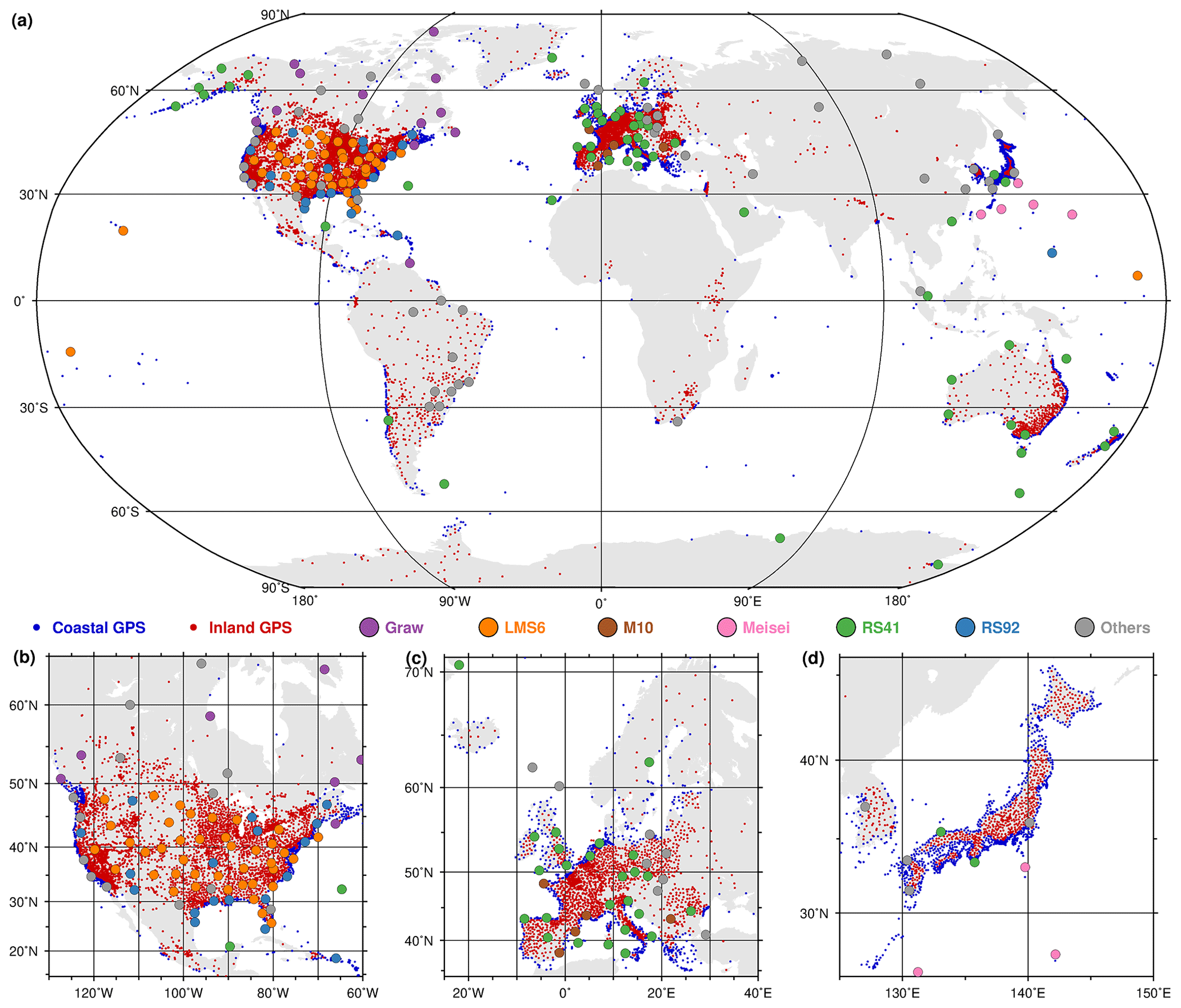
Figure 1(a) Geographical distribution of the 12 555 GPS stations and 182 radiosonde stations. (b–d) Zoomed-in figures for the USA, Europe, and Japan, respectively. There are 3745 GPS stations located within 20 km of the coastline, and they are labelled as coastal GPS (blue dots), whereas the other 8810 stations are labelled as inland GPS (red dots). The different radiosonde types are labelled in various colours.
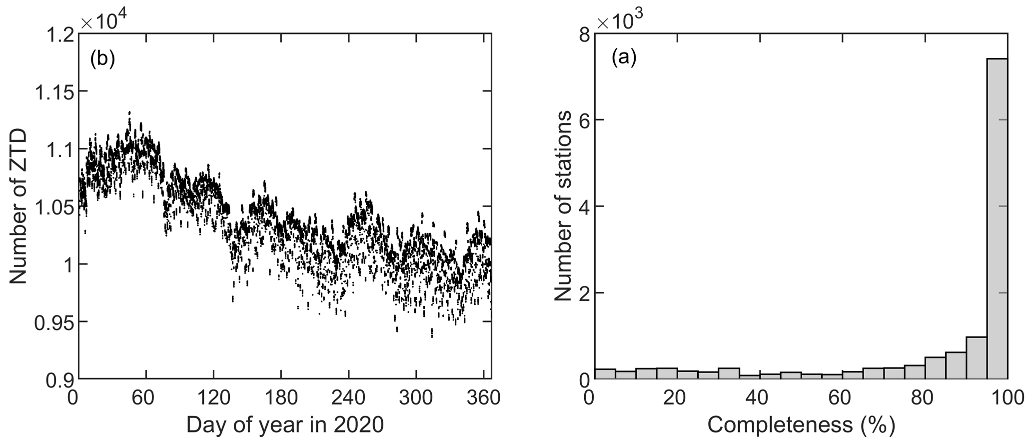
Figure 2(a) The number of raw GPS ZTD estimates of the 12 555 stations at each 5 min epoch. (b) Statistics of completeness rates of the stations. The completeness rate of a given GPS station was calculated as the ratio between the number of its ZTD estimates and the full number of 5 min epochs in 2020 (i.e. 105 408).
2.2 Screening of zenith total delay (ZTD)
Although quality control has been implemented in the GPS data pre-processing and processing, a small number of low-quality and erroneous estimates is unavoidable. Therefore, we screened the GPS ZTD estimates and their formal errors (σZTD) by employing a general range check and a station-specific outlier check (Bock et al., 2020). The range check is intended to exclude apparently unrealistic outliers. To determine a reasonable ZTD range, we calculated the global ZTD by using the 1-hourly ERA5 product and found that the ZTD at the Earth's surface was between 1096.5 and 2835.8 mm in 2020 (see Appendix A). We therefore set the ZTD range from 1000 to 3000 mm, which is believed to be wide enough to preserve all the natural variations over the world. In addition, the formal errors of the ZTD (σZTD) are a good indicator of its quality. We rejected σZTD estimates larger than 6 mm. This threshold is appropriate for GPS ZTD solutions produced using GIPSY as reported by Bock et al. (2020). Three stations were discarded, as their σZTD values were completely out of range. On average, the range checks of the ZTD and σZTD rejected 0.1 % of the data points.
The ZTD and σZTD outlier checks were conducted with station-specific thresholds. For the σZTD, an upper limit of 2×median(σZTD) was used as recommended by Bock et al. (2020), where median(σZTD) is the median value of a given station's σZTD within the whole year. Unlike σZTD, the temporal variations of the ZTD can be very complicated. We therefore used a moving window outlier detection approach with the interquartile range (IQR) rule (Upton and Cook, 1996). For the 5 min ZTD series in each day, we determined the threshold as [, ], where . The Q1 and Q3 are the 25th and 75th percentiles of all the 5 min ZTD data in a 15 d window centred on this day, respectively. This approach is more robust compared to the traditional approach based on standard deviations of the ZTD residuals from a curve fitting. As an example, Fig. 3 illustrates the data screening method at station HCRL. Outliers in the σZTD and the ZTD of HCRL were successfully excluded. Overall, the outlier checks took four iterations on average for all the stations and removed 0.33 % of the data points.
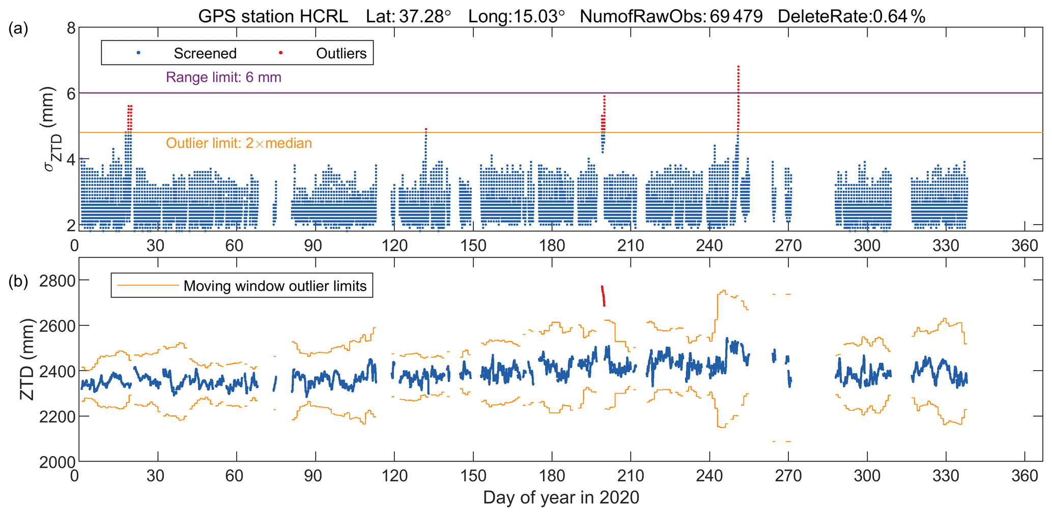
Figure 3An example of the ZTD data screening at station HCRL. (a) Range check (purple line) and station-specific robust outlier check (orange line) of σZTD. (b) Robust outlier check (orange line) of the ZTD with a 15 d moving window. The range check of the ZTD was not shown, because all the raw ZTD estimates are within the range (1000–3000 mm).
2.3 Retrieval approach of integrated water vapour (IWV)
The screened GPS ZTD estimates were then converted into IWV by using the equations of (Bevis et al., 1992)
where Π is the conversion factor (in kg m−2 mm−1), and RV=461.522 J kg−1 K−1 (Kestin et al., 1984) is the specific gas constant for water vapour. The parameters K hPa−1 and k3=373 900 K2 hPa−1 are atmospheric refractivity constants (Bevis et al., 1994). Tm denotes weighted mean temperature (in K). In the development of the enhanced GPS (enGPS) IWV product, we calculated Tm at a given GPS station based on ERA5 pressure level product (1-hourly, , and 37 vertical pressure levels) and the equation as follows:
where e and T are water vapour pressure (in hPa) and temperature (in K) profiles from the geopotential altitude (i.e. geopotential height, Hgp) of the GPS station (Hs) to the top pressure level of ERA5 (Htop). Note that all the altitudes in this paper refer to Hgp with a unit of geopotential metre (gpm) unless expressly specified. The Hgp is the altitude of a station above mean sea level (MSL) by considering the variation of gravity. It is different from ellipsoidal and orthometric heights which are commonly used in GPS and geodesy. The conversions of the height systems are provided in Appendix B. Moreover, in order to obtain the Tm at the location of the GPS station, vertical adjustment (interpolation or extrapolation) and horizontal interpolation of associated meteorological variables from the gridded ERA5 product were carried out (see Appendix C).
The ZHD used in the enGPS IWV was calculated as follows (Saastamoinen, 1972; Davis et al., 1985):
where Ps is GPS station pressure (in hPa) which is also estimated by vertical adjustment and horizontal interpolation of the ERA5 pressure level product (see Appendix C). φs and Hs are latitude (in rad) and orthometric height (in m) of the GPS station. The ERA5-derived 1-hourly ZHD and Tm were then linearly interpolated into 5 min time series and used for the retrieval of the enGPS IWV product together with NGL's ZTD.
Equations (1)–(4) indicate that Tm and the ZHD (or Ps) are essential for the calculation of GPS IWV. The relative error of IWV due to an error of ΔTm in Tm can be estimated as follows:
where K−1 is close to zero, and hence the relative error of IWV and Tm are approximately identical (Wang et al., 2005). Accordingly, 1 K of Tm error can result in a relative error of 0.33 %–0.48 % in IWV, given that the ERA5-derived global surface Tm ranges between 208.9 and 304.9 K in 2020 (see Appendix A). The ZHD error is proportional to the associated IWV error with the factor of −Π, which can be calculated from Tm. For the range of global Tm in 2020, the value of Π ranges between 0.12 and 0.17 kg m−2 mm−1.
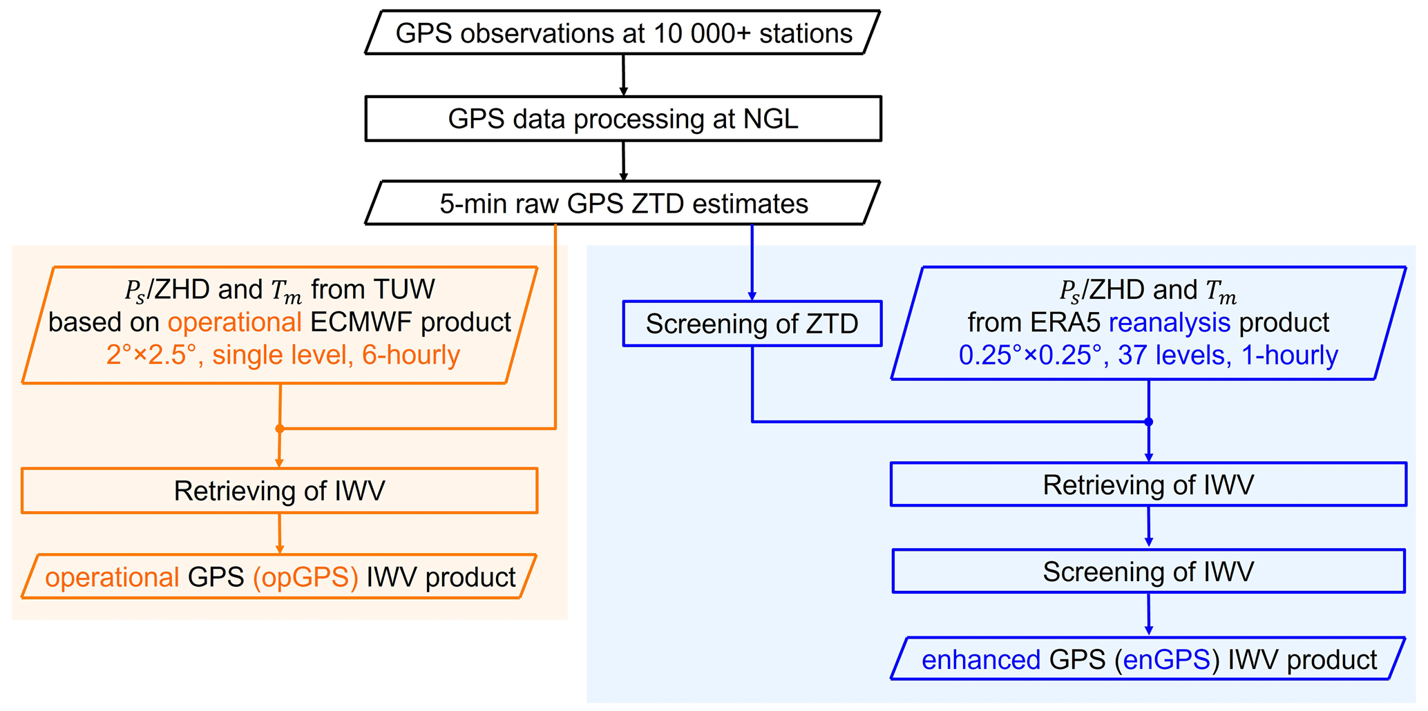
Figure 4Comparison of NGL's operational GPS (opGPS) IWV product and the enhanced GPS (enGPS) IWV product developed in this work.
2.4 Screening of IWV
The 5 min enGPS IWV data were screened with a range check and a moving window outlier check. We first determined the IWV range by inspecting global IWV at the Earth's surface derived by ERA5 (see Appendix A). Results showed that the global IWV in 2020 ranges from 0.0 to 94.9 kg m−2 (Fig. A1a and b). We therefore set the range of the check as 0–100 kg m−2. The range check showed that no data point in the enGPS IWV product has a value larger than 100 kg m−2. However, 0.03 % (292 143) data points showed values less than zero, which could be due to inaccurate ZTD or ZHD estimates. The physically unrealistic estimates were mostly found at high-latitude stations with complex terrains, such as Antarctica and Greenland. These sites have low humidities and might have large spatial interpolation errors in the ZHD. Moreover, the moving window outlier check rejected 0.16 % of the IWV data points.
In the end, we obtained 1 093 591 492 5 min enGPS IWV estimates at 12 552 stations in 2020, which is equal to 87 125 data points per station and 10 375 data points every 5 min. The average completeness rate was 82.7 %, and the rates were higher than 95 % at 7253 stations.
2.5 Enhancements compared to NGL's operational IWV product
Figure 4 compares the development processes of NGL's operational GPS (opGPS) IWV product and the enhanced GPS (enGPS) IWV product developed in this work. The enhancements are mainly in the auxiliary meteorological data for GPS IWV retrieval and the data screening.
The ZHD and Tm used in NGL's operational IWV product were obtained from the Vienna University of Technology (TUW, https://vmf.geo.tuwien.ac.at/, last access: 27 January 2023) during the GPS data processing. TUW calculates the ZHD and Tm every 6 h at the Earth's surface with a grid based on an operational ECMWF product (Boehm et al., 2006). Although vertical adjustments of both ZHD and Tm from the ECMWF surface level to the altitude of the GPS station are essential for the accurate calculation of GPS IWV, only the ZHD was vertically adjusted in NGL's opGPS IWV product with an empirical formular as described in Appendix D. The vertical change of Tm has not been considered in the opGPS IWV product, because an accurate lapse rate of Tm is hard to obtain from the surface level product. In comparison, the enGPS IWV product was developed by using the meteorological data from the state-of-the-art ERA5 reanalysis with 1-hourly estimates at horizontal grids and 37 vertical pressure levels, with more advanced vertical adjustment correction algorithms as described in Sect. 2.3 and Appendix C. Moreover, despite non-real time, the atmospheric reanalysis products are generally considered to be superior to the operational analysis products due to improvements in input data and assimilation algorithms (Dee, 2009). Therefore, the meteorological data obtained from ERA5 are expected to be more accurate than those from TUW.
As for the quality control of the product, we carried out dedicated data screening (range check and outlier check) on the GPS ZTD and enGPS IWV time series as described in Sect. 2.2 and 2.4, respectively. However, these data screening steps were not included in the opGPS IWV product provided by NGL.
For a fair comparison to the enGPS IWV product in this work, we also screened the opGPS IWV product with the same algorithm in Sect. 2.4. The range check excludes 0.35 % (3 849 630) of the data points with unrealistic negative IWV estimates, which is 13 times larger than that of enGPS. In particular, the IWV at four stations (CON2, MCG2, NAU2, and PHIG) on the high mountains (>3000 gpm) of Ross Island, Antarctica, were entirely smaller than zero in opGPS but rarely negative in enGPS. As an example, Fig. 5 compares their IWV estimates at station PHIG (77.53∘ S, 167.05∘ E; 3185.9 gpm). All the opGPS IWV estimates are unrealistically below zero, with values ranging from −13.0 to −1.7 kg m−2. In contrast, the enGPS IWV estimates are between −0.3 and 2.5 kg m−2 with negative values at only 0.32 % (335 out of 105 389) of the data points. The negative opGPS IWV estimates at station PHIG are likely caused by the inaccurate ZHD provided by TUW with low spatial resolution and an unrealistic approximation of the barometric formula (Eq. D1) used to adjust pressure from the TUW model surface to an extremely high altitude. The results indicate that the enGPS IWV product is much superior to the opGPS IWV product in avoiding unrealistic negative IWV estimates, especially at the stations with high altitudes. Therefore, the enGPS IWV product is recommended for those regions.
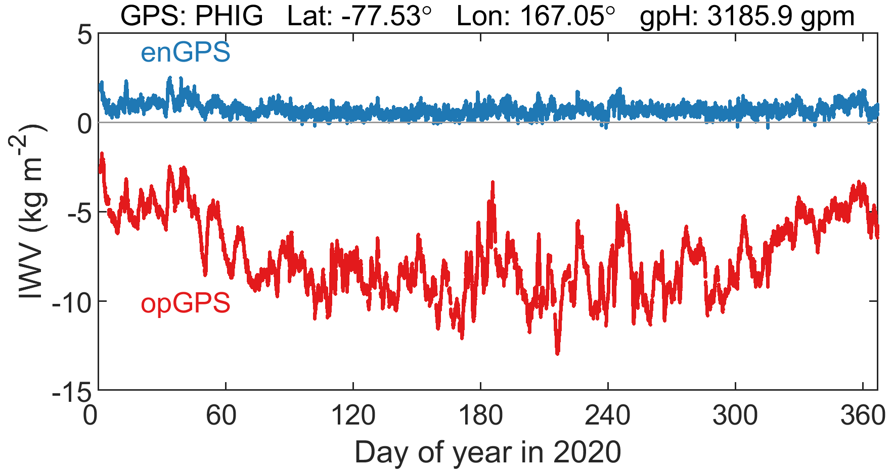
Figure 5Comparison of the unscreened enGPS (blue) and opGPS (red) IWV at station PHIG (77.53∘ S, 167.05∘ E; 3185.9 gpm). Hgp is geopotential altitude in geopotential metre (gpm; see Appendix B).
2.6 In situ meteorological observations
Intercomparison of IWV products derived by different techniques is crucial for the evaluations of their consistency and quality. In this work, we aggregated the 5 min GPS IWV and associated Tm and ZHD data into 1-hourly time series with a threshold of at least four 5 min data points in each moving 1 h time window centred at a full hour. We then compared the 1-hourly enGPS and opGPS IWV products and their Tm values with those of in situ radiosonde (RS) observations collected by the Integrated Global Radiosonde Archive (IGRA) version 2 (Durre et al., 2018). RS measurements have traditionally been used as validation sources for other humidity measurements (e.g. Lindstrot et al., 2014). IGRA is one of the most comprehensive RS datasets consisting of over 2800 stations worldwide, of which 770 were operational with regular daily observations at 00:00 and 12:00 UTC in the year of 2020. We used temperature and relative humidity profiles from the IGRA dataset and carried out quality control with the following criteria: (1) the profiles reach the surface and a pressure level of at least 300 hPa on top (Wang and Zhang, 2008), (2) data are available at no less than five (four) standard pressure levels for stations below (above) the 1000 hPa pressure level (Wang et al., 2005), and (3) pressure gaps should be less than 200 hPa.
In addition to Tm, the quality of the ZHD also has an influence on GPS IWV retrievals. We employed the ZHD calculated by using synoptic (SYN) observations from the Integrated Surface Database (ISD; Smith et al., 2011) as references to evaluate the ZHD values estimated from ERA5 and TUW. ISD has more than 20 000 SYN stations worldwide and provides high-quality observations (e.g. pressure) with internal quality control procedures. In the year of 2020, the pressure observations were available at 11 637 ISD stations worldwide.
We analysed the statistical characteristics of each 5 min enGPS IWV time series by calculating the minimum, maximum, and mean value, as well as the coefficient of variation (CV), which is the ratio of the SD to the mean. To avoid impacts of missing data on the estimates, we selected 9418 out of the 12 552 stations with a criterion that their completeness rates were higher than 50 %, and their data gaps were shorter than 30 d. The IWV time series of the selected stations range from 0 to 82.7 kg m−2 (Fig. 6a and b). The geographical patterns of the minima and maxima of the GPS IWV are consistent with those from ERA5 (Fig. A1a and b). The minima of the GPS IWV generally increase towards the Equator with values close to zero at the poles (66.5–90∘ N or 66.5–90∘ S) and median values of 1.5 and 9.1 kg m−2 in mid-latitude (23.5–66.5∘ N or 23.5–66.5∘ S) and tropical (23.5∘ N–23.5∘ S) zones, respectively. However, the geographical characteristics of the maxima IWV are more complicated, as they depend on climate type and altitude in addition to latitude. The lower maxima were observed at the polar climate zones or high-altitude regions with the lowest value of 2.2 kg m−2 at station NAU2 (77.52∘ S, 167.15∘ E; 3632 gpm) on Ross Island, Antarctica (Fig. 6e). Moreover, the maxima of most of the stations in Antarctica are generally lower than 10 kg m−2 except for the Antarctic Peninsula. This is not surprising, because Antarctica is known as the coldest, driest, and highest continent on Earth. In contrast, the monsoon zones or low-altitude regions are characterised with larger maxima by the largest value of 82.7 kg m−2 at station J731 (28.37∘ N, 130.03∘ E; 11 gpm) on the Ryukyu Islands, Japan, during Typhoon Haishen on 6 September 2020.
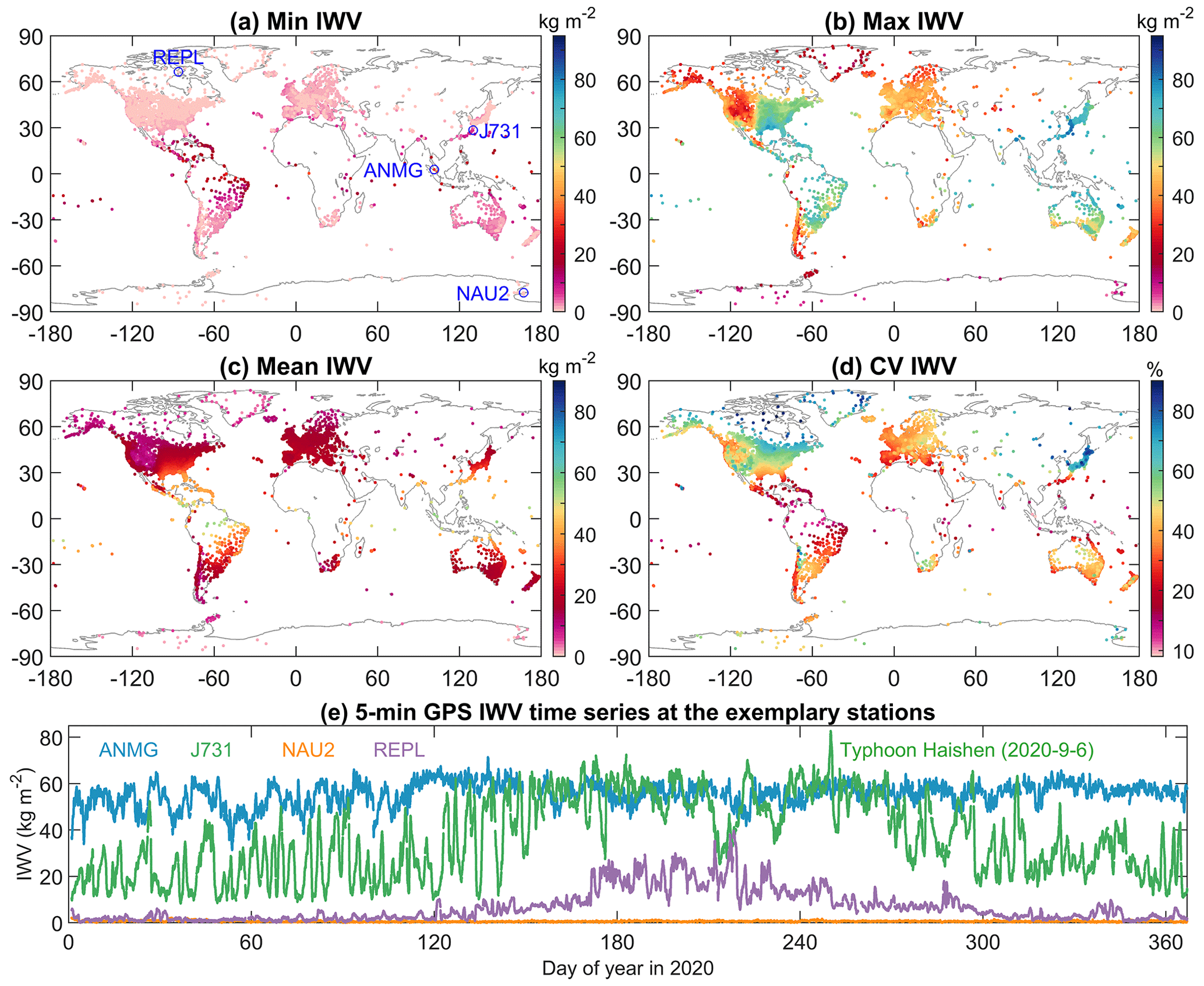
Figure 6Minima (a), maxima (b), mean values (c), and coefficients of variations (d) of the 5 min enhanced GPS IWV time series in 2020 at 9418 stations. (e) IWV time series of four exemplary stations.
The mean values of the stations' IWV estimates generally increase towards the Equator, with the lowest and highest values of 0.6 and 55.5 kg m−2 found at station NAU2 in Antarctica and ANMG (2.8∘ N, 101.51∘ E; 18 gpm) in Malaysia, respectively. As can be seen in Fig. 6e, the variation of IWV at station ANMG is rather small compared to its mean value, and hence, it has one of the lowest CVs with a value of 9.1 % (Fig. 6d). In contrast, the largest CV with a value of 100 % is observed at station REPL (66.52∘ N, 86.23∘ W; 21 gpm) at Repulse Bay, Canada, where both the mean and SD of IWV are equal to 6.9 kg m−2 (Fig. 6e).
As described in Sect. 2.6, there were 770 RS and 11 637 ISD stations available in 2020. In order to evaluate the opGPS and enGPS IWV products, we carried out a spatial and temporal matching of the GPS, RS, and ISD stations with the following criteria: (1) the distances of the RS and SYN stations with respect to their paired GPS stations are within 50 km in horizontal and 100 m in vertical (Wang and Zhang, 2008), and (2) the time-matched GPS, RS, and SYN observations are available at more than 50 % of the 00:00 and 12:00 UTC epochs in 2020, and all the gaps in time are shorter than 30 d. The second criterion on data availability is necessary, because the IWV differences from opGPS or enGPS with respect to RS can be seasonal dependent as discussed later in Sect. 5 (Fig. 13). The seasonal patterns can also be seen in the differences in Tm and ZHD. Therefore, the second criterion was applied to avoid incorrect explanations. It is noteworthy that 328 out of the 770 radiosonde stations had been discarded before the matching, because their observations are only available at less than 50% of the 00:00 and 12:00 UTC epochs in 2020, or their gaps in time are longer than 30 d. With those criteria, we obtained 182 GPS–RS–SYN station clusters worldwide. The locations of the station clusters are listed in Table S1 in the Supplement.
We conducted vertical adjustments of humidity, temperature, and pressure observed at the RS to the altitude of their paired GPS station and then calculated the associated IWV and Tm. We also adjusted the SYN pressure measurements vertically to the altitude of their paired GPS station for the calculation of referenced ZHD. Details of the vertical adjustments of RS and SYN observations are provided in Appendix C. After that, we screened the IWV differences by employing a 3-fold IQR rule with a 90 d moving window. Similarly, the Tm differences and ZHD differences were also screened.
Figure 7a shows the mean RS–enGPS IWV differences at the 182 station clusters. The values are within ±3 kg m−2. North America is characterised by a general negative mean IWV difference, indicating a dry bias of RS with respect to enGPS or a wet bias of enGPS with respect to RS. In contrast, the differences are positive at a part of European stations, indicating a wet bias of RS or a dry bias of enGPS. The IWV biases could be due to systematic errors and technique-related differences in RS and GPS, as well as inaccurate meteorological information. We expand a little further on this.
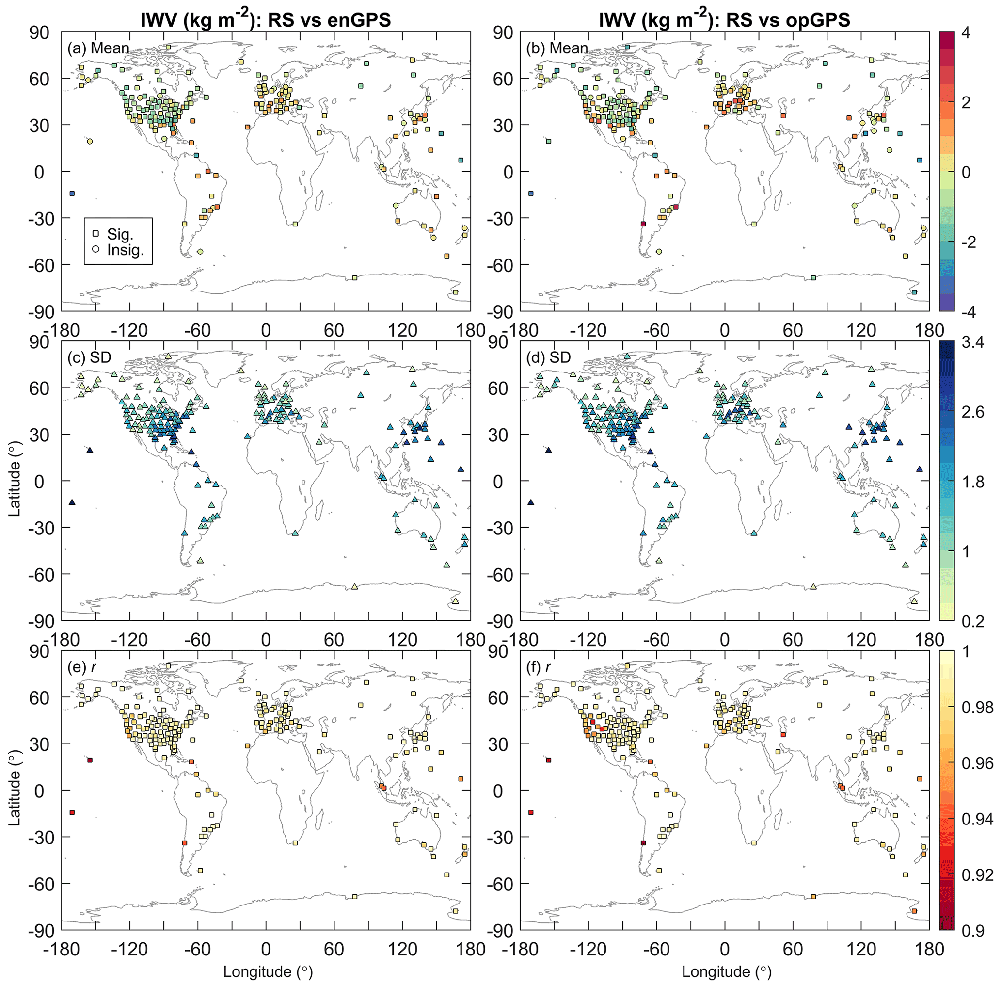
Figure 7Comparisons of IWV from radiosonde observations and those from enGPS (a, c, e) or opGPS (b, d, f) IWV retrievals at 182 station clusters in mean value (a, b) and standard deviation (c, d) of their differences (radiosonde minus GPS) and Pearson correlation coefficient (e, f). The enGPS and opGPS indicate the enhanced GPS IWV product developed in this work and the operational GPS IWV product provided by NGL, respectively. The significant (squares) and insignificant (circles) mean values and correlation coefficients are derived from tests at 95 % confidence level.
As humidity biases in specific RS types are well known (e.g. Wang and Zhang, 2008), they are investigated first. We classified the RS stations into seven subsets (namely Graw, LMS6, M10, Meisei, RS41, RS92, and “others”) according to their manufacturers and sensor types in 2020 (Fig. 1). The subset of others includes stations with unknown types or type changes. Figure 8 shows the IWV difference between RS and enGPS for each subset. Good agreements are observed in the subsets of Meisei, RS41, and RS92 with mean IWV differences of −0.4, 0.3, and 0.5 kg m−2, respectively. However, the Graw and LMS6 stations, mostly located in North America and the Pacific, are generally characterised by noticeable negative mean RS–enGPS IWV differences down to −3.0 with averages of −0.9 and −1.1 kg m−2, respectively. In contrast, the M10 stations, all located in Europe, obtain positive mean RS–enGPS IWV differences ranging from 0.5 to 1.3 with an average of 1.0 kg m−2.

Figure 8Mean values and standard deviations of the IWV differences (radiosonde minus enGPS) at the 182 station clusters. The colours of the bars indicate different radiosonde types.
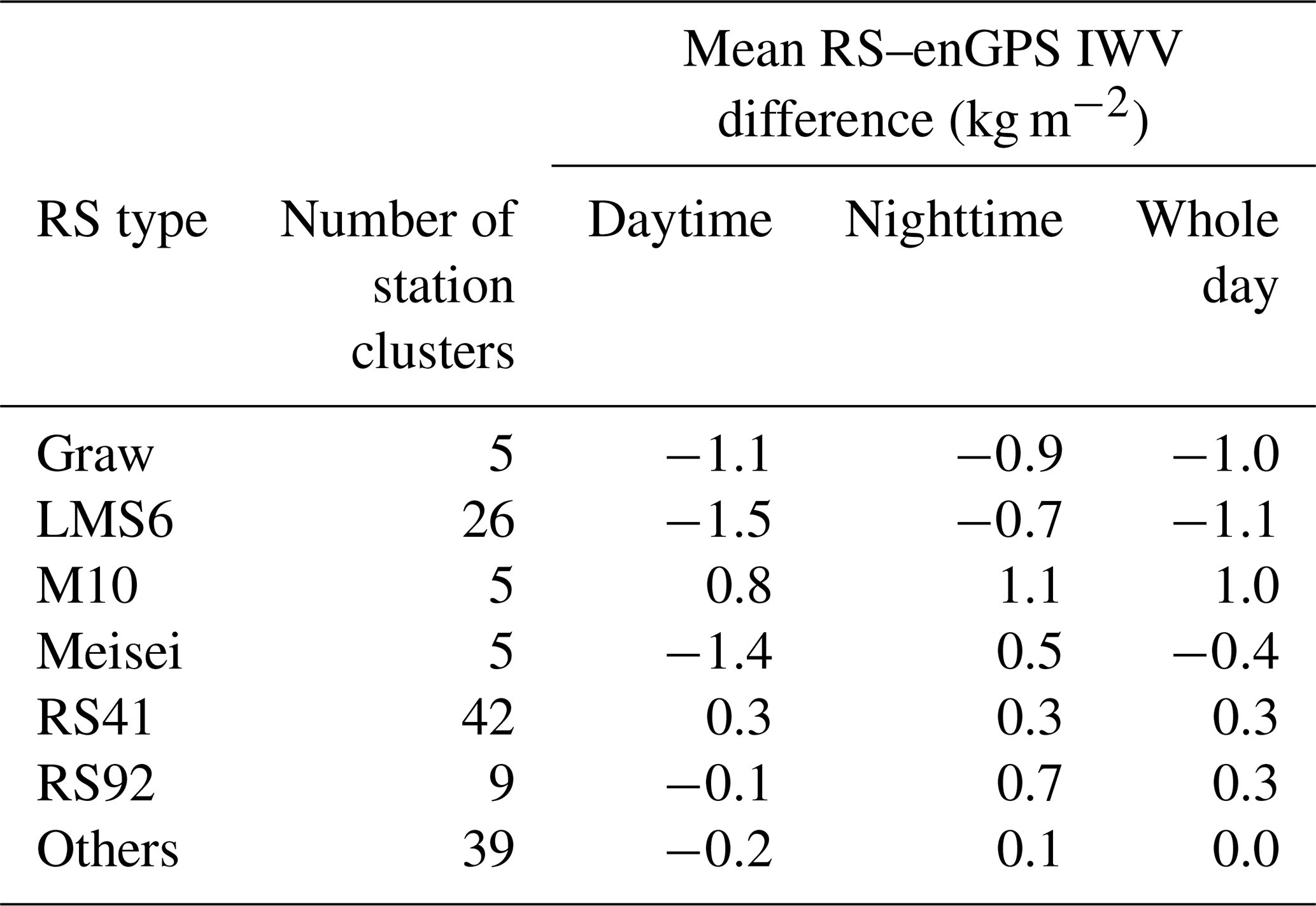
As the RS humidity measurements could be impacted by solar radiation bias, we further evaluated and compared the IWV biases of RS with respect to GPS at daytime and nighttime. The daytime and nighttime of a RS station were determined as its time of 08:00–18:00 and 20:00–06:00 LT (local time), respectively. Stations with their observations available at the time of 06:00–08:00 LT (dawn) or 18:00–20:00 LT (twilight) were excluded. Stations in polar regions (66.5–90∘ S or 66.5–90∘ N) were also removed. In the end, there are 131 out of the 182 RS–enGPS station clusters selected for the daytime and nighttime comparison. Table 1 lists the mean RS–enGPS IWV difference at daytime, nighttime, and in the whole day for each RS type. Both mean RS41–enGPS IWV differences at daytime and nighttime are identical to a small value of 0.3 kg m−2, indicating a good agreement between RS41 and GPS in both scenarios. However, although the mean Meisei–enGPS IWV difference is small in the whole day (−0.4 kg m−2), it is an average of the significant negative value at daytime (−1.4 kg m−2) and the moderate positive value at nighttime (0.5 kg m−2), respectively. Likewise, the mean RS92–enGPS IWV differences are −0.1, 0.7, and 0.3 kg m−2 at daytime, at nighttime, and in the whole day, respectively. The results suggest that it is important to evaluate the mean RS–enGPS IWV difference at daytime and nighttime separately, even though the mean difference in the whole day is small. Moreover, both the mean LMS6–enGPS IWV differences at daytime and nighttime are negative with values of −1.5 and −0.7 kg m−2, respectively. The results indicate a stronger dry bias of LMS6 with respect to enGPS at daytime than nighttime. Similar results are seen in Graw. The mean Graw–enGPS IWV differences are −1.1 and −0.9 kg m−2 at daytime and nighttime, respectively. By contrast, the mean M10–enGPS IWV differences are positive at daytime and nighttime with values of 0.8 and 1.1 kg m−2, respectively. In addition, we also investigated the GPS receiver and antenna types of these station clusters, but we did not find obvious relationships with the IWV differences. The results suggest that the mean RS–enGPS IWV differences might be more related to the RS types rather than the GPS types, but other factors like inaccurate meteorological information cannot be excluded.
Table 1Mean IWV differences between RS and enGPS at daytime, nighttime, and in the whole day. The daytime and nighttime were determined as observations of stations within 66.5∘ S–66.5∘ N at 08:00–18:00 and 20:00–06:00 LT, respectively. Accordingly, stations at 90–120∘ E and 60–90∘ W were excluded, because their time is 06:00–08:00 LT (dawn) or 18:00–20:00 LT (twilight) at 00:00 and 12:00 UTC, at which the RS observations are available. In the end, 131 out of the 182 RS–enGPS station clusters were selected for the daytime and nighttime comparison.
Inaccurate meteorological information could deteriorate GPS IWV retrievals. Section 2.3 has indicated that the relative error of Tm and the associated relative error of IWV are approximately equal, while 1 mm ZHD bias can result in an IWV bias ranging from 0.12 to 0.17 kg m−2. In order to find out why the mean RS–enGPS IWV difference for the Graw, LMS6, and M10 is more significant than the other types, we compared the ERA5-derived Tm and ZHD with reference values from the in situ RS and SYN observations, respectively. The mean RS–ERA5 Tm differences are 0.2–2.3 K for the 55 Graw and LMS6 station clusters (Fig. 9a), equivalent to relative Tm differences of 0.1 %–0.8 %, whereas the associated relative RS–enGPS IWV differences are −17.2 % to 0.3 % with an average of −6.5 %. Likewise, the relative RS–ERA5 Tm differences for the five M10 station clusters are 0 %–0.2 %, whereas the associated relative RS–enGPS IWV differences are 2.6 %–6.3 % with an average of 4.7 %. Regarding the ZHD, the mean SYN–ERA5 difference is −0.7 mm for the Graw and LMS6 station clusters (Fig. 10a), which would only result in an average IWV bias of 0.1 kg m−2, but the actual value is −1.0 kg m−2. As for the M10 station clusters, their mean SYN–ERA5 ZHD difference is −0.6 mm, suggesting a mean RS–enGPS IWV difference inferior to 0.1 kg m−2, which is an order of magnitude lower than the actual value of 1.0 kg m−2. The results indicate that the errors of the ERA5-derived Tm and ZHD are very unlikely to be the primary reason for the significant RS–enGPS IWV for these three RS types. Although it seems that the systematic differences in RS–enGPS IWV are related to the specific RS types, we cannot exclude other factors, such as GPS data processing models and strategies. Intercomparisons with other water vapour retrieval techniques will contribute to a more comprehensive understanding of the disagreements, but it is beyond the scope of this work and will be addressed in the future.

Figure 9Comparisons of Tm from radiosonde observations and those from ERA5 (a, c, e) or TUW at 182 station clusters in mean value (a, b) and standard deviation (c, d) of their differences (radiosonde minus ERA5 or TUW) and Pearson correlation coefficient (e, f). The Tm obtained from ERA5 and TUW were used in the retrievals of enGPS and opGPS IWV products, respectively.

Figure 10Comparisons of the ZHD from synoptic (SYN) pressure observations and those from ERA5 (a, c, e) or TUW at 182 station clusters in mean value (a, b) and standard deviation (c, d) of their differences (SYN minus ERA5 or TUW) and Pearson correlation coefficient (e, f). The ZHD obtained from ERA5 and TUW were used in the retrievals of enGPS and opGPS IWV products, respectively.
The enGPS IWV product is different from opGPS in the fact that the conversion of IWV from the ZTD was carried out by using the high spatiotemporal resolution reanalysis ERA5 instead of TUW, and thus a quality improvement is expected. We assess the quality of both GPS IWV datasets by taking the IWV from RS as reference. We are aware that the IWV measured by specific RS types could be biased, and thus we will interpret the results with caution by considering differences in the meteorological data for GPS IWV retrieval and the topographical complexity of terrains around the stations.
Figure 11 compares the IWV consistency in mean value and SD of RS–GPS differences, as well as linear Pearson correlation coefficient, at each station cluster. The majority of the mean RS–GPS IWV differences are within ±3 kg m−2 for both enGPS and opGPS (Fig. 11a). However, the mean absolute bias (MAB) decreases from 0.86 to 0.69 kg m−2 by the development of enGPS, equal to a reduction of 19.5 %. In particular, the mean IWV differences in RS–opGPS turn out to be negligible in RS–enGPS at several stations, e.g. stations NAVI, PAVI, and J500 with values from 8.0, 2.5, and −2.8 to 0.3, 0.3, and 0.2 kg m−2, respectively. Their improvements will be carefully analysed in the latter part of this section. In addition, enGPS IWV has a better agreement with RS in variability. Compared to opGPS, the average SD of IWV differences decreases from 1.58 to 1.48 kg m−2, indicating a reduction of 6.2 % (Fig. 11b). The most significant SD reduction can be found at station PAVI, with its SD decreasing from 2.5 to 1.4 kg m−2. Also, enGPS IWV achieves a slightly stronger correlation with respect to RS than that between opGPS and RS, with average correlation coefficients of 0.986 and 0.983, respectively. The correlation improvement is more significant at specific stations (Fig. 11c). For example, the correlation coefficient is increased from 0.89 to 0.94 at station NAVI. Inspecting the maps of IWV comparisons shown in Fig. 7, we find that the improvements in the IWV agreements are most significant in regions with a considerable topographical complexity of terrains, such as the Alps, Rocky Mountains, Andes, and Antarctic coast. The results indicate that enGPS IWV is superior to opGPS.
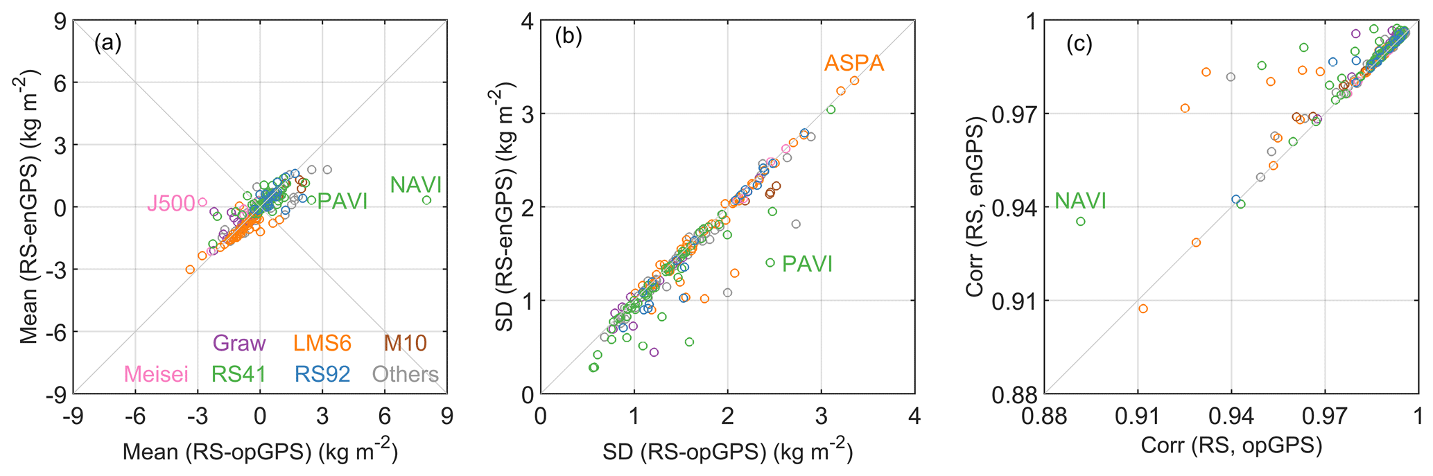
Figure 11Comparisons of the mean values (a) and standard deviations (b) of the IWV differences between radiosonde and opGPS or enGPS and correlations (c) between IWV from radiosonde and opGPS or enGPS. The colours of the circles indicate different radiosonde types.

Figure 12(a) Mean absolute altitude difference (between the altitudes of each GPS station and its four surrounding TUW grid nodes indicated by the sizes of circles. The colours of the circles indicate the radiosonde types as shown in Fig. 1. The grey-scale grids are the geopotential altitudes of the TUW model surface converted from ellipsoid heights (see Appendix B). (b) Altitudes of the nine GPS stations with their larger than 1000 gpm. The orange and blue bars indicate the altitudes of GPS stations and their specific four surrounding TUW grid nodes, respectively.
To explain the improvements in IWV agreements, we evaluated the meteorological information from ERA5 and TUW by taking the RS-derived Tm and SYN-derived ZHD as references, respectively. Figures 9 and 10 show that the ERA5-derived Tm and ZHD outperform those from TUW with the most striking improvements also in regions with complex topographical terrains. The results indicate that the enhancements of ERA5 in spatial resolution (, 37 levels) might enable us to resolve local variations of the meteorological variables in the complex topographical areas. To evaluate the impacts of complex terrains on the performance of the TUW product, we calculated the mean absolute altitude difference () for each GPS station:
where Hs and Hi (i=1, 2, 3, 4) are the altitudes of the GPS station and its four adjacent TUW grid nodes, respectively. The is considered a topographical complexity index as displayed in Fig. 12a. When the is larger, the spatial representativeness differences between the in situ meteorological observations and the gridded TUW products tend to be more significant. It is seen from Fig. 12a that the values are larger in the Alps and Rocky Mountains. In addition, extreme values of can also be observed at the Andes and Antarctic coast, despite the fact that there are only a few stations there. Figure 12b illustrates the altitudes of nine stations whose are larger than 1000 gpm. The largest value of is found at station NAVI with a value of 2160 gpm.
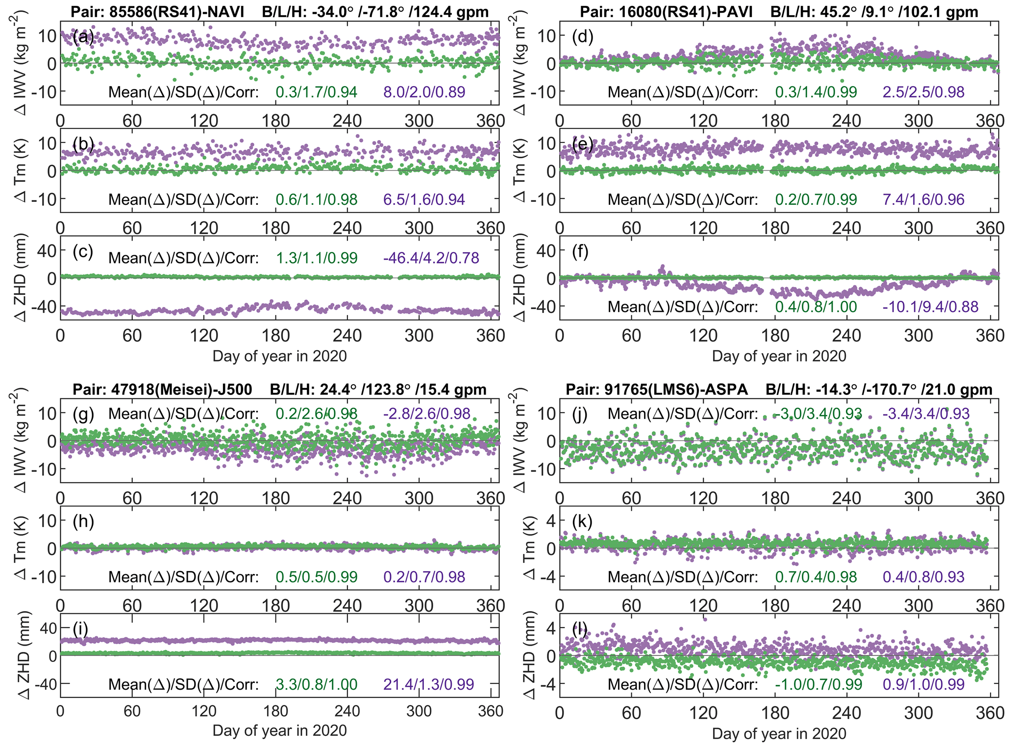
Figure 13(a) IWV differences between radiosonde (RS) observations and enGPS (green) or opGPS (purple) at station cluster 85586-NAVI. (b) Tm differences between radiosonde and ERA5 for enGPS (green) or TUW for opGPS (purple). (c) ZHD differences between synoptic (SYN) observations and ERA5 (green) or TUW (purple). Panels (d, g, j), (e, h, k), and (f, i, l) are the same as (a), (b), and (c) but for the other three station clusters, respectively. Note that the ranges of y axes in (k) and (l) are different from the others.
Station NAVI (34.0∘ S, 71.8∘ W; 124.4 gpm) is located at a coastal area of Chile between the Pacific and the rugged Andes. Two of its four adjacent grid nodes are close to mean sea level, while the other two are higher than 4200 gpm. We analysed the impacts of spatial representativeness difference due to the strong variations of topographical relief on the estimates of its IWV, as well as associated Tm and ZHD (Fig. 13a–c). The mean IWV difference reaches 8.0 kg m−2 at NAVI for RS–opGPS but reduced to 0.3 kg m−2 for RS–enGPS. The results indicate relative mean IWV differences of 58 % and 2 %, respectively, by referring to its RS-derived IWV with a mean value of 13.8 kg m−2. As for the associated Tm, the mean differences in RS–ERA5 and RS–TUW are 0.6 and 6.5 K (i.e. 0.2 % and 2.3 %), respectively. Moreover, the mean ZHD differences in SYN–ERA5 and SYN–TUW are 1.3 and −46.4 mm, respectively. As we know that the relative bias of Tm results in nearly the same amount of relative bias of IWV, the IWV biases due to Tm should be only 0.0 and 0.3 kg m−2 for RS–enGPS and RS–opGPS, respectively. In contrast, the IWV biases due to the ZHD are −0.2 and 7.4 kg m−2 in RS–enGPS and RS–opGPS, respectively, by assuming Π=0.17 in Eq. (1). Therefore, the considerable mean SYN–TUW ZHD difference at station NAVI is likely to be the primary reason for its large mean RS–opGPS IWV difference. Similar results are also observed at many other stations situated in regions with complex topography, such as the Alps, Rocky Mountains, and Antarctic coast (see e.g. Figs. 7–9). The results indicate that the improvement of ERA5 in spatial representativeness with respect to TUW enables a significant mitigation of mean IWV difference in RS–enGPS with respect to RS–opGPS.
The RS–opGPS IWV difference can also be dependent on season. For example, it can be as large as 10.5 kg m−2 in summer whereas mostly within ±2 kg m−2 in winter at station PAVI (45.2∘ N, 9.1∘ E; 102.1 gpm; Fig. 13d), which is in northern Italy at the foothills of the Alps. Similarly, its SYN–TUW ZHD difference time series is also characterised with a strong seasonal pattern with a SD of 9.4 mm (Fig. 13f). As the of station PAVI is quite large (1418 gpm), its seasonal-dependent RS–opGPS IWV difference can be attributed to the strong spatial representativeness difference of the gridded TUW-derived ZHD with respect to that from the in situ SYN. By contrast, the seasonal variation of the SYN–ERA5 ZHD difference is quite weak, with an SD of only 0.8 mm. As a result, the SD of the IWV difference is reduced from 2.5 in RS–TUW to 1.4 kg m−2 in RS–ERA5 for this station. The results indicate that ERA5 has a better spatial representativeness of seasonal variations of ZHD than TUW at station PAVI and thus contributes to more accurate GPS IWV retrievals over time.
In addition, the benefit of the enhanced spatial representativeness of ERA5 with respect to TUW is also significant for stations on islands and in coastal regions. For instance, the mean ZHD difference is reduced from 21.4 mm in SYN–TUW to 3.3 mm in SYN–ERA5 at station J500 (24.4∘ N, 123.8∘ E; 15.4 gpm) on an island of Okinawa, Japan (Fig. 13i). Consequently, the mean IWV difference has been substantially reduced from −2.8 kg m−2 in RS–opGPS to 0.2 kg m−2 in RS–enGPS (Fig. 13g). The more significant mean IWV difference in RS–opGPS could be due to the noticeable SYN–TUW ZHD differences with an average of 21.4 mm (Fig. 13i), which could result in an IWV bias in the range from −3.6 to −2.6 kg m−2.
There are also stations at which the IWV differences cannot be properly explained by the spatial representativeness differences of Tm and ZHD. For example, at station ASPA (24.4∘ S, 123.8∘ W; 15.4 gpm) on an island of Samoa, the mean IWV differences in RS–enGPS and RS–opGPS reach −3.0 and −3.4 kg m−2, respectively. Since the average IWV from RS is 47.9 kg m−2 at this station, the mean Tm differences in RS–ERA5 and RS–TUW, with values of 0.7 and 0.4 K (i.e. 0.2 % and 0.1 %), would only lead to mean IWV differences inferior to 0.1 kg m−2 in both RS–enGPS and RS–opGPS. As for the mean ZHD differences in SYN–ERA5 and SYN–TUW with values of −1.0 and 0.9 mm, the corresponding absolute mean IWV differences in RS–enGPS and RS–opGPS should be less than 0.2 kg m−2. Hence, the spatial representativeness differences in Tm and ZHD are very unlikely to result in such significant IWV differences. Moreover, the distance between the station cluster of 91765-ASPA is only 1.1 km in horizontal and 17 gpm in vertical, indicating a weak representativeness difference between the GPS- and RS-derived IWV. A more likely reason could be the systematic dry bias of the LMS6 sensor as analysed in Sect. 4. Furthermore, the SD values of the RS–enGPS and RS–opGPS IWV differences are identical at station ASPA, with a value of 3.4 kg m−2 (Fig. 13j). This is the maxima SD value over all the 182 station clusters in both enGPS and opGPS IWV datasets (Fig. 11b), indicating that the poor agreement could also be due to station-specific errors in the GPS ZTD and RS IWV measurements. Further comparisons with other GPS ZTD solutions and independent IWV measurements derived by other techniques will be helpful to explain the poor agreement, and it will be addressed in future studies.
The GPS ZTD data were provided by NGL (http://geodesy.unr.edu; NGL, 2023). The auxiliary meteorological data for the retrieval of enGPS and opGPS IWV were derived by ERA5 from the Climate Data Store (CDS, https://cds.climate.copernicus.eu; ECMWF, 2023) and the GRID map product of Vienna University of Technology (TUW, https://vmf.geo.tuwien.ac.at/; TUW, 2023), respectively. The radiosonde data and synoptic data were provided by the National Centers for Environmental Information (NCEI) in the datasets of IGRA (https://www.ncei.noaa.gov/access/metadata/landing-page/bin/iso?id=gov.noaa.ncdc:C00975; NCEI, 2023a) and ISD (https://www.ncei.noaa.gov/products/land-based-station/integrated-surface-database; NCEI, 2023b), respectively. The enhanced GPS IWV dataset described in this paper is available at https://doi.org/10.5281/zenodo.6973528 (Yuan et al., 2022).
A global dataset of high-quality ground-based GPS integrated water vapour (IWV) has been developed in this work. It consists of 1 093 591 492 IWV estimates at 12 552 GPS stations worldwide in 2020 with a temporal resolution of 5 min, which is equal to 87 125 data points per station or 10 375 data points every 5 min. The dataset is derived by using precise GPS tropospheric zenith total delays (ZTD) provided by the Nevada Geodetic Laboratory (NGL), as well as zenith hydrostatic delays (ZHD) and weighted mean temperatures (Tm), obtained from the newly released ERA5 atmospheric reanalysis with a very high spatiotemporal resolution (, 37 vertical levels, 1-hourly). A dedicated robust data screening approach is also implemented in order to avoid the impacts of outliers. The dataset can be considered an enhanced version of NGL's IWV product compared to its operational version, which is produced routinely by using the meteorological information from TU Wien (TUW) with a much coarser resolution (, surface level, 6-hourly).
The global GPS IWV values ranged between 0.0 and 82.7 kg m−2 in 2020. Its stochastic characteristics can be related to many factors, such as latitude, altitude, topography, and climate type. For instance, the maxima of IWV are mostly lower than 10 kg m−2 in Antarctica with high altitude, as well as cold and dry climate condition. The average IWV of the stations generally increase from the poles towards the Equator with values from 0.6 to 55.5 kg m−2.
The enhanced GPS (enGPS) IWV product has a good agreement with global radiosonde observations. The mean absolute bias (MAB) at 182 collocated station clusters is only 0.69 kg m−2. However, systematic effects related to specific radiosonde types are noticed. Although the mean RS–enGPS IWV differences are within ±0.5 kg m−2 for types of Meisei, RS41, and RS92, they are more significant for Graw, LMS6, and M10, with values of −1.0, −1.1, and 1.0 kg m−2, respectively. In addition, the mean RS–enGPS differences at daytime and nighttime can be significantly different in specific RS types, although they are identical to 0.3 kg m−2 in RS41–enGPS IWV. For example, the mean Meisei–enGPS IWV difference at daytime and nighttime is −1.4 and 0.5 kg m−2, respectively. The values for RS92–enGPS IWV difference are −0.1 and 0.7 kg m−2, respectively. Both the mean LMS6–enGPS IWV differences at daytime and nighttime are negative with values of −1.5 and −0.7 kg m−2, respectively. Similarly, the values for Graw–enGPS IWV difference are −1.1 and −0.9 kg m−2, respectively. By contrast, both the mean M10–enGPS IWV differences at daytime and nighttime are positive with values of 0.8 and 1.1 kg m−2, respectively. The significant IWV differences in these three radiosonde types are more likely to be related to their own systematic effects (e.g. solar radiation effect) rather than GPS device types or meteorological data, but other factors cannot be excluded.
The enGPS IWV is generally superior to NGL's operational GPS (opGPS) IWV product. With the development of enGPS IWV, the mean absolute biases and standard deviations of differences with respect to radiosonde-derived IWV are reduced by 19.5 % and 6.2 % on average, respectively. The improvements are more obvious in regions with complex topographical terrains like the Alps, Rocky Mountains, Andes, and Antarctic coast. In addition, the number of unrealistic negative IWV estimates (3 849 630) in NGL's opGPS product has also been heavily reduced by 92.4 %. These improvements are achieved because the high-resolution ERA5 can capture small-scale variations of the meteorological variables in the complex topographical areas, which cannot be resolved by the TUW products due to its limited resolution. The results highlight the importance of using the enGPS IWV product instead of opGPS for high-accuracy applications.
The enGPS IWV product has broad potential applications. For instance, it has been employed in this study to evaluate the IWV measurements from specific radiosonde types. It can serve as ground-truth data for the validation of satellite water vapour retrievals. Moreover, the enGPS IWV product can be used for retrospective analysis of extreme weather events, although it is not available in real-time due to the time lags of related high-quality products for GPS data processing and high-resolution ERA5 for the conversion of IWV. Owing to the high temporal resolution, the enGPS IWV can contribute to the characterisation of diurnal variation of IWV and analysis of related hydrometeorological phenomena. With more than one billion high-quality GPS IWV estimates and associated meteorological parameters provided, the dataset is also valuable for the development of related machine learning algorithms, such as predicting IWV in real-time from GPS ZTD.
Although the enhanced GPS IWV product already has more than 10 000 stations, it includes at this stage only the data available for 2020 and has just sparse stations in regions like Africa, China, and India. The reason for the only 1-year time coverage is that the global 1 h ERA5 pressure level product is huge (about 2 TB yr−1) and time-consuming for downloading and processing. The sparse spatial distribution of the GPS stations in specific regions is partly due to limitations in data sharing policies. Nevertheless, we plan to update this dataset regularly and extend it back to 1994. We will also include more GPS stations to achieve a better spatial coverage over the world's continents.
Finally, it is noted that the implementation of the ERA5 meteorological variables in this work to enhance NGL's GPS IWV product was carried out after the GPS data processing, and hence it does not affect the operational GPS position product currently provided by NGL. If higher-resolution numerical models, such as ERA5 and the models based on the Weather Research and Forecasting (WRF) model, were implemented at the GPS data processing stage, then that should result in better position estimates together with the simultaneously estimated ZTD. The GPS data processing strategy can also be further improved. For example, station-specific optimal constrains on the tropospheric delays and horizontal gradients can be applied to accommodate various weather conditions in different regions. Hence there will be a second-order enhancement of the IWV product. To do this goes beyond the scope of this work, but we suggest it as a promising extension of our investigation.
We determined the thresholds for the range checks of GPS IWV and ZTD by analysing their global variations in 2020 obtained from ERA5 atmospheric reanalysis. To reduce computational workload, here we used ERA5's surface level product instead of its pressure level product, which was used in the development of the enGPS IWV product. ERA5's surface level product provides temperature, pressure, IWV, and many other meteorological variables at the Earth's surface with a very high spatiotemporal resolution (, 1-hourly). For example, Fig. A1a and b show the minima and maxima of the 1-hourly IWV estimates at the ERA5 grids. Results show that the ERA5 IWV ranges from 0 to 94.9 kg m−2. Hence, we set the lower and upper thresholds for the IWV range check as 0 and 100 kg m−2, respectively.
Although the ZTD is not directly provided by ERA5, it can be calculated by using other meteorological variables included in ERA5. As we can know from Eq. (3), the ZTD is comprised of the ZHD and ZWD, and thus the ZTD can be estimated if the two components are known. We calculated the ZHD at the grid nodes by using pressure from ERA5 and Eq. (5). The ZWD can be calculated by converting Eq. (1) to the form as follows:
where the IWV is already available in ERA5, and Tm can be calculated by using the surface air temperature (Ts) from ERA5 and the following equation (Bevis et al., 1992):
The minima and maxima of the 1-hourly Tm are shown in Fig. A1c and d. Results show that the global Tm at the Earth's surface are between 208.9 and 304.9 K.
With the ZHD and ZWD obtained, the global ZTD estimates at the Earth's surface in 2020 were also calculated. The minimum and maximum of the ZTD at each grid node are shown in Fig. A1e and f. The range of the ZTD is 1096.5–2835.8 mm. We therefore set the ZTD range as 1000–3000 mm, which is wide enough to preserve the natural variations of the ZTD at all the GPS stations.
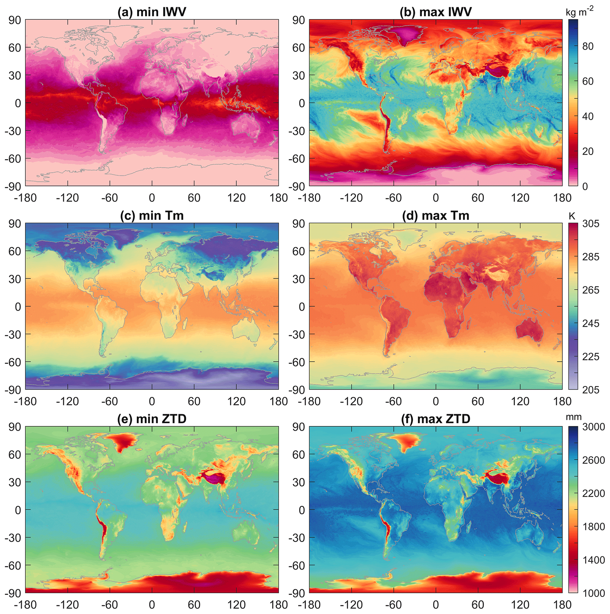
Figure A1Minima (a, c, e) and maxima (b, d, f) of IWV, Tm, and ZTD in 2020 obtained from the 1-hourly ERA5 surface level product.
The vertical coordinate of a GPS station estimated by GPS data processing is usually ellipsoidal height (Hel, in metre), which is the height above reference ellipsoid. By contrast, the geopotential altitude (i.e. geopotential height; Hgp) in units of geopotential metre (gpm) is referenced to mean sea level (MSL) and adjusted according to gravity variations. As Hgp is commonly used in meteorology (e.g. ERA5 and radiosonde), we converted Hel into Hgp for the GPS stations.
We first converted the reference of the GPS station's altitude from ellipsoid to MSL by using geoid model EGM2008 (Earth Gravitational Model 2008; Pavlis et al., 2012):
where the Hor and N are the orthometric and geoid heights in metre, respectively.
We then adjusted the altitude of the GPS station (with a latitude of φ) by considering gravity variations (World Meteorological Organization, 2018):
In the development of the enhanced GPS (enGPS) IWV product, the required GPS station pressure (Ps) and weighted mean temperature (Tm) were calculated from the temperature (T), relative humidity (RH), and geopotential height (H) from the ERA5 pressure level product.
Therefore, we first selected the four horizontally adjacent ERA5 grid nodes (i, i=1, 2, 3, 4) from the GPS station's location and then carried out vertical adjustments and horizontal interpolations. For each horizontally adjacent grid node, the vertical adjustment was conducted as follows. If the station altitude (Hs) is lower than the bottom ERA5 pressure level at the ith node, then the station pressure was estimated with the International Civil Aviation Organization's (ICAO) barometric correction formula:
where H0, P0, and T0 are the altitude, pressure, and temperature of the bottom ERA5 level at the ith node, and γ=0.0065 K m−1, g0=9.80665 m s−2, and Rd=287.033 J kg−1 K−1.
If Hs is between the jth and (j+1)th ERA5 levels, we first estimated the station pressure from both levels with Eq. (C1) separately with values of and . We then obtained the final adjusted station pressure by weighting of the two values (Schueler, 2001):
where and .
As shown in Eq. (4) in Sect. 2.3, Tm is dependent on the T and water vapour pressure (e) profiles from the station to the top. The e was estimated by using T and RH from ERA5:
where esat is saturation vapour pressure determined by Tetens' formula provided by the ECMWF's IFS Documentation CY45R1 (2018):
where a1=6.112 hPa and T0=273.16 K. If T≥T0 (over water), a3=17.502 and a4=32.19 K. If T≤Tice (250.16 K, over ice), a3=22.587 and K. If (mixed phase), the esat was estimated as a mix of those estimated over water and ice (esat(water) and esat(ice)):
In the end, we calculated the Ps and Tm by using a horizontal inverse distance weighted (IDW) interpolation of the estimates at the four grid nodes (Jade and Vijayan, 2008).
In situ meteorological observations were used to calculate Ps, Tm , and IWV at the GPS station in Sect. 4. For example, the Ps was estimated by using synoptic observations from the ISD dataset with Eq. (C1). The Tm was estimated with radiosonde observations from the IGRA dataset with Eq. (4) and Eqs. (C3)–(C5). The IGRA-derived IWV was calculated as follows:
where qj (in kg kg−1) and gj (in kg m−2) are the average specific humidity and local gravitational acceleration between the jth and (j+1)th levels from the station altitude to the top of the radiosonde profile. ΔHj is the altitude difference between the two adjacent levels. The specific humidity was calculated as below:
The local gravitational acceleration was calculated as a function of latitude (φ in rad) and orthometric altitude (Hor in m) given by (World Meteorological Organization, 2018)
NGL employs the gridded ZHD product provided by TUW at a single level and calculates the ZHD at GPS stations by using vertical adjustment as follows (Boehm et al., 2007; Kouba, 2008): (1) find the horizontally adjacent four grid nodes of a particular GPS station and extract their ZHD values at the Earth's surface from the TUW product, (2) convert the ZHD into pressure (P0) according to Eq. (4) at each node, (3) adjust the pressure from the altitudes of the surface (H0) to the GPS station (Hs) by using the barometric formula as follows:
(4) convert the pressure at the altitude of the station (Ps) over each grid node into the ZHD with Eq. (5) in Sect. 2.3, and (5) estimate the ZHD at the location of the GPS station with a horizontal interpolation.
The supplement related to this article is available online at: https://doi.org/10.5194/essd-15-723-2023-supplement.
PY: conceptualisation, methodology, formal analysis, investigation, writing – original draft, and visualisation. GB, CK, WCH, and DA: GPS ZTD product generation. XY and PY: IGRA and ISD data processing. RVM, MM, WJ, and JA: investigation and reviewing. HK: investigation, reviewing, supervision, project administration, and funding acquisition. All: manuscript editing.
The contact author has declared that none of the authors has any competing interests.
Publisher's note: Copernicus Publications remains neutral with regard to jurisdictional claims in published maps and institutional affiliations.
This article is part of the special issue “Analysis of atmospheric water vapour observations and their uncertainties for climate applications (ACP/AMT/ESSD/HESS inter-journal SI)”. It is not associated with a conference.
We are grateful to NGL for providing the GPS ZTD products and many institutions for sharing the continuous GPS observations. We also thank the ECMWF, TUW, and NCEI for providing the ERA5, TUW, IGRA radiosonde, and ISD synoptic data.
This work was funded at KIT with the German Research Foundation (DFG, project no. 321886779). This work was funded at NGL with NASA grants 80NSSC19K1044 and 80NSSC22K0463.
This paper was edited by David Carlson and reviewed by three anonymous referees.
Beirle, S., Lampel, J., Wang, Y., Mies, K., Dörner, S., Grossi, M., Loyola, D., Dehn, A., Danielczok, A., Schröder, M., and Wagner, T.: The ESA GOME-Evolution “Climate” water vapor product: a homogenized time series of H2O columns from GOME, SCIAMACHY, and GOME-2, Earth Syst. Sci. Data, 10, 449–468, https://doi.org/10.5194/essd-10-449-2018, 2018.
Bertiger, W., Bar-Sever, Y., Dorsey, A., Haines, B., Harvey, N., Hemberger, D., Heflin, M., Lu, W., Miller, M., Moore, A. W., Murphy, D., Ries, P., Romans, L., Sibois, A., Sibthorpe, A., Szilagyi, B., Vallisneri, M., and Willis, P.: GipsyX/RTGx, a new tool set for space geodetic operations and research, Adv. Space Res., 66, 469–489, https://doi.org/10.1016/j.asr.2020.04.015, 2020.
Bevis, M., Businger, S., Herring, T., Rocken, C., Anthes, R., and Ware, R.: GPS Meteorology: Remote Sensing of Atmospheric Water Vapor Using the Global Positioning System, J. Geophys. Res.-Atmos., 97, 15787–15801, https://doi.org/10.1029/92JD01517, 1992.
Bevis, M., Businger, S., Chiswell, S., Herring, T. A., Anthes, R. A., Rocken, C., and Ware, R. H.: GPS Meteorology: Mapping Zenith Wet Delays onto Precipitable Water, J. Appl. Meteorol., 33, 379–386, https://doi.org/10.1175/1520-0450(1994)033<0379:GMMZWD>2.0.CO;2, 1994.
Blewitt, G., Hammond, W. C., and Kreemer, C.: Harnessing the GPS data explosion for interdisciplinary science, Eos, 99, 485, https://doi.org/10.1029/2018EO104623, 2018.
Bock, O.: Standardization of ZTD screening and IWV conversion, in: Advanced GNSS Tropospheric Products for Monitoring Severe Weather Events and Climate: COST Action ES1206 Final Action Dissemination Report, edited by: Jones, J., Guerova, G., Douša, J., Dick, G., de Haan, S., Pottiaux, E., Bock, O., Pacione, R., and Van Malderen, R., Springer International Publishing, 314–324, https://doi.org/10.1007/978-3-030-13901-8, 2020.
Bock, O., Bosser, P., Pacione, R., Nuret, M., Fourrié, N., and Parracho, A.: A high-quality reprocessed ground-based GPS dataset for atmospheric process studies, radiosonde and model evaluation, and reanalysis of HyMeX Special Observing Period, Q. J. Roy. Meteorol. Soc., 142, 56–71, https://doi.org/10.1002/qj.2701, 2016.
Bock, O., Bosser, P., Flamant, C., Doerflinger, E., Jansen, F., Fages, R., Bony, S., and Schnitt, S.: Integrated water vapour observations in the Caribbean arc from a network of ground-based GNSS receivers during EUREC4A, Earth Syst. Sci. Data, 13, 2407–2436, https://doi.org/10.5194/essd-13-2407-2021, 2021.
Boehm, J., Werl, B., and Schuh, H.: Troposphere mapping functions for GPS and very long baseline interferometry from European Centre for Medium-Range Weather Forecasts operational analysis data, J. Geophys. Res.-Solid, 111, B02406, https://doi.org/10.1029/2005JB003629, 2006.
Boehm, J., Heinkelmann, R., and Schuh, H.: Short Note: A global model of pressure and temperature for geodetic applications, J. Geod., 81, 679–683, https://doi.org/10.1007/s00190-007-0135-3, 2007.
CY45R1 – Part IV: Physical processes, IFS Documentation CY45R1, https://doi.org/10.21957/4whwo8jw0, 2018.
Davis, J. L., Herring, T. A., Shapiro, I. I., Rogers, A. E. E., and Elgered, G.: Geodesy by radio interferometry: Effects of atmospheric modeling errors on estimates of baseline length, Radio Sci., 20, 1593–1607, https://doi.org/10.1029/RS020i006p01593, 1985.
Dee, D.: ECMWF reanalyses: Diagnosis and application, in: ECMWF Seminar on Diagnosis of Forecasting and Data Assimilation Systems, 7–10 September 2009, Reading, UK, https://www.ecmwf.int/sites/default/files/elibrary/2010/8931-ecmwf-reanalyses-diagnosis-and-application.pdf (last access: 27 January 2023), 2009.
Durre, I., Yin, X., Vose, R. S., Applequist, S., and Arnfield, J.: Enhancing the Data Coverage in the Integrated Global Radiosonde Archive, J. Atmos. Ocean. Tech., 35, 1753–1770, https://doi.org/10.1175/JTECH-D-17-0223.1, 2018.
ECMWF, ERA5 hourly data on pressure levels from 1959 to present, https://cds.climate.copernicus.eu, last access: 27 January 2023.
Ferreira, A. P., Nieto, R., and Gimeno, L.: Completeness of radiosonde humidity observations based on the Integrated Global Radiosonde Archive, Earth Syst. Sci. Data, 11, 603–627, https://doi.org/10.5194/essd-11-603-2019, 2019.
Fersch, B., Wagner, A., Kamm, B., Shehaj, E., Schenk, A., Yuan, P., Geiger, A., Moeller, G., Heck, B., Hinz, S., Kutterer, H., and Kunstmann, H.: Tropospheric water vapor: a comprehensive high-resolution data collection for the transnational Upper Rhine Graben region , Earth Syst. Sci. Data, 14, 5287–5307, https://doi.org/10.5194/essd-14-5287-2022, 2022.
Heise, S., Dick, G., Gendt, G., Schmidt, T., and Wickert, J.: Integrated water vapor from IGS ground-based GPS observations: initial results from a global 5-min data set, Ann. Geophys., 27, 2851–2859, https://doi.org/10.5194/angeo-27-2851-2009, 2009.
Hersbach, H., Bell, B., Berrisford, P., Hirahara, S., Horányi, A., Muñoz-Sabater, J., Nicolas, J., Peubey, C., Radu, R., Schepers, D., Simmons, A., Soci, C., Abdalla, S., Abellan, X., Balsamo, G., Bechtold, P., Biavati, G., Bidlot, J., Bonavita, M., Chiara, G. D., Dahlgren, P., Dee, D., Diamantakis, M., Dragani, R., Flemming, J., Forbes, R., Fuentes, M., Geer, A., Haimberger, L., Healy, S., Hogan, R. J., Hólm, E., Janisková, M., Keeley, S., Laloyaux, P., Lopez, P., Lupu, C., Radnoti, G., Rosnay, P. de, Rozum, I., Vamborg, F., Villaume, S., and Thépaut, J.-N.: The ERA5 global reanalysis, Q. J. Roy. Meteorol. Soc., 146, 1999–2049, https://doi.org/10.1002/qj.3803, 2020.
Jade, S. and Vijayan, M. S. M.: GPS-based atmospheric precipitable water vapor estimation using meteorological parameters interpolated from NCEP global reanalysis data, J. Geophys. Res.-Atmos., 113, D03106, https://doi.org/10.1029/2007JD008758, 2008.
Jiang, W., Yuan, P., Chen, H., Cai, J., Li, Z., Chao, N., and Sneeuw, N.: Annual variations of monsoon and drought detected by GPS: A case study in Yunnan, China, Sci. Rep., 7, 5874, https://doi.org/10.1038/s41598-017-06095-1, 2017.
Jin, S., Li, Z., and Cho, J.: Integrated Water Vapor Field and Multiscale Variations over China from GPS Measurements, J. Appl. Meteorol. Clim., 47, 3008–3015, https://doi.org/10.1175/2008JAMC1920.1, 2008.
Jones, J., Guerova, G., Douša, J., Dick, G., de Haan, S., Pottiaux, E., Bock, O., Pacione, R., and van Malderen, R. (Eds.): Advanced GNSS Tropospheric Products for Monitoring Severe Weather Events and Climate: COST Action ES1206 Final Action Dissemination Report, Springer International Publishing, Cham, https://doi.org/0.1007/978-3-030-13901-8, 2020.
Karl, T. R. and Trenberth, K. E.: Modern Global Climate Change, Science, 302, 1719–1723, https://doi.org/10.1126/science.1090228, 2003.
Kestin, J., Sengers, J. V., Kamgar-Parsi, B., and Sengers, J. M. H. L.: Thermophysical Properties of Fluid H2O, J. Phys. Chem. Ref. Data, 13, 175–183, https://doi.org/10.1063/1.555707, 1984.
Kouba, J.: Implementation and testing of the gridded Vienna Mapping Function 1 (VMF1), J. Geod., 82, 193–205, https://doi.org/10.1007/s00190-007-0170-0, 2008.
Lindstrot, R., Stengel, M., Schröder, M., Fischer, J., Preusker, R., Schneider, N., Steenbergen, T., and Bojkov, B. R.: A global climatology of total columnar water vapour from SSM/I and MERIS, Earth Syst. Sci. Data, 6, 221–233, https://doi.org/10.5194/essd-6-221-2014, 2014.
Masson-Delmotte, V., Zhai, P., Pirani, A., Connors, S. L., Péan, C., Berger, S., Caud, N., Chen, Y., Goldfarb, L., and Gomis, M. I.: Climate Change 2021: The Physical Science Basis, in: Contribution of Working Group I to the Sixth Assessment Report of the Intergovernmental Panel on Climate Change, IPCC, Geneva, Switzerland, https://doi.org/10.1017/9781009157896, 2021.
NCEI: Integrated Global Radiosonde Archive (IGRA) Version 2, NCEI [data set], https://www.ncei.noaa.gov/access/metadata/landing-page/bin/iso?id=gov.noaa.ncdc:C00975 (last access: 27 January 2023), 2023a.
NCEI: Global Hourly – Integrated Surface Database (ISD), https://www.ncei.noaa.gov/products/land-based-station/integrated-surface-database (last access: 27 January 2023), 2023b.
NGL: Troposheric Products from Nevada Geodetic Lab (NGL), http://geodesy.unr.edu, last access: 27 January 2023.
Pacione, R., Araszkiewicz, A., Brockmann, E., and Dousa, J.: EPN-Repro2: A reference GNSS tropospheric data set over Europe, Atmos. Meas. Tech., 10, 1689–1705, https://doi.org/10.5194/amt-10-1689-2017, 2017.
Pavlis, N. K., Holmes, S. A., Kenyon, S. C., and Factor, J. K.: The development and evaluation of the Earth Gravitational Model 2008 (EGM2008), J. Geophys. Res.-Solid, 117, B04406, https://doi.org/10.1029/2011JB008916, 2012.
Petit, G. and Luzum, B. (Eds.): IERS Conventions (2010), IERS Technical Note 36, Verlag des Bundesamts für Kartographie und Geodäsie, Frankfurt am Main, 179 pp., ISBN 3-89888-989-6, 2010.
Saastamoinen, J.: Atmospheric correction for the troposphere and stratosphere in radio ranging of satellites, in: The use of artificial Satellites for geodesy, in: Geophysical Monograph 15, AGU, USA, 247–251, https://doi.org/10.1029/GM015p0247, 1972.
Schmid, R., Steigenberger, P., Gendt, G., Ge, M., and Rothacher, M.: Generation of a consistent absolute phase-center correction model for GPS receiver and satellite antennas, J. Geod., 81, 781–798, https://doi.org/10.1007/s00190-007-0148-y, 2007.
Schröder, M., Lockhoff, M., Fell, F., Forsythe, J., Trent, T., Bennartz, R., Borbas, E., Bosilovich, M. G., Castelli, E., Hersbach, H., Kachi, M., Kobayashi, S., Kursinski, E. R., Loyola, D., Mears, C., Preusker, R., Rossow, W. B., and Saha, S.: The GEWEX Water Vapor Assessment archive of water vapour products from satellite observations and reanalyses, Earth Syst. Sci. Data, 10, 1093–1117, https://doi.org/10.5194/essd-10-1093-2018, 2018.
Schueler, T.: On ground-based GPS tropospheric delay estimation, PhD Thesis, Univ. der Bundeswehr München, Fak. für Bauingenieur-und Vermessungswesen, Studiengang Geodäsie und Geoinformation, Munich, https://athene-forschung.unibw.de/doc/85240/85240.pdf (last access: 27 January 2023), 2001.
Smith, A., Lott, N., and Vose, R.: The Integrated Surface Database: Recent Developments and Partnerships, B. Am. Meteorol. Soc., 92, 704–708, https://doi.org/10.1175/2011BAMS3015.1, 2011.
Thébault, E., Finlay, C. C., Beggan, C. D., Alken, P., Aubert, J., Barrois, O., Bertrand, F., Bondar, T., Boness, A., Brocco, L., Canet, E., Chambodut, A., Chulliat, A., Coïsson, P., Civet, F., Du, A., Fournier, A., Fratter, I., Gillet, N., Hamilton, B., Hamoudi, M., Hulot, G., Jager, T., Korte, M., Kuang, W., Lalanne, X., Langlais, B., Léger, J.-M., Lesur, V., Lowes, F. J., Macmillan, S., Mandea, M., Manoj, C., Maus, S., Olsen, N., Petrov, V., Ridley, V., Rother, M., Sabaka, T. J., Saturnino, D., Schachtschneider, R., Sirol, O., Tangborn, A., Thomson, A., Tøffner-Clausen, L., Vigneron, P., Wardinski, I., and Zvereva, T.: International Geomagnetic Reference Field: the 12th generation, Earth Planets Space, 67, 79, https://doi.org/10.1186/s40623-015-0228-9, 2015.
Turato, B., Reale, O., and Siccardi, F.: Water Vapor Sources of the October 2000 Piedmont Flood, J. Hydrometeorol., 5, 693–712, https://doi.org/10.1175/1525-7541(2004)005<0693:WVSOTO>2.0.CO;2, 2004.
TUW: Vienna Mapping Functions Open Access Data, https://vmf.geo.tuwien.ac.at/, last access: 27 January 2023.
Upton, G. and Cook, I.: Understanding statistics, Oxford University Press, 672 pp., ISBN 10:0199143919, ISBN 13:978-0199143917, 1996.
Van Malderen, R., Brenot, H., Pottiaux, E., Beirle, S., Hermans, C., Mazière, M. D., Wagner, T., Backer, H. D., and Bruyninx, C.: A multi-site intercomparison of integrated water vapour observations for climate change analysis, Atmos. Meas. Tech., 7, 2487–2512, https://doi.org/10.5194/amt-7-2487-2014, 2014.
Vaquero-Martínez, J., Antón, M., Ortiz de Galisteo, J. P., Cachorro, V. E., Álvarez-Zapatero, P., Román, R., Loyola, D., Costa, M. J., Wang, H., Abad, G. G., and Noël, S.: Inter-comparison of integrated water vapor from satellite instruments using reference GPS data at the Iberian Peninsula, Remote Sens. Environ., 204, 729–740, https://doi.org/10.1016/j.rse.2017.09.028, 2018.
Vogelmann, H., Sussmann, R., Trickl, T., and Reichert, A.: Spatiotemporal variability of water vapor investigated using lidar and FTIR vertical soundings above the Zugspitze, Atmos. Chem. Phys., 15, 3135–3148, https://doi.org/10.5194/acp-15-3135-2015, 2015.
Wang, J. and Zhang, L.: Systematic Errors in Global Radiosonde Precipitable Water Data from Comparisons with Ground-Based GPS Measurements, J. Climate, 21, 2218–2238, https://doi.org/10.1175/2007JCLI1944.1, 2008.
Wang, J., Zhang, L., and Dai, A.: Global estimates of water-vapor-weighted mean temperature of the atmosphere for GPS applications, J. Geophys. Res.-Atmos., 110, D21101, https://doi.org/10.1029/2005JD006215, 2005.
Wang, J., Zhang, L., Dai, A., Hove, T. V., and Baelen, J. V.: A near-global, 2-hourly data set of atmospheric precipitable water from ground-based GPS measurements, J. Geophys. Res.-Atmos., 112, D11107, https://doi.org/10.1029/2006JD007529, 2007.
Worden, J., Noone, D., and Bowman, K.: Importance of rain evaporation and continental convection in the tropical water cycle, Nature, 445, 528–532, https://doi.org/10.1038/nature05508, 2007.
World Meteorological Organization: Guide to Instruments and Methods of Observation, Measurement of Meteorological Variables, WMO-No. 8, 397–398, ISBN 978-92-63-10008-5, 2018.
Yu, C., Li, Z., and Blewitt, G.: Global Comparisons of ERA5 and the Operational HRES Tropospheric Delay and Water Vapor Products with GPS and MODIS, Earth Space Sci., 8, e2020EA001417, https://doi.org/10.1029/2020EA001417, 2021.
Yuan, P., Hunegnaw, A., Alshawaf, F., Awange, J., Klos, A., Teferle, F. N., and Kutterer, H.: Feasibility of ERA5 integrated water vapor trends for climate change analysis in continental Europe: An evaluation with GPS (1994–2019) by considering statistical significance, Remote Sens. Environ., 260, 112416, https://doi.org/10.1016/j.rse.2021.112416, 2021.
Yuan, P., Blewitt, G., Kreemer, C., Hammond, W.C., Argus, D., Yin, X., Van Malderen, R., Mayer, M., Jiang, W., Awange, J., and Kutterer, H.: An enhanced integrated water vapour dataset from more than 10,000 global ground-based GPS stations in 2020, Zenodo [data set], https://doi.org/10.5281/zenodo.6973528, 2022.
Zhu, Y. and Newell, R. E.: Atmospheric rivers and bombs, Geophys. Res. Lett., 21, 1999–2002, https://doi.org/10.1029/94GL01710, 1994.
Zumberge, J., Heflin, M., Jefferson, D., Watkins, M., and Webb, F.: Precise point positioning for the efficient and robust analysis of GPS data from large networks, J. Geophys. Res.-Solid, 102, 5005–5017, 1997.
Zus, F., Deng, Z., and Wickert, J.: The impact of higher-order ionospheric effects on estimated tropospheric parameters in Precise Point Positioning, Radio Sci., 52, 963–971, https://doi.org/10.1002/2017RS006254, 2017.
- Abstract
- Introduction
- Data and methods
- Characterisations of the GPS IWV product
- Evaluation with in situ observations
- Evaluation of enGPS versus opGPS
- Data availability
- Summary and outlook
- Appendix A: Ranges of meteorological variables in 2020 from ERA5
- Appendix B: Geopotential altitude from ellipsoidal height
- Appendix C: Estimation of meteorological variables at GPS station
- Appendix D: Vertical adjustment of the ZHD in NGL's opGPS IWV product
- Author contributions
- Competing interests
- Disclaimer
- Special issue statement
- Acknowledgements
- Financial support
- Review statement
- References
- Supplement