Spatially resolved hourly traffic emission over megacity Delhi using advanced traffic flow data

This paper presents a bottom-up methodology to estimate multi-pollutant hourly gridded on-road traffic emission using advanced traffic flow and speed data for Delhi. We have used the globally adopted COPERT (Computer Programme to Calculate Emissions from Road Transport) emission functions to calculate the emission as a function of speed for 127 vehicle categories. At first, the traffic volume and congestion (travel time delay) relation is applied to model the 24 h traffic speed and flow for all the major road links of Delhi. The modelled traffic flow and speed shows an anti-correlation behaviour having peak traffic and emissions in morning–evening rush hours. We estimated an annual emission of 1.82 Gg for PM (particulate matter), 0.94 Gg for BC (black carbon), 0.75 Gg for OM (organic matter), 221 Gg for CO (carbon monoxide), 56 Gg for NO_x (oxides of nitrogen), 64 Gg for VOC (volatile organic compound), 0.28 Gg for NH₃ (ammonia), 0.26 Gg for N₂O (nitrous oxide) and 11.38 Gg for CH₄ (methane) for 2018 with an uncertainty of 60 %–68 %. The hourly emission variation shows bimodal peaks corresponding to morning and evening rush hours and congestion. The minimum emission rates are estimated in the early morning hours whereas the maximum emissions occurred during the evening hours. Inner Delhi is found to have higher emission flux because of higher road density and relatively lower average speed. Petrol vehicles dominate emission share (>50 %) across all pollutants except PM, BC and NO_x, and within them the 2W (two-wheeler motorcycles) are the major contributors. Diesel-fuelled vehicles contribute most of the PM emission. Diesel and CNG (compressed natural gas) vehicles have a substantial contribution in NO_x emission. This study provides very detailed spatiotemporal emission maps for megacity Delhi, which can be used in air quality models for developing suitable strategies to reduce the traffic-related pollution. Moreover, the developed methodology is a step forward in developing real-time emission with the growing availability of real-time traffic data. The complete dataset is publicly available on Zenodo at https://doi.org/10.5281/zenodo.6553770 (Singh et al., 2022).

1 Introduction

Exposure to vehicular emissions poses a greater risk to the air quality and human health (Lipfert and Wyzga, 2008; Salo et al., 2021; GBD 2021). On-road transport is the major contributor to the ambient air pollution and greenhouse gas emissions in urban areas, mainly near roads (Singh et al., 2014), therefore they are an important component of the local air quality management plans and policies (Gulia et al., 2015; DEFRA, 2016; NCAP, 2019; Sun et al., 2022). The actual traffic emission depends on several dynamic factors, such as emission factors, traffic volume, speed, vehicle age, road network and infrastructure, road type, fuel, driving behaviour, congestion etc. (Pinto et al., 2020; Jiang et al., 2021; Deng et al., 2020). Traffic emission modelling has evolved and improved over recent years, however gaps still exist because of the complexity and data involved in the emission inventory development. Moreover, the reliability of the emission decreases further when the emissions are spatially and temporally segregated (Super et al., 2020; Osses et al., 2021). There are differences in the reliability of emission inventories of developed and developing countries because of lack of space–time input data in developing countries (Pinto et al., 2020). The uncertainty associated with emission inventory is further propagated in air quality models making mitigation studies more challenging, mainly for developing countries such as India which is already facing air pollution issues (Pandey et al., 2021).

India is among the top 10 economies (sixth GDP rank) in the world in 2020 (GDP, 2020) and is recognized as a developing country. The population and economic growth have led to dense urbanization with poor air quality in cities (Ravindra et al., 2019; Liang and Gong, 2020; Singh et al., 2021). India hosts 22 cities among the top 30 polluted cities in the world (IQAIR, 2020). The national capital of India, Delhi, has pollution levels exceeding NAAQS and WHO guideline values (Singh et al., 2021). Earlier studies have estimated on-road traffic as the major local contributor to Delhi pollution (CPCB, 2011; Sharma and Dikshit, 2016) along with long-range transport sources associated with stubble burning and dust leading to severe pollution episodes (Liu et al., 2018; Bikkina et al., 2019; Ravindra et al., 2019; Beig et al., 2020; Singh et al., 2020).

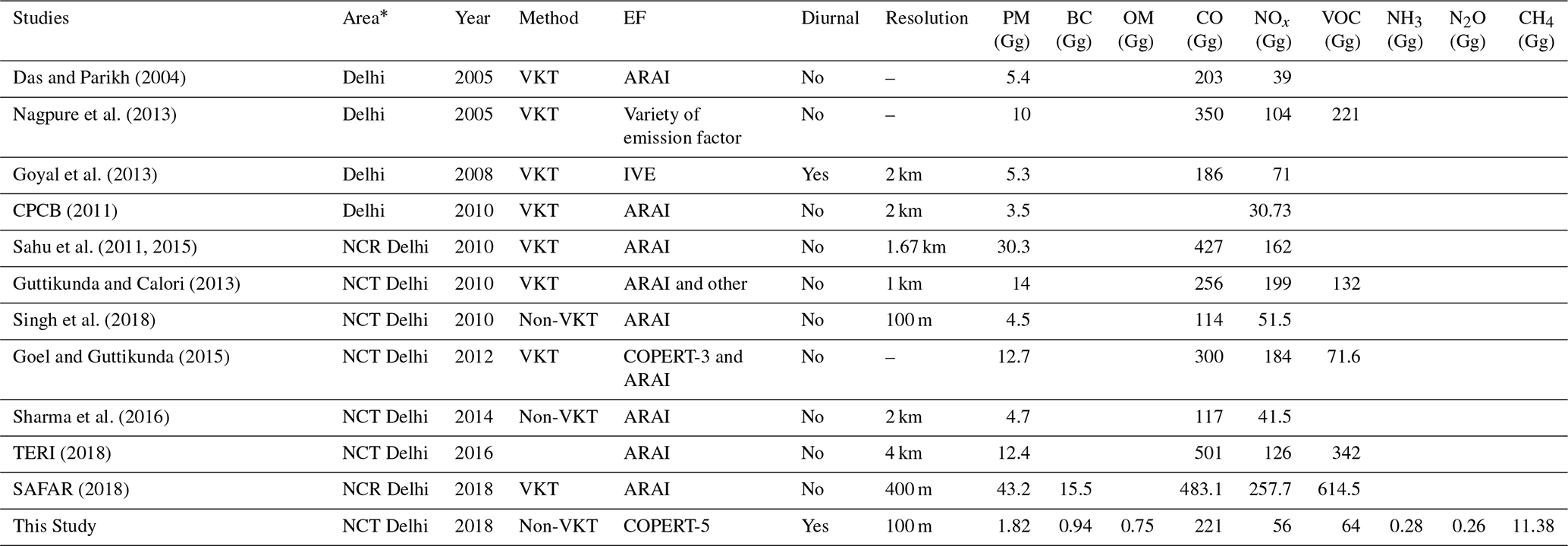
Delhi traffic exhaust (tailpipe) emissions have been studied extensively using different methodology for years. The emissions estimated by various studies show large variations (see comparison tables in Guttikunda and Calori, 2013; Goyal et al., 2013; Sharma et al., 2016; Singh et al., 2018, and in Table 6) suggesting that the emissions have large uncertainties associated with the method and data used. Most of the studies adopted a bottom-up methodology to calculate the total emission over Delhi based on the registered vehicles and average vehicle kilometres travelled (VKT) multiplied with emission factors. A few studies (e.g. Sharma et al., 2016; Singh et al., 2018, 2020) use an on-road traffic flow approach where emission is estimated for each line source (road link) then spatially segregated (Tsagatakis et al., 2020, Spatial emissions methodology). As per the study by the Central Pollution Control Board (CPCB, 2011), Goyal et al. (2013) further spatially desegregated the total emissions to 2 km × 2 km resolution, but the method of gridding is not discussed in detail. Sharma et al. (2016) and TERI (The Energy and Resources Institute, 2018) also estimated 2 km × 2 km and 4 km × 4 km gridded emission respectively, by adopting a per grid traffic flow method. Guttikunda and Calori (2013) estimated the 1 km × 1 km gridded emission by disaggregating the net emission using various spatial proxies like gridded road density. Though these studies with coarser resolution are helpful for identifying the emission hotspots, they lack actual traffic flow information disaggregated by road type and vehicle type within the grids. Moreover, their emission estimate shows large variations. For example, Das and Parikh (2004) and Nagpure et al. (2013) estimated traffic emission using VKT methodology for the same base year 2004, however their estimates varied by a factor of 2 or more. The annual emission estimate around year 2010 by CPCB (2011), Sahu et al. (2011, 2015), Goyal et al. (2013), Guttikunda and Calori (2013) and Singh et al. (2018) varied considerably from 3.5 Gg to ∼ 15 Gg for PM emission and 30 to 200 Gg for NO_x emissions. The VKT-based estimation approaches (Nagpure et al., 2013; Goel and Guttikunda, 2015; TERI, 2018) tend to estimate higher emission compared to the traffic flow methodology (Sharma et al., 2016; Singh et al., 2018). A 40 % increase in PM_2.5 emission in 2018 as compared to 2010 is reported by SAFAR (2018) and attributed to the increase in vehicular growth.

Most of the studies for Delhi use emission factors (EFs) developed by the Automotive Research Association of India (ARAI, 2008) and a few studies have used EFs from the international vehicular emission (IVE) model by USEPA (Davis et al., 2005) and the Computer Programme to Calculate Emissions from Road Transport (COPERT; Ntziachristos and Samaras, 2019). The ARAI EFs are measured under laboratory conditions, operating the vehicles in variable speed known as the Indian driving cycle (IDC, ARAI, 2008). The IVE emission factors are a function of the power bins of the vehicle engine, whereas in COPERT, emission factors are a function of average vehicle speed, vehicle technologies, estimated pollutants, correction methods, and adjustments to local conditions (Cifuentes et al., 2021). Goyal et al. (2013) used the IVE model to estimate the traffic emission over Delhi for the year 2008 and also studied the diurnal emission at a specific location. However, the study is limited to a fixed major traffic intersection only. Kumari et al. (2013) used the COPERT-3 emission factor to estimate emission for Indian cities, focusing on the multi-year (1991–2006) evolution of vehicular emission. However, this study estimates the total emissions based on registered vehicles and does not provide spatial segregation. The COPERT Tier-3 emissions have been used for comparison with real-world measured emission factors (Jaikumar et al., 2017; Choudhary and Gokhale, 2019). Jaikumar et al. (2017) identified vehicle idling as the major factor in the deviation between model-based estimation and measured emission as the vehicles spend 20 % of their time in idling mode.

The traffic volume and speed information over each road are vital for accurate emission estimation. The data over Delhi have been very limited; therefore, studies have used the VKT approach which uses the number of registered vehicles to estimate the emission. To the best of our knowledge, despite several studies for Delhi, none of the studies have studied Delhi emissions using advanced and detailed traffic data and speed based EFs to estimate the hourly gridded emissions at high resolution. Moreover, most of the studies are limited to the estimation of PM, NO_x, CO and HC only. The availability of recent detailed traffic data and speed volume relation (Malik et al., 2018, 2021) as a part of the Transportation Research and Injury Prevention Programme (TRIPP) of Indian Institute of Technology (IIT) Delhi provides an opportunity to estimate and improve the emissions over Delhi. To the best of our knowledge, this is the first study of its kind that considers advanced traffic flow data and estimates the hourly multi-pollutant emissions as a function of speed.

In this study, we have adopted a globally accepted methodology based on COPERT-5 Tier-3 to estimate the hourly gridded emission for Delhi at high resolution for 2018. COPERT EFs have been used in many studies, i.e. Álamos et al. (2022) for Chile, Mangones et al. (2019) for Bogota, Cifuentes et al. (2021) for Manizalesto, Wang et al. (2010) for Chinese cities, Vanhulsel et al. (2014) for Belgium, Tsagatakis et al. (2020) for the national emission inventory over the UK and many users around the globe. (https://www.emisia.com/utilities/copert/, EMISIA, 2021, last access: 10 October 2021). We combine advanced traffic volume and speed data (TRIPP; Malik et al., 2018) with speed-based emission factors to calculate the emissions. The methodology considers different vehicle types, fuel type, engine capacity, emission standard and other key parameters such as congestion to estimate the emission for each road. We estimate the emission of particulate and gaseous pollutants namely PM (particulate matter), BC (black carbon), OM (organic matter), CO (carbon monoxide), NO_x (oxides of nitrogen), VOC (volatile organic compound), NH₃ (ammonia) and greenhouse gases, N₂O (nitrous oxide) and CH₄ (methane). Most of the PM (∼ 98 %) from the vehicular exhaust is PM_2.5 (ARAI, 2008; Pant and Harrison 2013). We study the diurnal and spatial variability in the emission and identify the most polluting vehicle category, hotspots and the time when traffic emissions are highest. This study provides very detailed spatiotemporal emission maps for the megacity Delhi that can be used in air quality models for developing suitable strategies to reduce the traffic-related pollution. Moreover, the developed methodology is also a step forward in developing real-time emission models in the future with growing availability of real-time traffic data.

2 Methodology

We estimated the emissions for 2018 over the National Capital Territory (NCT) of Delhi having an area of 1483 km² (Fig. 1) and a population of 16.8 million (Census, 2011). The domain has been further divided into three regions (viz. inner, outer and east side), as shown in Fig. 1, to study the spatial variation in the emissions. Inner Delhi constitutes the major business hubs and workplaces within the ring road and the outer is the area away from the ring road, whereas the east side is the east part beyond the Yamuna River.

A bottom-up emission methodology has been adopted and a python-based model has been developed to estimate gridded hourly emissions of major pollutants over an urban area. The model estimates emission of PM, BC, OM, CO, NO_x, VOC, NH₃, N₂O and CH₄. The model uses hourly traffic activity and COPERT-based emission factors as a function of hourly speed for each road link across Delhi. The major vehicle categories include 2W (two-wheeler motor bikes), 3W (Auto rickshaws), CAR (passenger cars), BUS (buses), LCV (light commercial vehicles) and HCV (heavy commercial vehicles).

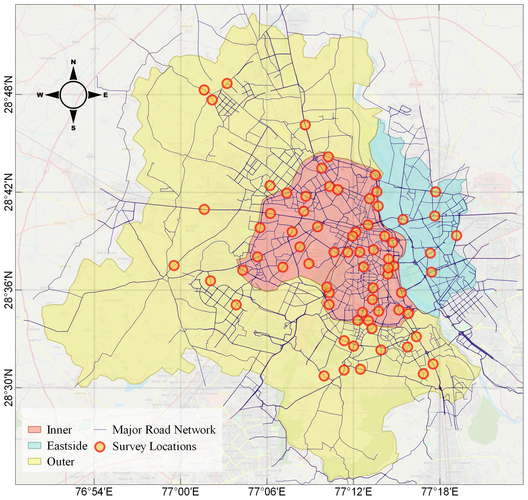
Figure 1 Map showing the study domain with TRIPP survey locations and the major road links over Delhi. The domain is segregated to three regions (Inner, East side and Outer) shown in different colours. The background map is from https://www.openstreetmap.org/ (last access: 1 December 2022); © OpenStreetMap contributors 2022. Distributed under the Open Data Commons Open Database License (ODbL) v1.0.

2.1 Traffic activity

Classified traffic volume and speed study of Delhi (Malik et al., 2018) provides traffic count and speed for the roads of Delhi based on the traffic volume and speed measurements conducted at 72 locations (Fig. 1) over Delhi in the year 2018 as a part of TRIPP of IIT Delhi. We will refer to this dataset as TRIPP data from now on. TRIPP data provide hourly traffic from 08:00–14:00 IST (Indian standard time) for eight fleet types (2W, 3W, cars, buses, minibuses, HCV, LCV and non-motorized vehicle; NMV) on more than 12 000 major road links over Delhi (Malik et al., 2018). These road links are further classified into five road classes (RClass1 to RClass5) based on the width of the road (Table S2). More detail of TRIPP traffic flow and its methodology is available elsewhere (Malik et al., 2018, 2021). As the TRIPP data are only available for 08:00–14:00 h, we use the speed–flow–density relationship by Malik et al. (2021) to estimate the hourly traffic for each road link in Delhi.

2.1.1 Generating traffic flow from congestion

The relation between traffic volume and congested speed has been studied extensively using the Greenshield model, the Greenberg model and the Underwood model (Wang et al., 2014; Hooper et al., 2014) and used by many studies (Jing et al., 2016; Yang et al., 2019) to estimate the traffic from the congestion for emission development. For Delhi, this relation is mathematically represented in Eq. (3) of Malik et al. (2021). By rearranging, the same can be written as Eq. (1) of this paper:

$$\begin{array}{}\text{(1)}& x_i=c_i{\left({\displaystyle \frac{\mathrm{1}}{\mathit{\alpha }}}\left({\displaystyle \frac{V_{o,i}}{V_{\mathrm{congested},i}}}-\mathrm{1}\right)\right)}^{\frac{\mathrm{1}}{\mathit{\beta }}},\end{array}$$

where x_i is traffic flow for road link i; c_i is traffic capacity for road link i; V_congested,i is speed during congestion (km h⁻¹) for link i; V_o,i is free flow velocity (FFV) of traffic for road link i; and α and β are constants (Table 1, Malik et al., 2021).

Traffic volume and road capacity determines the traffic speed. Increasing traffic volume leads to travel time delay (congestion) which further results in road traffic congestion, resulting in increased traffic volume and decreased speed leading to traffic delays. Congested traffic speed (V_congested) is inversely proportional to the congestion (Afrin and Yodo, 2020). Here, we define congestion as percentage increase in travel time, i.e. 50 % congestion level in a city means that a trip will take 50 % more time than it would during baseline uncongested conditions. In real-world situations, even with the light traffic, the congestion exists where minimum time delay is observed to reduce the likelihood of collision, known as single interaction (Vickrey, 1969). Therefore, the congestion cannot be zero in large cities such as Delhi with complex urban geometry and nighttime activity. Wei et al. (2022) reported lowest congestion value raging from 0.01 to 0.08 during nighttime across 77 Chinese cities. In this study, we have used hourly congestion data for Delhi obtained from TomTom (https://www.tomtom.com/en_gb/traffic-index/about/, last access: 10 October 2021). TomTom is one of the leading mapping and navigation services providing urban congestion worldwide. Congestion data have been taken for different days of the week, then combined to create weekdays (Monday to Friday) and weekend (Saturday and Sunday) profiles. Since FFV (V_o) and congestion are known for a road link, V_congested for weekdays and weekend has been calculated for each road link using the Eq. (2):

$$\begin{array}{}\text{(2)}& V_{\mathrm{congested}}={\displaystyle \frac{V_o}{\mathrm{1}+\mathrm{congestion}}}.\end{array}$$

Further, substituting the value of V_congested in Eq. (1), we get a relation between congestion and traffic flow (Eq. 3) that has been used to estimate the weekdays and weekend traffic flow for all the road links in personal car units (PCU):

$$\begin{array}{}\text{(3)}& x_i=c_i{\left({\displaystyle \frac{\mathrm{congestion}}{\mathit{\alpha }}}\right)}^{\frac{\mathrm{1}}{\mathit{\beta }}}\mathrm{congestion}>\mathrm{0}.\end{array}$$

For large cities such as Delhi, the nighttime congestion and traffic are not zero. It can be considered as a smooth traffic flow situation with congestion greater than zero. Therefore, to avoid zero traffic in Eq. (3), we have used a minimum congestion value of 0.03 (3 %) for Delhi. We use c_i from TRIPP and congestion from TomTom. The values α, β and c_i used in this study are taken from Malik et al. (2021), and are shown in Table S2. We take the three-point moving average of hourly congestion and calculate the traffic flow using Eq. (3). The traffic flow is calculated in terms of PCU. The PCU values for Delhi are taken from Malik et al. (2021) and are as follows: (a) 1.0 for CAR, (b) 0.5 for 2W, (c) 1.0 for 3W, (d) 3.0 for BUS, (e) 1.5 for LCV and (f) 3.0 for HCV. Malik et al. (2021) reported speed–volume relationships for different road classes in Delhi and provided these for different lanes (1 lane, 2 lanes, 3 lanes and >4 lanes). In order to harmonize the road classes, we use RClass1 for 1 lane, RClass2 for 2 lanes, RClass3 for 3 lanes, and RClass4 and RClass5 for >4 lanes. We selected the parameters of the road classes that have high numbers of sample points and R² corresponding to each road class. As an example, for RClass3, we considered the 3 lanes having higher R². Further, the speed and traffic volume has been corrected for each road link to match the observed PCU in TRIPP dataset for a better agreement. The PCU and speed variation across all road classes are shown as a box plot in Fig. S5. The comparison of observed and estimated traffic at the 72 locations of TRIPP is shown in Fig. S3. The estimated and measured traffic have a correlation of 0.99 and the difference (estimated − measured) varies from −0.6 % to 2.6 %. The hourly estimated traffic for each road link is further decomposed from PCU to different fleet categories using the percentage share provided by Malik et al. (2018). The hourly estimated traffic has been further corrected for the LCV and HCV using the percentage share provided by the Central Road Research Institute (CRRI; Errampalli et al., 2020) to account for the travel restrictions of good vehicles during peak traffic hours. For simplicity, the minibus category has been combined with the bus category and NMVs are not used in this study. To validate our activity data, the annual VKT estimated for each fleet category has been compared with earlier reported studies (Sahu et al., 2011; Kumar et al., 2011; Guttikunda and Calori, 2013; Goel et al., 2015; Malik et al., 2019) and is tabulated in Table S11 and discussed in Sect. 3.1.

2.2 Vehicular classification

The six types of primary vehicle categories (2W, 3W, CAR, BUS, LCV and HCV) have been further classified into 127 categories (Table S1) according to fuel, engine capacity and emission standards to match the COPERT-5 vehicular classification. The fuel share of petrol/gasoline, diesel and CNG (compressed natural gas)/LPG vehicles in Delhi for passenger and freight vehicles has been obtained from Dhyani and Sharma (2017) and Malik et al. (2019), respectively. The engine share for primary vehicle categories has been taken from working papers (Sharpe and Sathiamoorthy, 2019; Anup and Yang, 2020; Deo and Yang, 2020) of the International Council on Clean Transportation (ICCT). In India, the emission norms/standards, known as Bharat Stage (BS) which can be considered equivalent to the European emission standards – Euro, have been introduced in a phased manner. These norms were introduced for passenger cars and later extended to other vehicle categories. For example, the BS-I (India-2000) for passenger cars was implemented in 2000 followed by BS-II, BS-III and BS-IV in 2005, 2010 and 2017, respectively. The BS-VI for passenger cars has been recently introduced in 2020; therefore, it has not been considered in our study. For Delhi, the timeline of BS implementation for passenger cars and other vehicles are shown in Table S3. The vehicles prior to the implementation of BS norms have been considered as conventional (or BS-0 for simplicity). The BS share of the vehicles has been derived using the survival function method described in (Goel et al., 2015; Malik et al., 2019). The vehicle survival was calculated for the past 20 years by considering 2018 as the base year and then the BS share was calculated based on the age of the vehicle with respect to 2018 (Table S4). The final share of the primary vehicle category as per fuel, engine and BS norms has been calculated by multiplying the fuel share, engine share and BS norms share and shown in Table S1. In this study, BS and EURO/Euro have been used interchangeably, and BS-I to BS-IV, BS1 to BS4 or EURO1 to EURO4 represent the same emission standard.

2.3 Emission factors

The emission factor (EF) is a crucial parameter needed for emission estimation. Road traffic vehicular emission depends on a variety of factors such as vehicle type, fuel used, engine types, driving pattern, road type, emission legislation type (BS/EURO) and speed of the vehicle. We have adopted the recent COPERT-5 Tier-3 methodology and used the speed-based emission factor (https://www.emisia.com/utilities/copert/, EMISIA, 2021, last access: 10 October 2021) for 127 vehicle types (Table S1) and according to the emission legislation up to BS/EURO-4 (since BS-VI is not implemented in 2018). The EF as a function of vehicle speed (v) is calculated using Eq. (4):

$$\begin{array}{}\text{(4)}& \mathrm{EF}\left(v\right)={\displaystyle \frac{\left(\mathit{\alpha }\times v^{\mathrm{2}}\right)+\left(\mathit{\beta }\times v\right)+\mathit{\gamma }+\left(\frac{\mathit{\delta }}{v}\right)}{\left(\mathit{\epsilon }\times v^{\mathrm{2}}\right)+\left(\mathit{\zeta }\times v\right)+\mathit{\eta }}},\end{array}$$

where v is the speed and α, β, γ, δ, ε, ζ, and η are coefficients that vary with vehicle type.

The coefficients for each pollutant and vehicle category are taken from the COPERT-5 database (COPERT-5 guidebook, 2020). The emission factors are further corrected for the emission degradation occurring in older vehicles considering the mileage as discussed in the COPERT-5 guidebook (2020). COPERT relies on mean driving speed and travel distance. The mean speeds are relatively low under urban driving conditions, and emission factors are highly variable within this speed range due to the speed fluctuations caused due to real-time driving behaviour (frequent braking, acceleration, deceleration, idling). Lejri et al. (2018) have estimated the relative errors on fuel consumption and NO_x emissions related to mean speed variations from 2 to 10 km h⁻¹ and estimated errors up to 25 %–30 % in fuel consumption and NO_x emissions. Therefore, to account for the emissions due to the speed fluctuations around the mean speed, a factor of 1.2, i.e. 20 % increase has been applied to the final dataset. This has been applied for all the hours and all the pollutants. Although we apply the same factor for all hours of the day, the added emissions are more during high congestion hours and less during low congestion hours.

The non-exhaust emissions (Singh et al., 2020) have not been calculated in this study. As COPERT does not provide the EFs for the 3W CNG category, we have used EFs of CNG mini car for this. The BC and OM emissions are computed using the fraction (by COPERT-5 guidebook, 2020) from the PM exhaust. We have compared the COPERT EFs used in this study with the earlier reported EFs and shown in Table S12 to elaborate upon the potential uncertainty in the key vehicle categories. Further, the emission uncertainties have been discussed in Sect. 4.

2.4 Emission calculation

The model calculates hourly emissions for each road link of finite length and uses hourly traffic volume and emission factors as a function of speed for 127 vehicle categories (Table S1). The hourly emission rate (Q) for each road link is calculated using Eq. (5). The total emission for a given hour is calculated by taking the sum of emissions across all vehicle categories:

$$\begin{array}{}\text{(5)}& Q_{i,h}^p=\sum _j{V}_{i,j,h}\times {\mathrm{EF}}_j^p\left(v_{i,h}\right)\times L_i,\end{array}$$

where $Q_{i,h}^p$ is emission rate of a pollutant p for road link i and at hour h, where h=0 to 23; $V_{i,j,h}$ is the traffic volume of vehicle category j for road link i at hour h, where j=1 to 127; L_i is the length of road link i; and ${\mathrm{EF}}_j^p\left(v_{i,h}\right)$ is the emission factor of pollutant p for vehicle category j as a function of speed v_i,h for road link i at hour h.

The hourly emissions have been calculated for each pollutant over each road link then gridded at 100 m × 100 m resolution using the methodology described in Singh et al. (2018, 2020) to produce the hourly gridded emission inventory for Delhi.

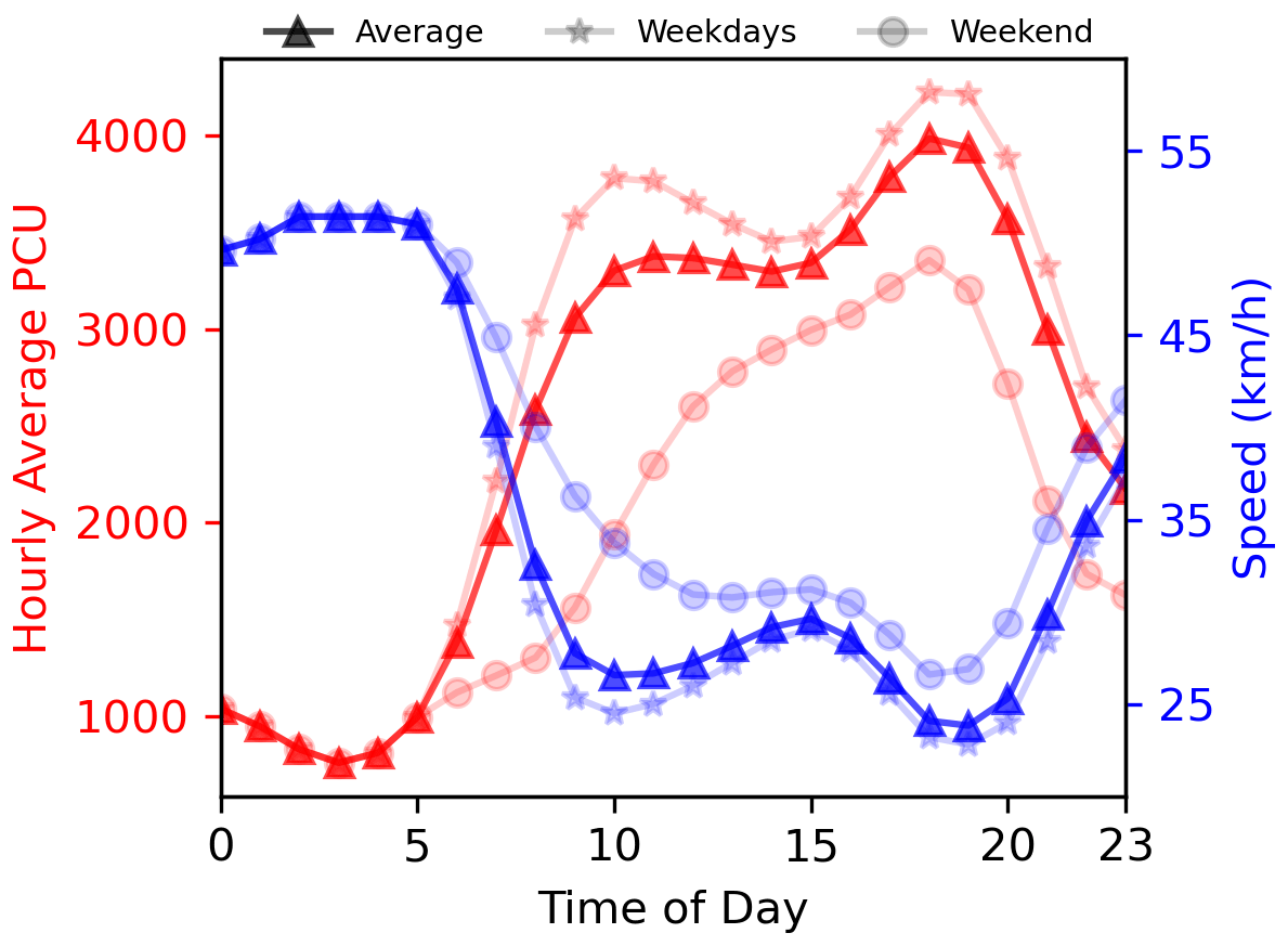
Figure 2 Weekdays, weekend and average diurnal profile for traffic volume in average PCU (red) and average speed (blue) over Delhi. The legend reflects the different markers used for weekdays, weekend and average profile.

3 Results

3.1 Diurnal variation of traffic volume and speed

The estimated hourly traffic volume (in PCU) and speed profiles for Delhi are shown in Fig. 2. An anticorrelated diurnal variation is seen in the traffic volume and speed. The traffic volume during weekdays tends to have a bimodal profile with a morning peak (09:00–11:00 IST) and an evening peak (18:00–20:00 IST). A similar traffic volume profile has also been observed by other studies over Delhi (Dhyani and Sharma, 2017; Sharma et al., 2019). Similar bimodal traffic profiles are also observed over the cities around the world subject to the city specific travel demand (Järvi et al., 2008 for Helsinki; Jing et al., 2016 for Beijing). The evening peak traffic volume tends to be 40 % higher than the morning peak. The vehicular composition changes hourly (Fig. S1) and also varies with respect to the road classes (Table S5). The nighttime goods vehicle share is more in comparison to the passenger and personal vehicles (Fig. S1). The weekend traffic volume does not show a morning peak due to closure of the offices/workplaces and shows evening peaks due to shopping and other weekend activities. As usual, the minimum traffic volume is observed at night (00:00–04:00 IST) because of the reduced human and commercial activities. Due to the minimum traffic at night, the traffic moves with an average speed of 51 ± 6 km h⁻¹ with almost no congestion. As traffic volume increases, it starts to build congestion, leading to reduced speed. The average speed during morning peak hours of the weekdays is estimated to be 30 ± 14 km h⁻¹, whereas the evening speed is estimated to be 28 ± 15 km h⁻¹. The evening congestion leads to an average 46 % reduction in the average speed, increasing the travel time by a factor of 2. We calculated the average profiles for each road link by combining weekdays and weekends and used them in the emission calculations. The estimated profiles averaged across all road links are shown in Fig. 2. We have estimated 27, 31, 6, 1.7, 0.95 and 3.14 billion VKT driven by CAR, 2W, 3W, BUS, HCV and LCV, respectively. The comparison between estimated annual VKT and reported by other studies is tabulated in Table S11. This comparison table includes the studies which have either reported annual VKT or have provided enough data to calculate annual VKT. The VKT values compare well with the earlier studies by considering the fact that the uncertainties exist in the method of estimation, year and study domain. Malik et al. (2019) estimated the destined and non-destined VKT of freight vehicles (HCV and LCV) with the actual measured traffic at several entry points in Delhi. Goel et al. (2015) estimated the annual VKT based on the annual mileage of the 2W and cars obtained from PUC (pollution under control) certification data and the number of registered vehicles. The VKT reported by Goel et al. (2015) for CARS and 2W are slightly lower than our study. The study by Goel et al. was conducted in 2012. Since then, the car and taxi share has almost doubled in Delhi due to increased travel demand and economic growth (DDA, 2021). The study by Kumar et al. (2011), which is for 2010, reported higher VKT for buses and HCV as compared to the one estimated by the current study. Their estimates were based on the assumed distance travelled by each vehicle and the number of registered vehicles than the actual on-road vehicle. Guttikunda and Calori (2013) reported high VKT for buses and HCV. The study by Sahu et al. (2011) for NCR Delhi estimated very high VKT for 2W and cars. While earlier studies have reported different VKT values, the relative VKT share compares well with our study. Moreover, the VKT estimated by recent studies are close to our estimates.

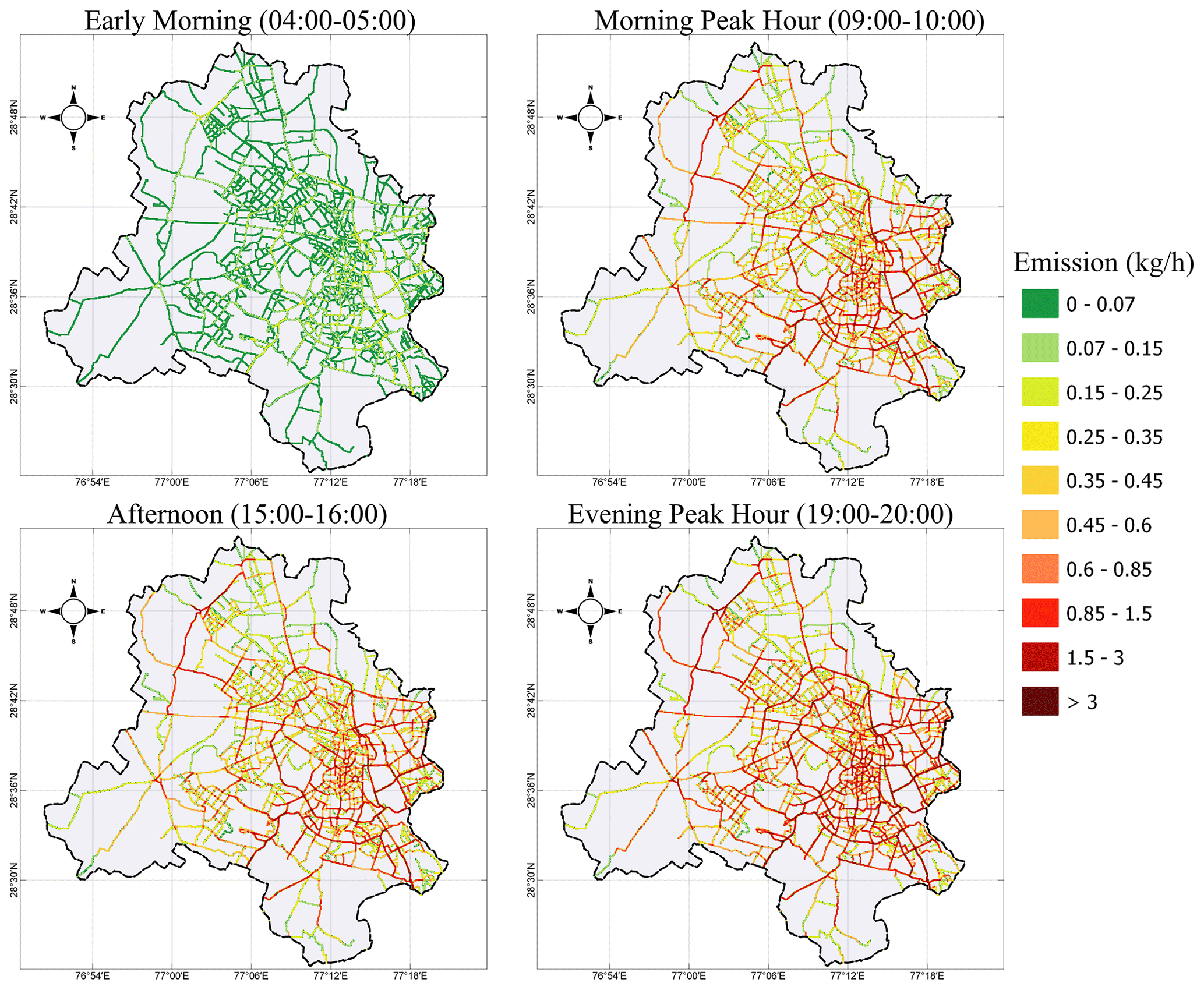
Figure 3 Estimated gridded NO_x emission in kg h⁻¹ (kilogram per hour) at 100 m × 100 m spatial resolution at different times of the day representative of different congestion levels.

3.2 Emission inventory

A multi-pollutant hourly and high spatial resolution (100 m × 100 m) emission inventory has been prepared for Delhi. As an example, the spatial distribution of NO_x emission at 03:00–04:00, 09:00–10:00, 15:00–16:00 and 18:00–19:00 IST, representing early morning, morning peak, afternoon and evening peak, respectively, is shown in Fig. 3. The emission rate during the evening peak hours is the highest during the day, followed by morning peak hours. The high traffic volume along with traffic congestions lead to more emissions during the peak traffic hours (Jing et al., 2016). The emission during the afternoon hours is comparable or less than that of the morning hours, whereas the early morning emissions are lowest because of low traffic volume moving with free flow speed. The diurnal profile of emissions has been discussed in detail in Sect. 3.5.

The annual emissions have been calculated by summing the hourly emissions to get daily emissions and then multiplying it with 365 (number of days in a year) to get annual emissions. The monthly variation in the emission has not been considered as the monthly variations are much smaller than the hourly variations. We estimated an annual emission of 1.82 Gg for PM, 0.94 Gg for BC, 0.75 Gg for OM, 221 Gg for CO, 56 Gg for NO_x, 64 Gg for VOC, 0.28 Gg for NH₃, 0.26 Gg for N₂O and 11.38 Gg for CH₄ in 2018.

3.3 Spatial variation

The hourly emissions over Delhi have been summed together to calculate the daily emissions for all the pollutants. The spatial variation of daily mean emission rate has been analysed over three selected regions, viz. inner, outer and east side Delhi  (as shown in Fig. 1). The total emission for each pollutant and for each region has been tabulated in Table S6. The outer Delhi region has the highest emission (51 %–53 %) for all the pollutants because of its largest area of 1106 km² which is 4.5 times of inner Delhi. To avoid the influence of area on the emissions, we have calculated the emission flux (i.e. emission per unit area) and shown in Table S7. The emissions flux is highest for inner Delhi, followed by east side and the outer Delhi region. For all pollutants, the emissions flux in inner Delhi is 40 %–50 % higher than the average emission of Delhi, whereas the emission flux in outer Delhi is ∼ 46 % lower. The emission flux is consistently high along the grids containing major roads (Fig. 3), intersections and major business hubs. Inner Delhi consists of major business hubs, workplaces and government offices, which entertain more vehicular activity in this region resulting in congestion that leads to reduced speed and enhanced emissions. The daytime average speed across all roads in inner Delhi is 29 km h⁻¹ which is lower than the daytime average speed of 32 km h⁻¹ in outer Delhi. The lower speed and higher traffic density influences the economic driving behaviour, resulting in frequent braking, idling, acceleration and deceleration that enhances the vehicular emission. Moreover, the morning and evening peak hours with higher traffic and lower speed have the highest emission as compared to the rest of the day. In these heavy congested hours, the vehicle is forced to run in lower speed which boosts the emission.

3.4 Emissions along the road class

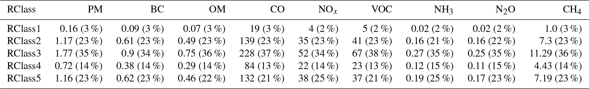
The emissions along the five road classes used in this study have been calculated and shown in Table 1, and the hourly variation of emission has been shown in Fig. 4. The RClass3 has a substantial emission share (∼ 35 %) across all pollutants followed by RClass5 and RClass2, whereas RClass1 holds the minimum emission share (∼ 2 %–3 %). The dominant emission share of RClass3 is due to the optimum vehicular activities over the longer road length. RClass2, which is the class of feeder roads to RClass3, RClass4 and RClass5, contributes ∼ 23 % to the emission. The multi-lane wider roads, RClass4 and RClass5, contribute ∼ 13 %–15 % and ∼ 21 %–25 % respectively to the total emission. To remove the dependency of the road length, we calculated the emission per kilometre segment of a road. The emissions (per km) over multi-lane wider roads (RClass4 and RClass5) are almost 2 times of the RClass3 (Table S8 and Fig. S2) due to more traffic flow, irrespective of the congested conditions. However, the emission per lane per kilometre (Table S9) for RClass1 is found to be the highest because of lower speed and congestion and major share of 2W. This shows that effective management of traffic in narrow roads to reduce the congestion will be beneficial in reducing the pollution without impacting the traffic volume. The multi-lane wider roads (RClass4 and RClass5) help the vehicle to maintain an economic speed resulting in minimum congestion and lower emission; however, they are the emission hotspots in Delhi.

Table 1 Emission in megagram (Mg) per day (% share) across different road types.

3.5 Diurnal variation of emission

Dynamic traffic volume and speed, as discussed in Sect. 3.1, results in diurnal variation in the emissions during a day. Figure 4 shows the hourly emissions (Mg h⁻¹) and contribution of each road class at each hour in Delhi. The temporal evolution of emission is linear with the traffic variation in a day with the minimum variation during the night-time and remarkable variation during the human active hours (08:00–20:00 IST). Among different road types and for all the pollutants, RClass1 has the lowest and RClass3 has the highest emission proportional to the traffic volume. A similar temporal variation of the NO_x emission rate is observed in a study, for different road types of Beijing (Jing et al., 2016). For most of the pollutants (except PM, BC and NO_x), daytime (08:00 to 20:00 IST) contributes ∼ 70 % to the daily emissions whereas the morning (09:00 to 11:00) and evening (18:00 to 20:00) rush hours alone altogether add 30 %–40 % to the total emissions. The increasing activity of goods vehicles (HCV + LCV) during afternoon and nighttime (Fig. S1) elevates the emission of PM, BC and NO_x from these vehicles (Fig. 5), resulting in a different diurnal profile compared to other pollutants. The emissions of NO_x and particulate pollutants (PM and BC) during late night hours (11:00–05:00 IST) is relatively higher, adding up to 60 % and 75 % of total particulate and NO_x nighttime emissions, respectively, as shown in Fig. 5. The contribution of vehicle type has been discussed in detail in Sect. 3.6. The diurnal evolution of emission is also visible in the hourly spatial map shown in Fig. 3. Early morning with minimum traffic volume has lower emission whereas the evening rush hour with increasing congestion has higher emission. The density of higher emission grids (Fig. 3) in the inner Delhi region is higher compared to other regions throughout the day.

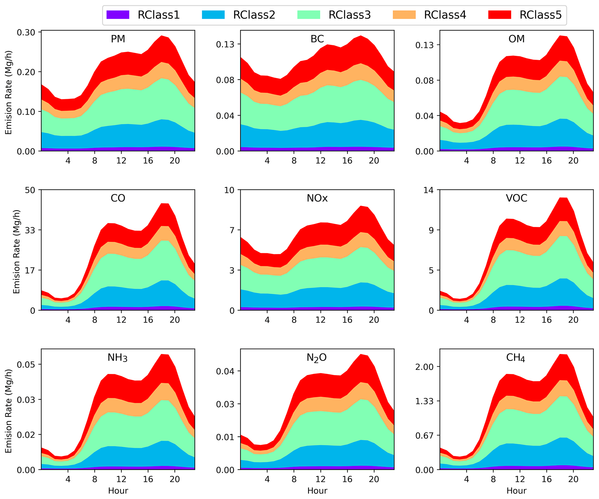
Figure 4 Variation of hourly emission (in Mg h⁻¹) of the nine pollutants averaged across Delhi according to the five road classes (RClass1 to RClass5). Different colours indicate the hourly contribution of each RClass to the total emission.

3.6 Vehicular emission share

The percentage share of major vehicle types to the total emission of nine pollutants has been calculated and shown in Table 2; and its hourly contribution is shown in Fig. 5. The 2W vehicles, having a major vehicular share (Table S5), are the major contributors to the total emissions for all the pollutants, except for BC, NO_x and N₂O. The goods vehicles (HCV and LCV) contribute substantially, mainly during nighttime, to the PM, BC and NO_x emissions. Buses have the highest contribution to NO_x emissions and substantial contribution to PM, BC and CH₄. Cars are the dominant source for NH₃ and N₂O and contribute substantially to PM, BC and NO_x emissions. However, most of the emissions are from diesel cars.

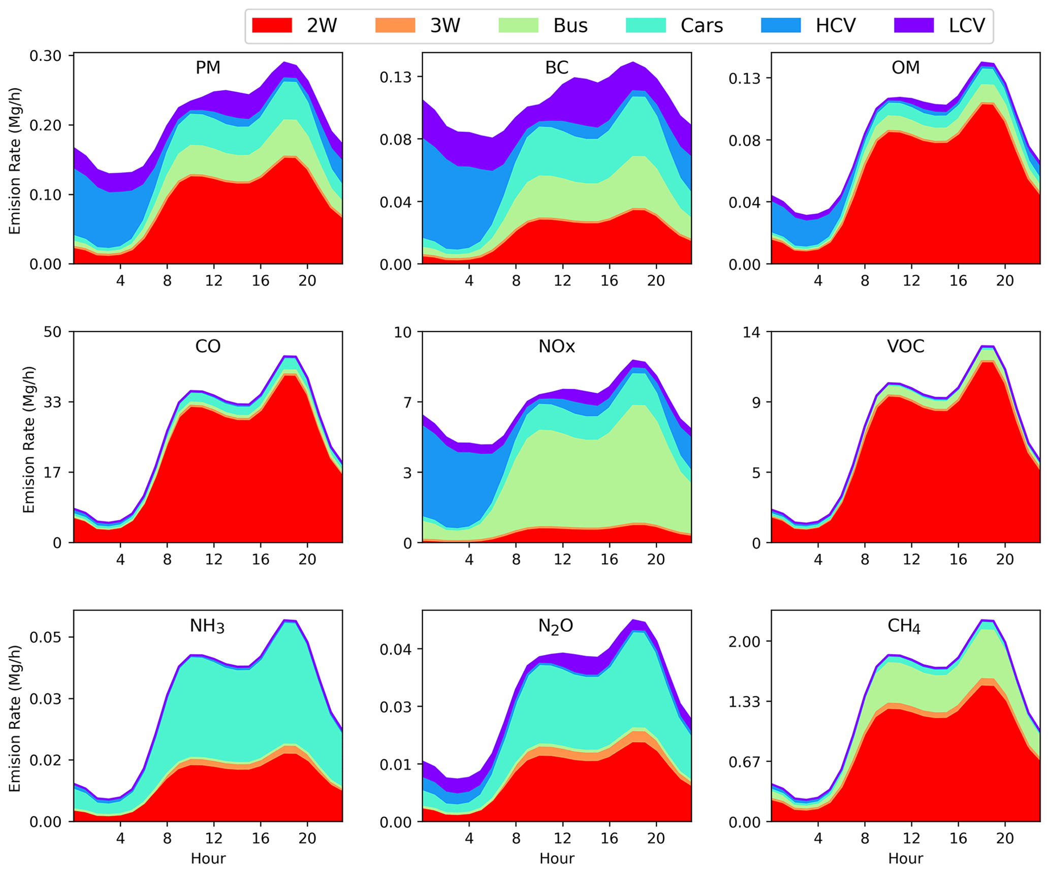
Figure 5 Variation of hourly emission (Mg h⁻¹) of the nine pollutants averaged across Delhi according to the major vehicle type. Different colours indicate the hourly contribution of each vehicle type to the total emission.

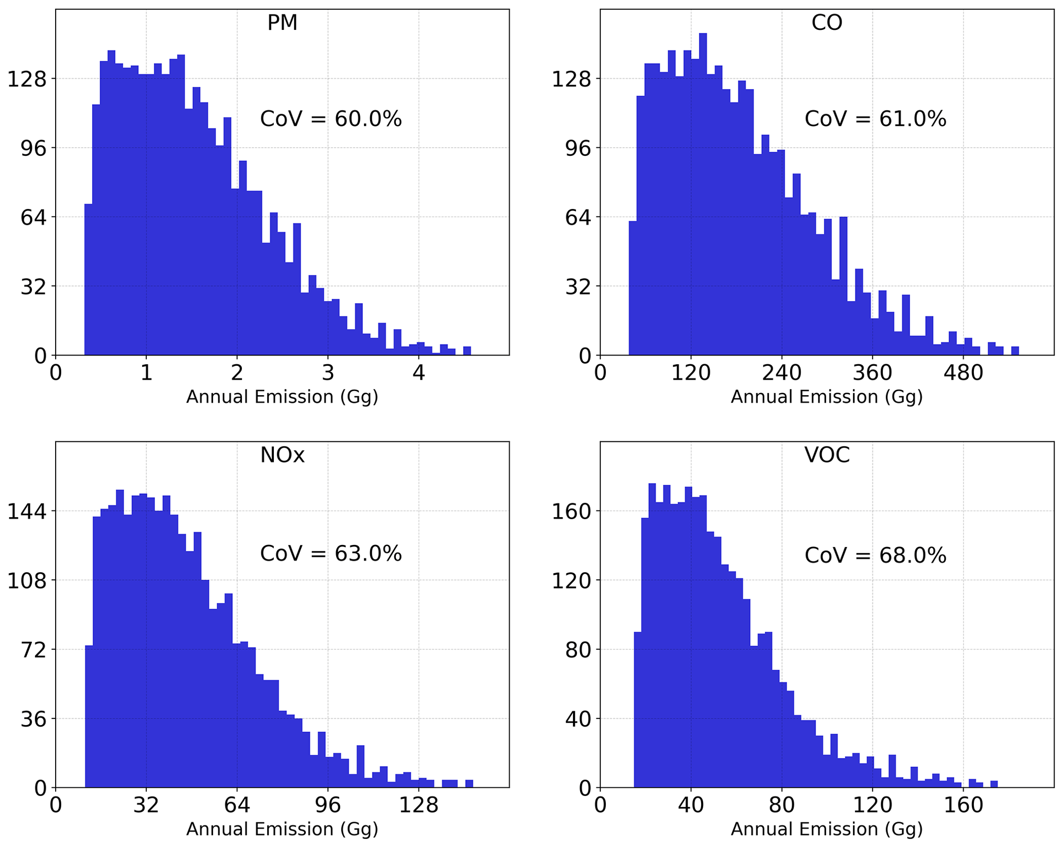
Figure 6 Histogram showing the variation in the annual emissions with the combination of sensitive parameters (VKT and EF).

Table 2 Emission in kg d⁻¹ (% share) according to the vehicle types.

Table 3 Emission in kg d⁻¹ (% share) according to fuel type.

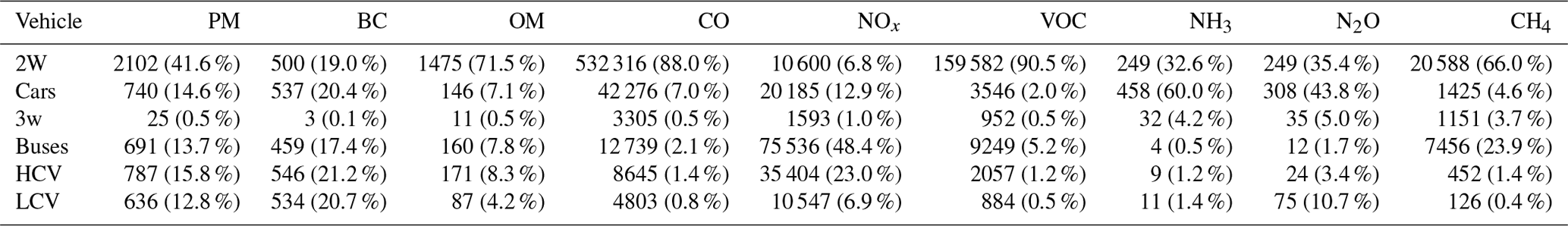
The vehicular fuel share to the total emission for each pollutant is shown in Table 3. Petrol vehicles are the largest contributors to the CO (∼ 94 %), VOC (91 %), NH₃ (86 %), OM (74 %), CH₄ (67 %) and N₂O (58 %), whereas diesel vehicles are the largest contributor to the BC (∼ 80 %), NO_x (59 %) and PM (54 %) emissions. The contribution of the CNG vehicles is relatively smaller, except for the NO_x and CH₄, where they contribute to ∼ 30 %, almost one third, of the total emissions. The larger contribution of petrol to the VOC, CO, OM and CH₄ emissions are dominated by 2W where we estimated that 2W in Delhi alone contribute 90 %, 88 %, 71 %, and 66 %, respectively, as shown in Table 2. The contribution of 2W is also highest to PM (42 %). The larger share of 2W towards the CO emissions has also been reported earlier, 61 % in Goyal et al. (2013); 43 % in Sharma et al. (2016) and 37 % in Singh et al. (2018). Higher emission share of 2W is due to the higher emission factor of VOC in petrol-fuelled 2W (Hakkim et al., 2021) that has also been reported in a multi-year emission study over Delhi by Goel and Guttikunda (2015). The PM emissions are dominated by diesel-fuelled HCVs (16 %), LCVs (13 %), buses (14 %) and cars (∼ 13 %), whereas 2W are the main source in petrol-fuelled vehicles contributing ∼ 42 % to the total PM emissions. Earlier, Sharma et al. (2016) reported 33 % share of 2W emissions in 2014. The share of petrol cars and CNG buses towards the PM, BC and OM emissions is less than 2 %. While it is clear that diesel-powered vehicles are the major source of PM emission, earlier studies have reported similar results but with large variations of HCVs in emission share. The largest share of diesel-fuelled HCV is reported as 92 % by Goyal et al. (2013), 46 % by Sharma et al. (2016) and 33 % by Singh et al. (2018). All these studies reported minimal emission share (less than 10 % combining both diesel and petrol cars). The largest share of HCV, LCV and diesel cars to BC emission is because of higher emission factors (Zavala et al., 2017) contributing to total urban BC emission as shown by Bond et al. (2013). The petrol cars contribute more than half of the total NH₃ emissions and among them, the Euro 2 with higher emission factor has the largest share of 39 %. The diesel vehicles (HCVs, LCVs, diesel buses and cars) altogether contribute significantly to the PM, BC and NO_x emissions. The higher emission factor of diesel-fuelled vehicles (Wu et al., 2012) clearly reflects in the emission share. The CNG buses have the highest share (27 %) in NO_x emission and around 23 % in CH₄ emissions. The highest share of CNG is due to the higher NO_x emission factor for CNG vehicles compared to petrol vehicles (Dimaratos et al., 2019). The larger share of ∼ 15 % from CNG buses to the total traffic NO_x emission is also reported in a study of CPCB (2011). In terms of Euro or BS standard, Euro 3 vehicles have the highest share (Table S10) in the total emission, except for N₂O and NH₃. This is mainly because of the highest share of Euro 3 vehicles in 2W, buses, HCV and LCV (Table S4 in the Supplement). In the case of N₂O, the emissions are dominated by Euro 4 cars which have around 84 % share to the total cars. For CH₄, the highest share of Euro 3 vehicles is due to the higher emissions from Euro 3 2W as the emission factor of petrol vehicles is higher (Clairotte et al., 2020).

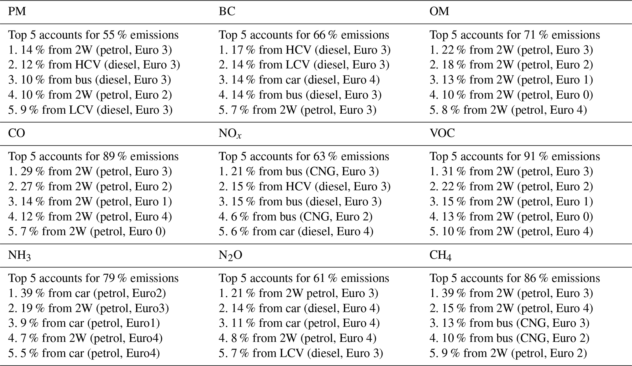
In order to have a clear picture of the dominant polluting vehicle categories, we grouped different vehicle types into 35 categories and calculated the percentage share to the total emission of 9 pollutants as shown in Table 4. We further identified the top five polluting vehicle categories for each pollutant and tabulated it in Table 5. For PM, the top five polluting vehicles account for 55 % of the total emissions, which is dominated by petrol Euro 3, petrol 2W and Euro 3 diesel HCVs. The BC emission is mainly driven by Euro 3 diesel HCVs, LCVs, buses and the top five polluting vehicles account for 66 % of the total emissions. The OM, CO, VOC emissions are dominated by 2W and the top five accounts for 71 %, 89 % and 91 % of total emissions, respectively. Petrol-fuelled cars and 2W hold the dominant share of NH₃ emissions because of the larger EF compared to other categories (COPERT-5 guidebook, 2020). For N₂O, 2W Euro 3 holds the highest share of 21 %, followed by EURO 4 diesel and petrol cars. The top five contributors to CH₄ emissions account for 86 % of the total emissions, which are dominated by 2W and CNG buses. These two categories of vehicles altogether contribute to ∼ 97 % of the emissions.

Table 4 Emission share of vehicles of different class, fuel and BS/EURO standards. Contributions less than 0.1 % are not shown here. Contributions more than 10 % are shown in the same colour. (D: diesel, P: petrol, C: CNG and number 0–4 represents the Euro type starting from 0 being conventional to 4 as Euro 4).

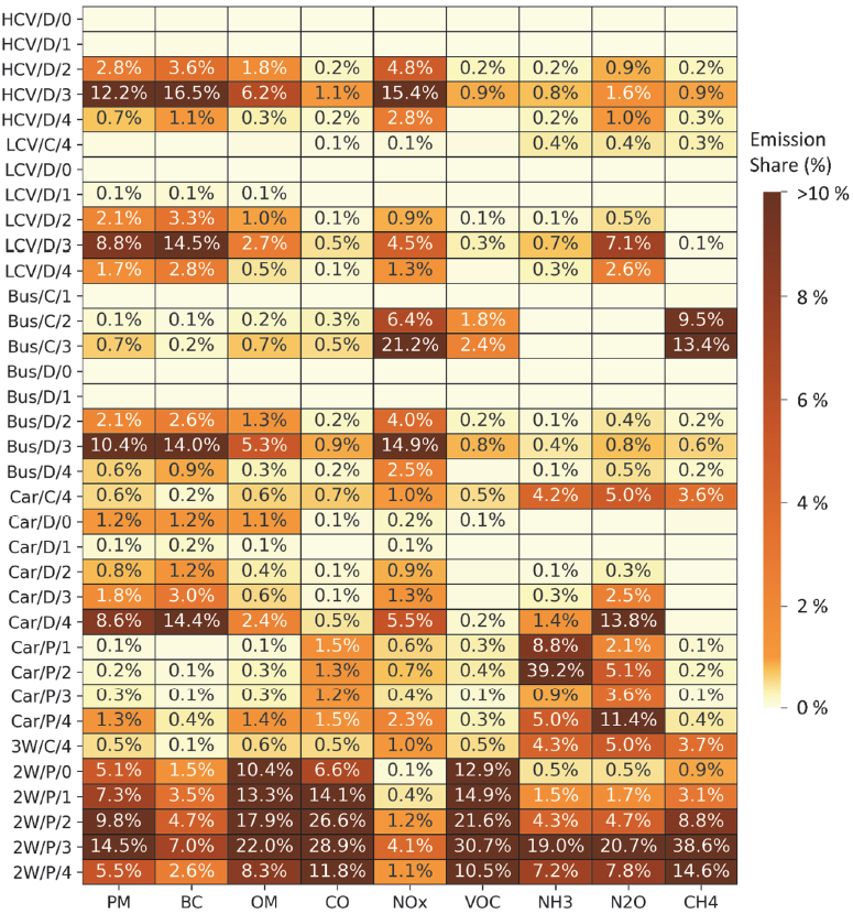
Table 5 Top five polluting vehicle categories for each pollutant.

4 Uncertainty in emissions

The emission uncertainty depends on the uncertainty of the model internal parameters (e.g. emission factors) and the uncertainty of the external parameters or input data (e.g. traffic activity, i.e. traffic volume and speed, distance travelled, vehicle category share, engine share, fuel share, technology share). Emissions are also influenced by environmental factors such as relative humidity and temperature (Kouridis et al., 2010; Dey et al., 2019). In most cases, model outputs are contingent on the accuracy of the input data. Because of the lack of very detailed spatiotemporal activity data, the calculated emissions are highly uncertain.

We have made an attempt to estimate the uncertainty in emissions of CO, PM, NO_x and VOC for which speed-based emission factors are available. We have calculated the uncertainty in the emissions by performing sensitivity analysis to VKT and EF. The VKT is a good proxy to represent the traffic activity. First, we estimated the uncertainty of ∼  40 % and ∼ 80 % in VKT and EF, respectively, based on the reported VKT and EF by earlier studies as shown in Tables S11 and S12, respectively. Then, we calculated the total emission of pollutants by varying the VKT from −40 % to +40 % of the VKT estimated by our study and by varying the EF from −80 % to +80 % with an interval of 10 %. The obtained distribution of the emission of pollutants is shown in Fig. 6. We calculated the coefficient of variation (CoV = [Std/ Mean] × 100 %) of the distribution and estimated an uncertainty of 61 %, 60 %, 63 % and 68 % for CO, PM, NO_x and VOC, respectively. Dey et al. (2019) estimated uncertainties of the emission of CO, VOC and NMVOC for Ireland in the range of −58 % to +76 %. Kouridis et al. (2010) estimated the coefficient of variation of 10 % for CO₂, in the order of 20 %–30 % for NO_x, VOC, PM_2.5, PM₁₀, 50 %–60 % for CO and CH₄ and over 100 % for N₂O.

Table 6 Traffic emission studies over Delhi.

^* NCT area is around 1483 km²; NCR area is around 4550 km².

5 Limitations

Geotagged dynamic traffic information and emission factors are the backbone of the emission inventory model. The traffic volume information is very crucial and traditionally obtained by manual counting or automated counters or through video surveillance at a few locations. However, in a real-world scenario, the traffic volume and speed can have large variations within a segment of a road. In this study, we have adopted the congestion-based approach (Jing et al., 2016; Yang et al., 2019) to model the traffic volume for each hour of the day. We use the same diurnal congestion profiles for all roads that could lead to emission uncertainty (Malik et al., 2021). In reality, some of the roads can be more congested than other roads based on the local population and traffic management.

The fleet composition can be different for different locations and at a given time of the day (Sharma et al., 2019). We have used the fleet composition based on surveyed composition at 72 locations during the daytime (08:00–14:00 IST) (TRIPP). To account for the peak hour and daytime entry restrictions of goods vehicles, we have used the share of goods vehicles (HCV and LCV) from the study by Errampalli et al. (2020). We use a constant share of fuel type, engine type and Euro type across all road links. The availability of detailed traffic data, though challenging, can improve the emission estimates.

Although the COPERT emission functions provide the speed-dependent emission factors for various classes of vehicles, they have been developed for European conditions. This adds to uncertainties while applying for Indian vehicles. The COPERT speed-dependent EFs are available only for the criteria pollutants such as PM, CO, NO_x and VOC. The emission factors used here are functions of average speed for each hour. These do not account for the emission errors due to the speed fluctuations caused due to real-time driving behaviour (frequent braking, acceleration, deceleration and idling) of the vehicles (Lejri et al., 2018; Lyu et al., 2021). We have tried to address these by adding another 20 % emission across all roads based on the earlier study (Lejri et al., 2018), however these could be uncertain but are within the range of uncertainty.

This study only focuses on the hot emissions and does not include cold start, evaporative emission. We do not consider change in the emissions due to the change in the ambient temperature and humidity (Franco et al., 2013). Additionally, we do not consider emissions associated with road slope, vehicle degradation and maintenance in detail. However, we have considered the vehicle degradation effect occurring in older vehicles considering the mileage as discussed in the COPERT-5 guidebook. Non-exhaust particulate matter emissions, such as dust resuspension, BW (brake wear), TW (tire wear) and RW (road wear) have not been considered in this study because of larger uncertainty. However, the non-exhaust emission of PM will be the dominant source of PM pollution in Delhi (Sharma et al., 2016; TERI, 2018; Singh et al., 2020). Residential roads, the small roads in residential areas, account for 80 % of the total length of Delhi, however their emission share has been reported to be only ∼ 3 % (Singh et al., 2018). We did not use these roads in our study, firstly, because of small share, secondly, we did not have a good quality data and thirdly, we wanted to optimize the computational cost.

We reported annual average emissions by considering traffic variations during weekdays and weekends (Fig. 2). We did not consider monthly variations as they are much smaller than the hourly variations. For example, the CoV of the EDGAR (Emissions Database for Global Atmospheric Research; Crippa et al., 2020) monthly emission data over Delhi (shown in Fig. S4) is around 2.5 %–3 % for CO, NMVOC (non-methane volatile organic compound), NO_x and PM_2.5, whereas we estimate hourly CoV of 54 %, 55 %, 19 % and 26 % for CO, VOC, NO_x and PM, respectively. We do consider the traffic variation of weekdays and weekends as they have substantial variations (Fig. 2). Moreover, the hourly congestion of weekends and weekdays from TomTom was available as annual mean for 2018; therefore, we estimated the annual average hourly emissions which were converted into annual emissions by summing the hourly emissions to get daily emissions and then multiplying them with 365.

The emissions estimated in this study for Delhi are comparable to the emissions estimated for other megacities. For example, road transport emission of NO_x and PM_2.5 for London was 20.8 and 1.12 Gg, respectively in 2016 (LAEI, 2016). The megacity Beijing, which has 3 times larger road network, had 4.1 Gg of traffic PM emission in 2013 (Jing et al., 2016). While our estimates are comparable to other megacities, these are lower as compared to the one reported by earlier studies for Delhi (Table 6). The lower emissions for Delhi can be expected because India has implemented the recent emission standards in a phased manner (Table S3) which should reflect in the traffic emission calculations. In many parts of the world, the road transport emission has decreased, despite an increase in transport vehicles, because of the improvements in engine technology (Winkler et al., 2018; Sun et al., 2019). One of the reasons for higher emission estimation by earlier studies for Delhi is the use of old EFs developed by ARAI way back in 2008. Therefore, these ARAI EFs tend to overestimate the emissions as it does not represent the recent emission standard technologies (i.e. Euro 3 and Euro 4). It is important to use recent emission factors such as COPERT-5 which can account for technology related emissions. Although we have considered advanced traffic flow data and estimated the hourly emission as a function of speed, the accuracy of the emissions is subject to quality of the input data and emission factors. Supplying a quality input data and removing ambiguity can improve the emission estimates and reduce the input data-related uncertainty.

6 Data availability

The emission dataset can be accessed through the open-access data repository https://doi.org/10.5281/zenodo.6553770 (Singh et al., 2022), under a CC BY-NC-ND 4.0 license. This dataset is presented as a netCDF covering the rectangular domain around the National Capital Territory (NCT) of Delhi. The data and analysis presented in the paper are only over the NCT area as shown in Fig. 3. TomTom-averaged congestion data are available online (https://www.tomtom.com/en_gb/traffic-index/new-delhi-traffic/, TomTom, 2021). COPERT-5 emission factors are obtained from the EMISIA online platform (https://www.emisia.com/utilities/copert/, EMISIA, 2021) of Aristotle University, Thessaloniki.

7 Conclusion

Here we present a methodology to estimate high-resolution spatially resolved hourly traffic emission over Delhi using advanced traffic flow and speed. We estimated the emissions of major pollutants, viz. PM, BC, OM, CO, NO_x, VOC, NH₃, N₂O and CH₄.

We have used traffic volume and speed measurements conducted at 72 locations over Delhi in the year 2018 as a part of TRIPP of IIT Delhi. Additionally, we have used the hourly congestion data from TomTom to account for hourly changes in the speed. The previously studied relation between traffic volume and speed has been utilized to generate the hourly traffic volume and speed profile for each road link. The vehicles have been classified into 127 categories according to vehicle type, fuel type, engine capacity and emission standard. The COPERT-5 emission functions of speed are applied at a micro level for each hour along each road link to calculate the emissions that account for congestion and spatial variation in emission. To the best of our knowledge, this is the first study of its kind that considers advanced traffic flow data and estimates the hourly multi-pollutant emissions as a function of speed. We make the following conclusions.

1. We estimated an annual emission of 1.82 Gg for PM, 0.94 Gg for BC, 0.75 Gg for OM, 221 Gg for CO, 56 Gg for NO_x, 64 Gg for VOC, 0.28 Gg for NH₃, 0.26 Gg for N₂O and 11.38 Gg for CH₄ in 2018. We estimated an uncertainty of 60 %–68 % in these emissions by adding 40 % uncertainty in VKT and 80 % uncertainty in EFs.

2. The modelled traffic volume (in PCU) and speed profiles show bimodal distribution exhibiting an anti-correlation behaviour. The traffic volume peaks during morning and evening rush hours, resulting in lower speed. There is a mild enhancement in speed during the afternoon due to the less traffic. During the early morning hours, the vehicles almost achieve the free flow speed.

3. The diurnal variation of emission of pollutants are like traffic variations and show distinct bimodal distribution with morning and dominant evening peaks for almost all pollutants. However, the difference in nighttime and daytime emissions are less for PM, BC and NO_x due to the enhanced share of goods vehicles during the nighttime. The goods vehicles significantly contribute to the nighttime emission in Delhi. These emissions along with unfavourable meteorology (e.g. lower PBL and wind speed) might help in sustained PM levels during the nighttime in Delhi.

4. In terms of the spatial distribution, the emissions are higher along the major roads and the emission hotspots are near the traffic junctions. The emission flux in inner Delhi is highest due to the higher road and traffic density and lower average speed. This is 40 %–50 % higher than the mean emission flux of Delhi. However, the total emission is higher for outer Delhi due to its larger area having a total road length more than inner Delhi.

5. According to the road classes (RClass1 to RClass5, from single lane to multi-lane roads), we find that RClass3 has the highest emission share due to the highest total road length. However, the emission per kilometre is highest over multi-lane wider roads (RClass4 and RClass5) that are almost 2 times the RClass3 because of high traffic volume. Moreover, the emission per lane per kilometre is highest for RClass1 because of lower speed and congestion. While the effective management of traffic in narrow roads could be beneficial, the multi-lane roads act as emission hotspots. An analysis of the choice of road width should be performed to achieve the optimum emission without increasing the pollution exposure near the roads.

6. Petrol vehicles contribute to over 50 % emission of OM, CO, VOC, NH₃, N₂O and CH₄ emissions. For OM, CO, VOC, N₂O and CH₄, the petrol share is dominated by 2W whereas for NH₃, share is dominated by petrol cars. The diesel vehicles are the dominant contributor to PM, BC and NO_x emission.

7. In terms of emission standards, Euro 3 vehicles contribute the highest to all pollutants followed by Euro 4, with an exception to NH₃, where Euro 2, mainly petrol cars, are the dominant source.

8. Among vehicle classes, the 2Ws contribute the most to the total emissions for all the pollutants except for BC, NO_x and N₂O. The diesel vehicles including goods vehicles (HCV and LCV) contribute substantially to the PM, BC and NO_x emissions. The goods vehicles have a dominant share in the nighttime emissions. CNG buses have the highest contribution to NO_x and CH₄ emissions whereas diesel buses have substantial contributions to PM emissions. Petrol cars are the dominant source for NH₃ whereas diesel cars contribute substantially to PM, BC and NO_x emissions. The contribution of petrol cars to the PM emission is less than 2 %.

9. For all the pollutants, the top five polluting vehicle categories account for more than half (55 %–91 %) of the emissions. The pollutants such as CO, VOC, CH₄ and OM have a distinct source such as 2W. However, the PM and BC have mixed sources including 2W and diesel vehicles. NO_x emissions are mainly due to CNG and diesel vehicles. NH₃ is mainly emitted from petrol and diesel cars and N₂O has mixed sources including 2W and cars.

This spatiotemporal emissions can be used in air quality models for developing suitable strategies to reduce the traffic-related pollution in the megacity Delhi. Moreover, the developed methodology is a step forward in developing real-time emission prediction in the future with growing availability of real-time traffic data.