Near-real-time CO₂ fluxes from CarbonTracker Europe for high-resolution atmospheric modeling

We present the CarbonTracker Europe High-Resolution (CTE-HR) system that estimates carbon dioxide (CO₂) exchange over Europe at high resolution (0.1 × 0.2^∘) and in near real time (about 2 months' latency). It includes a dynamic anthropogenic emission model, which uses easily available statistics on economic activity, energy use, and weather to generate anthropogenic emissions with dynamic time profiles at high spatial and temporal resolution (0.1×0.2^∘, hourly). Hourly net ecosystem productivity (NEP) calculated by the Simple Biosphere model Version 4 (SiB4) is driven by meteorology from the European Centre for Medium-Range Weather Forecasts (ECMWF) Reanalysis 5th Generation (ERA5) dataset. This NEP is downscaled to 0.1×0.2^∘ using the high-resolution Coordination of Information on the Environment (CORINE) land-cover map and combined with the Global Fire Assimilation System (GFAS) fire emissions to create terrestrial carbon fluxes. Ocean CO₂ fluxes are included in our product, based on Jena CarboScope ocean CO₂ fluxes, which are downscaled using wind speed and temperature. Jointly, these flux estimates enable modeling of atmospheric CO₂ mole fractions over Europe.

We assess the skill of the CTE-HR CO₂ fluxes (a) to reproduce observed anomalies in biospheric fluxes and atmospheric CO₂ mole fractions during the 2018 European drought, (b) to capture the reduction of anthropogenic emissions due to COVID-19 lockdowns, (c) to match mole fraction observations at Integrated Carbon Observation System (ICOS) sites across Europe after atmospheric transport with the Transport Model, version 5 (TM5) and the Stochastic Time-Inverted Lagrangian Transport (STILT), driven by ECMWF-IFS, and (d) to capture the magnitude and variability of measured CO₂ fluxes in the city center of Amsterdam (the Netherlands).

We show that CTE-HR fluxes reproduce large-scale flux anomalies reported in previous studies for both biospheric fluxes (drought of 2018) and anthropogenic emissions (COVID-19 pandemic in 2020). After applying transport of emitted CO₂, the CTE-HR fluxes have lower median root mean square errors (RMSEs) relative to mole fraction observations than fluxes from a non-informed flux estimate, in which biosphere fluxes are scaled to match the global growth rate of CO₂ (poor person's inversion). RMSEs are close to those of the reanalysis with the CTE data assimilation system. This is encouraging given that CTE-HR fluxes did not profit from the weekly assimilation of CO₂ observations as in CTE.

We furthermore compare CO₂ concentration observations at the Dutch Lutjewad coastal tower with high-resolution STILT transport to show that the high-resolution fluxes manifest variability due to different emission sectors in summer and winter. Interestingly, in periods where synoptic-scale transport variability dominates CO₂ concentration variations, the CTE-HR fluxes perform similarly to low-resolution fluxes (5–10× coarsened). The remaining 10 % of the simulated CO₂ mole fraction differs by >2 ppm between the low-resolution and high-resolution flux representation and is clearly associated with coherent structures (“plumes”) originating from emission hotspots such as power plants. We therefore note that the added resolution of our product will matter most for very specific locations and times when used for atmospheric CO₂ modeling. Finally, in a densely populated region like the Amsterdam city center, our modeled fluxes underestimate the magnitude of measured eddy covariance fluxes but capture their substantial diurnal variations in summertime and wintertime well.

We conclude that our product is a promising tool for modeling the European carbon budget at a high resolution in near real time. The fluxes are freely available from the ICOS Carbon Portal (CC-BY-4.0) to be used for near-real-time monitoring and modeling, for example, as an a priori flux product in a CO₂ data assimilation system. The data are available at https://doi.org/10.18160/20Z1-AYJ2 (van der Woude, 2022a).

1 Introduction

Anthropogenic emissions of carbon dioxide (CO₂) increase atmospheric CO₂ mole fraction levels, which contribute strongly to the increase in global temperatures (Intergovernmental Panel on Climate Change, 2021). Responses of the climate system, including the rate of carbon exchange with the biosphere itself, are observed to change along with the unprecedented speed of CO₂ rise (Friedlingstein et al., 2022b). With that realization, a total of 196 parties have committed to the Paris Agreement, which aims to reduce anthropogenic greenhouse gas (GHG) emissions and to limit global warming to 2 ^∘C, but preferably 1.5 ^∘C. Ratification of the Paris Agreement requires each country to set specific goals to reduce anthropogenic GHG emissions in their National Determined Commitments (NDCs) and to support independent verification of national greenhouse gas inventories reported to the United Nations Framework Convention on Climate Change (UNFCCC).

To monitor progress towards the Paris Agreement goals and to verify reported greenhouse gas emissions, the EU is developing a monitoring and verification support (MVS) as part of their Copernicus program (Balsamo et al., 2021). The MVS is expected to heavily use observations of the carbon cycle from in situ and satellite platforms (Pinty et al., 2017; Janssens-Maenhout et al., 2021; Balsamo et al., 2021). Quantitative use of CO₂ (Breón et al., 2015; Boon et al., 2016; Wang et al., 2018; Nalini et al., 2022) and CH₄ (Bergamaschi et al., 2005; Henne et al., 2016; Thompson et al., 2022) mole fraction measurements or retrieval products in data assimilation (DA) systems can provide a so-called top-down view of the European carbon balance. In such a setup, the combination of reported or simulated GHG fluxes and atmospheric transport allows a continuous comparison to observations, and large discrepancies identify underestimated or overestimated surface fluxes. Successful implementations of this concept, e.g., for Switzerland for CH₄ (Henne et al., 2016), halocarbons (Brunner et al., 2017) and N₂ and CFC (Manning et al., 2011) emissions, have provided important feedback to their national emission registration entity (NER) that reports to the UNFCCC. From the MVS perspective, such efforts are best done operationally and in near real time to quickly inform end users (Balsamo et al., 2021).

The added value of data assimilation for atmospheric CO₂ mole fractions has so far mostly been on larger scales of (sub)continents and on the biospheric or oceanic component of the carbon cycle (Peters et al., 2007; Rödenbeck et al., 2018; Monteil et al., 2020). With the current observational network being mostly away from densely populated regions, this has allowed studies of regional carbon cycle anomalies such as the 2010 wildfires in Russia (Shvidenko et al., 2011; Krol et al., 2013; Guo et al., 2017), the drought of 2018 in Europe (Peters et al., 2020; Smith et al., 2020; Rödenbeck et al., 2020), and the COVID-19 crisis in 2020–2021 (Turner et al., 2020; Dou et al., 2021). For the 2018 drought, despite having large impacts on the European carbon cycle, quantification of the change in fluxes only became available about 2 years after the event (Smith et al., 2020; Ramonet et al., 2020; Thompson et al., 2022), mostly due to the burden of collecting and harmonizing observational data and the time required to produce proper first-guess flux datasets to use in atmospheric data assimilation. Economic slowdowns during the recent COVID-19 crisis have spurred the development of operational fossil flux estimation systems at the country level (e.g., Liu et al., 2020; Dou et al., 2021), pushing the community towards more timely (near-real-time) and more specific (high-resolution) provision of anthropogenic and biospheric carbon exchange information.

New challenges emerge for MVS at smaller scales and in fossil-fuel-rich regions: the variability of biospheric fluxes is very high due to weather variability, while anthropogenic plumes from local emissions disperse quickly and mix with the regional background CO₂ signal. Many of the signals that MVS aims to verify therefore soon disappear in the noise of biospheric variability, and weather patterns often dominate the transport of signals we observe in situ or from space. It is difficult for MVS systems to resolve such variations and distinguish the flux signals of interest using sparse local observations while maintaining a carbon balance that agrees with constraints offered by the integration capacity of the atmosphere over large spatiotemporal scales (Balsamo et al., 2021). Here, we take a first step towards integrating scales and constraints, as we plan to merge the existing CarbonTracker Europe large-scale system (CTE) with the high-resolution fluxes produced in near real time (CTE-HR) that we describe in this work.

Current developments in MVS target new ways to include short-term variability in the fluxes using information that is readily available in near real time and not necessarily based on atmospheric constraints. This can include so-called activity data which describe variations in an activity associated with carbon emissions (e.g., traffic density, industrial energy demand, or solar energy productivity). Activity data are often available with much smaller latency and at a higher frequency than bottom-up emission inventories or NER reports. In addition, emissions partly depend on meteorological conditions, on which information is available in near real time. For example, in Super et al. (2020b) we used the relation between outside air temperature and residential heating in an optimization of “dynamical” fossil fuel (FF) emissions for the Dutch Rijnmond area. Similar approaches are ongoing elsewhere (Guevara et al., 2021), and activity–flux relations were used to study CO₂ exchange during COVID-19 (Liu et al., 2020; Dou et al., 2021). For biospheric fluxes the relations between short-term CO₂ flux variability and weather are already used, for example, in the Vegetation Photosynthesis and Respiration Model (VPRM) (Mahadevan et al., 2008), FLUXCOM (Jung et al., 2020), and the Carbon–Tiled ECMWF Surface Scheme for Exchange processes over Land (CTESSEL) biosphere module (Boussetta et al., 2013) of ECMWF's Integrated Forecast System (IFS) (Agustí-Panareda et al., 2014) and the Soil Moisture Active Passive (SMAP) mission Level 4 Carbon (L4C) (Jones et al., 2017). Including high-resolution flux variability typically enhances the skill in reproducing observed atmospheric CO₂ mole fractions (Mues et al., 2014; Agustí-Panareda et al., 2016), an important prerequisite for their use in MVS.

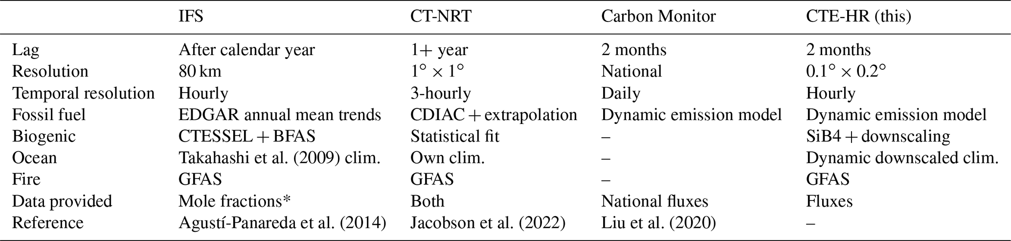
Here, we report on the development and evaluation of a high-resolution near-real-time CO₂ flux product covering Europe. We see the use of this flux product as twofold: (1) to rapidly gain insight into special events in the European carbon cycle such as the 2018 drought and (2) as an easily available starting point for atmospheric modeling or data assimilation of CO₂ over Europe. These foreseen applications also highlight where our product differs from existing emission products (such as fossil fuel emissions from CAMS, Kuenen et al., 2022, https://doi.org/10.24380/0vzb-a387, GridFED, Jones et al., 2021, and GRACED, Dou et al., 2021): we provide atmospheric modelers with an easy replacement for traditional bottom-up fluxes but with recent socioeconomic- and meteorology-informed dynamic fluxes at a high spatiotemporal resolution over Europe. Our product is freely available (CC-BY-4.0) with a lag time of about 2 months behind real time. As it also includes high-resolution fluxes from the biosphere, regridded fire emissions from the Global Fire Assimilation System (GFAS), and ocean (CarboScope-based) fluxes, it can be readily used in atmospheric modeling. Some other products that assess (parts of) the carbon cycle are shown in Table 1, which also clearly identifies the niche of our product. A third application, currently under development (but not yet completed), will merge the CTE-HR fluxes with the existing CarbonTracker Europe fluxes, with the aim of achieving the desired additional level of consistency with large-scale constraints.

Takahashi et al. (2009)Agustí-Panareda et al. (2014)Jacobson et al. (2022)Liu et al. (2020)

Table 1 Current CO₂ flux products. IFS: Integrated Forecast System (Agustí-Panareda et al., 2014); CT-NRT: CarbonTracker-Near Real-Time (Chen et al., 2019); EDGAR: Emission Database for Global Atmospheric Research (Janssens-Maenhout et al., 2019); CDIAC: Carbon Dioxide Information and Analysis Center (Andres et al., 1996); BFAS: Biosphere Flux Adjustment Scheme (Agustí-Panareda et al., 2016); clim.: climatology. * Only column-averaged CO₂. Prescribed fluxes are provided for completeness but should not be used like an analysis product (A. Anna Agustí-Panareda, personal communication, October 2021).

To document the fluxes and demonstrate their use, this paper is organized as follows: in Sect. 2 we explain how we created the different fluxes and which activity and meteorological data we use to create 0.2^∘ × 0.1^∘ hourly fluxes. We also describe our efforts to evaluate our fluxes using atmospheric transport modeling and analysis at district level for Amsterdam. In Sect. 3 we provide (a) the flux anomalies at large scales during the 2018 European drought and COVID-19 restrictions, (b) an assessment of mole fraction residuals on regional scales through transport modeling at Integrated Carbon Observation System (ICOS) sites, and (c) a local-scale comparison with fluxes measured in the city of Amsterdam. A discussion of the strengths, weaknesses, and implications of this work is given in Sect. 4, followed by the conclusion in Sect. 7.

2 Methods

2.1 High-resolution system

We create high resolution (0.2^∘ × 0.1^∘, hourly) for Europe (−15–35^∘ E, 33–72^∘ N) in near real time (2-month lag). To account for different parts of the European CO₂ budget, we combine multiple data streams. The different sources that we use to estimate fossil fuel, biogenic, oceanic and wildfire CO₂ fluxes are summarized in Fig. 1 and explained further in the following sections. The CTE-HR framework uses the CarbonTracker Data Assimilation Shell (CTDAS) framework to provide near-real-time flux estimates. These are not optimized with atmospheric data and can be used standalone, or they can later be optimized using CTE or other similar data assimilation systems.

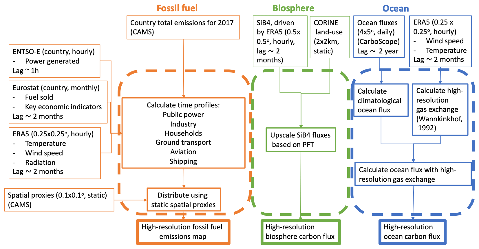
Figure 1 Flow chart of incoming data streams and their use in CTE-HR. The orange box shows the fossil fuel module, the blue box shows the data used for downscaling the ocean fluxes and the green box shows the calculation of the high-resolution biosphere fluxes. With all dynamic incoming data streams, the resolution and lag are shown. The individual products, such as CAMS, are described in the text.

2.1.1 Anthropogenic combustion emissions

Anthropogenic emissions are highly variable in time (e.g., Nassar et al., 2013; Mues et al., 2014) and are subject to socioeconomic factors as well as meteorology. Moreover, they are very heterogeneous in space; in this section, we elaborate on the spatiotemporal distribution of the anthropogenic combustion emissions using the Gridded Nomenclature For Reporting (GNFR) sector definitions, similarly to the CAMS dataset (Kuenen et al., 2022). The related data streams are highlighted in orange in Fig. 1.

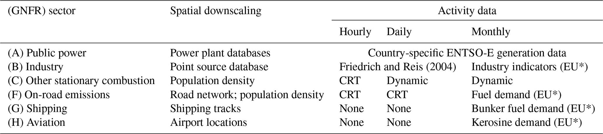
As a basis, we use the CO₂ emissions from 2017, as provided by country reports and compiled for the CAMS regional emission dataset (Kuenen et al., 2022). For all sectors except public power, these emissions are linked to activity data (e.g., amount of fuel sold). We then calculate the emission for the desired period by using activity data for that respective period (similarly to Super et al., 2020b). Note that, in this approach, we only scale activity data and not changes in the CO₂ emitted per activity. The used activity data are shown in Table 2. Public power data are taken from the European Network of Transmission System Operators for Electricity (ENTSO-E). Spatial distribution is done following Kuenen et al. (2022) and is summarized in Table 2 as well.

Friedrich and Reis (2004)

Table 2 Anthropogenic combustion sectors and their spatial and temporal downscaling proxies. “Dynamic” indicates a dependence on meteorology, whereas the CRT (CAMS-Regional Time profile) denotes static activity data taken from Guevara et al. (2021). “None” means a flat profile (i.e., no scaling based on activity) for that time period: if a sector has a flat monthly profile, every month is assumed to have the same emissions. EU*: Eurostat data. Note that we only include surface emissions.

Public power.

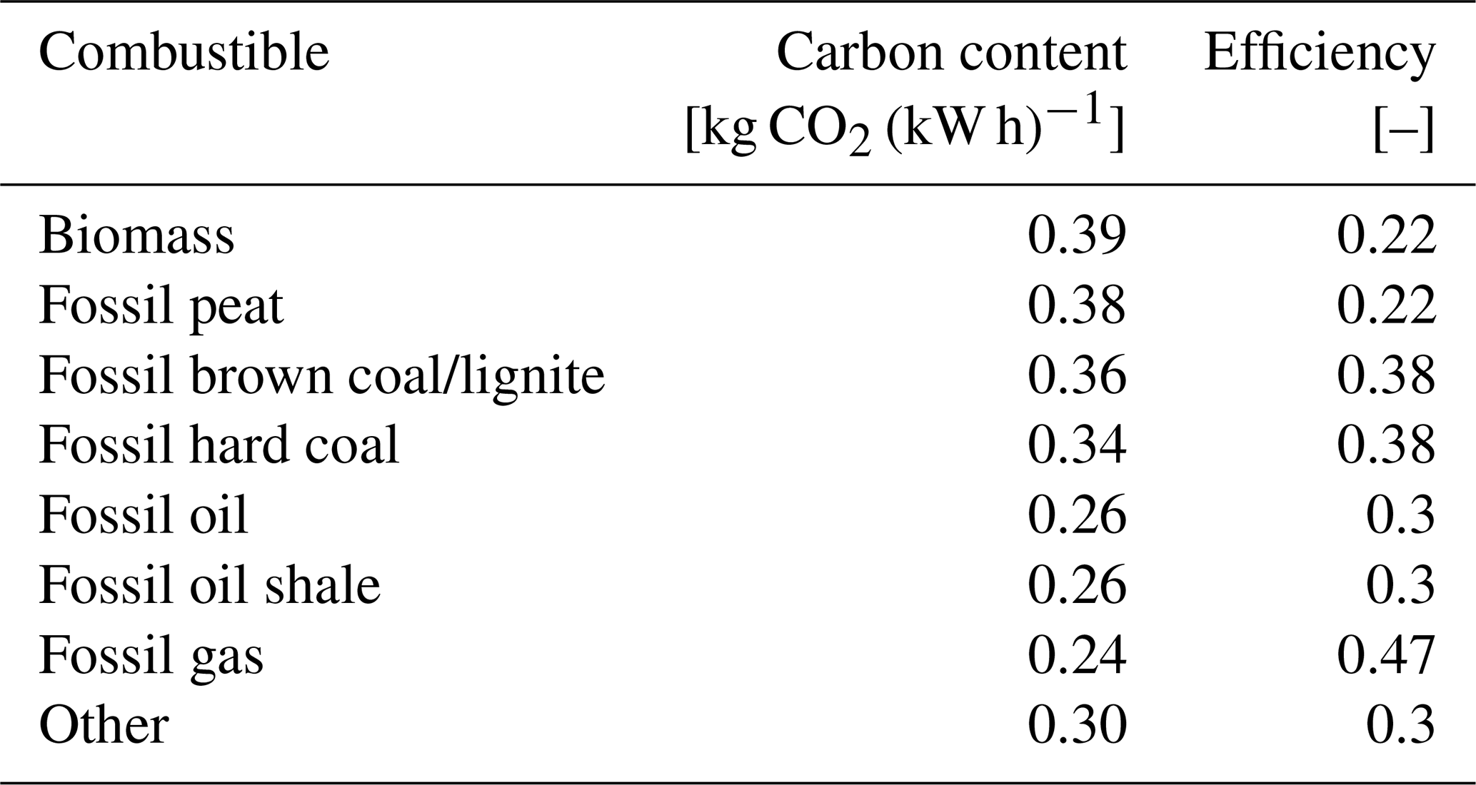
Emissions from the public power sector (GNFR sector A) are highly variable due to political actions (e.g., moving towards/from nuclear or the use of more biofuel), but social activities (e.g., Christmas Eve) and meteorological variability (e.g., air-conditioning use during heatwaves) determine energy use. We take hourly generation data by production type from ENTSO-E (https://transparency.entsoe.eu, last access: 27 January 2023). Generation by production type is translated into generation by fuel and then translated into CO₂ emissions, using $E=P\cdot C/\mathit{\eta }$, where E denotes the CO₂ emissions (kg), P is the energy produced (kWh), C is the carbon content of the fuel, and η is a fuel-specific efficiency. Values for C and η for different fuels are shown in Table 3. Note that we take biofuels into account here.

With the near-real-time ENTSO-E data, we capture variability in the CO₂ emissions of the public power sector due to variability in the amount of energy generated by renewable energy. This is shown in Sect. 2.2.2.

Table 3 Constants for electricity production from different fuels. Carbon contents are taken from Watter (2015), efficiencies from Hussy et al. (2014) and European Environment Agency (2016).

Not all countries in the European domain are included in the ENTSO-E database. Also, it can be that data are missing from the ENTSO-E database. These missing data are filled with Eurostat monthly data (https://ec.europa.eu/eurostat/databrowser/view/NRG_CB_PEM__custom_200961/, last access: 27 January 2023) and CAMS emissions, downscaled to hourly data if ENTSO-E data are not available for the respective country. This downscaling is achieved using the heating degree day (HDD) method and proxies for renewable energy, similarly to Super et al. (2020b). For this, we assume a temperature threshold of 25 ^∘C for coal-fired power plants (Super et al., 2020b). We also assume that the gas-fired power plants only show variability due to the variable generation of renewable energy and that oil- and biomass-fired power plants have static emissions, which is also seen in the ENTSO-E data. Power plants have a constant offset, representing generation for sources that use energy constantly. This constant offset depends on the country and month and is calculated from the available ENTSO-E and Eurostat data, respectively. If no data are available for a country, it is assumed that the offset for that country is the same as for the whole of Europe. The downscaled Eurostat data have a Pearson R of 0.5 to 0.9 compared to the ENTSO-E data, depending on the country and period tested. The country total CO₂ emissions, as calculated by the HDD method and Eurostat data, differ by a maximum of 10 % per week compared to the ENTSO-E data. The spatial distribution applied is the same as in Kuenen et al. (2022). Although different combustibles are included in CTE-HR, we do not differentiate between different generation units within the country; i.e., country-wide generation is projected onto the relative emissions from CAMS.

Industry.

Emissions from the industry sector (GNFR sector B) are sensitive to societal and economic changes. We calculate a monthly specific scaling factor relative to 2017 for industry production volume, provided by Eurostat. The production volume is, amongst others, based on turnover of capitalized production and changes in stocks (https://ec.europa.eu/eurostat/cache/metadata/en/sts_esms.htm, last access: 27 January 2023). We use season- and calendar-adjusted data.

If the industry production data are not (yet) available for the current month, it is assumed that, for that country and month, the relative production volume is equal to the average of Europe. If European data are not present, we use the previous available month for the respective country. Hourly emissions are calculated from these monthly emissions following Friedrich and Reis (2004), and the spatial distribution is from Kuenen et al. (2022).

Other stationary combustion.

GNFR sector C, other stationary combustion, includes household emissions but also the commercial and institutional sectors as well as other stationary sectors. Here, we assume that the stationary combustion CO₂ emissions depend mostly on outdoor temperature, as most CO₂ is emitted for heating. Therefore, we use the heating degree day (HDD) method (Mues et al., 2014; Super et al., 2020b). We use a temperature threshold for heating of 18 ^∘C and a constant offset (representing non-temperature-dependent emissions, such as cooking) of 0.1 for all countries, similarly to Mues et al. (2014) and Super et al. (2020b). For a more elaborate description of the HDD method, see Mues et al. (2014). The daily emissions calculated using the HDD method are downscaled to hourly emissions using static profiles by Guevara et al. (2021). The spatial distribution of the emissions is the same as in Kuenen et al. (2022).

On-road emissions.

The on-road sector, GNFR F, includes all on-road transport, i.e., passenger cars and light- and heavy-duty vehicles. We do not distinguish between different subsectors and therefore only account for the total CO₂ emissions on the road. The amount of traffic on the road is highly variable in time, and therefore traffic emissions are also highly variable. Monthly petrol demand from EuroStat, relative to 2017, is used to scale the emissions (https://ec.europa.eu/eurostat/databrowser/view/nrg_jodi/default/table?lang=en, last access: 27 January 2023). Additionally, gridded daily and hourly time factors are taken from Guevara et al. (2021). Note that these diurnal profiles are different for weekdays and weekend days but do not include socioeconomic changes such as the COVID-19 crisis. Therefore, the diurnal cycles during, e.g., the COVID-19 pandemic might differ, but this does not affect total (monthly) emissions. We apply the same spatial distribution as Kuenen et al. (2022).

Shipping.

Shipping emissions, GNFR sector G, depend highly on economic activity. We scale monthly shipping emissions with the demand of fuel oil from Eurostat relative to 2017 (https://ec.europa.eu/eurostat/databrowser/view/nrg_jodi/default/table?lang=en, last access: 27 January 2023). On a yearly basis, this correlates well with available CAMS emissions (not shown). The spatial distribution is assumed to be static and is taken from Kuenen et al. (2022).

Aviation.

Similarly to shipping emissions, we scale monthly aviation emissions (GNFR sector H) based on the demand of fuel (kerosine), as supplied by Eurostat (https://ec.europa.eu/eurostat/databrowser/view/nrg_jodi/default/table?lang=en, last access: 27 January 2023). Note that, as we use the GNFR sector definitions, only takeoff and landings are included (United Nations economic comission for Europe, 2014). We take the location of airports from Kuenen et al. (2022) and assume these locations to be static. Therefore, this does not account for newly built airports.

Off-road emissions.

Off-road emissions include tractors, construction machinery, trains, and other mobile emission sources that are off-road (GNFR sector I). Currently, the CAMS emissions from the last available year are used, assuming no temporal downscaling. The spatial distribution is taken from Kuenen et al. (2022).

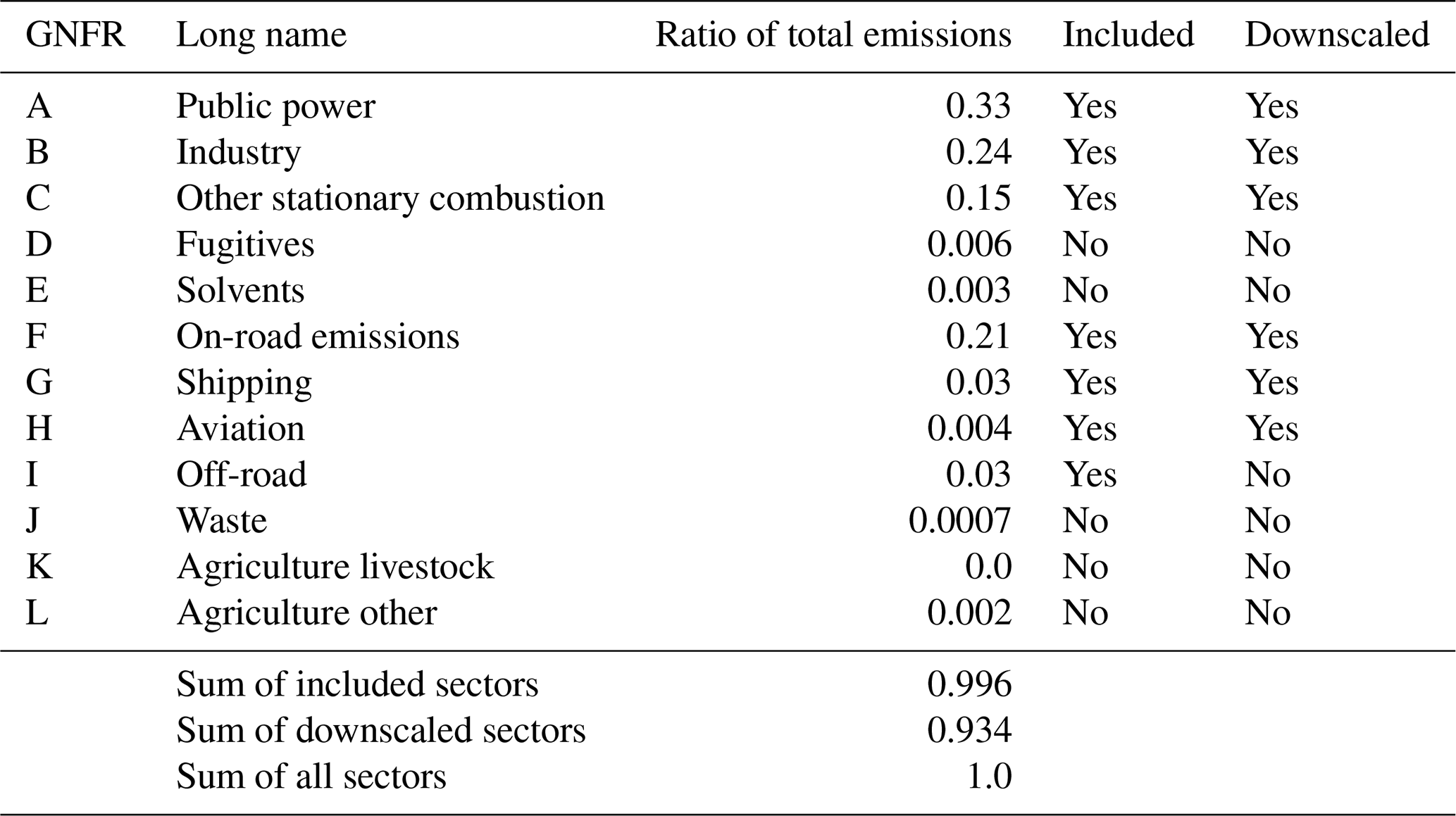
A summary of the relative contributions of all sectors included is shown in Table 4. The resulting CO₂ emissions from fossil fuels for 8 July 2018, 12:00 UTC as calculated by the model are shown in Fig. 2. Note that fluxes at this resolution can be created with a lag of about 2 months (see Fig. 1).

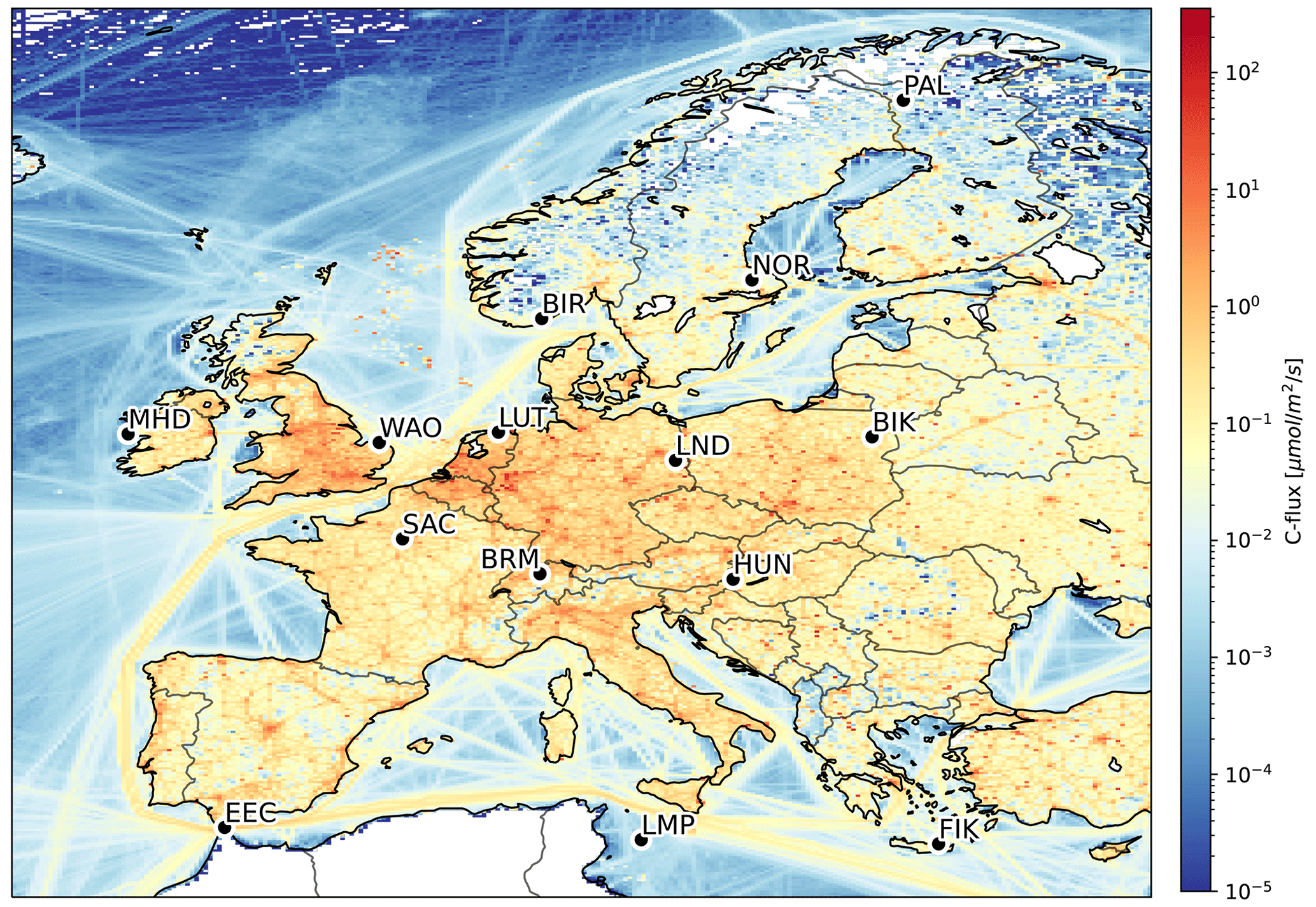
Figure 2 Estimated anthropogenic combustion emissions for 8 July 2018, 12:00 UTC as an example of the anthropogenic emission part of our product. Black dots indicate the location of used ICOS CO₂ measurement sites.

Table 4 Ratio of total CO₂ emissions from CAMS for 2017. The included column shows whether a sector is included in the final data product and included in the emissions presented in the remainder of this paper. Downscaled sectors are subject to near-real-time information as described in the text.

2.1.2 Emissions from cement production

For 2018, the calcination of cement accounts for about 8 % of the anthropogenic CO₂ emissions in the domain. We include these fluxes by taking GridFED calcination fluxes from the last available year, currently without near-real-time scaling. Note that, for the analysis, we use Version 2021.1, but the released fluxes will contain the newest version (Version 2021.3). The carbonation of cement is currently not included. This sink accounts for about 2 % of the total anthropogenic emissions (Friedlingstein et al., 2022b).

2.1.3 Biosphere fluxes

Hourly biosphere fluxes inside the high-resolution domain are calculated with the Simple Biosphere Version 4 (SiB4) (Haynes et al., 2019). SiB4 is driven by ECMWF Reanalysis 5th Generation (ERA5) meteorological input data (Hersbach et al., 2020) and restarted from a 5×20-year spinup. We use a constant atmospheric CO₂ mole fraction of 370 ppm, resulting in a neutral steady-state biosphere. Fires are not accounted for in the spinup. Before each simulation, a 3-year run with constant CO₂ is used as additional spinup to equilibrate croplands.

To better account for water stress, we increased the drought sensitivity of evergreen needleleaf forests and croplands by modifying the rooting depth of these two plant functional types (PFTs), similarly to Smith et al. (2020). Note that we do not scale precipitation from the ERA5 input using the global precipitation reanalysis product (GPCP), unlike Baker et al. (2010) did for SiB4 driven by the Modern-Era Retrospective analysis for Research and Applications Version 2 (MERRA2) meteorology, as the scaling resulted in nonphysical jumps in biosphere fluxes between GPCP (2.5×2.5^∘) grid cells. We used unscaled precipitation from ERA5, assuming it is a reliable precipitation product for Europe.

In SiB4, the net ecosystem production (NEP) is calculated from the gross primary production (GPP) and total ecosystem respiration (TER). GPP, TER, and NEP are calculated for the 10 most dominant PFTs in a grid cell. We map the calculated PFT-specific fluxes at 0.5 × 0.5^∘ to high resolution (up to 2 km) using the coordination of information on the environment (CORINE) land-use classification (Bossard et al., 2000). We translated the CORINE land-use classes into SiB4 PFTs as shown in Table 5.

Table 5 SiB4 PFT names and their corresponding CORINE land-use classes' grid codes. For the CORINE classification, see http://clc.gios.gov.pl/doc/clc/CLC_Legend_EN.pdf (last access: 27 January 2023).

The effect of the high-resolution land-use map is shown in Fig. 3. In the eastern part of the domain, no CORINE data are available and no downscaling is applied, resulting in relatively coarse spatial flux patterns. This is highlighted in the insets in Fig. 3c and d. See Appendix 2.2.1 for a further validation of this aspect.

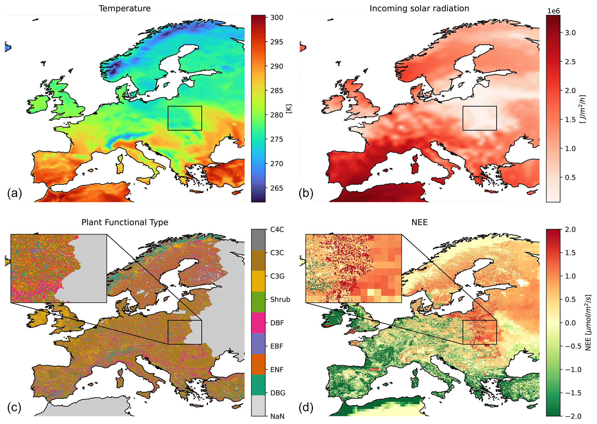
Figure 3 Temperature (a) and incoming solar radiation from ERA5 (b), high-resolution plant-functional type from the CORINE land-use classification and (c) NEE from CTE-HR over Europe (d) for 1 April 2018, 14:00 UTC. The inset shows a close-up on the border of where high-resolution land-use data are available to illustrate the difference.

2.1.4 Emissions from fires

Wildfire CO₂ emissions are taken from the GFAS (Di Giuseppe et al., 2018). The 0.1 × 0.1^∘ daily fluxes are binned to the 0.1 × 0.2^∘ domain for ease of use.

2.1.5 Ocean fluxes

Ocean CO₂ exchange responds to the difference in partial pressure (ΔP) of CO₂ in the water and atmosphere and temperature and wind speed (Wanninkhof, 1992). Assuming constant ΔP, we scale CarboScope climatological ocean fluxes of the 10 most recently available years (Rödenbeck et al., 2013) based on the gas-exchange coefficient k (Wanninkhof, 1992). The high-resolution flux is calculated as $F=F_{\mathrm{clim}}\cdot k/k_{\mathrm{clim}}$, where F is the ocean–atmosphere CO₂ flux and the subscript “clim” indicates a 10-year climatology over the last available years. Climatological ocean fluxes are created from the CarboScope product (Rödenbeck et al., 2013). k is calculated following Wanninkhof (1992):

$$\begin{array}{}\text{(1)}& k=\mathrm{0.31}\cdot u^{\mathrm{2}}/\sqrt{\mathit{Sc}/\mathrm{660}},\end{array}$$

where Sc is the Schmidt number, calculated by a third-order function of sea surface temperature (Wanninkhof, 1992), and u is the 10 m wind speed. As u and temperature are available at high resolution, ocean fluxes can be calculated at a high resolution as well. We note that more detailed European air–sea spatial flux patterns can be derived from ICOS observations of pCO₂ (Becker et al., 2021), and a recently developed machine-learned monthly flux product can be considered to underlie our hourly fluxes if regularly updated.

2.2 Validation of the downscaling

2.2.1 SiB4 downscaling

A validation of the downscaling of the CTE-HR SiB4 fluxes is shown in Fig. 4, where we show the spatial correlation coefficient between GPP fluxes in CTE-HR and MODIS-derived Near-Infrared Reflection of vegetation (NIRv; see Badgley et al., 2019), both at 0.05^∘ (where CTE-HR fluxes were regridded using nearest-neighbor resampling). The correlation is calculated over N=100 high-resolution pixels within each of the larger 0.5 × 0.5^∘ boxes for July 2016. A positive correlation coefficient between observed NIRv and simulated GPP suggests that credible sub-0.5^∘ gradients were present in the high-resolution CTE-HR fluxes, even though they were originally calculated at a coarser (0.5^∘) resolution in SiB4. We find that for 1795 (56 %) of the larger grid boxes, the spatial downscaling indeed represents the observed gradient in a statistically significant correlation. For 507 larger grid boxes (16 %), the observed spatial gradient is misrepresented, and for 894 boxes (28 %), no conclusions can be drawn due to a lack of observed variability or a lack of a significant correlation within the 0.5 × 0.5^∘ grid box. A similar result was found for other months in the growing season (when GPP is higher) and demonstrates that the downscaled biosphere fluxes are in the majority of boxes better than (54 %) or at least as good as (28 %) the SiB4 fluxes without downscaling.

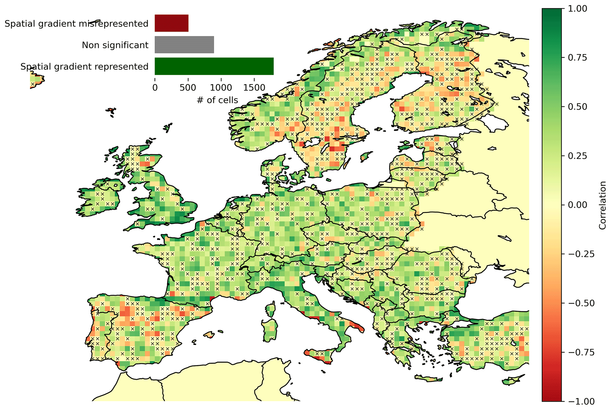
Figure 4 Correlation coefficient between NIRv and the downscaled SiB4 product from CTE-HR within 0.5×0.5^∘ grid cells for July 2016. Non-significant values are marked with a cross. The inset in the upper left shows the number of grid cells where the spatial gradient was represented or misrepresented or no significant correlation was found.

2.2.2 Added value of the ENTSO-E data

The added value of ENTSO-E power usage data – relative to monthly data as used widely in the community – mainly shows in specific cases where deviations from the mean flux are large. An example of this occurred during Christmas 2017 in Germany when, due to high wind speeds and an abundance of sustainable energy, German electricity prices became negative. This event was widely covered in the media (e.g., Berke, 2017). With the ENTSO-E data, our CTE-HR emissions capture this increase in wind-generated electricity and the corresponding decrease in energy generation by the combustion of fossil coal and gas. This is shown in Fig. A1 in Appendix A, demonstrating the added value over a lower temporal resolution view such as provided by the CAMS emission dataset. We emphasize that the differences between the public power flux according to CAMS-REG-GHG emissions and the ENTSO-E data are about one-third of the biosphere fluxes in Germany during December, and an error due to monthly constant anthropogenic emissions is thus unlikely to be corrected using atmospheric in situ or space-based data. Instead, the reduced emissions from power generation would be wrongly attributed to the biosphere fluxes or to other larger emission sources if no sub-monthly data on power generation were available in the underlying emissions.

2.3 Methodology for the comparison to atmospheric measurements

2.3.1 Poor person's inversion

We compare our high-resolution system (CTE-HR) to a poor person's inversion (PPI), similar to the poor man's inversion from Chevallier et al. (2009). The PPI is a relatively simple way of estimating the biosphere fluxes based on the global atmospheric growth rate of CO₂ and used as a benchmark here. In our PPI, global CO₂ fluxes from anthropogenic emissions, ecosystem respiration, ocean exchange and wildfires are summed and compared to the atmospheric growth rate of CO₂. Prior gross primary production is then scaled, so that the sum of the fluxes follows the global atmospheric growth rate:

$$\begin{array}{}\text{(2)}& \mathit{\alpha }\text{GPP}+\text{TER}+\text{FF}+\text{ocean}+\text{fire}=G,\end{array}$$

where GPP is the prior gross primary production, α is a scaling factor to close the budget, TER is the total ecosystem respiration, and FF is the anthropogenic CO₂ fluxes, including anthropogenic combustion emissions and cement production. “Ocean” is the oceanic CO₂ exchange, “fire” is the CO₂ emissions by wildfire, and G is the monthly atmospheric growth rate of CO₂. We chose to scale GPP in the PPI, as directly scaling NEE resulted in nonphysical fluxes (e.g., flipped diurnal cycles). Compared to TER, GPP has a larger interannual variability (Piao et al., 2020), and we therefore expected GPP to be a larger contributor to changes in the atmospheric carbon content than TER. We calculate TER and the prior GPP from a 10-year climatology of SiB4 (Haynes et al., 2019). This climatology was calculated over the 10 most recent years (2007–2017) based on a run that uses a spinup iterated five times over 2000 to 2020. To get a correct representation of the carbon pools, we include fires in this spinup. A diurnal cycle of GPP and TER is imposed based on a SiB4 simulation with a constant atmospheric CO₂ of 370 ppm and no fires. The 3-hourly output was interpolated linearly to hourly values. The atmospheric growth rate G is calculated from the NOAA global growth rate (https://gml.noaa.gov/ccgg/trends/gl_data.html, last access: 27 January 2023) and a conversion factor of 2.086 GtC ppm⁻¹, similarly to Chevallier et al. (2019). Anthropogenic CO₂ emissions are taken from GridFED from the previous year (Jones et al., 2021) and binned to a 1×1^∘ grid. We do not extrapolate the anthropogenic CO₂ emissions, as these changes in emissions are generally quite small (within a few percent) and unknown in near real time. Daily ocean emissions are taken from a climatology of the 10 most recent years from the CarboScope ocean inversion and bilinearly interpolated to 1×1^∘ (Rödenbeck et al., 2013). Fire emissions for the current month are taken from GFAS (Di Giuseppe et al., 2018) and binned to a 1×1^∘ grid.

Note that our approach differs slightly from Chevallier et al. (2009), as they scale NEE based on the uncertainty in their biosphere model. For this, they use a static, manually fitted scaling factor, whereas we exactly follow the monthly growth rate.

2.3.2 Large-scale atmospheric transport

To compare the fluxes from CTE-HR to the PPI, we assess mole fraction residuals at the continental scale. Hitherto, we propagated the different fluxes (Sect. 2.1–2.3.1) using the TM5 atmospheric transport model (Krol et al., 2005). We sampled CO₂ mole fractions at European ICOS sites (Ramonet et al., 2020; Drought 2018 Team and ICOS Atmosphere Thematic Centre, 2020). Similarly to Smith et al. (2020), we use a global resolution of 3^∘ × 2^∘ and nested zoom regions of 1×1^∘ over North America and Europe. Atmospheric transport is driven by meteorological fields from ERA5 (Hersbach et al., 2020). Although the 1^∘ resolution is coarser than the high-resolution fluxes, we here mostly show temporal variability in the CO₂ fluxes and mole fractions. Moreover, ICOS sites are generally located far away from large urban areas, allowing very local (FF) sources to mix through the atmosphere before they arrive at a measurement site, making high-resolution atmospheric transport less important. To get an overall idea of the performance of CTE-HR, we selected one site from each available country. In this selection, we made sure that the selected sites cover a range of latitudes, longitudes and flux landscapes. The selected sites are shown in Fig. 2. For these sites, we evaluate the root mean square error (RMSE) and correlation coefficient (R) between the simulated and observed CO₂ mole fractions. For the analysis with TM5, we discarded the 2.5 % days with the highest and lowest RMSEs to remove events that are not captured by the transport model.

As our product is not informed by large-scale constraints, we do not expect it to perform well over multi-annual timescales. However, as it contains much information on temporal variability, we do expect it to perform well on shorter, synoptic timescales. Therefore, we restart TM5 every month of 2018 from an initial CO₂ field taken from the CarbonTracker Europe (CTE2021) contribution to the GCP2021 release (Van der Laan-Luijkx et al., 2017; Friedlingstein et al., 2022a) and transport the fluxes for 5 weeks. Outside the high-resolution domain, we use PPI fluxes for atmospheric transport by TM5.

2.3.3 High-resolution transport

To test higher-resolution transport, we analyzed simulated and measured hourly mole fractions at the Lutjewad station in the Netherlands (53.24^∘ N, 6.21^∘ E) (LUT in Fig. 2). In Lutjewad, fossil fuel emissions, biosphere exchange, and advection of background air (from the North Sea) shape the measured CO₂ record (Bozhinova et al., 2014; Van der Laan et al., 2010).

The mole fractions are the result of transport by the Lagrangian particle model STILT (Lin et al., 2003) at 0.1 × 0.2^∘ resolution. The STILT model was driven by 3-hourly meteorological fields from the ECMWF-IFS short-term forecasts (following the IFS cycle development; for more information, see https://www.ecmwf.int/en/publications/ifs-documentation (last access: 27 January 2023). We released 100 particles and followed them for 10 d back in the atmosphere. We estimated the background CO₂ signal, taking into account the average location of the 100 particles at the end of the 10 d back trajectory. The STILT domain covered the same spatial extent as the CTE-HR domain. Background mole fractions were taken from CTE2021. We compare the high-resolution product CTE-HR to a 1×1^∘ version of CTE-HR (coarse) and the CTE-HR product without any temporal variability (flat, i.e., the temporal average of the 10 previous days). For each hourly time interval, we selected the cases where the difference in mole fraction between the three versions of the CTE-HR model is larger than 2 ppm. These cases indicate relatively large differences between transport of the full-resolution fluxes and those with a lower spatial resolution or a flat temporal profile. To analyze the influence of high-resolution transport on the capability to resolve different sectors, we transported each fossil fuel sector individually.

2.3.4 Local fluxes

To assess the performance of our model on a local scale, we compare the CTE-HR fluxes in Amsterdam to an eddy covariance tower in the center of the city. The tower is located at 52.366548^∘ N, 4.893020^∘ E at about 40 m above ground level, about 20 m above the average building height (Steeneveld et al., 2020). Note that the footprint of this tower (about 500 m) is much smaller than a grid box in CTE-HR (about 15 km). To be more representative of Amsterdam, we average the four grid boxes around the eddy covariance tower.

3 Results

We performed several tests to assess the performance and limitations of our modeled fluxes. First of all, we assess the skill of CTE-HR in dealing with anomalous events in the biosphere and for fossil fuel emissions. Secondly, we assess how well our fluxes can be used to represent the measured CO₂ mole fractions in the atmosphere over the entire European continent. We also performed a similar test on a much smaller scale with a higher-resolution transport model to assess the benefits of the high spatial and temporal resolution of the CTE-HR fluxes. Finally, we compare CTE-HR fluxes with those of eddy covariance CO₂ flux measurements in the city of Amsterdam to assess the representativeness of the diurnal cycle of our fossil fuel emissions in urban areas.

3.1 Continental and monthly scales: anomalies over Europe

Our fluxes are designed to be versatile enough to represent the biosphere and fossil fuel emissions in both normal and anomalous years. We illustrate this capability using two cases: the biosphere response to the 2018 European drought and the changes in fossil fuel emissions due to the 2020 COVID-19 restrictions.

Our CTE-HR biosphere flux anomalies during the 2018 European drought follow those of CTE presented by Smith et al. (2020), which were the result of inverse modeling of atmospheric CO₂ mole fractions (Fig. 5). Similarly to Smith et al. (2020), the CTE-HR fluxes show enhanced spring uptake in 2018 over Europe compared to 2016–2017 as well as reduced uptake during the summer drought (see Fig. 5a and b, respectively). This progression is also shown in panel (c), showing the total biosphere anomaly in the area influenced by the drought, as defined by Smith et al. (2020). Although both patterns in Fig. 5c are similar, differences over the affected area of roughly 20 TgC / month are present for May–August. This shows that both the spring uptake and the drought response are underestimated in the SiB4 fluxes, which is very similar to the model setup used for the prior estimate in Smith et al. (2020) (not shown). Atmospheric measurements hence added significant value to the prior SiB4 model in this case. Nevertheless, the similarity between the flux products indicates that we already capture anomalous periods in the biosphere reasonably well, without the need for computationally and time-consuming inverse modeling and delays due to data availability. CTE-HR therefore allows early recognition of such anomalies and possibly more rapid analyses of available atmospheric observations such as those collected by ICOS.

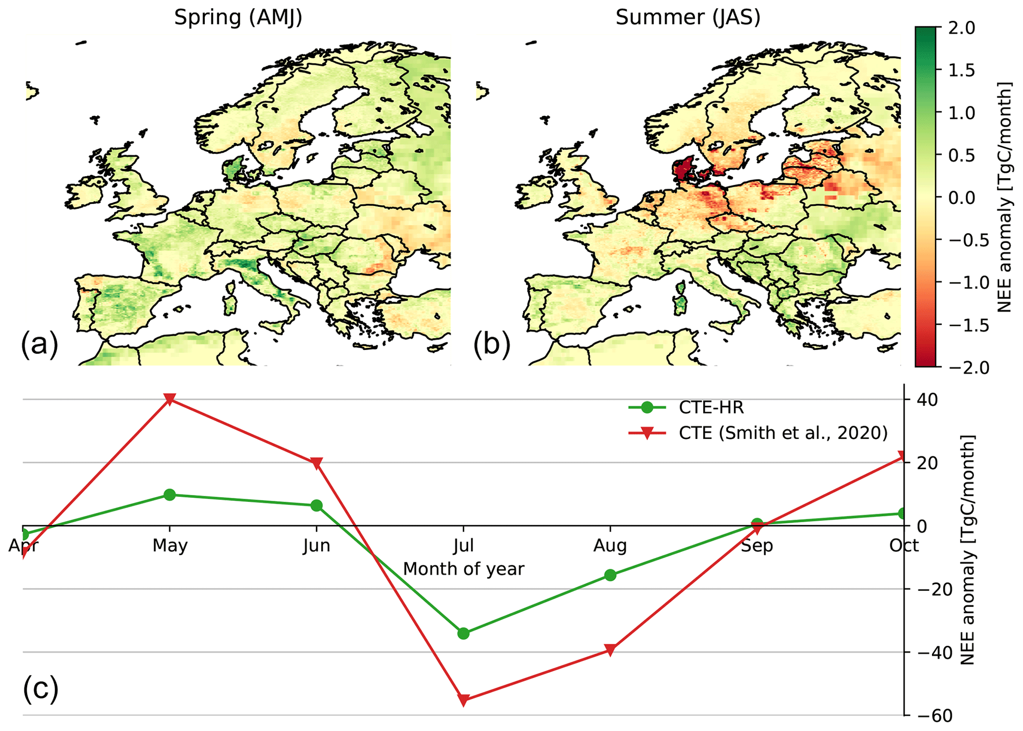
Figure 5 Estimated biosphere flux anomalies in 2018 compared to 2016–2017 for the spring (a) and summer (b) and the progression of the drought under the area influenced by the drought according to Smith et al. (2020) (c). Anomalies following Smith et al. (2020) are also shown for comparison. Note that Smith et al. (2020) show their anomalies relative to 2013–2017.

Global anthropogenic combustion emissions in 2020 decreased due to the global COVID-19 pandemic (Guevara et al., 2022; Le Quéré et al., 2020; Dou et al., 2021), something also visible in our European fossil fluxes (Fig. 6). In CTE-HR, total European emissions decreased by 7 % in 2020 compared to 2019, which is consistent with the values reported by https://carbonmonitor.org (last access: 27 January 2023) (Liu et al., 2020) (who report a decrease of 7.5 %, not accounting for international aviation) and Guevara et al. (2022) (who report decreases of 7.8 % and 3.3 % for fossil fuel and biofuel CO₂ emissions, respectively). Figure 6 shows that the decrease is highly sector-specific (lower panel), with the aviation sector showing the highest percent decrease (80 %) during lockdowns (indicated in grey shading) compared to 2019. Also, on-road, industry, and shipping emissions decreased (30 %, 30 %, and 20 % maxima, respectively). As the on-road and industry sectors contributed more to the total CO₂ emissions in the domain (see Fig. 6, upper panel), their decrease impacts the total reduction more than the aviation sector. The found reductions are similar to Le Quéré et al. (2020) and https://carbonmonitor.org, who show decreases of roughly 80 % in the aviation sector and 30 % for the industry sector during lockdowns. Note that the emissions from the industry sector are estimated by Le Quéré et al. (2020) based on plants in the USA and China. In contrast to Le Quéré et al. (2020), we do not find an increase in household heating emissions due to the COVID-19 confinement, but we note that in CTE-HR, household emissions only respond to temperature and not to socioeconomic changes. Overall, though, the results presented here show that the fossil fuel emissions from CTE-HR respond to socioeconomic changes in a realistic way and hence capture much of the expected emission variability over timescales of weeks or months.

Figure 6 The relative sector share to total emissions in 2020 for 2-month periods is shown in the pie charts. Relative emissions compared to 2019 per sector calculated by a 28 d rolling average are shown in the line graph. The grey shading indicates periods with lockdowns, and the number of European countries (out of 30) in lockdown as given by ECDC (2021) is indicated by the number in the grey bar. Household emissions are not included in the lower panel, as household emissions only respond to temperature here. Note that aviation has a relatively small share, as we only include emissions during landing and takeoff, following GNFR sector definitions.

3.2 Continental and monthly scales: mole fractions

CTE-HR is designed to be a good first-guess flux estimate for atmospheric modeling/data assimilation of CO₂. Hence, it will have added value if the transported fluxes result in simulated CO₂ mole fractions that are at least as close to the measurements as other methods that can be applied on a similarly short timescale. To test this, we compare our simulated mole fractions to a PPI (see Sect. 2.3.1) and mole fractions from the CTE2021 contribution to the Global Carbon Project (Van der Laan-Luijkx et al., 2017; Friedlingstein et al., 2022a), as simulated by TM5 across a selection of European ICOS sites (see Fig. 2).

On average, our transported fluxes result in better mole fractions (median RMSE = 3.96) at European ICOS sites compared to the PPI (median RMSE = 4.32), rivalling those of the CTE2021-optimized fluxes (RMSE = 3.95). This is indicated by the RMSE at the selected ICOS stations indicated in Fig. 7. For most stations we find a slightly higher RMSE compared to the inverse results of CTE2021 for the CTE-HR fluxes but a lower RMSE than for PPI. This difference becomes more pronounced near high-emission regions, where CTE-HR sometimes outperforms CTE2021 (e.g., at LUT, BIR, and BRM). Summarizing this across all sites confirms this good performance in mole fractions across Europe, and we confirmed that these results are not sensitive to the choice of stations by also assessing the performance for selections of the other stations. Corresponding to the lower RMSE, CTE-HR shows slightly higher correlations than CTE2021, as summarized for all stations in Europe (N=46; see Drought 2018 Team and ICOS Atmosphere Thematic Centre (2020), with the exception of Zeppelin and Station Nord, which fall outside our domain) in Table 6. This suggests that additional temporal variability is resolved with the high spatiotemporal resolution of the underlying fluxes. Overall, the CTE-HR product scores better than the PPI, which confirms that the dynamical modeling through proxies, such as temperature, and subcontinental gradients added through SiB4 represent true flux variations which would not be captured by simply projecting a global CO₂ growth rate onto a climatological GPP map for Europe.

Table 6 Fraction of the station months over all stations (N=46) for 2018 with a better statistical score than the threshold given in the header. The days with the highest and lowest 2.5 % RMSE are discarded to remove events that are not captured by TM5, resulting in different numbers of site months for the different runs.

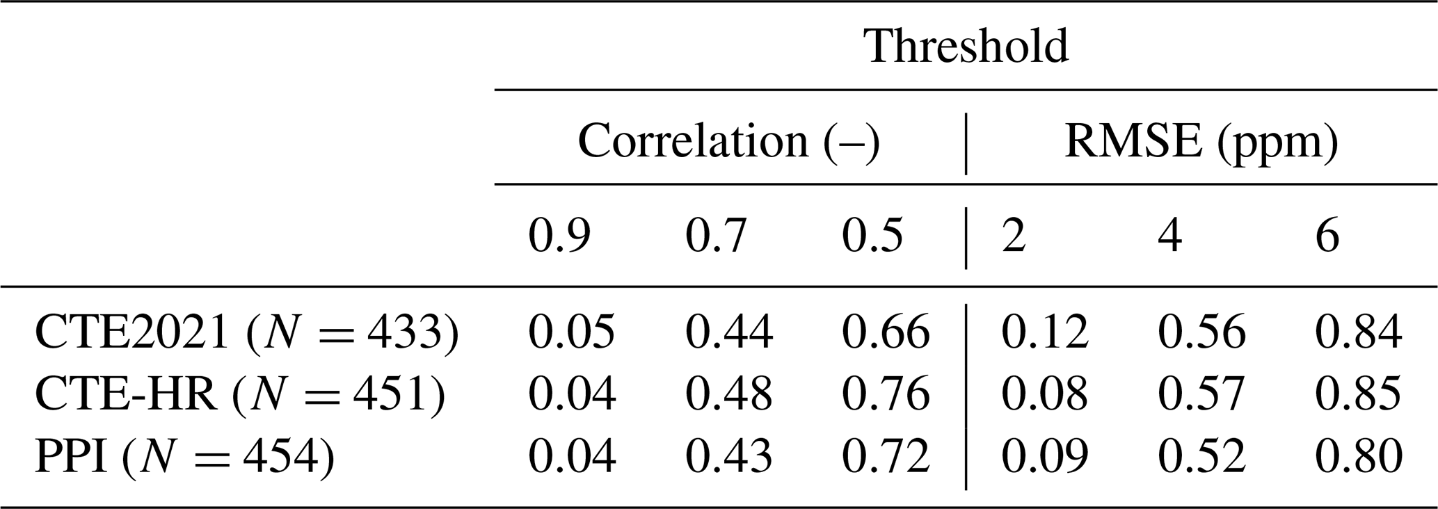
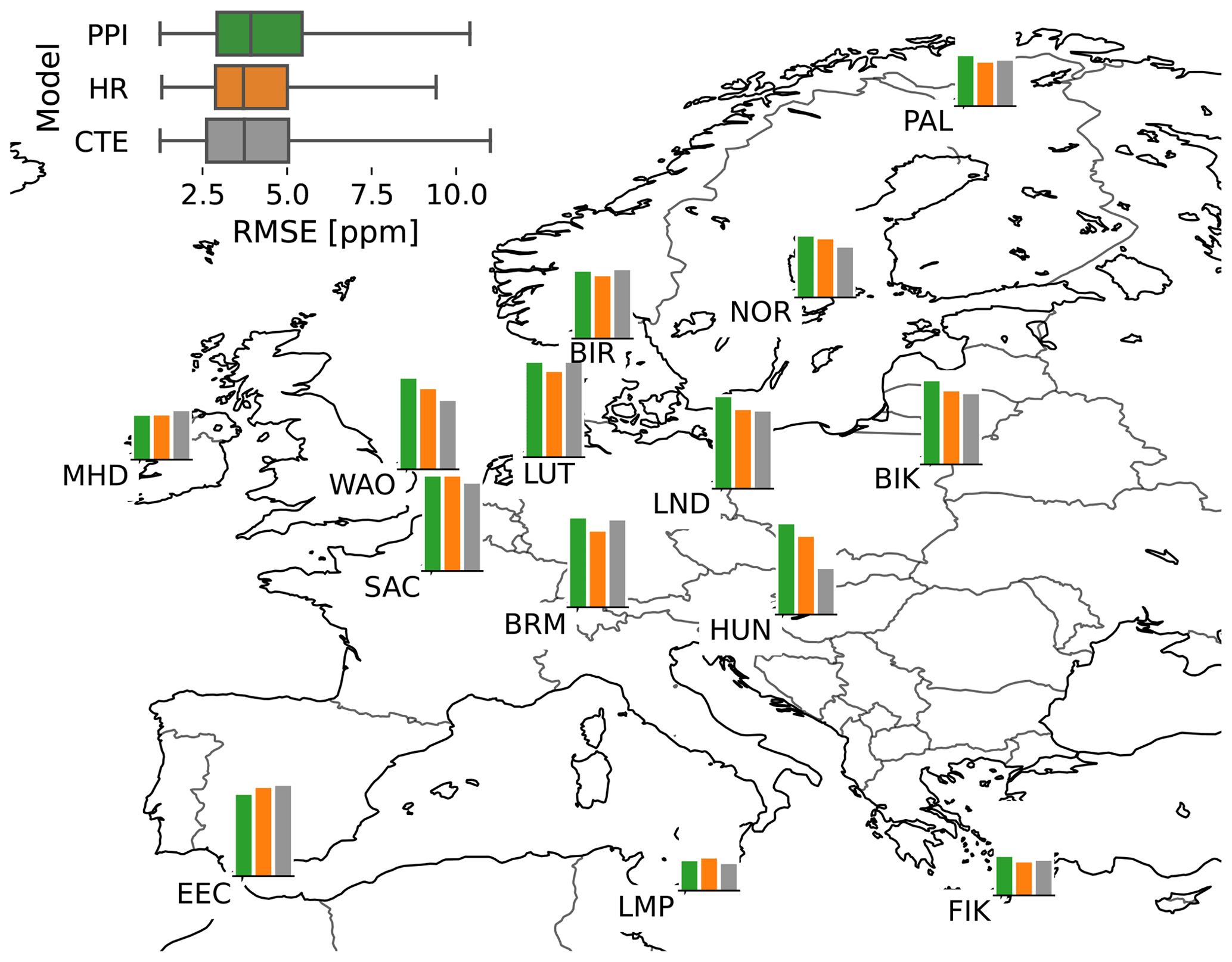
Figure 7 Root mean square error (RMSE) at selected stations in Europe. In the top left, a box plot of the monthly RMSE values is shown. PPI is the poor person's inversion, HR is the CTE-HR flux (this work) and CTE2021 is the latest CarbonTracker Europe release. Note that all the bars have the same y axis, which has a maximum of 6 ppm.

3.3 Regional and daily scales: Lutjewad

CTE-HR outperforms the PPI at the European continental scale, but it is also designed for use in regional- or country-scale analyses. To assess the performance of our fluxes at such scales, we analyze high-resolution transport at the regional scale for a selected site.

The time series of observed CO₂ mole fractions at the Lutjewad tower (Fig. 8) are generally well reproduced by the CTE-HR flux estimates when transported by STILT during well-mixed conditions (here assumed to be between 12:00 and 16:00 local time). During stable nighttime conditions, CTE-HR underestimates the CO₂ mole fractions (see Fig. 8b and c), which is a common problem in atmospheric transport modeling (Geels et al., 2007). Nighttime and early-morning observations most strongly reflect this, especially in winter months, when fossil fuel plumes, along with respired CO₂ from surrounding agricultural fields, contribute significantly to the observed peaks in the CO₂ signal. In the night (22:00–04:00 local time), the RMSE between the observed and simulated mole fractions is about 10 ppm, whereas under well-mixed conditions (10:00–16:00 local time), the RMSE is about 6 ppm.

When we compare the transported fluxes of the CTE-HR product with a coarse (1×1^∘, low resolution) or temporally flat version of CTE-HR fluxes, we generally see only small differences (Fig. 8a). Most notably, the largest differences between the high-resolution and temporally flat fluxes are when the biosphere is very active. In 64 % of the simulated hours in May, this difference is larger than 2 ppm. This generally occurs during the night, when the boundary layer is shallow and respiration dominates (see Fig. 8b). Of this 64 %, 99.2 % is dominated by differences in the prescribed biosphere fluxes. In contrast, the largest differences between the high-resolution and spatially coarsened fluxes are in December (see Fig. 8c), when the anthropogenic emissions are higher and biosphere fluxes smaller. For 28 % of the hours in December, the difference between the coarsened and high-resolution fluxes is larger than 2 ppm. Of these cases, 80 % are dominated by differences in the prescribed public power (GNFR A) fluxes. Note that the difference between the flattened and high-resolution fluxes in December is larger than 2 ppm in only 3.6 % of the hours.

Overall, our transported high-resolution fluxes result in good model performance for CO₂ at the Lutjewad tower. Differences between the high-resolution and spatially coarsened (1×1^∘) fluxes are mainly seen in the 10 %–20 % of the record when fossil fuel emissions are the dominant source of CO₂. Within the FF emissions, the largest differences are due to the public power sector, which has very local sources (power plants). The dominance of FF emissions here is not unexpected, as fossil fuel emissions vary by orders of magnitude at regional spatial scales. Therefore, the main advantage we found for CTE-HR fluxes is that higher spatial resolution enables better resolution of emission plumes from point sources. We found similar advantages and similar percentages for high spatial resolution fluxes at the nearby Cabauw tower (not shown), where point sources such as from power plants affect the measured CO₂ in a few percent of the hourly data.

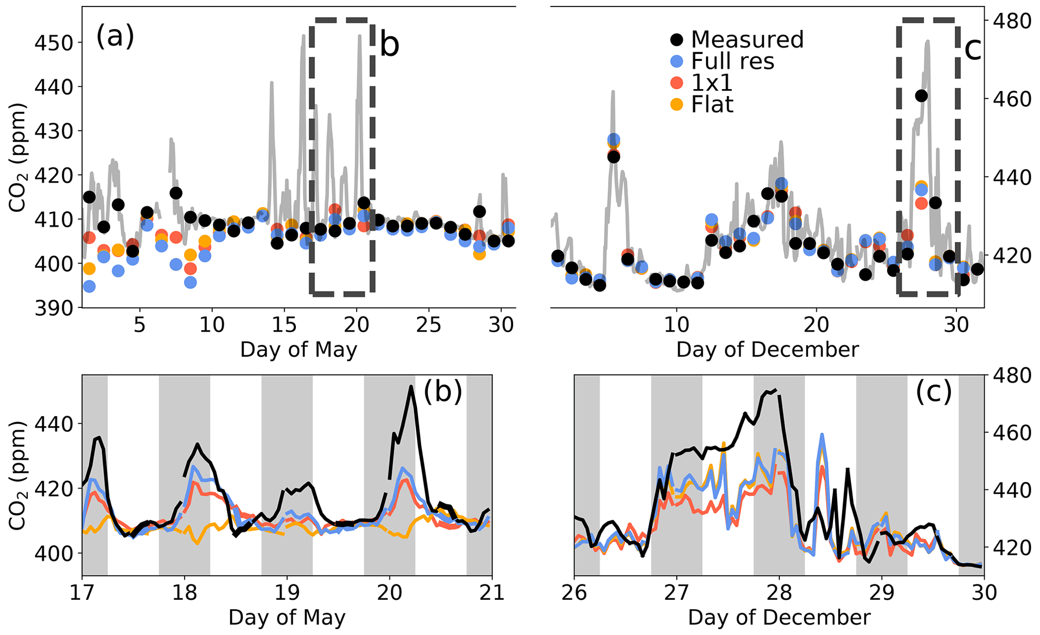
Figure 8 (a) Measured CO₂ time series at Lutjewad in the north of the Netherlands (53.24^∘ N, 6.21^∘ E) (grey lines), with a daily mean during well-mixed conditions (12:00–16:00 local time) indicated by black dots. Colored dots indicate afternoon mean (12:00–16:00 local time) modeled mole fractions for STILT transport of our flux product at full resolution (blue), transport using a 1×1^∘ coarsened version of our fluxes (red), and a version of our fluxes with flat diurnal cycles (orange). Panels (b) and (c) show zooms of (a) for May and December, respectively, with the full modeled time series. The periods between 18:00 and 06:00 are marked in grey to indicate the nights.

3.4 Local scale: Amsterdam urban fluxes

Eddy covariance measurements in Amsterdam as shown in Steeneveld et al. (2020) allow us to evaluate some aspects of our CTE-HR fossil fuel emissions in urban areas. Especially the short-term variability in the urban fluxes can be tested, since the measurements more directly relate to the actual urban fluxes and are not the result of an integrated signal over time as the CO₂ mole fractions.

Both the measured and modeled fluxes show a distinct diurnal cycle (Fig. 9), with maximum fluxes during the daytime and strong increases in flux in the morning. In summer, the peak of emissions is at midday, whereas in winter the peak of emissions occurs later in the day, which is reasonably well captured by CTE-HR. The magnitude of the estimated fluxes is lower than those in the eddy covariance measurements, especially in winter. However, since the footprint of the eddy covariance measurements covers a much smaller area (∼500 m) than our 0.1×0.2^∘ grid cells (Steeneveld et al., 2020), the magnitude of the fluxes will also be affected by a difference in land cover within the footprint. For instance, some of the averaged grid cells of the CTE-HR emissions are covered in water, and an industrial area is located in one of the four grid cells. This makes direct comparison of the magnitudes of the CTE-HR fluxes to the observations difficult. Despite these limitations of the comparison, it is clear that our diurnal and seasonal cycles add significant information compared to a flat profile (Fig. 9).

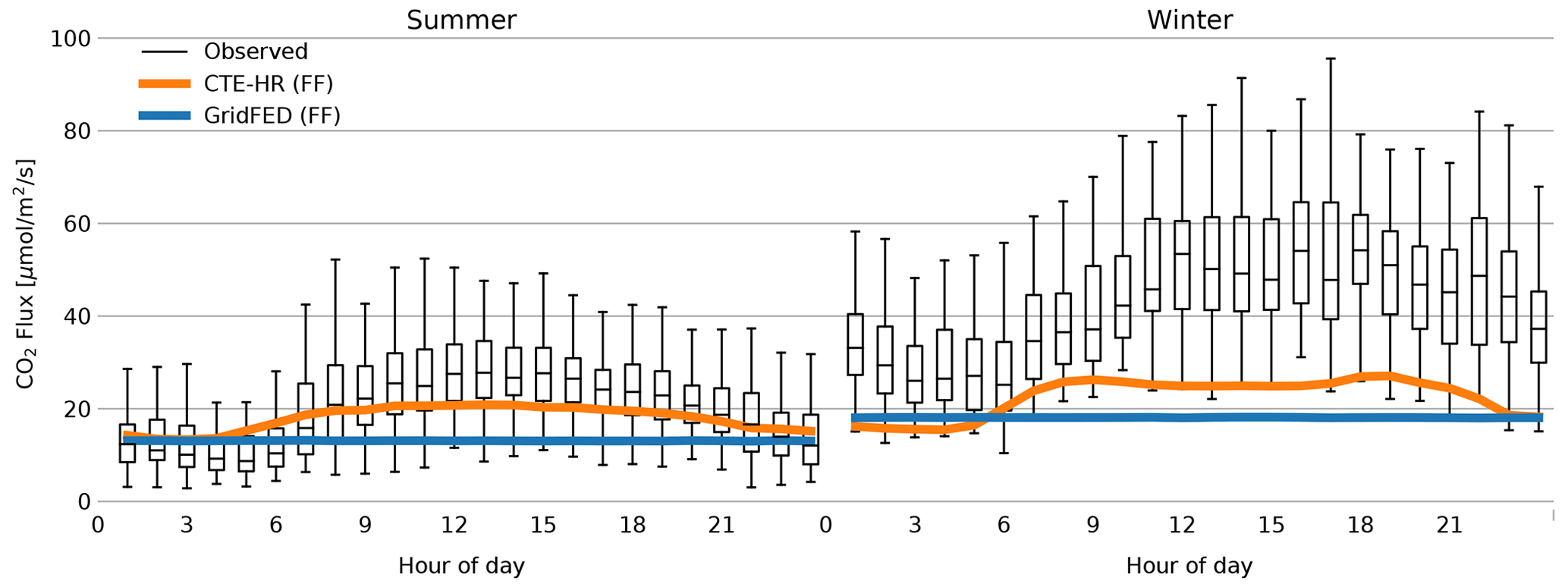
Figure 9 Average fluxes per hour of the day for the summer (MJJA) and winter (ND) of 2018 over Amsterdam. The box plots show the observed fluxes. Orange shows the Amsterdam emissions as calculated by our CTE-HR model, averaged over four grid boxes over Amsterdam (52.3^∘ N, 4.6^∘ E to 52.5^∘ N, 4.8^∘ E). The blue line shows the GridFED emissions (Jones et al., 2021), averaged over the same area as the CTE-HR emissions. September and October are not included in this figure, as there are large gaps in the observations in these months. Also, the first months of the year are missing, as the measurements started in May 2018.

4 Discussion

We present our high-resolution CO₂ CTE-HR flux product that provides European-scale carbon fluxes 2 months after real time with a 0.1^∘ × 0.2^∘ horizontal resolution. Below, we will discuss the anthropogenic and biosphere flux models, the atmospheric transport and a future outlook for CTE-HR. We end the discussion with our envisioned use of CTE-HR.

4.1 Anthropogenic emissions

On the Europe-wide annual scale, we find that our derived fossil fuel emission estimates agree well with state-of-the-art products such as GridFED (Version 2021.3) (Jones et al., 2021) showing a similar trend (not shown). Note however that GridFED provides only FF CO₂, whereas CTE-HR also includes biofuel emissions.

For the COVID-19 period in early 2020, we find a decrease in CO₂ emissions from industry, aviation, and ground transport and residential heating. These reductions mostly correspond to the findings of Liu et al. (2020) and Le Quéré et al. (2020), although the latter did not find reductions in the residential sector. We attribute this discrepancy to a difference in approach and study area, as Le Quéré et al. (2020) derived emissions for this sector from smart meters in the UK. Our approach, based only on temperature, results in reduced residential heating over Europe due to the warm winter, which was also shown by Liu et al. (2020). Both approaches are complementary, and in principle the smart meter approach is expected to give more accurate estimates, but these are not available Europe-wide or for all socioeconomic classes. On the other hand, our approach, based on temperature, is available for all residential areas. For energy production, both Liu et al. (2020) and Le Quéré et al. (2020) found a median decrease in CO₂ emissions from public power of roughly 10 % in 2020 compared to 2019, which is similar to the median decrease of 11 % that we find with CTE-HR. We do not find the regional increases in emissions over Europe for parts of France, Spain, Italy, and Germany that Dou et al. (2021) obtained. We attribute these differences to differences and changes in the spatial distribution of anthropogenic activity during the COVID-19 crisis. Dou et al. (2021) use satellite proxies to adjust regional estimates of emissions, whereas we use the most recent emission inventory data (Kuenen et al., 2022), which do not necessarily capture recent changes in the spatial distribution of emissions. The importance of such changes becomes evident during global crises, such as the COVID-19 pandemic, but can also be due to political and societal choices, such as expected decisions to move away from gas use across Europe. Other spatial discrepancies are introduced by the public power sector, which is the main fossil fuel sector. We use ENTSO-E data to resolve the temporal variability in this sector. However, we do not distinguish between different types of power plants (with the exception of nuclear), such as gas or coal spatially. We currently do not use this in our CTE-HR system, as detailed information about the spatial distributions of anthropogenic emissions (such as population density and industrial area) becomes available after roughly 2 years (Kuenen et al., 2022). Note that these outdated spatial distributions contribute significantly to the total uncertainty on grid-cell level.

Other major sources of uncertainty in the anthropogenic emissions from CTE-HR stem from (1) the use of proxies, such as Eurostat economic indicators for the CO₂ emissions from the industry, (2) the carbon intensities of fuels, to translate energy generated to CO₂ emissions from public power, and (3) temporal downscaling of yearly to hourly fluxes. An exact uncertainty estimate of the combined uncertainty in these sources is nearly impossible, as one has to account for all spatiotemporal correlations in the uncertainty structure. Our best estimate of the uncertainty in our anthropogenic fluxes is based on a similar approach by Super et al. (2020a) and Liu et al. (2020). Liu et al. (2020) found a daily, country total uncertainty of 7 % using a similar methodology. Super et al. (2020a) suggested that the scaling of country total emissions (uncertainty of ±2 %) down to the grid-cell level (1×1 km) increased the yearly uncertainty to 18 % of the flux, assuming a Gaussian error distribution. If we assume the spatial scaling error to our 15×15 km grid to also be 18 % (a possibly somewhat high estimate), and for this error to be independent of the temporal scaling error of 7 %, the addition in quadrature of these errors yields a total daily grid-cell uncertainty of 19.3 % of the calculated anthropogenic CO₂ flux. Due to a lack of knowledge about the correlation structure in these uncertainties, this is currently the best uncertainty estimate we can provide for the anthropogenic fluxes. Note however that some sectors (e.g., public power) have smaller uncertainties associated with them and that, therefore, generally, grid cells with larger fluxes have smaller uncertainties (Super et al., 2020a). The weight factors used in CTE-HR that represent diurnal and seasonal profiles of the anthropogenic CO₂ emissions do not include uncertainty estimates (Guevara et al., 2021), and therefore we cannot provide an exact uncertainty estimate for the hourly fluxes. From Super et al. (2020a), we estimate an added uncertainty of 2 % in country total CO₂ fluxes due to the temporal downscaling, looking only at well-mixed conditions.

4.2 Biosphere fluxes

4.2.1 Spatial downscaling

For CTE-HR, we applied further downscaling of our SiB4 fluxes using the CORINE land-use classes. The downscaling to 0.1^∘ × 0.2^∘ using CORINE is based on the assumption that, at the original resolution of SiB4 of 0.5^∘, differences in land use are more important for biosphere carbon exchange than meteorological variability, which we deem true for the synoptic timescale (see also Fig. 3). However, the downscaling also depends on the translation from land-use class to plant functional type, which is not straightforward for all land-use classes. An example of this is the land-use class “arable land”, which we translated to C₃ general plants. Nevertheless, resulting differences between the original SiB4 and the high-resolution biosphere fluxes are small (<5 % difference in total monthly flux for 2017–2021), and we consider the gain in resolution to outweigh any added uncertainties.

4.2.2 SiB4 performance

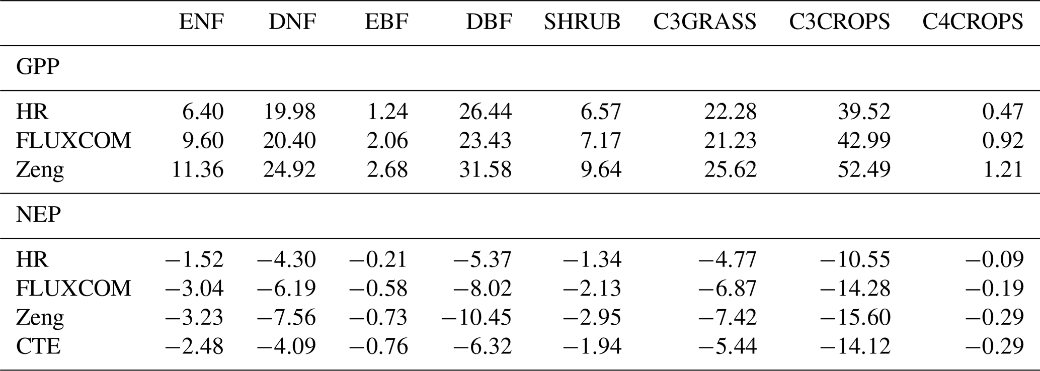
On the European scale, the SiB4 biosphere CO₂ fluxes have previously been compared to eddy covariance flux observations by, e.g., Smith et al. (2020) and Kooijmans et al. (2021) and show a good comparison (RMSE of roughly 2 $\mathrm{\mu }\mathrm{mol}{\mathrm{m}}^{-\mathrm{2}}{\mathrm{s}}^{-\mathrm{1}}$; Haynes et al., 2019). We also compared the PFT-aggregated mean of the NEP from both FLUXCOM and Zeng et al. (2020) to our CTE-HR product for the growing season (MJJA) of 2017. We find that both FLUXCOM and the product by Zeng et al. (2020) have a higher NEP than CTE-HR but that the latter might better agree with regional integrals. Table 7 shows the differences where the high NEP corresponds to earlier reports (Jung et al., 2020; Zeng et al., 2020) of large NEP (globally integrated near the 10 PgC yr⁻¹ sink in FLUXCOM). It also agrees with a tendency for EC-based analyses to represent high uptake locations rather than lower or average locations, leading to potential overestimates of the machine-learning-derived fluxes (Jung et al., 2020; Zeng et al., 2020). In contrast, fluxes optimized using data assimilation of atmospheric CO₂ mole fraction observations from among others the European ICOS network in CTE (Friedlingstein et al., 2022b) suggest a lower NEP, with the integral matched by CTE-HR more closely than the other products for most PFTs.

Our CTE-HR fluxes generally show a lower GPP compared to FLUXCOM (which arguably gives more reliable GPP than NEP estimates), especially for needleleaf ecosystems found in Scandinavia and for C₃ crops. The latter is a generic PFT in SiB4 and mostly used as a placeholder for specific crop species that are part of SiBCrop (Lokupitiya et al., 2009). The agreement with FLUXCOM is generally better than with Zeng et al. (2020), and CTE-HR typically is slightly low in GPP. Additionally, we compared biosphere fluxes of CTE-HR to eddy covariance flux observations to assess the mean error (ME), RMSE, and correlation coefficient (R) (Appendix B). The differences for both NEP and GPP are generally within the “local” error.

Table 7 Gross primary production (GPP) and net ecosystem productivity (NEP), integrated over the growing season (MJJA) of 2017 (TgC / month) for different land-use types (ENF: evergreen needleleaf forests; DNF: deciduous needleleaf forests; EBF: evergreen broadleaf forests; DBF: deciduous broadleaf forests; SHRUB: shrublands; C3GRASS: C₃ grasslands; C3ROPS: C₃ croplands; C4CROPS: C₄ croplands). The land-use types are taken from the CORINE dataset (Bossard et al., 2000). HR refers to the product described here, Zeng refers to the product as described by Zeng et al. (2020), FLUXCOM refers to the product by Jung et al. (2020), and CTE refers to NEP optimized using data assimilation of atmospheric CO₂ mole fraction observations (Friedlingstein et al., 2022b).

4.3 Atmospheric transport

Our transported CTE-HR fluxes show a better agreement with CO₂ mole fraction observations compared to a poor person's inversion, which is a relatively simple way of generating near-real-time flux estimates. In this comparison to observations, we used both the relatively coarse-resolution transport model TM5 (Krol et al., 2005) at 1×1^∘ for Europe as well as the high-resolution transport model STILT (Gerbig et al., 2003), driven by IFS meteorological fields at 0.1^∘ × 0.2^∘ for the Lutjewad tower in the Netherlands specifically. Using the high-resolution fluxes, we capture more variability compared to fluxes that are averaged to 1×1^∘ and fluxes that have no temporal profile. Moreover, the high resolution allows us to study the effect of individual sectors, highlighting emission hotspots, such as power plants, as a category that benefits most directly from high-resolution fluxes and high-resolution transport. As we found similar results for the Cabauw tower in the Netherlands (not shown), we speculate that, also for atmospheric CO₂ modeling at other European locations, the added resolution of the CTE-HR product will matter most for the specific wind directions and times of day when point sources contribute to the signal. Note that we assumed all emissions to be on the surface, which might bias stack emissions (Maier et al., 2022). Nevertheless, we do not expect this to influence the results of our comparison, as we assume this for the high-resolution fluxes, the 1×1^∘ fluxes and the flattened fluxes. The largest fraction of observed CO₂ variability however is driven by synoptic variations and biospheric fluxes, even in an emission-dense region in the Netherlands where we assessed the Lutjewad and Cabauw tower records. As a result, the use of high-resolution fluxes (or low-resolution transport, not shown) does not directly affect our skill in simulating atmospheric mole fractions. This indicates that atmospheric transport models should be improved at the sub-synoptic timescales to study high-resolution fluxes in more detail, for example, in their representation of the mixed layer height, as Lagrangian transport models are known to be sensitive to this.

The importance of atmospheric transport is also relevant for our analysis of the Amsterdam fluxes. We underestimate the fluxes, which we attribute to the small footprint of the flux tower, which is much smaller than the grid cells in our model (Nicolini et al., 2022). A minor contribution to the underestimation is that we do not account for human respiration in our model, which attributes roughly 3 % of the total CO₂ flux in urban areas (Ciais et al., 2020). However, our underestimation is larger than the possible effect of human respiration. Additionally, we do not account for biosphere fluxes in Amsterdam, as we only compare them to anthropogenic fluxes. In winter, biosphere fluxes are a source resulting in higher CO₂ emissions. In contrast, in summer, the biosphere acts as a sink, offsetting the positive anthropogenic flux. Thereby, the biosphere can explain part of the smaller underestimation of the Amsterdam fluxes in summer compared to winter. Although our simulated fluxes are lower than the observed fluxes, we find a very good correlation between simulated and observed diurnal cycles (R=0.94), indicating that we capture the time profile of emissions in Amsterdam well. To better capture the absolute fluxes as seen by the flux tower, we should create higher-resolution (<500 m) fluxes similar to the footprint of the flux tower. Although this is possible, it would be computationally expensive, and we deem 0.1 × 0.2^∘ to be high enough to use as a ready-to-use alternative for current European regional fluxes, especially given the limitations by current state-of-the-art transport models in urban environments.

4.4 Future outlook

Currently, CTE-HR provides biogenic, anthropogenic, ocean and wildfire CO₂ fluxes. However, for CO₂ emission verification, other tracers and isotopes can also be used (Balsamo et al., 2021), such as CO and NO₂ that are co-emitted with CO₂. CO and NO₂ column abundances can be monitored with satellites and have been used for monitoring and verification of high-resolution anthropogenic CO₂ fluxes (Konovalov et al., 2016; Reuter et al., 2019). For these co-emitted species, a differentiation between different power plants should be included, as different fuels have different emission ratios of CO₂, CO, and NO_x. For further improved MVS systems, biosphere fluxes should be disentangled from anthropogenic CO₂ fluxes. For this the radioactive isotope radiocarbon (¹⁴C) can be used (Levin et al., 2011; Miller et al., 2020; Basu et al., 2020). However, ¹⁴C samples have to be analyzed in a laboratory and therefore cannot be measured continuously or in near real time (Levin et al., 2020). Oxygen (O₂), on the other hand, does not have this drawback. Oxygen is exchanged during different plant processes and is consumed in the combustion of fossil fuels. By assessing O₂:CO₂ ratios, oxygen has previously been used to study the carbon budget of deciduous forests in the USA and Japan (Battle et al., 2019; Ishidoya et al., 2015) and to study the reduction of anthropogenic CO₂ emissions in the UK during the COVID-19 lockdown (Pickers et al., 2022). Furthermore, the isotopic signature Δ¹⁷O in CO₂ is suggested as a tracer for gross primary production (Hoag, 2005; Koren et al., 2019), and this tracer can also inform on the fossil fuel contribution to CO₂ mole fractions (Laskar et al., 2016). Measurements at the Lutjewad site are currently ongoing (Steur et al., 2021). To enable improved constraints on the European carbon budget, we aim to include estimates of the previously mentioned gases and isotopes in future releases. Measurements of these gases and satellite retrievals are generally available with a small latency (roughly 1 d, with the exception of the isotopes and oxygen) (e.g., https://doi.org/10.18160/ATM_NRT_CO2_CH4; ICOS Research Infrastructure, 2018) and can therefore be used for a near-real-time application as well.

With atmospheric CO₂ measurements being available within a few days, one might expect our flux product to have a similar latency. Currently, our latency of roughly 8 weeks is dominated by Eurostat statistical data and ERA5 meteorological data. Also, other flux products such as https://carbonmonitor.org and GRACED (Dou et al., 2021) have this limitation. In a future update we aim to create a more near-real-time emission estimate. With ENTSO-E data and ERA5 meteorological fields, we already have near-real-time information on public power and household emissions as well as biosphere and oceanic fluxes. For a more complete budget, near-real-time scaling of the other major sectors, on-road and industrial, should be included. Using near-real-time atmospheric data, atmospheric transport can also be made near real time. Operational transport of the near-real-time fluxes gives a continuous verification of our European carbon fluxes, and we aim to do this in a future release of this product.

4.5 Potential usage of CTE-HR

In contrast to other currently available near-real-time, high-resolution flux products, our fluxes are designed to be used as an easy substitute for less-informed or lower-resolution carbon flux products over Europe in modeling studies. CTE-HR is developed with the emphasis on estimating fossil fuel emissions and biosphere exchange rapidly, using information from emission proxies to estimate the recent state of European carbon exchange. Having noted this, it is not intended to be used as a policy tool directly, and generated fluxes are not a substitute for emissions reported by national emission registration entities.

5 Data availability

Fluxes generated by CTE-HR are available on the ICOS carbon portal https://doi.org/10.18160/20Z1-AYJ2 (van der Woude, 2022a). The fluxes contain modified Copernicus Atmosphere Monitoring Service Information (2022).

6 Code availability

The used code is available at https://doi.org/10.5281/zenodo.6477331 (Van Der Woude, 2022b), and a living repository can be found at https://git.wageningenur.nl/ctdas/CTDAS/-/tree/near-real-time (last access: 27 January 2023).

7 Conclusions

We demonstrate and validate our new framework for estimating high-resolution carbon fluxes over Europe: CTE-HR. Its fluxes are created with a latency of about 8 weeks, and we show here that they can readily be used in atmospheric (inverse) modeling frameworks. The CO₂ fluxes provided by CTE-HR are driven by information on socioeconomic activity and meteorological data as dynamical proxies for variability that is unresolved in static emission inventories. We show that our fluxes reflect recent anomalies in both the European biosphere and economic activity due to the 2018 drought and COVID-19 lockdowns well, and after atmospheric transport they result in satisfactory agreement with CO₂ observations at European measurement towers at the continental scale. Individual emission sectors are resolved at high resolution and can be separated into CO₂ mole fraction signals when transported to the Lutjewad tower in the Netherlands. The benefits of the high-resolution aspect of our CTE-HR fluxes are highest for the 5 %–10 % of observed signals that are dominated by point sources, mostly from energy production. At even smaller scales, our fluxes represent the temporal variations well, but our estimated flux magnitudes are too coarse to be used for urban-scale carbon flux studies.

The CTE-HR system is built into the CarbonTracker Data Assimilation Shell (CTDAS) system (Van der Laan-Luijkx et al., 2017), allowing flexibility and potential use in inverse modeling studies. Future developments include the addition of other species, reduced latency, improved representation of biosphere fluxes and (automated) transport of the fluxes through the atmosphere to have an operational, continuous comparison to atmospheric mole fractions. The CTE-HR flux products are available on the ICOS Carbon Portal (https://doi.org/10.18160/20Z1-AYJ2; van der Woude, 2022a), and we plan regular updates to stay within 2 months of real time.

Appendix A: ENTSO-E data

Figure A1 shows a specific case where the added information from the ENTSO-E data is valuable.

Figure A1 CO₂ emission from the energy sector, according to the ENTSO-E reported data and CTE-HR (blue line) and the CAMS-REG-GHG dataset (green line) over Germany for December 2017. The grey area indicates the period in which the negative energy prices occurred.

Appendix B: Uncertainty of the biosphere model

Table B1 Mean error (ME, $\mathrm{\mu }\mathrm{mol}{\mathrm{m}}^{-\mathrm{2}}{\mathrm{s}}^{-\mathrm{1}}$), root mean square error (RMSE, $\mathrm{\mu }\mathrm{mol}{\mathrm{m}}^{-\mathrm{2}}{\mathrm{s}}^{-\mathrm{1}}$) and Pearson's correlation coefficient (R) of daytime means (11–16 h) of the CTE-HR biosphere fluxes, compared to flux towers (N=17) at similar land-use types, for different seasons. The number provided is the median of the N sites per PFT (in parentheses).

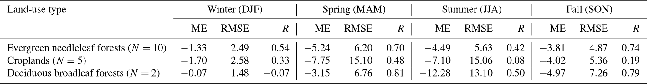
We compared the CTE-HR biosphere flux to the observed NEP at 16 flux towers, where the land-use class is similar to the plant functional type that we use for the downscaling. We analyze the daytime mean fluxes (between 11:00 and 16:00 local time). We assess the mean error (the bias), the root mean square error (RMSE), and the correlation coefficient (R). As these metrics vary over the year, we denote them per season. The 16 used towers are “SE-Htm”, “BE-Bra”, “FI-Hyy”, “DK-Vng”, “DE-RuS”, “SE-Svb”, “FR-Bil”, “DE-Tha”, “BE-Vie”, “FR-Fon”, “SE-Nor”, “CH-Dav”, “DE-Geb”, “DE-HoH”, “BE-Lon”, “FR-Lam”, and “IT-SR2” (Arriga et al., 2022; Brut et al., 2022; Heinesch et al., 2022; Rebmann et al., 2022; Bruemmer et al., 2022; Buchmann et al., 2022; Mölder et al., 2022; Dufrêne et al., 2022; Vincke et al., 2022; Bernhofer et al., 2022; Loustau et al., 2022; Peichl et al., 2022; Schmidt et al., 2022; Friborg et al., 2022; Mammarella et al., 2022; Janssens et al., 2022; Heliasz et al., 2022).

We compare our flux estimates at a specific grid cell to flux towers, which shows the expected mismatch when comparing our biosphere fluxes to eddy covariance towers. As the used metrics vary over the year, we denote them per season in Table B1.

Note that we compare our 0.1^∘ × 0.2^∘ grid cells here to often pristine eddy covariance sites.