Spatiotemporally resolved emissions and concentrations of styrene, benzene, toluene, ethylbenzene, and xylenes (SBTEX) in the US Gulf region

Styrene, benzene, toluene, ethylbenzene, and xylenes (SBTEX) are established neurotoxicants. SBTEX contains hazardous air pollutants (HAPs) that are released from the petrochemical industry, combustion process, transport emission, and solvent usage sources. Although several SBTEX toxic assessment studies have been conducted, they have mainly relied on ambient measurements to estimate exposure and limit their scope to specific locations and observational periods. To overcome these spatiotemporal limitations, an air quality modeling system over the US Gulf region was created, predicting the spatially and temporally enhanced SBTEX modeling concentrations from May to September 2012. Due to the incompleteness of SBTEX in the official US Environmental Protection Agency (EPA) National Emission Inventory (NEI), the Hazardous Air Pollutions Imputation (HAPI) program was used to identify and estimate the missing HAP emissions. The improved emission data were processed to generate the chemically speciated hourly gridded emission inputs for the Comprehensive Air Quality Model with Extensions (CAMx) chemical transport model to simulate the SBTEX concentrations over the Gulf modeling region. SBTEX pollutants were modeled using the Reactive Tracer feature in CAMx that accounts for their chemical and physical processes in the atmosphere. The data show that the major SBTEX emissions in this region are contributed by mobile emissions (45 %), wildfire (30 %), and industry (26 %). Most SBTEX emissions are emitted during daytime hours (local time 14:00–17:00), and the emission rate in the model domain is about 20–40 t h⁻¹, which is about 4 times higher than that in the nighttime (local time 24:00–04:00, about 4–10 t h⁻¹). High concentrations of SBTEX (above 1 ppb) occurred near the cities close to the I-10 interstate highway (Houston, Beaumont, Lake Charles, Lafayette, Baton Rouge, New Orleans, and Mobile) and other metropolitan cities (Shreveport and Dallas). High styrene concentrations were co-located with industrial sources, which contribute the most to the styrene emissions. The HAPI program successfully estimated missing emissions of styrene from the chemical industry. The change increased total styrene emissions by 22 %, resulting in maximum ambient concentrations increasing from 0.035 to 1.75 ppb across the model domain. The predicted SBTEX concentrations with imputed emissions present good agreement with observational data, with a correlation coefficient (R) of 0.75 (0.46 to 0.77 for individual SBTEX species) and a normalized mean bias (NMB) of −5.6 % (−24.9 % to 32.1 % for the individual SBTEX species), suggesting their value for supporting any SBTEX-related human health studies in the Gulf region. The SBTEX data were published at Zenodo (https://doi.org/10.5281/zenodo.7967541) (Wang et al., 2023), and the HAPI tool was also published at Zenodo (https://doi.org/10.5281/zenodo.7987106) (Wang and Baek, 2023).

1 Introduction

Styrene, benzene, toluene, ethylbenzene, and xylenes (SBTEX) are listed as hazardous air pollutants (HAPs) by the US Environmental Protection Agency (EPA) (Declet-Barreto et al., 2020) and can be detected in unhealthy amounts in the ambient environment. SBTEX are primarily from industrial emission sources and can be found in the petrochemical, construction, and manufacturing industries (Polvara et al., 2021; Declet-Barreto et al., 2020), with 98 % of the benzene emissions attributed to coal and petroleum sources (ATSDR, 2007a, b, 2010a, b, 2017). Exposure studies of the total SBTEX at industrial sources in the Middle East, Europe, and western Asia have shown that workers experience a cumulative yearly environmental exposure of 25–176 ppb (Al-Harbi et al., 2020; Rajabi et al., 2020; Christensen et al., 2018; Rahimpoor et al., 2022; Niaz et al., 2015; Moshiran et al., 2021). The inhalation reference concentration for benzene shows low-dose linearity utilizing a maximum likelihood estimate E-5 risk level of benzene (1 in 100 000); the range is 0.4–1.4 ppb of the air concentration for leukemia (USEPA, 2000).

Given the importance of SBTEX from industrial sources, the heavily industrialized Gulf region of the US could be a significant source of exposure for the population living there. According to the Agency for Toxic Substances and Disease Registry (ATSDR) report, the petrochemical industry in the Gulf region states contributes approximately 52 % (∼5.3 million t yr⁻¹) of benzene production capacity in the US (ATSDR, 2007a) and ∼75 % (∼ 6.2 million t yr⁻¹) of xylene production capacity (ATSDR, 2007b). Texas and Louisiana have significant production of styrene and ethylbenzene, with annual productions of 5.5 and 7.2 million t yr⁻¹, respectively (ATSDR, 2010a). A recent study of SBTEX exposures in the US Gulf region, conducted within the Gulf Long-term Follow-up Study (GULF Study) cohort (NIEHS, 2021), observed associations of blood concentrations and annual average air concentrations of these chemicals with neurological symptoms (Werder et al., 2019, 2018). The average blood BTEX concentration among the 146 tobacco-smoke-unexposed participants with blood measurements in this study was 255 ng L⁻¹ (Doherty et al., 2017; Werder et al., 2018). This value is similar to that for a representative nationwide sample assessed as part of the US National Health and Nutrition Examination Survey (NHANES) in 2005–2008 (NCHS, 2021), which measured an average of 247 ng L⁻¹. In GULF Study, however, the 95th percentile of the BTEX concentrations was 991 ng L⁻¹, which is 23 % higher than the 95th percentile for the NHANES nationwide sample of 803 ng L⁻¹. The mean blood concentration of styrene for the GULF Study sample was 52 ng L⁻¹ (95th percentile: 882 ng L⁻¹) or twice the NHANES nationwide mean of 25 ng L⁻¹ (95th percentile: 55 ng L⁻¹) (NCHS, 2021). Due to the short biological half-lives of SBTEX species, the study concluded that this high average SBTEX concentration in blood in the Gulf region resulted from recent, presumably local, emission sources.

Most ambient exposure studies of SBTEX have relied directly on local measurements from the field or at existing ambient monitors. These measurements can then be used in statistical models to spatially predict exposures to SBTEX (Pankow et al., 2003; O'Leary and Lemke, 2014; Miller et al., 2018; Hsieh et al., 2020). For example, Hsieh et al. (2020) developed multivariate linear regression (MLR) models to estimate SBTEX concentrations using correlations with other criteria air pollutants, including nitrogen oxides (NO_x), carbon monoxide (CO), sulfur dioxide (SO₂), particulate matter (PM), and meteorological conditions (temperature, wind speed). The MLR model predicted a strong correlation with NO_x and CO. The limitations of the statistical model are that they require measurement data, and they assume that the measurements originate from a single source in a relatively small region. The use of a dispersion model is another way of estimatinng ambient SBTEX concentrations when local measurements are lacking. Chen et al. (2016) applied a dispersion model to predict SBTEX and other toxicant concentrations in two industrial complexes in Kaohsiung, Taiwan. The dispersion model performed better for stationary point sources than a statistically based model and predicted up to ∼78 % of the ambient observation. These dispersion models, however, only account for exposures at a smaller spatial scale (USEPA, 2022, 2023) and thus cannot support regional-scale (e.g., state-level) application. Furthermore, these models assumed that the exposure rate to SBTEX is linear without considering any chemical destruction and wet or dry deposition losses in the atmosphere.

An accurate SBTEX assessment in the Gulf region must address the known uncertainties associated with current statistical, biometric, and dispersion model approaches. Improved accuracy in exposure estimation is dependent on the inclusion of all industrial emission sources, must capture the temporal and spatial variability known to occur in industrial emission rates, and should include the chemical and physical decay processes of the atmosphere. These issues can be addressed using a regional-scale chemical transport model (CTM), like the Comprehensive Air Quality Model with Extension (CAMx) (Ramboll, 2021) coupled with an emission inventory that provides a comprehensive account of all the SBTEX sources. In addition, the Reactive Tracer function, which is one of the CAMx probing tools, allows the model to explicitly simulate SBTEX concentrations. Currently, SBTEX emission data can be found in the EPA's National Emission Inventory (NEI), which includes data from the Toxics Release Inventory (TRI) program database (USEPA, 2021d). Unlike for benzene sources, the TRI data for the other four species (STEX) are based on voluntary reports, and as a result, the 2011 NEI has emission rate data for these air toxicants only for a limited set of emission sources (USEPA, 2021a).

The following work describes the development of a new STEX emission inventory for the Gulf Coast region that includes the emission sources absent from the 2011 NEI. Missing emission rate data of STEX were provided by analyzing NEI emissions of similar industrial sources that did provide emission rates and by applying their rates to the missing source. Diurnal profiles for STEX were based on the hourly profiles of other pollutants with the same type of industrial source. This study then applied the Sparse Matrix Operator Kernel Emissions (SMOKE) model system (Baek and Seppanen, 2021) to generate a CAMx-ready emission inventory. Since STEX is not included as an explicit species in the chemical mechanisms used by CAMx, a reactive tracer was included to account for chemical losses. This new emission inventory was then utilized in CAMx to predict STEX concentrations over the Gulf region for 5 months in 2012.

2 Materials and methods

In this study, the 2011 version 6 NEI was applied as the base emission inventory (USEPA, 2021b). Subsequently, the SMOKE modeling system was employed to produce hourly gridded emissions of SBTEX across the Gulf modeling region for the year 2012. These SBTEX emissions were utilized in conjunction with the CTM and a reactive tracer function to generate the SBTEX concentration map. In the end, the US EPA Ambient Monitoring Technology Information Center (AMTIC) data were employed to evaluate the model performance in simulating SBTEX concentrations.

2.1 Emission data preparation

2.1.1 The HAP emissions into the NEI

The NEI is a national database providing comprehensive annual air emission estimates for both criteria air pollutants (CAPs) (e.g., CO, NO_x, SO₂, NH₃, VOC, and PM_2.5) and HAPs (e.g., benzene, acetaldehyde, formaldehyde, xylenes, and styrene) from all types of emission sources (e.g., point, nonpoint, and mobile). While CAP emissions being reported by state agencies is mandatory, the report of HAPs is usually voluntary. Consequently, only a limited set of HAPs has been reported to the US EPA, and their spatial coverage can vary significantly by source type (e.g., industrial, vehicles) and region (e.g., county, state) (Strum et al., 2017).

The VOC emission species generated by SMOKE from the NEI have three types, which are “model surrogate”, “model-explicit”, and “HAP-explicit” species. The model surrogate species, such as XYL (xylene and other poly-alkyl aromatics), TOL (toluene and other mono-alkyl aromatics), and PAR (paraffin carbon bond), are calculated by speciation profiles in the emission model platform and are used to predict ozone and secondary organic aerosol (SOA) in the CTM but not for individual HAP emissions and simulations. Only five HAP emissions in the NEI are model-explicit species: naphthalene (NAPH), benzene (BENZ), acetaldehyde (ALD2), formaldehyde (FORM), and methanol (MEOH), which are known as “NBAFM” to represent their individual emission (Strum et al., 2017) and are directly processed in the CTM too. The HAP-explicit species emission in the NEI includes hundreds of toxicants (such as styrene, xylenes, mercury, and acrolein). Those HAP-explicit species cannot be directly used in the current CTM because their explicit chemical mechanisms are not developed in the current CTM chemical mechanism.

The model-explicit species, benzene (B), and other HAP-explicit species, including STEX, are targeted for this SBTEX human exposure study. The SMOKE model system (Baek and Seppanen, 2021) assigned the annual or monthly SBTEX emission inventory in the NEI to hourly emission patterns by the temporal profiles based on emission processes and locations by the Source Category Code (SCC) and the Federal Information Processing Standards (FIPS) county codes. These processes are coupled with the CAPs when generating the CTM-ready emission data.

2.1.2 Imputation of the NEI with STEX

Considering that benzene emission reporting is mandatory in the NEI and thus can be assumed to have no significant missing sources, we only focused on the investigation of missing sources for the STEX, which is voluntary reporting. This study utilized the 2011 NEI summary reports from the SMOKE modeling system (Baek and Seppanen, 2021) to identify those missing STEX emission sources. The SMOKE reports provided the annual or monthly total of VOC and individual HAP emissions sorted by the SCC and FIPS county codes. This study developed an R project (R Foundation, 2021) program called Hazardous Air Pollutants Imputation (HAPI) that can first read the reports from SMOKE and identify the list of inventory sources reported without STEX toxicants. Then it generated the imputation data for those missing STEX inventory sources based on the proxy of STEX and VOC for those emission sources that share the same SCC near the region (county or state).

Theoretically, the SCC is the reference code defining the emission process type. The same SCC means they share similar emission factors with the same emission process (USEPA, 2016). The profiles of HAPs for the VOC can be shared with those same SCC emission sources within the surrounding regions (counties or states) (Strum et al., 2017). When there are the same SCC emission sources with zero HAPs in other counties, this study performed the imputation of those missing HAP emissions based on the HAP profiles from the matched emission source. For example, the HAP profile of styrene and toluene in the VOC emission is defined as the ratio of styrene and toluene emissions over the VOC emission (P_toluene,s) in counties where there are styrene, toluene, and VOC emissions for that SCC (s). Then, this study will assume that those HAPs are missing when the summation of HAP emissions is zero ($\sum _i{E}_{i,\mathrm{s},\mathrm{f}}=\mathrm{0}$: i is pollutants, “s” is the SCC code, and “f” is the FIPS county code), but the VOC emission is available. Then this will apply the HAP profile for the same SCC to the existing VOCs and estimate missing styrene and toluene emissions. Therefore, this process can impute the missing HAP emissions based on the SCC-matched HAP fractions from the surrounding counties or the same state.

The HAPI was developed based on this imputation concept. This study first separated the county and SCC level inventory data into two groups in the HAPI program: “with HAPs” and “without HAPs”. For the “with HAPs” group, summations of HAP emissions in counties and SCCs are not zero. In contrast, for the “without HAPs” group, summations of HAP emissions in counties and SCCs are zero.

In the “with HAPs” group ($\sum _i{E}_{i,\mathrm{s},\mathrm{f}}>\mathrm{0}$) in Eq. (1), i is the individual HAP, such as styrene, benzene, toluene, ethylbenzene, xylenes, acrolein, and 1,3-butadiene; “s” is the SCC, and “f” is the county FIPS code for the county. $E_{i,\mathrm{s},\mathrm{f}}$ is the annual emission of the pollutant i for the SCCs in the county. $E_{\mathrm{voc},\mathrm{s},\mathrm{f}}$ is the CAP VOC emission for the SCCs in the county. The HAP profile (P_i,s) is a fraction of the HAP-specific emission ($E_{i,\mathrm{s},\mathrm{f}}$) over the summation of the matched SCC and county-specific VOC emissions ($E_{\mathrm{voc},\mathrm{s},\mathrm{f}}$) from the “with HAPs” group.

This study assumed that, if there is an SCC-matched “with HAPs” HAP profile in the inventory, they are not considered missing HAP emission sources. Only the emission sources for which the sum of all the HAPs is zero ($\sum _i{E}_{i,\mathrm{s},\mathrm{f}}=\mathrm{0}$) are considered the “without HAPs” group. In Eq. (2), P_i,s is used to estimate those missing HAPs for the “without HAPs” inventory source group. $E_{\mathrm{voc},\mathrm{s},\mathrm{f}}$ is the CAP VOC emission in the “without HAPs” group.

When $\sum _i{E}_{i,\mathrm{s},\mathrm{f}}>\mathrm{0}$, calculate individual HAPs to the total VOC ratio (P_i,s):

$$\begin{array}{}\text{(1)}& P_{i,\mathrm{s}}={\displaystyle \frac{\sum _f{E}_{i,\mathrm{s},\mathrm{f}}}{\sum _f{E}_{\mathrm{voc},\mathrm{s},\mathrm{f}}}}.\end{array}$$

When $\sum _i{E}_{i,\mathrm{s},\mathrm{f}}=\mathrm{0}$, the HAP emissions are missing. This study applied P_i,s and VOC emission to estimate the missing HAP emission:

$$\begin{array}{}\text{(2)}& {\text{Em}}_{i,\mathrm{s},\mathrm{f}}=P_{i,\mathrm{s}}\times E_{\mathrm{voc},\mathrm{s},\mathrm{f}}.\end{array}$$

The HAPI program then outputs the total HAP emissions (Em${}_{i,\mathrm{s},\mathrm{f}}$) for the SMOKE modeling system to integrate with the CAP VOC inventory described in Sect. 2.1.2. Finally, the HAPI program performs the quality-assurance step again to confirm that there are no missing HAPs after imputation and that the summation of HAP emissions is not greater than the CAP VOC emission.

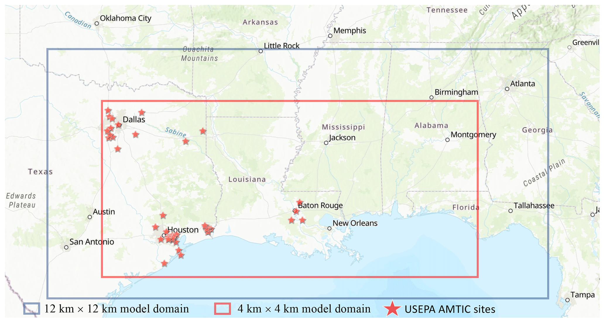
Figure 1 The modeling domains with the outer 12×12 km resolution domain (blue rectangle) and the inner 4×4 km resolution domain (red rectangle). The red stars are the US EPA Ambient Monitoring Technology Information Center (AMTIC) observational sites for hazardous air pollutants (HAPs). There are 4 sites in Louisiana and 42 sites in Texas. Generated with an ArcGIS map (Esri, 2013).

2.2 Model configuration

2.2.1 Air quality modeling

The Comprehensive Air Quality Model with Extensions version 7.0, CAMx7.0 (Ramboll, 2020b), was implemented in this study to simulate the SBTEX concentrations in the atmosphere. The model simulation period is from 20 April to 30 September 2012 (20 to 30 April are spinup dates). The evaluated meteorological data from WRF version 3.8 over the US continental region are provided by the US EPA Support Center for Regulatory Atmospheric Modeling (SCRAM) (USEPA, 2022). The WRF output data were transformed into SMOKE-ready gridded hourly meteorology through the Meteorology Chemistry Interface Processor (MCIP). The emission sectors modulated by meteorology, such as on-road (Choi et al., 2014; Lindhjem et al., 2004) and biogenic, were estimated with the MCIP gridded hourly meteorology. The US EPA's 2012 daily total wildfire emissions (ptfire) estimated by SMARTFIRE2 (USEPA, 2015) were also incorporated (USEPA, 2021b). Additionally, the WRF meteorological data were converted to CAMx-ready meteorological data by using WRFCAMx (Ramboll, 2020b) for the CAMx model input. The photodissociation coefficients are calculated by the Tropospheric Ultraviolet-Visible (TUV) radiation model (Madronich, 1987) with Ozone Monitoring Instrument (OMI) daily data (NASA, 2023). The US EPA daily hemisphere CMAQ model results are used to calculate the boundary condition and initial condition (Hogrefe et al., 2021). The chemical mechanism is Carbon Bond 06 revision 4 (CB6r4) (Ramboll, 2020a). Figure 1 in the paper shows that the model domain is 12 km × 12 km (blue rectangle). We also created a 4 km × 4 km (red rectangle) nesting simulation to enhance the model spatial resolution through the flexi-nesting method. The point source emissions are processed independently with their stack locations in the model domain and considering the plume-raising effect by stack parameters. As a result, the model spatial allocations can be enhanced through the flexi-nesting method.

The modeling ozone evaluation results over the simulation period are shown in Table S2. The evaluation indicators followed the US EPA's model evaluation guidance (USEPA, 2006). The modeling ozone is performed fairly well over the Gulf Region's states (correlation coefficient (R) ≥0.55). The simulated ozones in Texas and Louisiana are close to the observation data in the US EPA AQS stations (Texas: R=0.79, normalized mean bias NMB = 1 %; Louisiana: R=0.77, NMB = 11 %). Additionally, because our model shares the same simulation period as the Texas Commission on Environmental Quality (TCEQ) 2012 Ozone State Implementation Plan (SIP) modeling application (TCEQ, 2016), we verified our modeling results with the TCEQ's simulated OH radical-related model species, including O₃, NO₂, and formaldehyde over the Dallas and Houston region (Fig. S2). The detailed comparisons are shown in the Supplement and indicate that both modeling applications share a similar, good modeling performance.

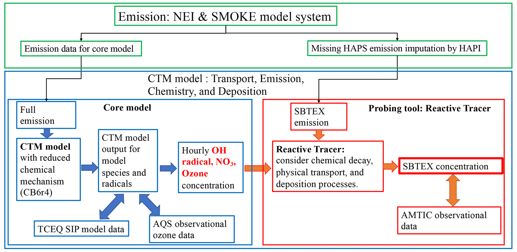
Figure 2 Toxic air quality modeling system schematic. The green rectangles are emission processes. The blue rectangles are the base CTM process for estimating the concentration of oxidants. The red rectangles are the Reactive Tracer process for estimating individual SBTEX concentrations.

2.2.2 Reactive Tracer

The overall research method scheme flowchart is shown in Fig. 2. After developing the CTM-ready emissions and the CAMx model for oxidant species (OH, O₃, and NO₃), the Reactive Tracer (RTRAC) was used to simulate the ambient SBTEX concentration over the Gulf region. The RTRAC is a probing tool in the CAMx modeling system to simulate explicit SBTEX concentrations. Along with the physical transport processes (diffusion and advection) and decay processes like wet and dry deposition, the same as in the core model, there is the second-order chemical reduction rate r that is calculated using the oxidant (ozone, OH, NO₃) concentrations [Ox], the SBTEX concentrations [Tr], and the rate constants of reactions k_Tr+Ox (Eq. 3). In Eq. (4), k is the rate constant calculated by A, B, temperature (T) and activation energy (E_a). The Master Chemical Mechanism for aromatic schemes (Bloss et al., 2005) is considered for the parameters of each specific reaction in the RTRAC process.

This study considered the initial reactions of SBTEX in the MCM version 3.3.1 (Jenkin et al., 2015). For the other parameters, the National Institute of Standards and Technology (NIST) Chemistry Webbook (Linstrom and Mallard, 2018) and the CAMx user guide (Ramboll, 2020b) are considered for determining the Henry's law constant, dependence temperature, and molecular weight. All the parameters used in our RTRAC modeling are presented in Tables S3 and S4.

$$\begin{array}{}\text{(3)}& {\displaystyle }r=k_{\mathrm{Tr}+\mathrm{Ox}}\left[\text{Tr}\right]\left[\text{Ox}\right]\text{(4)}& {\displaystyle }k=A{\left({\displaystyle \frac{T}{\mathrm{300}}}\right)}^B\exp \left({\displaystyle \frac{-E_{\mathrm{a}}}{T}}\right)\end{array}$$

The simulated SBTEX concentration will be evaluated by comparing it against observational data which will be described in the following.

Ambient SBTEX measurements

The CAMx modeling evaluation was completed with the US EPA Air Quality Station (AQS) ozone observational data and the TCEQ SIP ozone modeling output data (TCEQ, 2015). The measured ambient SBTEX concentrations are from the US EPA AMTIC, which is an observational network that routinely detects more than 100 air toxicants in the US (USEPA, 2021c). It includes the federal and state monitoring stations. The 5-month (May to September 2012) individual SBTEX concentrations from the AMTIC were utilized to evaluate the RTRAC modeling results from CAMx.

A total of 46 monitoring sites measure SBTEX concentrations within our 4 km × 4 km model domain, and most of them are located within Texas (42 sites), except for 4 sites in Louisiana. The air sampling duration can be 1, 3, or 24 h. There are six monitoring sites with 1 h measurement data in Texas, three sites with 3 h data in Louisiana, and the rest have 24 h data. The AMTIC sites are indicated in Fig. 1 with red stars. The US EPA conducted quality assurance or quality control for the AMTIC data, which contain values that are exceptionally high due to unpredictable industrial VOC release events (Couzo et al., 2012). These events are beyond the regulatory emission counting; thus, the model cannot capture those unpredictable events, particularly in petrochemical, oil, and gas industrial areas. Therefore, this study removed outliers (those beyond twice the interquartile range – IQR – above third quartiles – Q3) to better evaluate the model performance in simulating the SBTEX concentration in general.

The CAMx RTRAC modeling results are spatially and temporally resolved gridded hourly concentrations, while the AMTIC observational data are from specific locations with time gaps. Daily average and diurnal pattern analyses evaluate the predicted SBTEX concentrations. For each AMTIC site, this study used the average concentration of the center grid cell and eight other “surrounding” grid cells (i.e., the average of 3×3 grid cells) for comparison with the observational data (USEPA, 2006).

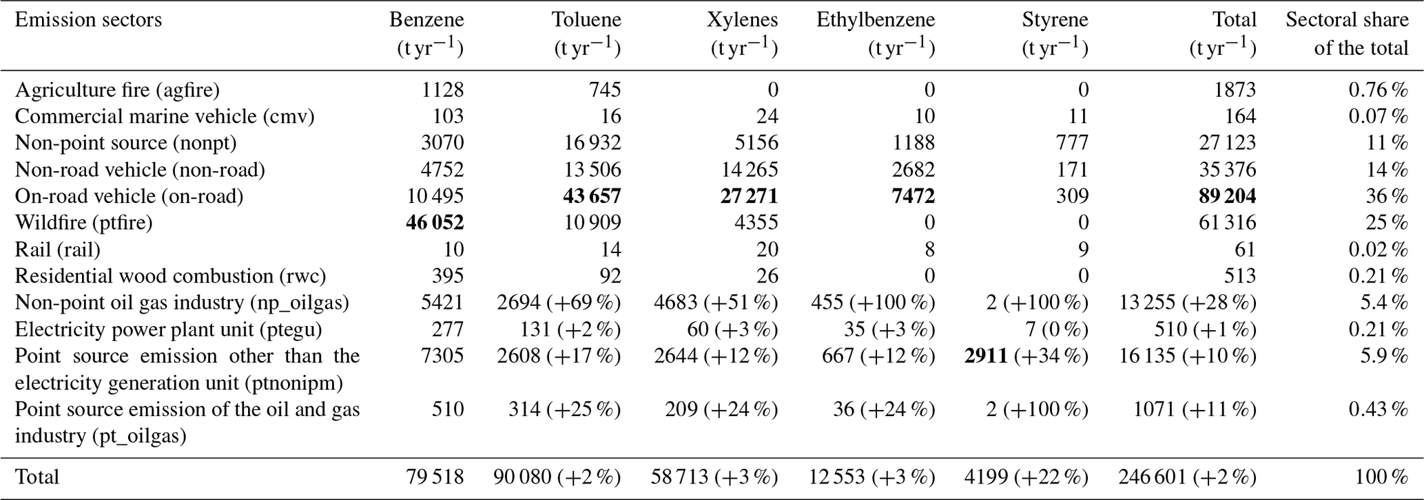
Table 1 The annual emission rates (metric tons yr⁻¹) of styrene, benzene, toluene, ethylbenzene, and xylenes (SBTEX) in 2012, including the increases resulting from this work. The percent increase from the 2012 National Emission Inventory is given in parentheses. The bold font indicates the emission sector with the maximum SBTEX rates.

3 Results

3.1 SBTEX emissions

The 2012 annual total SBTEX emissions in the model domain are shown in Table 1. The emission sectors include agriculture fire (afgire), commercial marine vessel (cmv), non-point source (nonpt), non-road vehicle (non-road), on-road vehicle (on-road), fire emission (ptfire), rail road (rail), residential wood combustion (rwc), non-point oil gas industry (np_oilgas), electricity power plant unit (ptegu), point source emission other than the electricity generation unit (ptnonipm), and the point source of the oil and gas industry (pt_oilgas). The largest contributor of SBTEX emissions in the 12 km × 12 km model domain is indicated as being from the “on-road” sector, with 89 204 t yr⁻¹ representing about 36 % of the total SBTEX emissions. The on-road sector contributes most to the total xylenes (46 %), toluene (48 %), and ethylbenzene (60 %) emissions but much less to benzene (13 %) and styrene (6.8 %). The second largest contributor to the SBTEX emissions is the “wildfire” sector (61 316 t yr⁻¹), contributing about 25 % of the total SBTEX. The wildfire contributes most of the total benzene (57 %), 12 % of the total toluene and 7 % of the total xylenes but no ethylbenzene and styrene due to the missing explicit profiles in the 2012 wildfire emission inventory. The “non-road” sector ranked third (35 375 t yr⁻¹), contributing about 14 % of the total SBTEX over our modeling region. Non-road contributes largely to xylenes (15 %), toluene (21 %), and ethylbenzene (21 %). Compared to the other sectors, emissions from non-electricity generation unit industrial point sources (ptnonipm) contain a larger portion of styrene, 2911 t yr⁻¹, which is 69 % of the total styrene emission. Our study successfully identified missing styrene emissions from the chemical industry process (see Table S7), leading to a 34 % increase in the total styrene emissions.

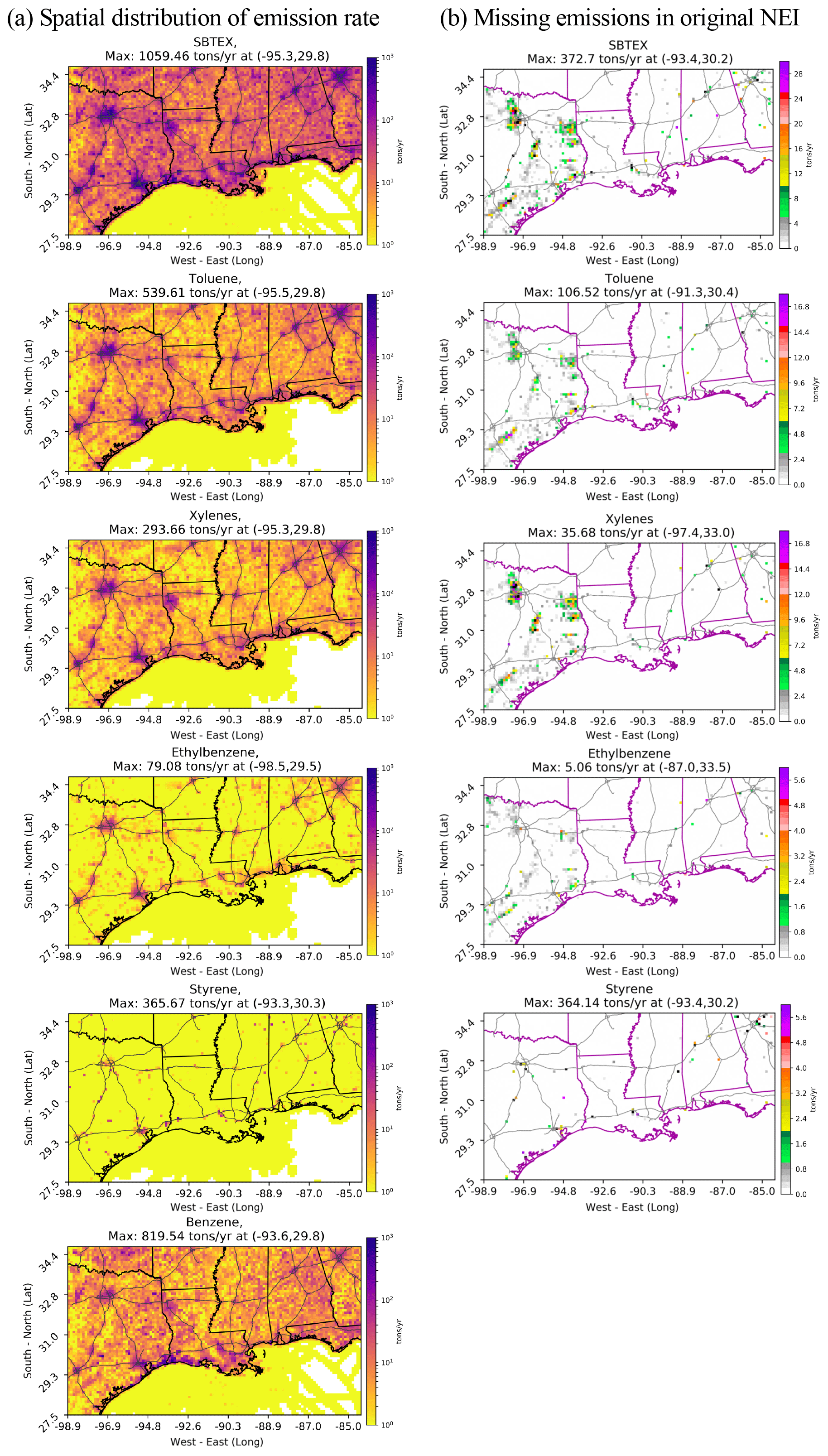
Figure 3 Spatial distribution of the 2012 annual total SBTEX emission rates (t yr⁻¹) of the modified emission inventory used in this work (a) and the location and amount of emissions that were added to the NEI (b).

The individual and total SBTEX annual emission spatial plots in the 12 km × 12 km model domain are presented in Fig. 3. The grid cell with the highest SBTEX emissions is found in Houston near the ship channel (1059 t yr⁻¹), which is about 35 times higher than the average emission (28 t yr⁻¹) across the domain, followed by one in San Antonio in Texas (1022 t yr⁻¹) and one near Sabine Lake in Louisiana (1022 t yr⁻¹). In Fig. 3b, the missing sources of SBTEX emissions in the NEI are mostly located in Texas and Louisiana, particularly for the grid cells in Lake Charles (increased by 373 t yr⁻¹, +282 %) and Baton Rouge (167 t yr⁻¹, +31 %) in Louisiana; Belton (61 t yr⁻¹, +21 %), Fort Worth (50 t yr⁻¹, +85 %), and Dallas (44 t yr⁻¹, +52 %) in Texas; and some rural areas in Texas. These missing sources of SBTEX are mostly from the np_oilgas and ptnonipm emission sectors (detailed in Supplement Sect. S3.1 and S3.2). Although the total SBTEX emission increased by only 2 % based on the domain average (Table 1), the localized impacts for certain areas can be up to 60 % of the total SBTEX emissions.

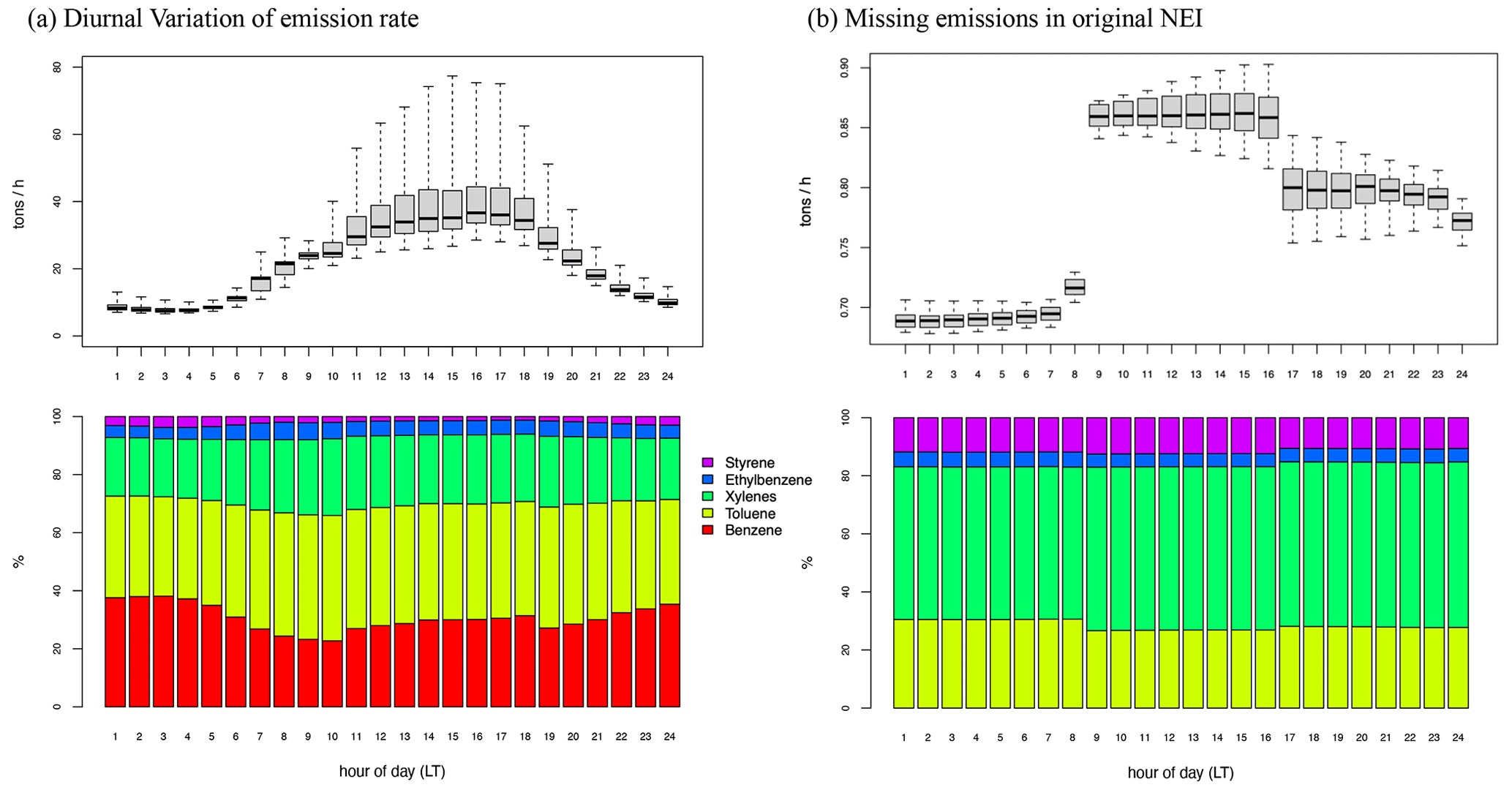
Figure 4 Diurnal emission pattern (a) and missing emission in the NEI (b) of the sum of SBTEX (domain total, t h⁻¹) (upper panel) and the average relative composition of five species (lower panel).

The SBTEX emissions exhibit strong diurnal variations across a day, as presented in Fig. 4a. The daytime hourly emission (up to 77 t h⁻¹) is about 4.3 times higher than the nighttime emission rate, mainly due to the larger emissions from on-road and off-road mobile sources (half of the total emissions) during the daytime. The diurnal variations in the chemical composition of the total SBTEX also suggested the increased percentages of toluene and xylenes (indicating the transport sources) during the morning (06:00–10:00 LT) and evening (19:00 LT) rush hours. The inclusion of the missing sources will slightly reduce the emission variation across a day, as most of the missing sources come from industrial manufacturing and oil processes (detailed in the Supplement), whose diurnal profiles are much flatter (about only a 20 % increase during the daytime) compared to the total emission (see Fig. 4b), with much smaller differences between the day (0.86 t h⁻¹) and night (0.69 t h⁻¹). The chemical compositions of the missing emission sources were relatively constant throughout the day, with about 50 % comprised of xylenes, 30 % of toluene, and 10 %–15 % of styrene. The relative amount of missing styrene was higher than that found in the total emissions.

3.2 Model performance

CAMx simulations predicting SBTEX concentrations were completed using two sets of emissions: the National Emission Inventory (“Base”) and the emission scenario adjusted in this study (“Adj”). The differences between the two scenarios can be regarded as impacts of the missing emission sources in the original NEI, suggesting the importance of the completeness of emissions.

Table 2 Normalized mean bias (NMB, %) and correlation coefficient (R) comparison of the average observational data and model result during the model simulation period, 1 May 2012 to 30 September 2012, for the 2012 National Emission Inventory (“Base”) and the emission scenario adjusted in this study (“Adj”). Bold font indicates the model improvement. Also shown is the count (N) of the available daily average data across all the sites.

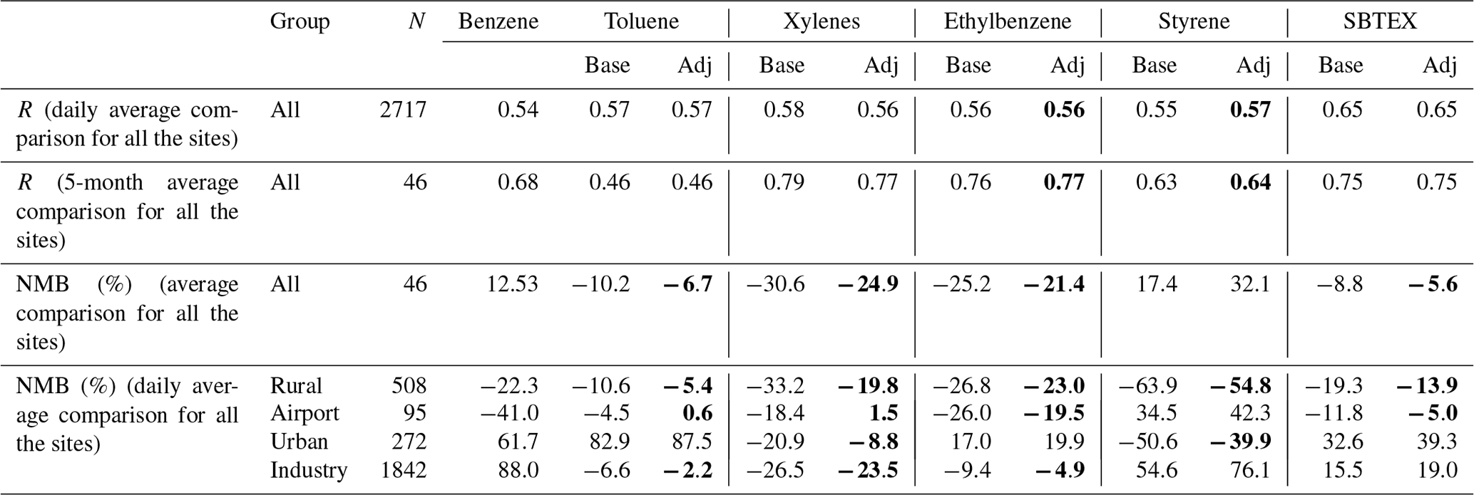
The simulated concentrations were compared with the observations to evaluate the accuracy of the SBTEX emissions and concentrations estimated in this study. The NMB (%) and correlation coefficient (R) of both the Base and Adj cases are compared in Table 2. Overall, the CAMx model can capture the pollution level and spatiotemporal variation of all the SBTEX species. More specifically, the model reproduced the daily variation of SBTEX concentrations, with R 0.65 (0.54–0.65 for individual SBTEXs) for all the daily observational records (N=2717) as well as their spatial distribution across the observational sites (N=46, averages of the whole simulation period), with R 0.75 (0.46 to 0.77 for the individual SBTEX species) and NMB −5.6 % (−24.9 % to 32.1 % for the individual SBTEX species).

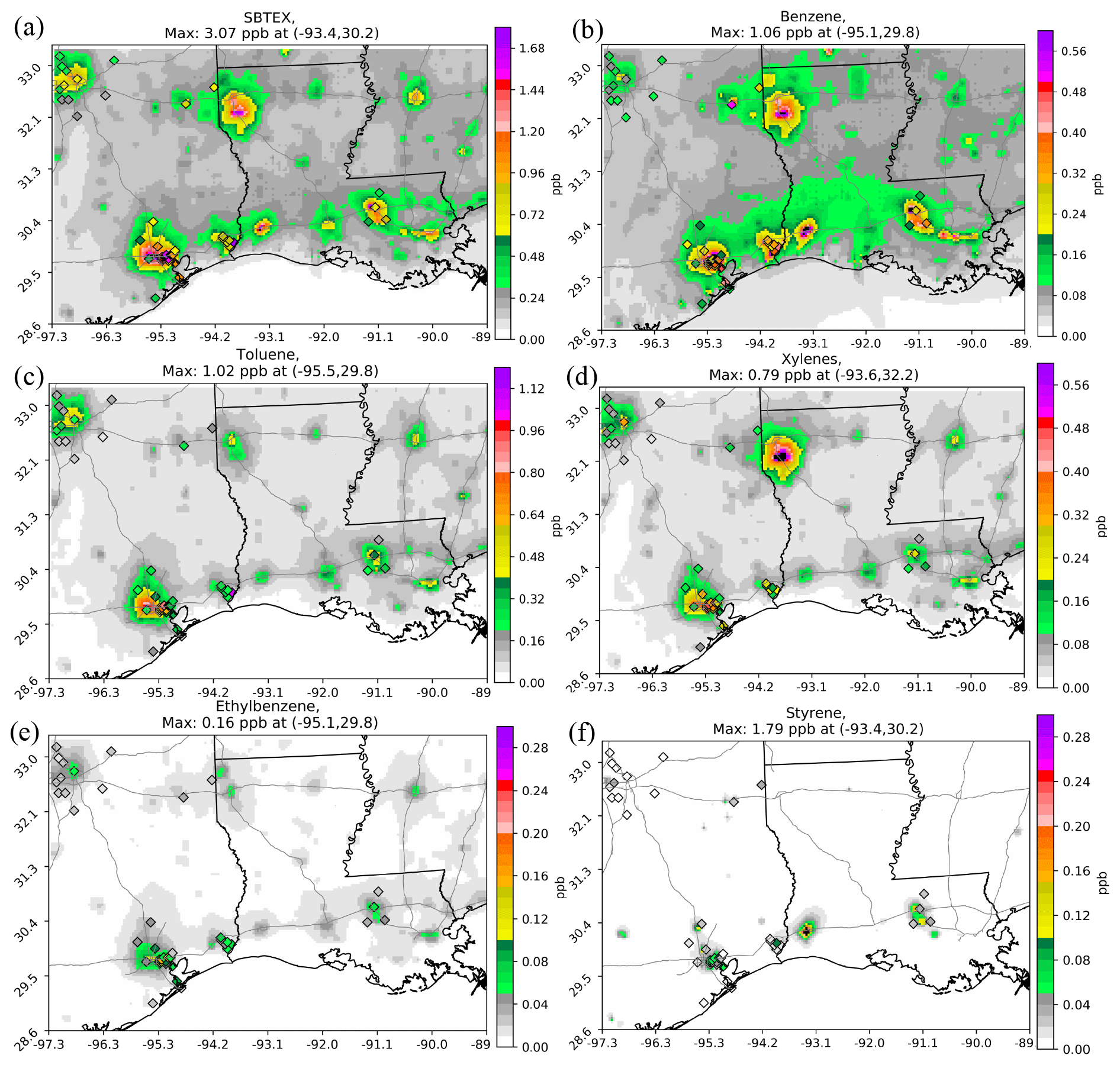
Figure 5 (a) The average concentration in the Adj scenario overlapped the average observational measurement data (diamond shape) during the model simulation period (1 May to 30 September 2012) for (a) the total SBTEX, (b) benzene, (c) toluene, (d) xylenes, (e) ethylbenzene, and (f) styrene.

The inclusion of emissions can slightly improve the overall model performance, with decreased NMBs for toluene (+3.5 %), xylenes (+5.7 %), ethylbenzene (+3.8 %), and the total SBTEX (+3.2 %). The NMB for styrene is increased from 17.4 % to 32.1 %, while R is increased by 0.01, suggesting better correlations with the newly estimated emission data, while uncertainties associated with the emission factors or other parameters lead to the overestimation of SBTEX. Figure 5 shows the spatial distribution of the average concentration simulated in the Adj case, overlapping the average observational data for the total SBTEX (Fig. 5a) and individual species (Fig. 5b to f). The observational data (diamond shapes) show a high concentration at industrial or city sites and a lower concentration at rural sites. The model results showed a continual concentration gradient pattern from cities to a rural area with a 4 km × 4 km resolution, and the results are close to the observational data in Houston, Dallas, Beaumont, and Baton Rouge.

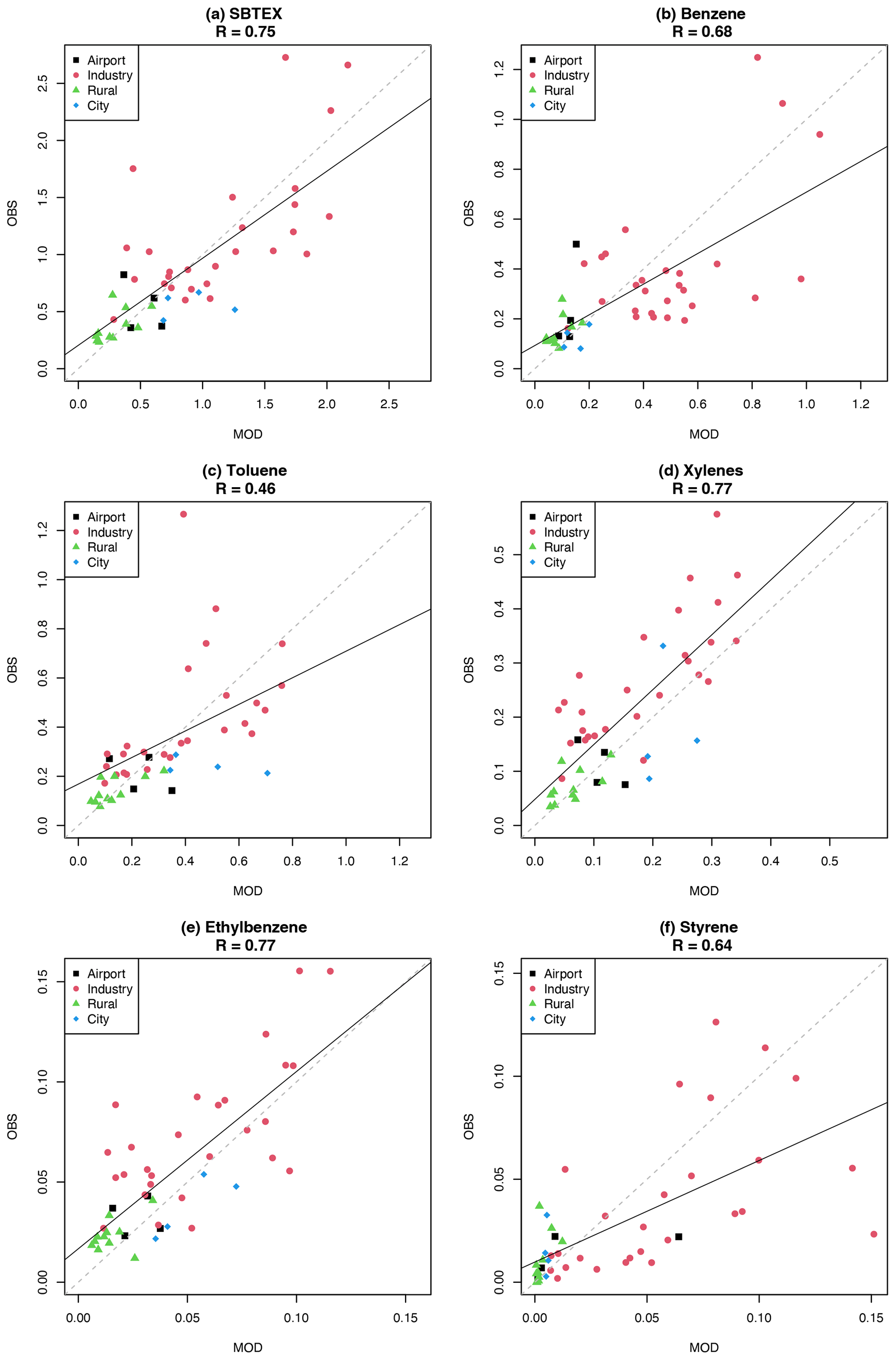
Figure 6 The average SBTEX concentration (ppb) comparison between the model (MOD) Adj case and observational (OBS) data during the model simulation period (1 May to 30 September 2012) for (a) total SBTEX, (b) benzene, (c) toluene, (d) xylenes, (e) ethylbenzene, and (f) styrene.

We further classified the observation sites into four groups, including “Airport”, “Industry”, “Rural”, and “Urban”, based on their geographical locations (Table S8). For the total SBTEX (Fig. 6a), the correlation coefficient (R) is 0.75 (R² is 0.56) across all the locations, and the black solid line is the regression line for all the sites (N=46). The red dots indicated that the industrial sites have a higher concentration in both the model and observational results, and the cities (blue diamonds) showed that their concentrations are slightly overestimated and lower than the industrial sites. Airport (black squares) and Rural (green triangles) have lower SBTEX concentrations than City and Industry, and Rural is the lowest group. Figure 6b to f are similar plots for explicit benzene, toluene, xylenes, ethylbenzene, and styrene. R ranges from 0.46 to 0.77. Benzene (R is 0.68), toluene (R is 0.46), and styrene (R is 0.64) are overestimated, but xylenes (R is 0.77) and ethylbenzene (R is 0.77) are close to the observational data. Although toluene has the lowest R (0.46), this is caused by two industry sites that largely underestimate in Houston (site ID: 482011015) and Nederland (site ID: 482450014). In case we remove these two industrial sites' data, the R for toluene in Fig. 6c will become 0.7 (Fig. S7). This phenomenon is probably caused by the missing toluene industrial sources near those two sites. The inclusion of missing emission sources definitively improved the model performance (Table 2), especially in the Rural (+5.4 %) and Airport groups (+6.8 %), which suffered the most due to the missing industrial sources. The NMBs for xylenes are also reduced across all the emission groups (Industry: +3 %, Urban: +12 %, Airport: +20 %, and Rural: +13 %).

Because only a few sites have hourly data, this study compared the diurnal variation of SBTEX concentrations for the Houston industrial area (using data from only three monitoring sites) in Fig. S8. The hourly data show that benzene, ethylbenzene, and styrene are overestimated (the NMB for benzene is 69 %, ethylbenzene is 36 %, and styrene is 27 %) during nighttime hours (21:00 to 06:00 LT). Toluene is underestimated at nighttime (the NMB is −45 %), whereas xylenes closely align with the observed data (−16 %) range. On the other hand, all species experience underestimation during daytime hours (the NMB for benzene is −25 %, toluene is −65 %, xylenes are −51 %, ethylbenzene is −46 %, and styrene is −82 %) (from 10:00 to 17:00 LT). Such results indicate that the hourly emission rate may overestimate during nighttime but underestimate during daytime in the Houston industrial area.

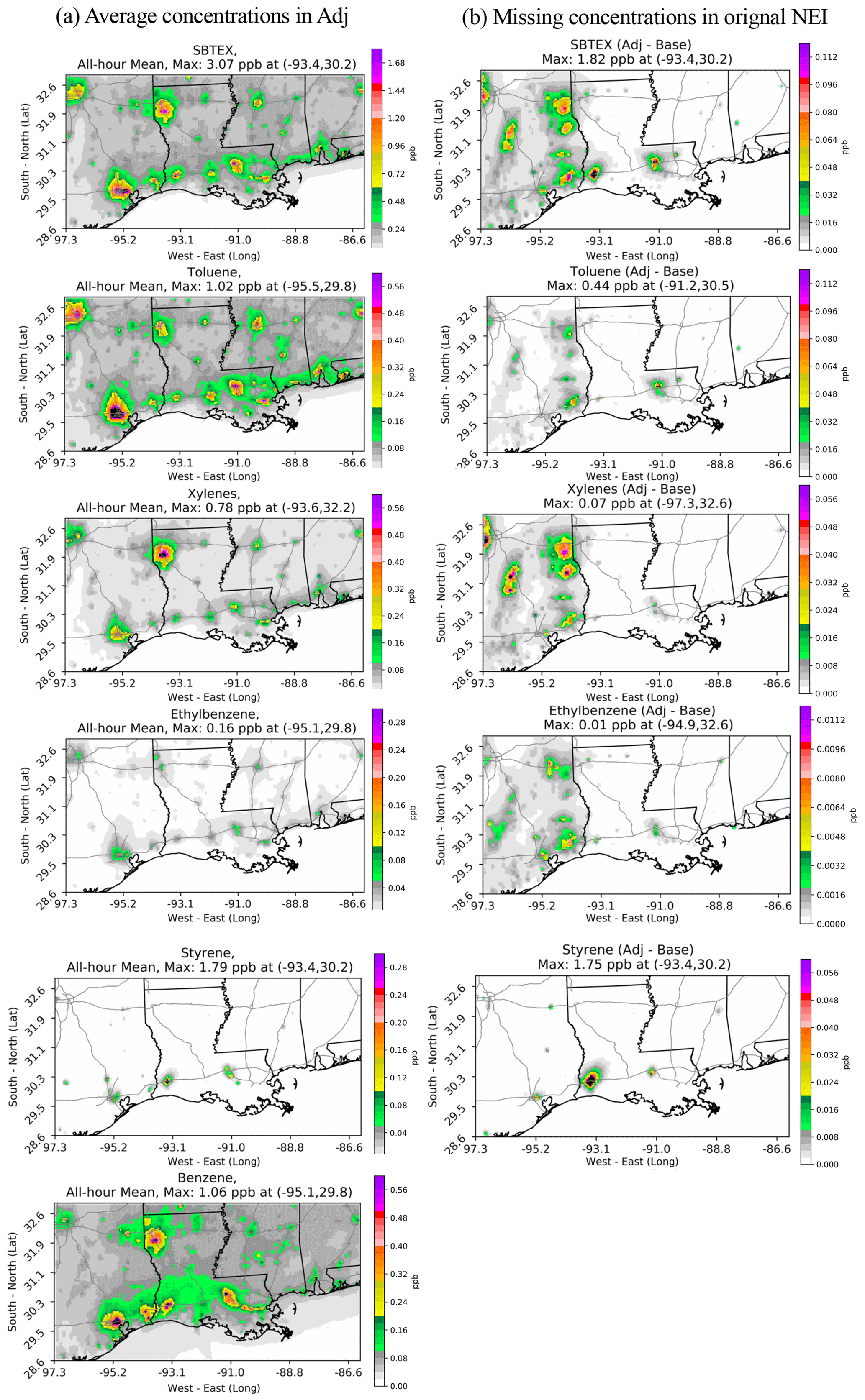
Figure 7 The average concentration (a) and missing concentration (b) of SBTEX during the model simulation period (1 May to 30 September 2012) in the Adj scenario. The black color indicates that the concentration is higher than the maximum color-scale bar.

3.3 SBTEX concentration patterns

3.3.1 Spatial distribution

Figure 7a presents the spatial distribution of SBTEX concentrations during the model period (1 May to 30 September) in the Adj scenario. The highest SBTEX concentration (3.07 ppb) occurs near Lake Charles, followed by Baton Rouge (2.06 ppb), the Houston ship channel (2.04 ppb), Shreveport (1.69 ppb), and Beaumont (1.59 ppb). The spatial distribution patterns of the individual SBTEX compounds exhibit similarities due to the shared emission sources, except for styrene. Styrene primarily originates from ptnonipm, while the other species predominantly arise from vehicle emissions and wildfires. Benzene (maximum 1.06 ppb), toluene (maximum 1.01 ppb), and ethylbenzene (maximum 0.16 ppb) reach their highest concentrations in Houston, reflecting their significant emissions. Further, xylenes (0.78 ppb) originate from the sources in Shreveport. Remarkably, elevated concentrations of styrene (reaching 1.97 ppb) are conspicuously identified as being proximal to Lake Charles, a locale characterized by an abundant emission of styrene from non-electricity-generating unit point sources, which were absent in the original NEI records.

This study further investigated the influence of missing emission sources in the original NEI on the SBTEX concentrations by taking the differences between the Adj and Base scenarios. The majority of the missing emissions are associated with the np_oilgas and ptnonipm sectors, with increased contributions geographically concentrated in Texas and Louisiana (Fig. 7b). In particular, the largest impact on the SBTEX concentrations is shown near Lake Charles by up to 1.82 ppb (+68 %), which is mostly related to the increase in the styrene concentration (by 1.75 ppb, +5315 %). This increase is due to the NEI missing one large point source (364.12 t yr⁻¹) in the ptnonipm sector near Lake Charles. The inclusion of the missing emission sources also led to the increase in styrene concentrations in other cities, such as Baton Rouge (0.07 ppb, +389 %), LA, and Houston, TX (0.03 ppb, +62 %). Baton Rouge, LA, also suffers the highest increase in toluene concentrations by 0.44 ppb (+92 %) due to the inclusion of missing emissions, followed by Beaumont (0.07 ppb, +50 %) and Carthage (0.048 ppb, +66 %), TX. Fort Worth, TX, exhibits the highest increase in xylene concentrations by 0.07 ppb (+95 %), followed by Center (0.06 ppb, +273 %), Teague (0.06 ppb, +340 %), and Beaumont (0.036 ppb, +70 %), TX. The largest increase in the ethylbenzene concentration occurred at Longview (0.01 ppb, +85 %), followed by Beaumont (0.009 ppb, +40 %) and Houston (0.006 ppb, +9 %), TX.

3.3.2 The diurnal variation

In general, the diurnal variations of SBTEX concentrations are primarily influenced by various factors (such as ventilation, emissions, diffusion, deposition, and chemical reactions). These variations typically manifest with lower concentrations during the daytime compared to the nighttime due to increased ventilation, diffusion, and chemical loss, even though the emissions are about 4 times higher during the daytime, as presented earlier (Fig. 4). Diurnal meteorological and emission patterns suggest more sensitivity of the concentrations to the emissions during nighttime than daytime, implying that implementing emission controls to reduce the concentrations at night would be most effective. The variation of emission sources might also modulate the diurnal pattern in the concentrations. To demonstrate this, here we selected two industrial locations and one city location with high SBTEX concentrations to compare the diurnal variation of the concentrations.

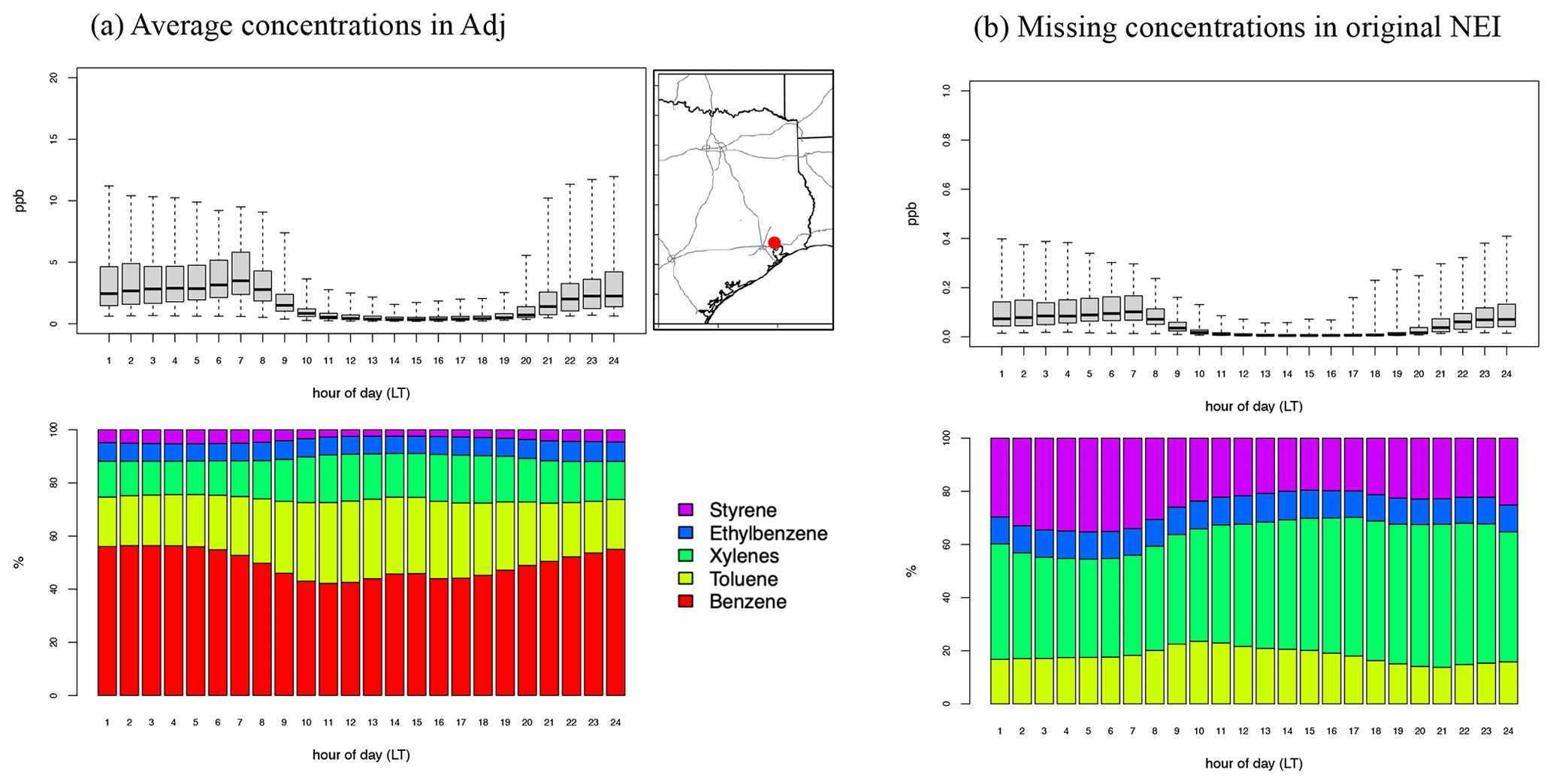
Figure 8 Diurnal pattern (upper panel) and relative composition (lower panel) of SBTEX concentrations (a) and the missing concentration (b) from 1 May to 30 September in the Houston Ship Channel industry area, Channelview city (red dot location).

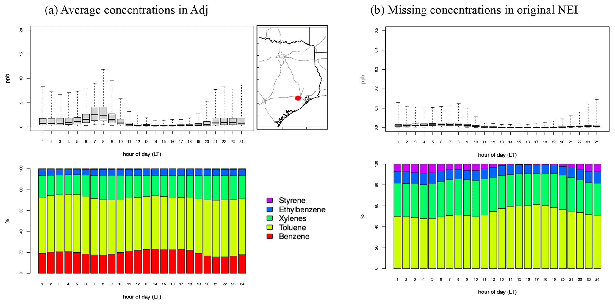
Figure 9 Diurnal pattern (upper panel) and relative composition (lower panel) of SBTEX concentrations (a) and missing concentrations (b) from 1 May to 30 September in the Houston residential area near Bayland Park (red dot location).

The first one is Channelview city (latitude 29.8, longitude −95.12), located in the Houston ship channel industrial area on the eastern side of downtown Houston. Driven by both emission temporal profiles and meteorological conditions, the peak SBTEX concentration (about 12 ppb) in Channelview city occurs at 23:00 to 01:00 LT, contributed mostly by benzene (56 %), which indicates industrial sources with small amounts of toluene (19 %), xylenes (13 %), styrene (4.8 %), and ethylbenzene (7 %) (Fig. 8a). The second case, Bayland Park (latitude 29.69, longitude −95.49), located nearby on the western side of Houston, presents the same level of the peak SBTEX concentration (about 12 ppb) (Fig. 9a) as Channelview city. In contrast to Channelview city, the peak concentration of Bayland Park occurs at the traffic rush hour (07:00 to 08:00 LT), contributed mostly by toluene (53 %) and xylenes (23 %) (indicating mobile vehicle sources) rather than benzene (18 %). Meanwhile, the adjusted industry emission sources, as presented in Table S5, play a significant role in driving the peak concentration (0.4 ppb) in Channelview city (Fig. 8b) yet exhibit a reduced impact on Bayland Park (Fig. 9b), which is far from the industry area.

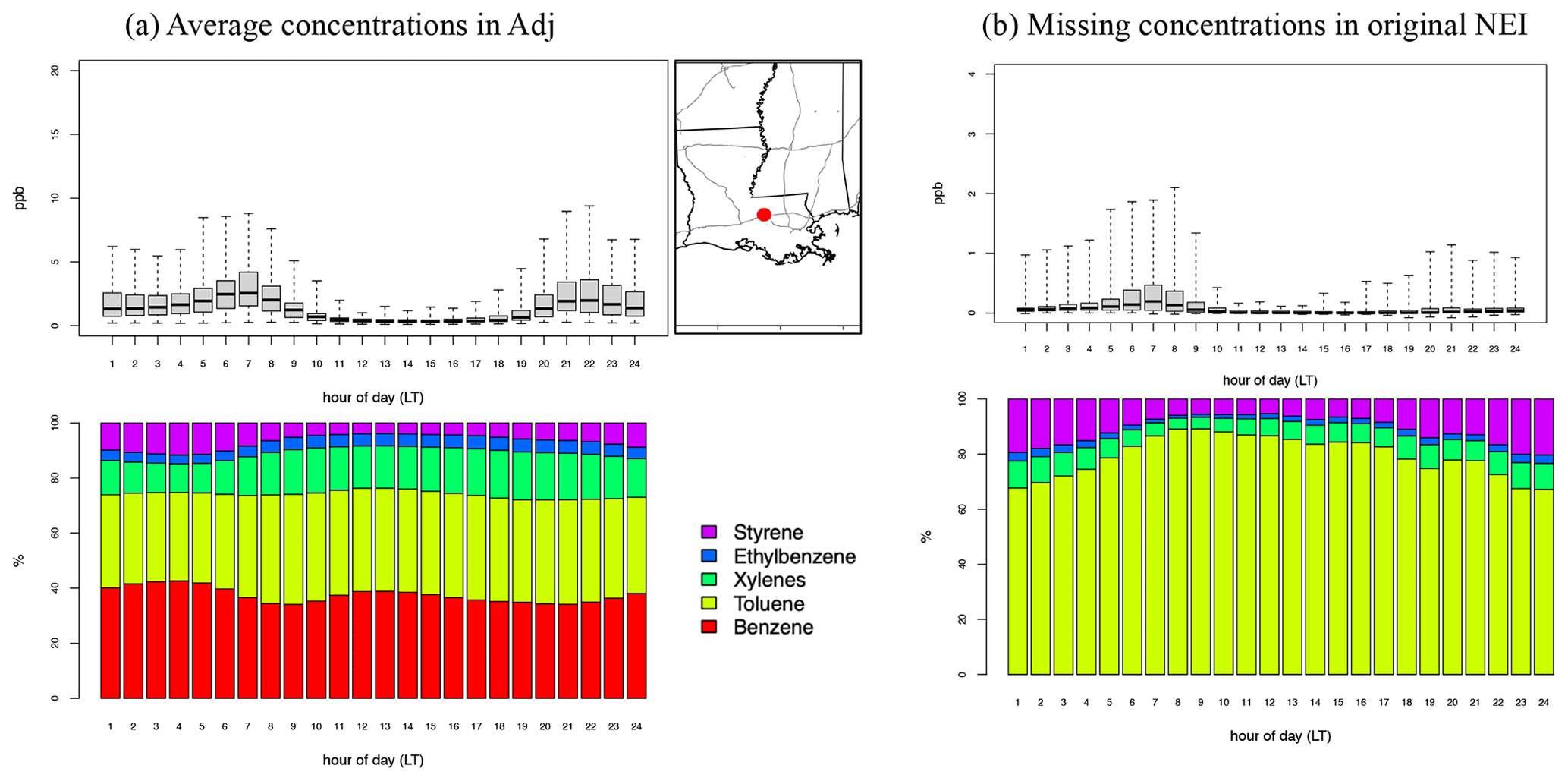
Figure 10 Diurnal pattern (upper panel) and relative composition (lower panel) of the SBTEX concentrations (a) and missing concentration (b) from 1 May to 30 September in Baton Rouge (red dot location).

A similar pattern is also shown in Baton Rouge, Louisiana (latitude 30.46, longitude −91.17), located near downtown Baton Rouge (affected by on-road sources) and also close to the industry area (∼1.6 km from the north). Like the Houston industry area, the daytime SBTEX concentration is much lower (<3 ppb) than nighttime, and the peak SBTEX concentration (about 9.4 ppb) occurs at 22:00 LT (Fig. 10). Because Baton Rouge is impacted by both traffic and industrial sources, emissions differ from Houston in that both benzene (35 %–40 %) and toluene (35 %–40 %) become the major portion of SBTEX (Fig. 10a). The missing emission sources (Fig. 10b) will further enhance the peak concentration by 2 ppb at 05:00–08:00 LT, with the largest chemical contribution from toluene (about 70 %–85 %), followed by the styrene (about 7 %–20 %) associated with the industrial sources.

4 Data availability

1. The results of this study, including the SBTEX emission, concentration data and evaluation code, can be downloaded at https://doi.org/10.5281/zenodo.7967541 (Wang et al., 2023).

2. Besides May to September 2019, we also provided the whole 2012 SBTEX hourly concentration data of the Adj case in NetCDF format and “comma-separated values (csv)”.

3. The 2011 NEI emission model platform (EMP) and the SMOKE model system can be downloaded on the EPA ftp website: https://www.epa.gov/air-emissions-modeling/2011-version-6-air-emissions-modeling-platforms (USEPA, 2021b).

4. The meteorological data can be found on the CMAS Data Warehouse website: https://dataverse.unc.edu/dataverse/cmascenter (UNC-IE, 2021).

5. The AMTIC data can be found at https://www.epa.gov/amtic/amtic-ambient-monitoring-archive-haps (USEPA, 2021c).

5 Code availability

1. The source code of the CAMx7.00 model and the model preprocess tools (O3map, tuv4.8, wrfcamx, camq2camx) can be downloaded on the Environ website: http://www.camx.com (Ramboll, 2021).

2. Python 2.7 is used to treat the model output and can be downloaded on the Anaconda Python website: https://www.anaconda.com/products/individual (Anaconda, 2020).

3. The R project for statistical computing can be downloaded at https://www.r-project.org (The R Foundation, 2021).

4. HAPI program code can be downloaded on GitHub: https://github.com/tatawang/HAPI (last access: 25 November 2023), https://doi.org/10.5281/zenodo.7987106 (Wang and Baek, 2023).

6 Conclusion and discussion

To address the urgent need for health assessment of SBTEX exposures in the Gulf region, this study developed high spatiotemporally resolved emissions and concentrations of the individual SBTEX. The HAPI program was developed and implemented to identify and gap-fill the missing SBTEX inventory for the SMOKE emission modeling system. Then, the state-of-the-science chemical transport modeling system, CAMx, was applied to generate the high temporal and spatial resolution predictions of explicit SBTEX concentrations based on the improved SBTEX emission inventory and the Reactive Tracer (RTRAC) feature. The modeled average SBTEX concentrations exhibit good agreement with observational data (R is 0.75 and NMB is improved in the Adj case to −5.6 % for the total SBTEX), suggesting that the emissions and concentration estimates developed in this study can be used to support well the SBTEX-related human health studies in the Gulf region.

This study found that the on-road sector contributes the most to the total xylenes (46 %), toluene (48 %), and ethylbenzene (60 %) emissions, while the styrene emissions are mostly contributed by non-EGU point sources (ptnonipm, 69 %) but were substantially underestimated in the original NEI data, resulting in 34 % underestimation of total styrene emissions. The highest SBTEX concentration (3.07 ppb) occurs near Lake Charles, followed by Baton Rouge (2.06 ppb), Houston ship channel (2.04 ppb), Shreveport (1.69 ppb), Beaumont (1.59 ppb), corresponding to a large amount of SBTEX emissions in these cities.

The 5-month average SBTEX modeled concentrations are close to the average measurement data (R of total SBTEX is 0.74, benzene is 0.68, toluene is 0.45, xylenes is 0.77, ethylbenzene is 0.77, and styrene is 0.64). These spatiotemporally fine modeled air SBTEX concentrations can be used for conducting epidemiologic analyses or in risk assessment. The diurnal variation of SBTEX concentrations that is opposite to its emissions pattern indicates that the concentration is more sensitive to emission at night than daytime. The high SBTEX concentration during nighttime affects individuals who engage in more nighttime activities or reside in houses lacking isolation of outdoor air. Therefore, the HAP emission control policy should also focus on nighttime emissions. Further, the hourly SBTEX data can be used in epidemiologic analyses to investigate effects of acute exposures and short-term changes in those exposures.

This study acknowledges the considerable uncertainties in this approach, including the accuracy of emission data, the meteorological condition data, oxidant concentrations (OH radical, O₃, and NO₃) simulation in the CB6 mechanism. There are limited observational data to verify the model performance. This study is mainly based on the bottom-up NEI dataset, thus the uncertainties in the original NEI emissions and SMOKE process influenced on this study. For example, despite our implementation of imputation for the HAP annual data, the emission activity within hourly, daily, and monthly temporal profiles as well as parameters (e.g., emission rates, and compositions) also remains unchanged. The emergency emissions from unreported flaring (such as final treatment equipment) or leakage events that have not been considered in the original NEI, also not included in this study. Further, the concentrations of oxidants are simulated in the CAMx model with the CB6r4 mechanism; this mechanism is designed to simulate ozone and PM. Therefore, the model species OH radical, NO₃, and O₃ may differ from the actual concentrations. These oxidant concentrations affect the chemical decay rate, especially in big metropolitan cities with higher NO_x emissions. Nevertheless, the high spatiotemporally resolved emissions and concentrations of individual SBTEX developed in this study, with acceptable performance, can be a good reference dataset to support SBTEX-related human health studies in the Gulf region. In addition, this approach can be extended to other chemical compounds to estimate their concentrations. The US EPA provides emission data for approximately 100 HAPs in the NEI for certain emission sources. Those emission data can also be processed to derive HAP concentrations. The dataset provided in this study will facilitate epidemiologic studies of SBTEX exposures in relation to a range of health outcomes in the Gulf region and can be extended to provide similar health research opportunities elsewhere.