Quality-controlled meteorological datasets from SIGMA automatic weather stations in northwest Greenland, 2012–2020

In situ meteorological data are essential to better understand ongoing environmental changes in the Arctic. Here, we present a dataset of quality-controlled meteorological observations from two automatic weather stations in northwest Greenland from July 2012 to the end of August 2020. The stations were installed in the accumulation area on the Greenland Ice Sheet (SIGMA-A site, 1490 m a.s.l.) and near the equilibrium line of the Qaanaaq Ice Cap (SIGMA-B site, 944 m a.s.l.). We describe the two-step sequence of quality-controlling procedures that we used to create increasingly reliable datasets by masking erroneous data records. Those datasets are archived in the Arctic Data archive System (ADS) (SIGMA-A – https://doi.org/10.17592/001.2022041303, Nishimura et al., 2023f; SIGMA-B – https://doi.org/10.17592/001.2022041306, Nishimura et al., 2023c). We analyzed the resulting 2012–2020 time series of air temperature, surface height, and surface albedo and histograms of longwave radiation (a proxy of cloudiness). We found that surface height increased, and no significant albedo decline in summer was observed at the SIGMA-A site. In contrast, high air temperatures and frequent clear-sky conditions in the summers of 2015, 2019, and 2020 at the SIGMA-B site caused significant albedo and surface lowering. Therefore, it appears that these weather condition differences led to the apparent surface height decrease at the SIGMA-B site but not at the SIGMA-A site. We anticipate that this quality-controlling method and these datasets will aid in climate studies of northwest Greenland and will contribute to the advancement of broader polar climate studies.

1 Introduction

Automatic weather observations in Greenland started with GC-Net (Greenland Climate Network; Steffen and Box, 2001), which was established as a network of automatic weather stations (AWSs) in Greenland after 1990. This observation network was intended to provide long-term observations of climatological and glaciological factors over Greenland. This was followed by the deployment of PROMICE (van As et al., 2011; Fausto et al., 2021), led by the Geological Survey of Denmark and Greenland (GEUS), and the K-transect network (van de Wal et al., 2005), led by Utrecht University in the Netherlands. PROMICE is currently operating the largest observation network in Greenland by contracting the maintenance of GC-Net equipment, and K-transect has deployed equipment mainly in the western part of the country and continues to monitor the area closely. Both networks have provided important long-term meteorological data.

To contribute to these efforts and to fill a spatial gap, we established two AWS systems in northwest Greenland (Fig. 1), where rapid environmental changes have occurred in recent years (Aoki et al., 2014). Recent studies of this region have documented a drastic mass loss since the mid-2000s (Mouginot et al., 2019), an expansion of the ablation area (Noël et al., 2019), and a hotspot of increasing rainfall (Niwano et al., 2021). The two sites were established in 2012 as a part of the Snow Impurity and Glacial Microbe effects on abrupt warming in the Arctic (SIGMA) project, which aimed to clarify the dramatic enhancement of the melting of the Greenland Ice Sheet induced by snow impurities (e.g., black carbon, mineral dust). The observational data acquired since that time have been used by glaciological (Yamaguchi et al., 2014; Tsutaki et al., 2017; Matoba et al., 2018; Kurosaki et al., 2020), meteorological (Aoki et al., 2014; Tanikawa et al., 2014; Niwano et al., 2015; Hirose et al., 2021), and biological studies (Onuma et al., 2018; Takeuchi et al., 2018). These data are also valuable because they support the evaluation and development of numerical models (e.g., Niwano et al., 2018; Fujita et al., 2021).

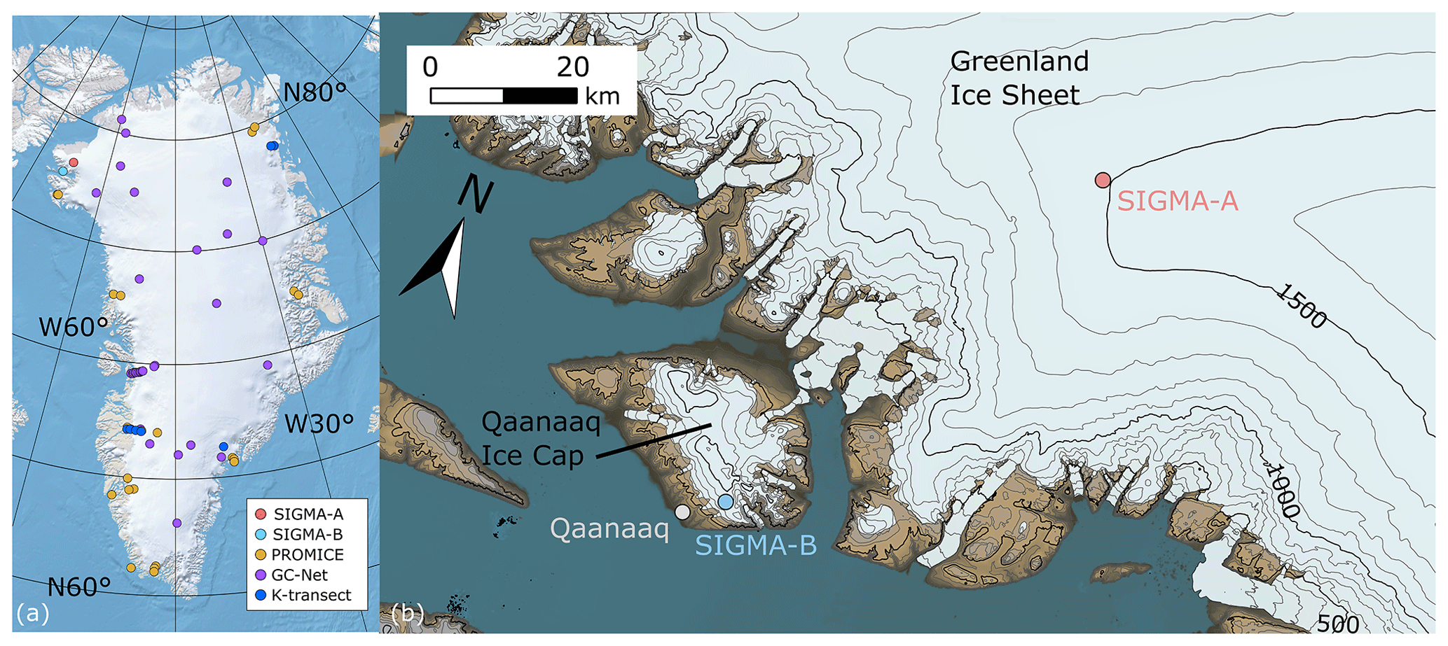
Figure 1 (a) Location map of Greenland showing PROMICE, GC-Net, and K-transect AWS sites and (b) a local map of northwest Greenland showing locations of AWS sites SIGMA-A and SIGMA-B. Contour interval in (b) is 100 m.

The datasets from AWSs generally contain erroneous data records that are attributed to natural factors (e.g., riming, ice accretion, snow accumulation on sensors) or technical issues (e.g., zero offset – Behrens, 2021; faulty sensors) for radiation sensors. Various procedures exist for improving the quality of such datasets (e.g., Fiebrich et al., 2010; Fausto et al., 2021). In particular, careful quality control (QC) procedures, which constitute a process to improve the quality of data by removing outliers, are required for downward radiation sensors, which are sensitive to solar zenith angle, icing, riming, and snowfall (van den Broeke et al., 2004a, b; Moradi, 2009). Other QC procedures deal with error sources through range, step, and internal consistency tests (Estévez et al., 2011). The specifics of QC methods, for example, the threshold value for detecting erroneous data records, should be adjusted for each observation environment. In this paper, we describe the QC methods used for the in situ meteorological observation data from northwest Greenland, which include existing QC methods, new ones, and combinations of both.

After describing the AWS sites (Sect. 2) and their datasets (Sect. 3), this paper introduces the two separate QC methods used sequentially to mask erroneous data records (Sect. 4). We then present examples of time series of meteorological variables in northwest Greenland, infer their implications for interannual variations in weather conditions, and describe the differences between the two sites (Sect. 5).

2 AWS general description

The two AWSs are installed at the SIGMA-A site (78.052^∘ N, 67.628^∘ W; 1490 m a.s.l.) on the northwest Greenland Ice Sheet and the SIGMA-B site (77.518^∘ N, 69.062^∘ W; 944 m a.s.l.) on the Qaanaaq Ice Cap, a peripheral ice cap on the Greenland coast (Fig. 1). They have been in operation since July 2012 (Aoki et al., 2014). The observed parameters and the sensor specifications, including abbreviations, are listed in Table 1. The other key constants and variables (and their abbreviations) used in this study are also in Table 2.

Table 1 Meteorological observation parameters and sensor specifications.

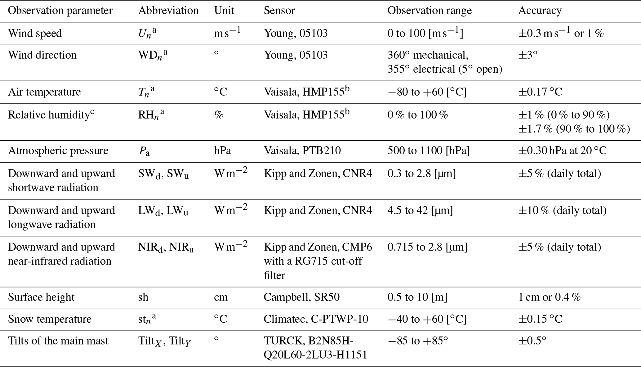
^a The n suffix is appended to distinguish the observation height or depth. ^b Protected from direct solar irradiance by a naturally aspirated 14-plate Gill radiation shield. ^c Relative humidity is measured relative to water even in sub-freezing environments.

Table 2 Key constants, variables, and their symbols used in this paper.

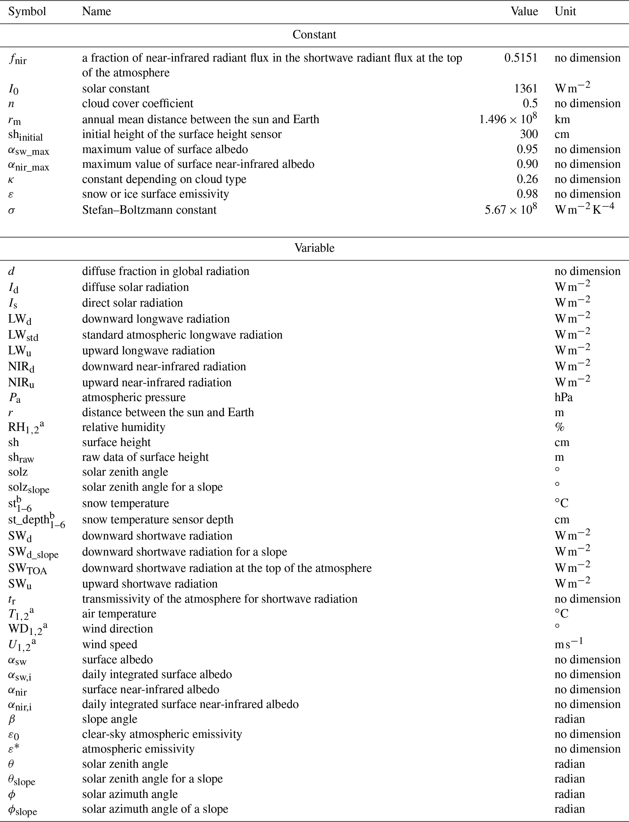
^a 1: Observed at lower height, 2: observed at upper height (only at the SIGMA-A site). ^b 1–6: Observing depth.

The SIGMA-A site is 70 km inland from the coast on a ridge of the Greenland Ice Sheet extending northwest from the Greenland Summit; it sits on a flat snow surface with no obstacles around the site (see Fig. 2). This site is in an accumulation area of the ice sheet (Matoba et al., 2018) based on the analysis of ice core data (Yamaguchi et al., 2014; Matoba et al., 2017). The SIGMA-B site is 3 km north of the village of Qaanaaq. This site is considered to be located near the equilibrium line (910 m a.s.l.; Tsutaki et al., 2017) on the Qaanaaq Ice Cap, which ranges in elevation between 30 and 1110 m a.s.l. (Sugiyama et al., 2014). The surface condition at this site varies (see Fig. 2), and significant surface lowering has occurred in warm years (e.g., Aoki et al., 2014). The site is located on a southwest-facing slope (azimuth 220^∘) with an angle of 4^∘ according to 10 m DEM data (Porter et al., 2018).

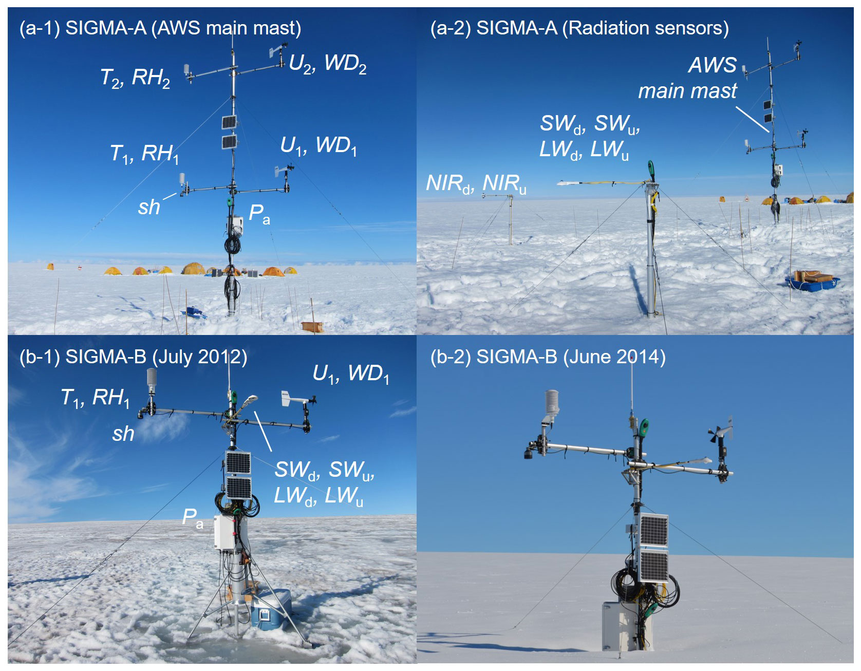
Figure 2 Setting and instrumentation at the SIGMA-A site (a-1, a-2) and the SIGMA-B site (b-1, b-2). Surface conditions at SIGMA-B are shown for July 2012 and June 2014. Sensors are labeled with the observation parameters they measure (see Table 1).

3 Description of AWS systems and datasets

3.1 Specifications

Each AWS main mast is set in a hole drilled using a hand auger. Sensors for air temperature, relative humidity, and wind speed and direction are mounted at the ends of horizontal poles to exclude possible thermal and wind disturbances from the main mast. The SIGMA-A sensors are placed 3 and 6 m above the surface, as signified by subscripts 1 (lower) and 2 (upper) in the corresponding data variables. The SIGMA-B sensors are set at 3 m above the surface and have subscripts of 1. The surface height sensor at both sites is mounted at 3 m height beneath the air temperature and relative humidity sensors. Six snow temperature sensors have been set as follows. Four sensors were set at 19:00 UTC on 29 June 2012 at depths of 100 cm (st₁), 70 cm (st₂), 40 cm (st₃), and 5 cm (st₄) below the snow surface. At 21:00 UTC on 27 July 2013, sensors st₃ and st₄ were relocated to depths of 46 and 16 cm, respectively. Sensors st₅ and st₆ were set at 5 cm under the surface and 45 cm above the surface, respectively, at 14:00 UTC on 9 June 2014. Sensors for shortwave, longwave, and near-infrared radiation were installed at SIGMA-A on separate poles 10 m from the main mast (Fig. 2a-2). A pyranometer and a pyrgeometer at SIGMA-B were mounted on the main mast facing directly south. Tilt angles of the main mast in the north–south (Tilt_X) and east–west (Tilt_Y) directions were monitored with an inclinometer attached to the main mast. The additional suffixes A or B represent the site name in the variables introduced below.

Electric power is supplied to the AWS systems by a lead-acid battery that is charged constantly by solar panels attached to the main mast. All parameters are recorded once per minute and stored in a data logger (C-CR1000, Campbell Scientific, USA), except for the main mast's surface height and tilt angles, which are recorded every hour. Hourly data are calculated for the other parameters by averaging the 1 min data. All hourly data are sent regularly to the data server via the Argos satellite channel.

Surface height is measured with an ultrasonic snow gauge (Table 1). The raw data from this sensor (sh_raw) are the distance from the sensor to the snow surface, which has a temperature dependence. The temperature-corrected surface height (sh) is calculated from

$$\begin{array}{}\text{(1)}& \text{sh}={\text{sh}}_{\text{initial}}-{\text{sh}}_{\text{raw}}\times \sqrt{{\displaystyle \frac{T_{\mathrm{2}}+\mathrm{273.15}}{\mathrm{273.15}}}}\times \mathrm{100},\end{array}$$

where sh_initial (=300 cm) is the initially installed sensor height from the surface, and T₂ is air temperature.

3.2 Data processing

We describe the calculations for some variables used in the QC process in this section. To accurately calculate the surface albedo and surface energy balance at the SIGMA-B site, we considered the impact of the sloping surface on the vertical radiant flux. To account for this effect, we derived the slope-corrected downward shortwave radiation (SW_{d_slope}) using the methods in Jonsell et al. (2003) and Hock and Holmgren (2005). The SW_{d_slope} is calculated by

$$\begin{array}{}\text{(2)}& {\text{SW}}_{\text{d\_slope}}=I_{\mathrm{s}}+I_{\mathrm{d}},\end{array}$$

where I_s and I_d are the direct and diffuse shortwave radiation for a slope, respectively:

$$\begin{array}{}\text{(3)}& {\displaystyle }{I}_{\mathrm{s}}& {\displaystyle }={\text{SW}}_{\mathrm{d}}\times d,\text{(4)}& {\displaystyle }{I}_{\mathrm{d}}& {\displaystyle }={\text{SW}}_{\mathrm{d}}\times (\mathrm{1}-d)\times {\displaystyle \frac{\cos {\mathit{\theta }}_{\text{slope}}}{\cos \mathit{\theta }}},\end{array}$$

where d is the ratio of total diffuse radiation to global radiation, and θ and θ_slope [radian] are the solar zenith angle and the solar zenith angle for a slope, respectively. The ratio d is obtained from atmospheric transmittance t_r by

$$\begin{array}{}\text{(5)}& d=\left\{\begin{array}{ll}\mathrm{0.15}& \mathrm{\text{for }}\mathrm{0.8}\le t_{\mathrm{r}},\\ \mathrm{0.929}+\mathrm{1.134}{t}_{\mathrm{r}}-\mathrm{5.111}{t}_{\mathrm{r}}^{\mathrm{2}}+\mathrm{3.106}{t}_{\mathrm{r}}^{\mathrm{3}}& \\ & \mathrm{\text{for }}\mathrm{0.15}<t_{\mathrm{r}}<\mathrm{0.8},\\ \mathrm{1.0}& \mathrm{\text{for }}{t}_{\mathrm{r}}\le \mathrm{0.15},\end{array}\right.\end{array}$$

where

$$\begin{array}{}\text{(6)}& t_{\mathrm{r}}={\displaystyle \frac{{\text{SW}}_{\mathrm{d}}}{{\text{SW}}_{\text{TOA}}}},\end{array}$$

where SW_TOA is the downward shortwave radiation at the top of the atmosphere, calculated by

$$\begin{array}{}\text{(7)}& {\text{SW}}_{\text{TOA}}=I_{\mathrm{0}}{\left({\displaystyle \frac{r_{\mathrm{m}}}{r}}\right)}^{\mathrm{2}}\cos \mathit{\theta },\end{array}$$

where I₀ (=1361 W m⁻²) is the solar constant (Rottman, 2006; Fröhlich, 2012), r is the distance between the sun and Earth (assuming an elliptical orbit with an eccentricity of 0.01637), and r_m is its annual mean ($=\mathrm{1.496}\times {\mathrm{10}}^{\mathrm{8}}$ km).

The solar zenith angle for a slope in Eq. (4) is calculated by

$$\begin{array}{}\text{(8)}& \cos {\mathit{\theta }}_{\text{slope}}=\cos \mathit{\beta }\cos \mathit{\theta }+\sin \mathit{\beta }\sin \mathit{\theta }\cos (\mathit{\phi }-{\mathit{\phi }}_{\text{slope}}),\end{array}$$

where β is the slope angle from a horizontal plane, and φ and φ_slope are the solar azimuth and the solar azimuth for the slope direction, respectively. Solar zenith and azimuth angles are calculated from the geographic position of the observation site and the date and time.

Shortwave and near-infrared albedos (a_sw and a_nir, respectively) are calculated as the ratio of upward and downward radiant fluxes, as shown for a_sw by

$$\begin{array}{}\text{(9)}& {\mathit{\alpha }}_{\text{sw}}={\displaystyle \frac{{\text{SW}}_{\mathrm{u}}}{{\text{SW}}_{\mathrm{d}}}},\end{array}$$

where SW_u is the upward shortwave radiant flux and SW_d is the downward shortwave radiant flux. SW_{d_slope} is used for SW_d when calculating a_sw at the SIGMA-B site. The daily integrated shortwave albedo (a_sw,i) is calculated as the ratio of cumulative upward and downward radiant fluxes for the past 24 h:

$$\begin{array}{}\text{(10)}& {\mathit{\alpha }}_{\text{sw,i}}=\sum _{\text{24\hspace{0.17em}h}}{\text{SW}}_{\mathrm{u}}/\sum _{\text{24\hspace{0.17em}h}}{\text{SW}}_{\mathrm{d}}.\end{array}$$

The near-infrared albedo (a_nir) and daily integrated near-infrared albedo (a_nir,i) are calculated in the same way. The near-infrared fraction is the ratio of the downward near-infrared radiant flux (NIR_d) to SW_d.

Note that some parameters may require correction or caution depending on the observation environment. First, since temperature and humidity shelters are naturally ventilated, air temperature value may have a positive bias due to shelter heating from solar radiation (e.g., Morino et al., 2021). In addition, in sub-freezing conditions, relative humidity may not be measured correctly because the sensor used in this study (Vaisala, HMP155) calculates relative humidity as liquid water vapor pressure even in sub-freezing environments and even when the shelter is covered by rime or frost (Makkonen and Laakso, 2005). Aoki et al. (2011) pointed out that the pole on which the radiometer is mounted casts a shadow on the radiation sensor. In addition, reflection and shielding of scattered radiation due to the AWS including solar panels may result in incorrect radiation measurements, although no anomalous radiation data due to these factors were found. Although the possibility of data correction as described above is recognized, the focus of this paper is to open the observed values themselves without any correction or data processing that might involve the implementer's intention. Therefore, we will note only the correction possibilities and present the observed data in this study.

4 Quality control

The datasets of observations at sites SIGMA-A and SIGMA-B are classified into four QC levels numbered 1.0 to 1.3. A level-1.0 dataset, which is not archived in any repository, is a raw dataset without data processing. A level-1.1 dataset is a raw dataset with flags added to indicate missing data for periods when the data logger was inoperative. A level-1.2 dataset has undergone an initial control, which uses a simple masking algorithm to eliminate anomalous values that violate physical laws or that are impossible in the observed environment. The initial control improves the accuracy of the statistical processing that follows and reduces the possibility of excluding true values. A level-1.3 dataset has undergone a secondary control in which statistical methods are used on level-1.2 data to identify and mask outlier values. It has also undergone a final manual masking procedure, in which a researcher visually checks the dataset and masks outliers based on subjective criteria.

The initial control method is described in Sect. 4.1, and the secondary control method is described in Sect. 4.2. In these sections, the parameter suffixes related to the differences in observation height (1 and 2) and site (A and B) are omitted except when needed for clarity, and subscripts indicating upward and downward radiation (d – downward, u – upward) are denoted as χ in the equation. Erroneous records are flagged with one of the following numerical expressions to signify the reason they have been flagged:

• The expression −9999 indicates a missing or erroneous data record attributed to a mechanical malfunction or a local phenomenon such as sensor icing, riming, or burial in snow.

• The expression −9998 indicates an erroneous radiation record when the radiant sensor was covered with snow or frost.

• The expression −9997 indicates a record of snow temperature sensor depth when the sensor was suspected to be located above and not below the snow surface.

• The expression −8888 indicates a record flagged during the manual masking procedure.

4.1 Initial QC for level-1.2 datasets

The objectives of the initial control are to eliminate erroneous records due to mechanical malfunctions or local phenomena and to pre-treat level-1.1 datasets for the secondary control. The initial control consists of a range test (e.g., Fiebrich et al., 2010; Estévez et al., 2011) and a manual masking procedure. The range test sets variation ranges (see Tables 3 and 4) for each observed parameter in northwest Greenland on the basis of simple statistics based on maximum, minimum, and mean values derived from records in the level-1.1 dataset during a period with no obvious erroneous data. Records outside this statistical range are flagged with a −9999 code. Tables 3 and 4 list the parameters subjected to this test and their assigned ranges. The manual masking procedure identified specific erroneous values that resulted from an electrical malfunction and flagged them with a −8888 code. The following subsections offer detailed and additional explanations of the initial control; however, the range test for each parameter is listed in Table 3. Detailed descriptions of each parameter are omitted in the following sections.

Table 3 Range test coverage for each parameter used in the QC procedures. The variable subscripts n (1 or 2) and χ indicate the distinction of sensor height and the direction of radiation flux (upward or downward), respectively.

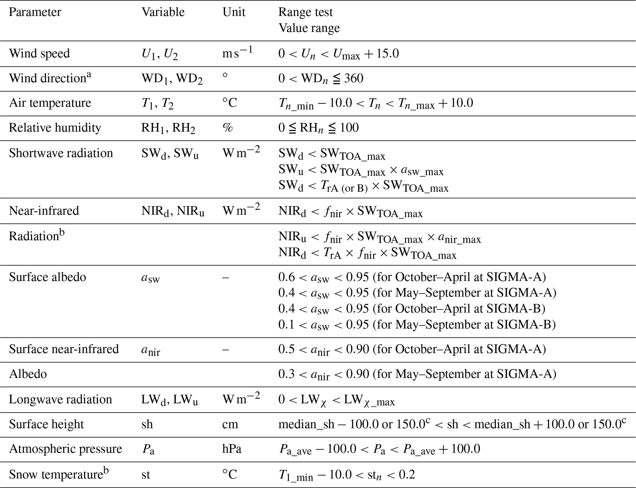
^a In the case of U_n>0. ^b Only SIGMA-A site. ^c The margin is changed depending on a variation of the data record in each applied period.

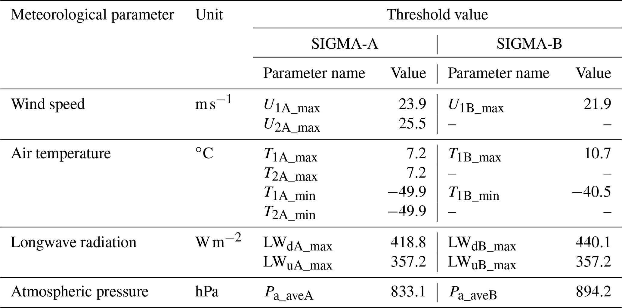
Table 4 Statistical values used in the range tests, determined from the entire observation period up to 31 August 2020.

4.1.1 Wind speed and wind direction

U_max used in the range test is the maximum value between the beginning of the observations and 31 August 2020, and +15.0 m s⁻¹ was taken as the range margin for the upper limit of U_n. In addition to the range test, the following basic processing was also performed. When U_n was zero (no wind), WD_n was flagged as erroneous:

$$\begin{array}{}\text{(11)}& U_n=\mathrm{0}\text{ and }{\text{WD}}_n>\mathrm{0}\to {\text{WD}}_n\text{ flagged }-\mathrm{9999}.\end{array}$$

When WD_n had a negative value, it was flagged as erroneous:

$$\begin{array}{}\text{(12)}& {\text{WD}}_n\le \mathrm{0}\to {\text{WD}}_n\text{ flagged }-\mathrm{9999}.\end{array}$$

4.1.2 Air temperature and relative humidity

T_{n_max} and T_{n_min} were determined from the entire observation period. The range margin for T_n was set as ±10.0 ^∘C. Discrepancies arising from the dual sensors at SIGMA-A were addressed in the secondary control (see Sect. 4.2.2).

4.1.3 Shortwave and near-infrared radiation

The main objective of the initial control for shortwave radiation was to mask erroneous records attributed to zero offset (Behrens, 2021). Zero offset is a few watts of radiation that occur at night, caused by the slight temperature difference between the two detectors (inside of the dome shelter and sensor body). However, since the value is an observation error, the observed value may be different from the original radiation balance and may need to be masked.

The range test is based on the assumption that SW_d cannot exceed the maximum of SW_TOA (SW_{TOA_max}) during the observation period (761.6 W m⁻² at SIGMA-A and 772.2 W m⁻² at SIGMA-B), and albedos a_sw and a_nir cannot be higher than a_{sw_max} and a_{nir_max} (a_{sw_max}=0.95 and a_{nir_max}=0.90), respectively, as determined from the radiative transfer model calculation (Aoki et al., 2003). Moreover, the fraction of the near-infrared spectral domain at the top of the atmosphere (f_nir) is assumed to be equal to 0.5151 based on the extraterrestrial spectral solar radiation (Wehrli, 1985). Based on those assumptions, upward and downward radiation fluxes were flagged as erroneous according to the range tests in Table 3.

The following procedures were also applied to mask erroneous records due to zero offset. These parameters were flagged as erroneous (−9999) in a subsequent case (using SW_χ as an example):

$$\begin{array}{}\text{(13)}& {\displaystyle }{\text{SW}}_{\mathit{\chi }}<\mathrm{0}\text{ and }\text{solz}<\mathrm{90.0}\to {\text{SW}}_{\mathit{\chi }}\text{ flagged }-\mathrm{9999},\text{(14)}& {\displaystyle }{\text{SW}}_{\mathit{\chi }}<\mathrm{0}\text{ and }\text{solz}\ge \mathrm{90.0}\to {\text{SW}}_{\mathit{\chi }}=\mathrm{0}.\end{array}$$

4.1.4 Longwave radiation

The range tests were performed for LW_d and LW_u under the conditions in Table 3. LW_{d_max} and LW_{u_max} were determined as follows:

$$\begin{array}{}\text{(15)}& {\displaystyle }{\text{LW}}_{\text{d\_max}}={\mathit{\epsilon }}_{\text{max}}\mathit{\sigma }{T}_{\text{max}},\text{(16)}& {\displaystyle }{\text{LW}}_{\text{u\_max}}=\mathit{\epsilon }\mathit{\sigma }{T}_{\text{s\_max}}.\end{array}$$

However, T_max is T_{2A_max} for the SIGMA-A site and T_{1B_max} for the SIGMA-B site. Maximum values were determined under the following assumptions: (1) T_2A and T_1B cannot be larger than T_{2A_max} and T_{1B_max}, respectively; (2) atmospheric emissivity is set to unity (ε_max); and (3) the value of LW_{u_max} is determined as the amount of radiation corresponding to longwave emission at T_{s_max} (=10 ^∘C), which includes errors due to longwave emissions from the poles of the AWS system and similar sources and the fact that the emissivity of the snow or ice surface (ε) is 0.98 (Armstrong and Brun, 2008).

Both upward and downward longwave fluxes were considered to be erroneous when the sensor appeared to be covered with snow or frost:

$$\begin{array}{}\text{(17)}& \begin{array}{rl}|{\text{LW}}_{\mathrm{d}}-{\text{LW}}_{\mathrm{u}}|\le \mathrm{1.0}\to {\text{LW}}_{\mathrm{d}}& \text{ and }{\text{LW}}_{\mathrm{u}}\\ & \text{ flagged }-\mathrm{9998}.\end{array}\end{array}$$

4.1.5 Surface height

The range test for surface height (sh) was imposed separately for each period between maintenances of the SIGMA-A site, when the main mast extension was adjusted to prevent the sensors from being buried in snow. A single range test sufficed for SIGMA-B. For each test, the range was set so that sh varied from the median by ±100 or ±150 cm, a margin that was determined depending on the variation of the data records in each period. The objective of this range test (Table 3) was to mask the most obvious outliers. In addition, corrections were made to the sh records after each of the three maintenance visits to the AWS at SIGMA-A.

4.1.6 Atmospheric pressure

P_{a_ave} used in the range test is the average atmospheric pressure for the observation period at each AWS site (Table 3). The additional margin that defined the range was ±100 hPa.

4.1.7 Snow temperature

The range test for snow temperature was conducted using the following threshold values: T_{1_min} is the minimum air temperature for the site, and the upper threshold, 0.2 ^∘C, incorporates the sensor's absolute error of 0.15 ^∘C and the requirement that the snow temperature cannot be positive.

4.2 Secondary QC for level-1.3 datasets

The secondary control applies another range test, an anomaly test, and a manual mask procedure. The range test sets a more precise variation range than the initial control and masks erroneous data records. The anomaly test sets a median and standard deviation (SD), which govern statistical tests as follows:

$$\begin{array}{}\text{(18)}& \mathit{\beta }<\text{median\_}\mathit{\beta }+\text{SD\_}\mathit{\beta }\times \mathit{\gamma },\end{array}$$

where β is an arbitrary variable, and the multiplier γ is 1, 2, or 3 depending on the intensity of the anomaly variation and is determined based on the test results in each case. Those statistical values and multipliers can be found in the QC program (archived at Nishimura et al., 2023g). This study determined the possible range of correct values in the level-1.2 dataset and identified and masked outliers if the variable deviated from its normal range. The manual mask procedure identifies and masks any remaining erroneous records. As a result of data masking by the initial control and the secondary control, the percentage of unmasked records for each parameter at the three data levels is shown in Table 5, and the effects of the two controls are illustrated in Fig. 3 and described in detail below.

Table 5 Percentage of unmasked data for each parameter in each dataset.

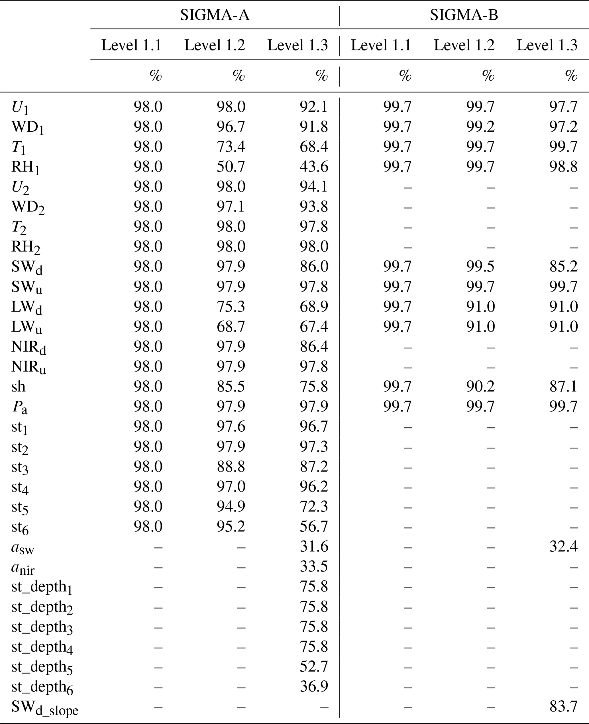
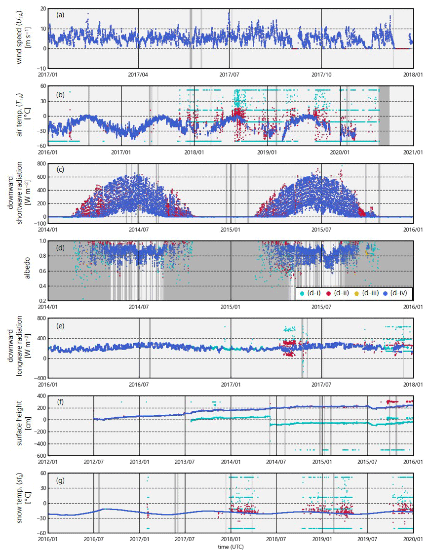
Figure 3 Examples of the initial and secondary controls for the SIGMA-A site: (a) wind speed (U_1A), (b) air temperature (T_1A), (c) downward shortwave radiation, (d) surface albedo, (e) downward longwave radiation, (f) surface height, and (g) snow temperature (st₃). In all panels except (d), the dark-gray areas represent time periods in which data records in the level-1.0 dataset were masked to produce the level-1.1 dataset, light-blue dots denote records masked by the initial control, red dots denote records masked by the secondary control, and dark-blue dots are the level-1.3 data records. In panel (d), the gray-shaded area represents the masked (−9999) data records that cannot be calculated due to the absence of masked SW_d or for other reasons. The light-blue, red, and yellow dots represent data points masked by three QC operations during the secondary control; see Sect. 4.2.4 for an explanation.

4.2.1 Wind speed and wind direction

When U_n was zero for more than 6 continuous hours, U_n and WD_n were both flagged as erroneous (−9999) under the assumption that the wind sensor was blocked by snow and ice. Although the initial control eliminated no U_n records, this step masked many values in the winter (Fig. 3a).

4.2.2 Air temperature and relative humidity

Anomaly tests for air temperature and relative humidity were only applied to the lower-level sensor records for SIGMA-A (i.e., T_1A and RH_1A). The anomaly test compared the difference (ΔT and ΔRH) between readings of the upper and lower sensors (i.e., $|T_{\text{1A}}-T_{\text{2A}}|$ and $|{\text{RH}}_{\text{1A}}-{\text{RH}}_{\text{2A}}|$) to the respective medians and SDs of those parameters. The medians were calculated from the data before 1 September 2017 because the data after that date appeared to include many erroneous T_1A records due to deterioration of the data logger or sensor. The SD criterion (γ in Eq. (18)) was adjusted modestly (γ=3) before 1 September 2017 and more stringently (γ=1) to detect outliers in the records of T_1A and RH_1A after that date; these were flagged as erroneous (−9999). The effectiveness of this adjustment is shown in Fig. 3b.

4.2.3 Shortwave and near-infrared radiation

The anomaly test for shortwave and near-infrared radiation was intended to mask the noise resulting from a weak electric pulse at large solar zenith angles. The median and SD values were calculated only from the records (SW_d, SW_u, NIR_d, and NIR_u) at $\text{solz}>\mathrm{90.0}{}^{\circ }$ to distinguish this noise source according to Eq. (18) for the above parameters, where γ=3. If the record is within its anomaly range, the records were identified as noise and modified to zero.

The downward-radiation components were sometimes overestimated as a result of icing or riming over the glass dome of the pyranometer. To mask these erroneous values, we applied range tests based on SW_TOA and threshold values of atmospheric transmittance for each site T_rA and T_rB (T_rA=0.881 and T_rB=0.872) calculated by a radiative transfer model (Aoki et al., 1999, 2003) shown in Table 3. Values of SW_d and NIR_d that were outside the range were flagged as erroneous (−9999).

To recognize other instances when the radiation sensor was covered with snow or frost, SW_d and NIR_d records corresponding to the following case where downward radiation is smaller than upward radiation were flagged as erroneous (−9998) using SW_χ as an example:

$$\begin{array}{}\text{(19)}& {\text{SW}}_{\mathrm{d}}<{\text{SW}}_{\mathrm{u}}.\end{array}$$

Figure 3c shows that the initial control eliminated a few erroneous SW_d data recorded in August 2015, whereas the secondary control masked many records, especially in February–May, that were affected by riming or frost.

4.2.4 Shortwave and near-infrared albedo

We calculated albedos a_sw and a_nir from the SW_d and NIR_d datasets that passed the secondary control. This calculation was done in four separate steps, shown by the colors of the dots in Fig. 3d.

1. Flagging for low pyranometer sensitivity

   At solar zenith angles near 90.0^∘, SW_d and NIR_d may not be accurate measurements because of the low sensitivity of the pyranometer. We therefore masked a_sw and a_nir values at $\text{solz}>\mathrm{85.0}{}^{\circ }$ or when the SW_d (NIR_d) value was below the median SW_d (NIR_d) value for $\text{solz}>\mathrm{85.0}{}^{\circ }$. Records masked in this step are shown in Fig. 3d as light-blue dots (d-i).

2. Range test for cold and warm periods

   The range test used the upper and lower thresholds for a_sw and a_nir shown in Table 3, as determined by the radiative transfer calculation of Aoki et al. (2003, 2011) plus a small error margin. Those thresholds correspond to the assumed surface conditions during two parts of the year. For the cold period of October–April, we used the lower thresholds for dry snow at the SIGMA-A site and dry or wet snow at the SIGMA-B site conditions. For the warm period of May–September we used the thresholds for wet snow at the SIGMA-A site and wet snow or dark ice at the SIGMA-B site. Records with albedo values beyond these theoretical thresholds were masked.

3. Anomaly test in low-atmospheric-transmittance condition

   The range test was augmented by an anomaly test to identify underestimates of a_sw and a_nir when SW_d (NIR_d) was low and when atmospheric transmittance (t_r) was small, typically at large solar zenith angles. We masked a_sw (a_nir) values that were unnaturally low owing to low t_r and SW_d (NIR_d) in the $\text{solz}>\mathrm{80.0}{}^{\circ }$ condition. Data records that were masked in either the range or anomaly tests are shown in Fig. 3d as red dots (d-ii).

4. Final steps

   In cases where LW_d was flagged as −9998 during the initial control (see Sect. 4.1.4), a_sw and a_nir were flagged as −9999 under the assumption that the radiation sensors were covered with snow or frost. The final step was a manual mask procedure. Data records that were masked in this phase are shown in Fig. 3d as orange dots (d-iii), and the final level-1.3 dataset is displayed with blue dots (d-iv).

4.2.5 Longwave radiation

The anomaly test for LW_d and LW_u was conducted only for the SIGMA-A dataset using a standard longwave radiant flux (LW_std), a measure of the amount of longwave radiation from the near-surface atmosphere that was calculated from the air temperature measurement by Brock and Arnold (2000):

$$\begin{array}{}\text{(20)}& {\displaystyle }{\text{LW}}_{\text{std}}={\mathit{\epsilon }}^{\ast }\mathit{\sigma }(T_{\text{2A}}+\mathrm{273.15}{)}^{\mathrm{4}},\text{(21)}& {\displaystyle }{\mathit{\epsilon }}^{\ast }=\left(\mathrm{1}+\mathit{\kappa }n\right){\mathit{\epsilon }}_{\mathrm{0}},\text{(22)}& {\displaystyle }{\mathit{\epsilon }}_{\mathrm{0}}=\mathrm{8.733}\times {\mathrm{10}}^{-\mathrm{3}}\times (T_{\text{2A}}+\mathrm{273.15}{)}^{\mathrm{0.788}},\end{array}$$

where ε^∗ is the atmospheric emissivity, σ ($=\mathrm{5.670}\times {\mathrm{10}}^{-\mathrm{8}}$) is the Stefan–Boltzmann constant, κ (=0.26) is a constant depending on cloud type (Braithwaite and Olesen, 1990), n is the cloud cover amount (n: [0,1] and set at 0.5 because it could not be determined), and ε₀ is the clear-sky emissivity. We assumed that LW_std was a close approximation of the true longwave radiant fluxes and used the absolute difference between LW_std and LW_d or LW_u (i.e., ΔLW_d or ΔLW_u) and its median and SD as the basis of the anomaly test, as in Eq. (18).

Because parts of the LW_d dataset contained many erroneous records attributed to degradation of the data logger (see Fig. 3e), we reduced the SD criterion (γ=1) in the period of 7 April to 7 June 2017 and after 1 September 2017. Except for those two periods, γ was set to 2 for both ΔLW_d and ΔLW_u. LW_d and LW_u records that were outliers under the criteria were flagged as erroneous (−9999). Figure 3e shows that the initial control (see Sect. 4.1.4) improved this anomaly test's efficacy, and the secondary control yielded a clean LW_d time series.

4.2.6 Surface height

The anomaly test for surface height masked data that displayed unrealistic fluctuations. Differences (Δsh) were determined with respect to mean and SD values from the preceding 72 h values during period 1, before 1 September 2017 (sh_mean1), and period 2, after 1 September 2017 (sh_mean2). The Δsh values were compared to the median plus the SD of Δsh for that period. In period 1, the SD criterion in Procedure 2.0.1 was strict (γ=1), and in period 2, the criterion was relaxed (γ=3). In addition, because surface height increased steadily in period 2, we derived the regression equation for this increase and identified outliers with respect to the SD of the regression, i.e., Δsh_reg, as follows:

$$\begin{array}{}\text{(23)}& \mathrm{\Delta }{\text{sh}}_{\text{reg}}<{\text{SD}}_{\text{reg}}\text{\_sh}\mathrm{\text{for after 1 September 2017}}.\end{array}$$

Records of sh that varied beyond the anomaly ranges were flagged as erroneous (−9999).

A manual mask procedure was added as a final step. The result of the QC procedure is shown in Fig. 3f. The initial control, which corrected gaps resulting from the AWS maintenance (see Sect. 4.1.5), yielded the smoothed data record that enabled the application of the anomaly test. The sensor height dataset was made using the initial sensor height (3 or 6 m) and the QC-completed temporal surface height data. Therefore, the QC for sensor height data has already been implemented through the QC for surface height data.

4.2.7 Snow temperature

In the first step, data records were masked when the snow temperature sensor was suspected to be located above the snow surface:

$$\begin{array}{}\text{(24)}& {\text{st\_depth}}_n<-\mathrm{1.0}\to {\text{st}}_n\text{ flagged }-\mathrm{9999},\end{array}$$

where st_depth_n (cm) was calculated using surface height data and the initial setting depth of sensor n (see Sect. 3). The threshold of st_depth_n included a margin of 1.0 cm to reflect the accuracy of the surface height sensor. The st_n was flagged as −9997 if we could not judge whether the snow temperature sensor was located below the snow surface.

The anomaly test for st_n consisted of two procedures. The first procedure relied on a temperature gap (Δst_d1) between st₄ and data from each of the other five levels (st_not4) (i.e., $\mathrm{\Delta }{\text{st}}_{\text{d1}}=|{\text{st}}_{\mathrm{4}}-{\text{st}}_{\text{not4}}|$) because st₄ had very few erroneous data. The SD criterion (γ) for this anomaly test was changed for each parameter depending on the variability of the data. The second procedure used the difference (Δst_d2) between st_n and its mean value st_{n_mean} from the previous 72 h ($\mathrm{\Delta }{\text{st}}_{\text{d2}}=|{\text{st}}_n-{\text{st}}_{n\text{\_mean}}|$), calculated using the same method as sh_mean (see Sect. 4.2.6). The SD criteria (γ) were all at unity in this test. In both procedures, the median and SD terms were calculated from records for the full time period. Records detected as outliers were flagged as −9999. Figure 3g shows the results of all procedures using st₃ as an example.

4.2.8 Atmospheric pressure

The time series of P_a included only a few erroneous records. We masked outliers on the basis of

$$\begin{array}{}\text{(25)}& \left|P_{\mathrm{a}}-P_{\text{a\_mean}}\right|>\mathrm{20.0},\end{array}$$

where P_{a_mean} is the average for the past 3 h (excluding masked data records). We set the threshold at 20.0, a higher value than the SD, because using the SD could have masked valid records. This threshold value of 20 hPa is based on the assumption that a 20 hPa pressure jump is unlikely to occur in a few hours. This procedure was successful in only masking erroneous data of both sites.

5 Temporal variations of meteorological parameters

This section shows the results of simple analyses of the level-1.3 dataset.

5.1 Air temperature and surface height

Figure 4 shows the air temperature fluctuations and surface height (sh) variations at both sites. Mean air temperatures (2013–2019) were −18.1 ^∘C at the SIGMA-A site and −12.3 ^∘C at the SIGMA-B site. The annual maxima of monthly data were recorded every July at both sites, except for August 2019 at the SIGMA-B site. At the SIGMA-A site, the annual maximum in 2015 was slightly positive (+0.1 ^∘C in July), but others were negative. At the SIGMA-B site, these were above freezing in all years. The annual minima occurred in different months between December and March. Unusually high hourly temperatures were recorded in mid-July 2015 (7.2 ^∘C at SIGMA-A and 10.7 ^∘C at SIGMA-B). Air temperatures exceeding 5.0 ^∘C at SIGMA-A and 10.0 ^∘C at SIGMA-B were common during that period.

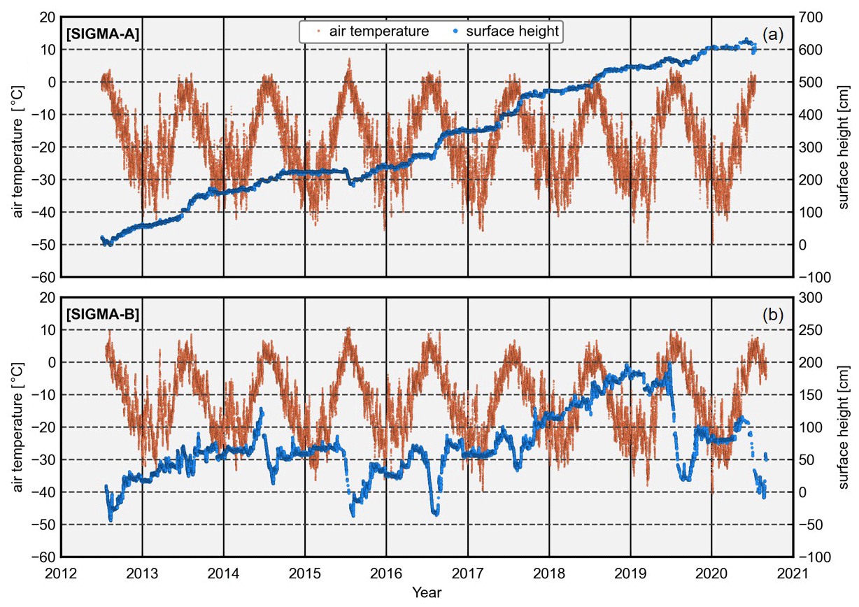
Figure 4 Time series of hourly air temperature and surface height at the (a) SIGMA-A (showing T₂ data) and (b) SIGMA-B sites.

Surface height steadily increased at the SIGMA-A site during the 8-year study period (Fig. 4), in which sh rose approximately 1 m in the mass balance years (September to August) of 2013–2014, 2016–2017, and 2017–2018, and decreased slightly in the summers of 2011–2012, 2014–2015, and 2019–2020. Accumulations were notable in fall and relatively small in winter. At the SIGMA-B site, in contrast, increases and decreases in sh were observed during each mass balance year. Decreases in sh during summers were rare during the summers of 2012-2013 and 2017–2018 but common during the 2013–2014, 2014–2015, 2015–2016, 2018–2019, and 2019–2020 summers, when decreases were greater than 1 m.

5.2 Atmospheric pressure and seasonal variation of temperature lapse rate

The time series of atmospheric pressure (P_a) at the SIGMA-A and SIGMA-B sites show a clear seasonal variation, being high in summer and low in winter (Fig. 5). The two data records had similar variation patterns that were strongly correlated (r=0.98). The mean values for the whole observation period were 833.1 hPa at site SIGMA-A and 894.2 hPa at site SIGMA-B (Table 4). The difference in monthly mean P_a between the sites was smaller in summer and larger in winter (Fig. 6), and the amplitude of the annual cycle was greater at the SIGMA-A site.

Figure 5 Time series of hourly atmospheric pressure (P_a) at the SIGMA-A and SIGMA-B sites.

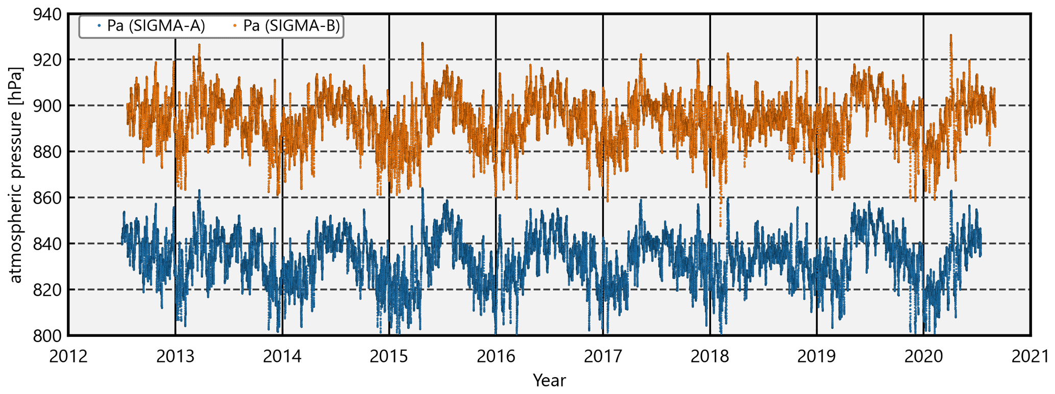
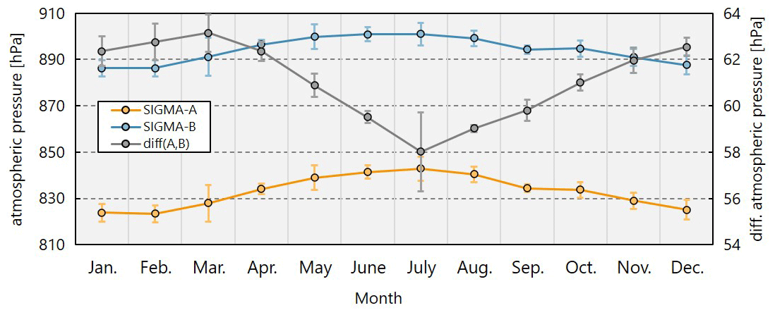
Figure 6 Time series of ensemble averages of monthly mean atmospheric pressures during all years at both sites and their difference. Error bars indicate ±1 SD.

5.3 Albedo

Whereas shortwave albedo (a_sw) was rarely lower than 0.7 at site SIGMA-A, near-infrared albedo (a_nir) was below 0.6 in 2012, 2015, 2016, 2019, and 2020 (Fig. 7). Because a_nir depends on the snow grain size (Wiscombe and Warren, 1980), this finding implies that snow metamorphism progressed at the SIGMA-A site in those years (Hirose et al., 2021). A strong decrease in a_sw was observed at the SIGMA-B site during those same summers, which corresponded to notable decreases in surface height (Fig. 4b). The decreases in albedo may have accelerated snowmelt and caused the decreases in surface height at SIGMA-B during the warm summers of those years (see Sect. 5.1). It appears that the difference in albedo reduction between the SIGMA-A and SIGMA-B sites in summer originated from the difference in air temperature between the sites.

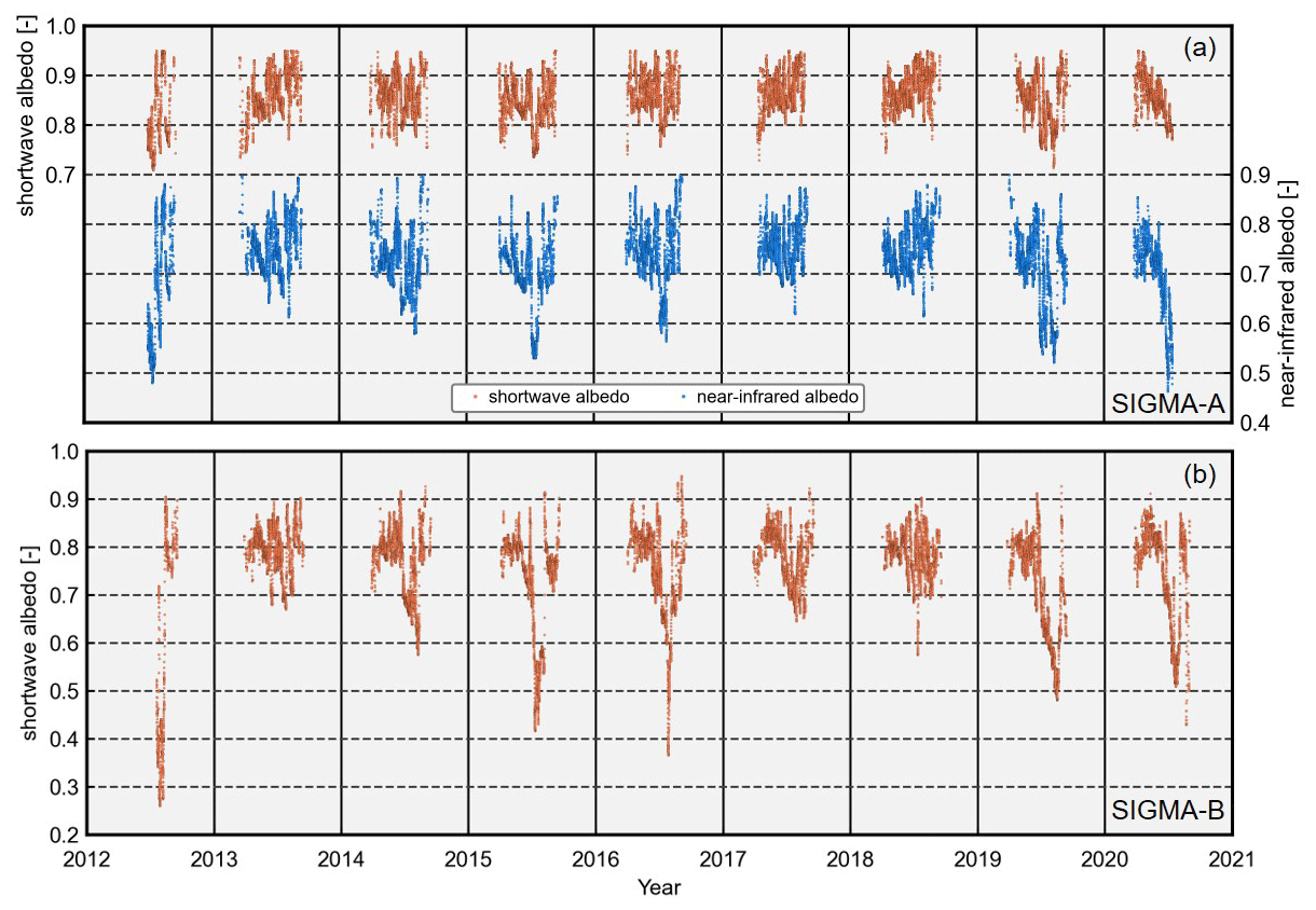
Figure 7 Time series of hourly shortwave and near-infrared albedos at the (a) SIGMA-A and (b) SIGMA-B sites.

5.4 Snow temperature

Figure 8 shows the time series of snow temperatures (st₁–st₆) and snow sensor depths (st_depth_1–6). The sensor depths were calculated from each sensor's initial depths (see Sect. 3.1) and the surface height variations at the SIGMA-A site. Seasonal and short-term snow temperature fluctuations were observed, which became smaller after the 2016–2017 winter season, when snow accumulation was very large (Fig. 4). We assumed that the sensors were buried more deeply at that time, resulting in smaller fluctuations in snow temperature. The annual mean snow temperatures after 2016, a year in which snow temperatures were relatively stable and less variable, were between $-\mathrm{18.9}\pm \mathrm{0.5}$ (st₄) and $-\mathrm{19.5}\pm \mathrm{1.7}$ ^∘C (st₅).

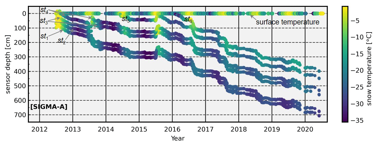
Figure 8 Time series of hourly snow temperatures (st₁–st₆), sensor depth, and surface temperature (calculated from upward longwave radiation) at the SIGMA-A site.

Sensors recorded relatively high snow temperatures when they were positioned at shallow depths below the snow surface. However, in the summer of 2015, sensors st₃ and st₄ registered 0 ^∘C even though they were more than 1 m below the snow surface. Air temperatures above freezing and a large decrease in surface height were observed in this period (Fig. 4); thus, it is plausible that snowmelt occurred from the surface to depths near 120 cm, where st₃ was located at that time.

5.5 Longwave radiation

The frequency distribution of longwave radiation, taken to represent the atmospheric condition, is often used as an indicator of climatological cloudiness (Stramler et al., 2011). Figure 9 shows the histograms of the occurrence frequency of downward (LW_d) and net longwave radiation (${\text{LW}}_{\text{net}}={\text{LW}}_{\mathrm{d}}-{\text{LW}}_{\mathrm{u}}$) during July of all years at the SIGMA-A and SIGMA-B sites. The corresponding histograms for the four seasons (fall: SON, winter: DJF, spring: MAM, summer: JJA) are shown in Figs. S1 and S2 in the Supplement. The July LW_d data from both sites had bimodal distributions, with a lower mode of 220–240 W m⁻² at SIGMA-A and 240–260 W m⁻² at SIGMA-B and a higher mode of 290–310 W m⁻² at SIGMA-A and 310–330 W m⁻² at SIGMA-B. The histograms of July and seasonal LW_net had similar but clearer bimodal distributions, with modes at approximately 0 and −70 W m⁻² (Figs. 9c and d and S2).

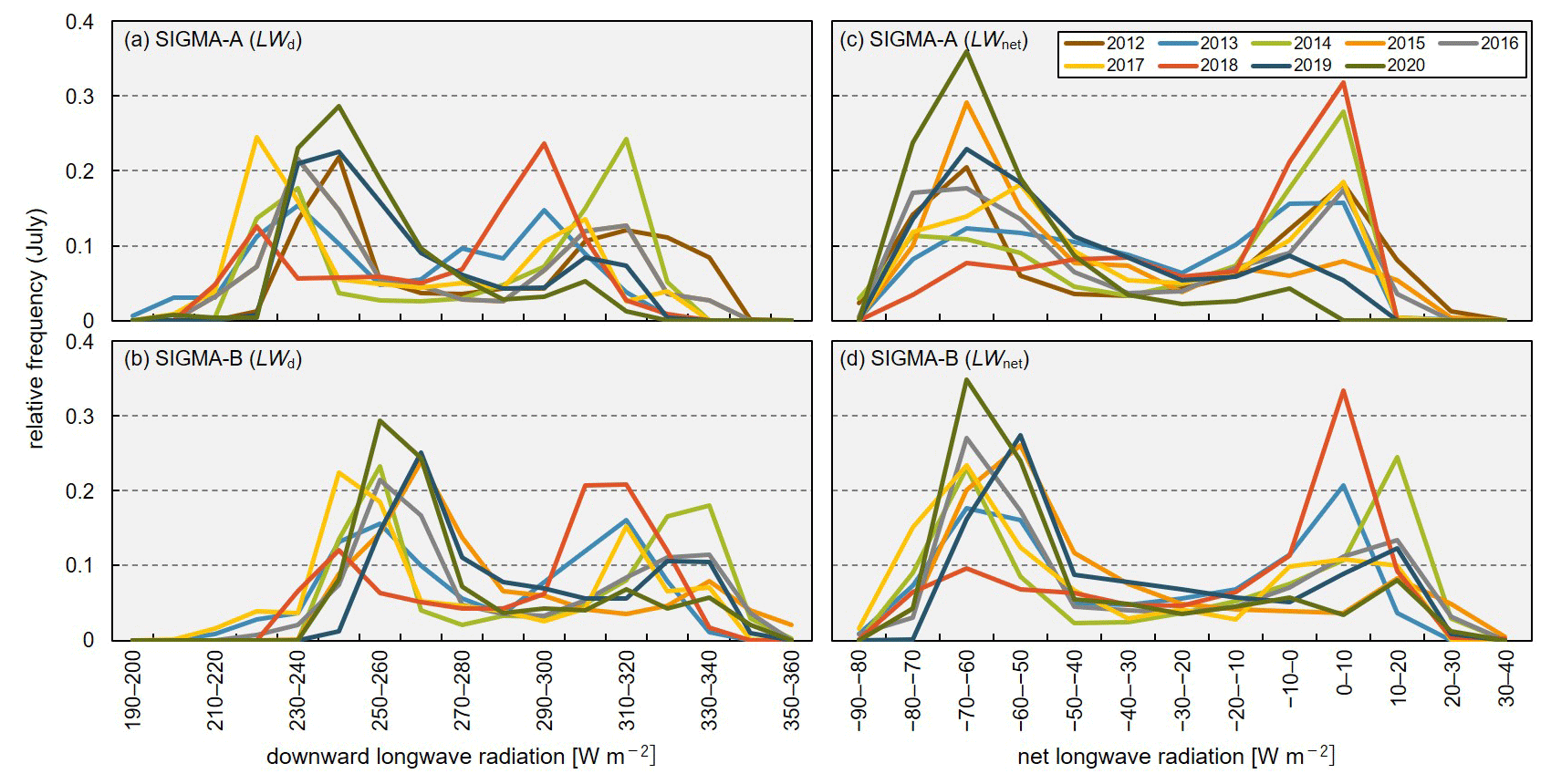
Figure 9 Histograms of the occurrence frequency of hourly downward longwave radiation (LW_d) and net longwave radiation (LW_net) observed at the SIGMA-A and SIGMA-B sites in July of all years in the study period. Each relative frequency represents the fraction of the total contained in each 10 W m⁻² bin.

LW_net can be regarded as an indicator of cloudiness because blackbody radiation from the cloud cover increases both downward and net longwave radiation. Stramler et al. (2011) and Morrison et al. (2012) have argued that surface net longwave radiative flux has two modes in terms of occurrence frequency (at −40 and 0 W m⁻²), which correspond to clear-sky and overcast (low-level mixed-phase clouds) conditions. In overcast conditions, because the cloud base and the surface are in thermal equilibrium, the vertical thermal gradient is small, and the longwave radiation budget is balanced (LW_net=0 W m⁻²) at the surface. The two modes of LW_net (0 and −70 W m⁻²) at the two AWS sites appear to correspond to the modes proposed by these earlier studies.

The occurrence frequency of LW_net in JJA appears to be more variable than those for the other seasons at both sites (Fig. S2). In these months, the air temperature rises, and sea ice extent decreases, increasing the water vapor supply and advection from the surrounding sea to coastal Greenland (Kim and Kim, 2017; Liang et al., 2022). In such atmospheric conditions, the cloud formation process is susceptible to synoptic-scale disturbances. The histogram of LW_net for July (Fig. 9) indicates a higher frequency of clear-sky conditions (LW${}_{\text{net}}\cong -\mathrm{70}$ W m⁻²) in 2015, 2019, and 2020 and overcast conditions (LW_net≅0 W m⁻²) in 2014 and 2018. In SON and MAM, the weather conditions were less variable, and overcast and clear-sky conditions dominated, respectively. Our analysis shows that cloudiness in JJA was more variable than in other seasons, a result that is also borne out by satellite observations (Ryan et al., 2022).

6 Data availability

The level-1.1 (SIGMA-A; https://doi.org/10.17592/001.2022041301, Nishimura et al., 2023d, SIGMA-B; https://doi.org/10.17592/001.2022041304, Nishimura et al., 2023a), level-1.2 (SIGMA-A; https://doi.org/10.17592/001.2022041302, Nishimura et al. 2023e, SIGMA-B; https://doi.org/10.17592/001.2022041305, Nishimura et al., 2023b), and level-1.3 (SIGMA-A; https://doi.org/10.17592/001.2022041303, Nishimura et al., 2023f, SIGMA-B; https://doi.org/10.17592/001.2022041306, Nishimura et al., 2023c) datasets from this study are archived and available from the Arctic Data archive System (ADS) in the National Institute of Polar Research (Table 6), where they are stored in text (CSV) file format. Detailed information on the data content is presented in the file data_format_site-name_data-level.csv associated with each of these dataset files.

Table 6 Information for the archived datasets from the SIGMA-A and SIGMA-B sites.

7 Summary and conclusion

This paper describes the in situ meteorological datasets from the SIGMA-A and SIGMA-B AWS sites in northwest Greenland and details the QC methods used in preparing the datasets. At this time when drastic environmental change is proceeding in the Arctic region, sound meteorological data and QC methods are of ever-growing importance.

The QC method offered here consists of two basic steps. The first step, the initial control, masks observations that are affected by mechanical malfunctions or local phenomena and is a pre-treatment for the second QC step. This step uses simple statistics to set the range of permissible variation in northwest Greenland for each observational parameter and flags erroneous records on the basis of that variation range. The second QC step, the secondary control, masks erroneous observations based on more stringent variation ranges as determined by the median and SD values of the full observation record. The QC procedures offered here may be valuable for scientists developing their own QC efforts.

We presented examples of time series of air temperature, surface height, atmospheric pressure, snow temperature, surface albedos, and longwave radiation based on the resulting hourly meteorological dataset for 2012–2020 in northwest Greenland. We also extracted information on climatological cloudiness based on LW_net data derived from these in situ ground observations. Our primary findings are summarized in the following four points: (1) high air temperature in the 2015 summer and low surface albedos in 2016, 2019, and 2020 summers were recorded at both SIGMA-A and SIGMA-B sites. (2) Apparent decreases in surface height occurred in 2015 at both AWS sites and in 2016, 2019, and 2020 at the SIGMA-B site. (3) Observed atmospheric conditions in JJA were relatively variable in northwest Greenland compared to in the other seasons. (4) Frequent clear-sky conditions typified the summers of 2015, 2019, and 2020.

The datasets described here are archived in the open-access Arctic Data archive System for all scientific communities. We anticipate that they will not only aid in understanding and monitoring the current climate in northwest Greenland but also contribute more broadly to the advancement of polar climate studies.