A global 5 km monthly potential evapotranspiration dataset (1982–2015) estimated by the Shuttleworth–Wallace model

As the theoretical upper bound of evapotranspiration (ET) or water use by ecosystems, potential ET (PET) has always been widely used as a variable linking a variety of disciplines, such as climatology, ecology, hydrology, and agronomy. However, substantial uncertainties exist in the current PET methods (e.g., empiric models and single-layer models) and datasets because of unrealistic configurations of land surface and unreasonable parameterizations. Therefore, this study comprehensively considered interspecific differences in various vegetation-related parameters (e.g., plant stomatal resistance and CO₂ effects on stomatal resistance) to calibrate and parametrize the Shuttleworth–Wallace (SW) model for forests, shrubland, grassland, and cropland. We derived the parameters using identified daily ET observations with no water stress (i.e., PET) at 96 eddy covariance (EC) sites across the globe. Model validations suggest that the calibrated model could be transferable from known observations to any location. Based on four popular meteorological datasets, relatively realistic canopy height, time-varying land use or land cover, and the leaf area index, we generated a global 5 km ensemble mean monthly PET dataset that includes two components of potential transpiration (PT) and soil evaporation (PE) for the 1982–2015 time period. Using this new dataset, the climatological characteristics of PET partitioning and the spatiotemporal changes in PET, PE, and PT were investigated. The global mean annual PET was 1198.96 mm with $\mathrm{PT}/\mathrm{PET}$ of 41 % and $\mathrm{PE}/\mathrm{PET}$ of 59 %, controlled moreover by PT and PE of over 41 % and 59 % of the globe, respectively. Globally, the annual PET and PT significantly (p<0.05) increase by 1.26 and 1.27 mm yr⁻¹ over the last 34 years, followed by a slight decrease in the annual PE. Overall, the annual PET changes over 53 % of the globe could be attributed to PT, and the rest to PE. The new PET dataset may be used by academic communities and various agencies to conduct climatological analyses, hydrological modeling, drought studies, agricultural water management, and biodiversity conservation. The dataset is available at https://doi.org/10.11888/Terre.tpdc.300193 (Sun et al., 2023).

1 Introduction

Potential evapotranspiration (PET) is the maximum amount of water that can be transferred to the air from a given land cover (e.g., land and water), providing an upper limit of the evaporative losses from this land cover (Allen et al., 1998; Milly and Dunne, 2016; Xiang et al., 2020). Commonly, it consists of potential evaporation from soils (PE) and/or transpiration by plants (PT) when the soil water supply for the evapotranspiration (ET) process is non-limiting (Thornthwaite, 1948; Xiang et al., 2020). The spatiotemporal differences in PET mainly depend on those of climatic conditions, including net radiation, wind speed, and the atmospheric vapor deficit, and thus PET is usually regarded as an accepted proxy for the atmospheric evaporative demand. Additionally, PET has been widely used to estimate actual ET (Sun et al., 2011a; Rao et al., 2011; C. Liu et al., 2017), a critical variable that links the water, energy, and carbon cycles (Sun et al., 2011b), and thus it is a key variable for a variety of disciplines, such as climatology, ecology, hydrology, and agronomy (Allen et al., 1998; Espadafor et al., 2011; Beven, 2012).

Historically, numerous PET models have been proposed (Singh and Xu, 1997; Xu and Singh, 2000, 2001; Xiang et al., 2020). In general, the PET models can be grouped into four types: mass-transfer-based ones (e.g., Dalton-type models in Table S1; Singh and Xu, 1997), which are based on Dalton's law and take observed wind speed and water vapor pressure as inputs; temperature-based ones (e.g., the Thornthwaite equation in Table S1; Thornthwaite, 1948), which take temperature as a proxy for the radiative energy available, along with extraterrestrial radiation estimated from the date of the year and latitude; radiation-based ones (e.g., the Turc and Hargreaves models in Table S1; Turc, 1961; Hargreaves and Samani, 1983), which use measured data such as net solar radiation, sunshine hours, or cloudiness factors; and combination ones (e.g., Penman–Monteith models, including their original types and variants in Table S1; Penman, 1948; Monteith, 1965; Allen et al., 1998), which combine the energy balance with the mass transfer method. Despite the low requirement of climatic variables for the former three types of the PET model, they lack comprehensive physical considerations of the ET process and heavily rely on empirical factors which are dependent on historical or present-day climate for calibration (Tabari and Talaee, 2011; Aschonitis et al., 2015; Tanguy et al., 2018; Xiang et al., 2020). By contrast, the combination models (e.g., the Penman–Monteith models) involve a relatively comprehensive physical basis and thus have been widely used by various scientific communities (McVicar et al., 2007; Mu et al., 2013; Sun et al., 2017, 2022). As one of the most famous Penman–Monteith model variants, the Food and Agriculture Organization of the United Nations (FAO)-56 Penman–Monteith model has been validated against lysimeter data across the globe, obtaining reliable results (Jensen et al., 1990; Itenfisu et al., 2000; Berengena and Gavilán, 2005; Trajkovic, 2007; X. Liu et al., 2017; Gong et al., 2017), and is recommended as a standard tool for calculating PET with climatic data by the International Commission on Irrigation and Drainage (ICID), the FAO, and the American Society of Civil Engineers (ASCE).

Despite the relatively satisfactory performance, the Penman–Monteith models still have inherent shortcomings for the parameterization scheme of the land surface. For example, these models set the evaporating and/or transpiration surfaces as a whole (i.e., a so-called “big leaf”), regardless of differences in the processes of soil evaporation and plant transpiration (Stannard, 1993; Yang and Shang et al., 2012; Liu et al., 2015). Over a large region, however, the big leaf assumption is rarely valid. Usually, many vegetation types co-exist over the land, and there are always some parts or periods where or when the vegetation is not “closed” (i.e., an open canopy where light can penetrate to the ground). The big leaf assumption potentially limits the applicability of the Penman–Monteith models under various vegetation distribution conditions, e.g., better (worse) performance under complete and homogeneous (sparse and inhomogeneous) vegetation distribution conditions (Shuttleworth and Wallace, 1985; Stannard, 1993; Yang and Shang, 2012; Huang et al., 2020). Comprehensively considering differences in the processes of soil evaporation and plant transpiration, Shuttleworth and Wallace (1985) extended the Penman–Monteith single-layer models to a two-layer model, i.e., the Shuttleworth–Wallace (SW) model. This model divided ET into plant and soil components based on surface resistances to regulate the heat and mass transfer from plant and soil surfaces and based on aerodynamic resistance to regulate fluxes into the atmosphere (Lagos et al., 2013; Liu et al., 2015; Zhao et al., 2015; Huang et al., 2020). Relative to the Penman–Monteith models, the SW model is the first analytical model combining transpiration and soil evaporation by formulating the different media via which evaporative flux travels as resistances (Kool et al., 2014). This partitioning is crucial for reasonably describing and understanding ET processes (Zhou et al., 2016, 2018). The SW model is generally considered to be more accurate and more physically based and has been extensively used at point and regional scales (Brisson et al., 1998; Hu et al., 2009; Kool et al., 2014; Liu et al., 2015; Huang et al., 2020).

It should be noted that there are two major difficulties in running the SW model. Firstly, it has a high requirement for meteorological data inputs, including the maximum and minimum air temperatures, relative humidity, wind speed and solar radiation, or their proxy data. Commonly, the maximum and minimum air temperatures are measured at meteorological sites, while observations of the other elements are scare, especially when long time series and large spatial coverage are required for climate studies. This may be a major reason for some temperature-based and radiation-based PET models (e.g., the Priestley–Taylor and Hargreaves–Samani models) still being widely used at present, especially for regions with sparse meteorological observations (Aschonitis et al., 2017; Tanguy et al., 2018). Secondly, the SW model is hard to parameterize given the large number of parameters (Brisson et al., 1998; Odhiambo and Irmak, 2011; Kool et al., 2014), and therefore this model is often applied at point and regional scales (Iritz et al., 1999; Yang and Shang, 2012; Liu et al., 2015; Huang et al., 2020; Chen et al., 2022). Fortunately, with the development of observation and numerical simulation technology during the past decades, various global datasets have become available, including meteorological datasets (e.g., Harris et al., 2020; Molod et al., 2015; Hersbach et al., 2020; Beck et al., 2022), vegetation height datasets (e.g., Simard et al., 2011; Wang et al., 2016; Potapov et al., 2020; Lang et al., 2021, 2022), land use and land cover (LULC) datasets (e.g., Liu et al., 2020a, b), leaf area index (LAI) datasets (e.g., Friedl et al., 2010; Liu et al., 2012; Zhu et al., 2013; Xiao et al., 2014), and eddy covariance (EC) flux observations across various ecosystems (e.g., LaThuile, https://fluxnet.org/data/la-thuile-dataset/, last access: 20 August 2022; FLUXNET2015, http://fluxnet.fluxdata.org/data/fluxnet2015-dataset/, last access: 30 August 2022.; OzFlux, https://data.ozflux.org.au/portal/home.jspx, last access: 15 June 2022.; and AsiaFlux, http://asiaflux.net/?page_id=23, last access: 21 July 2022). These released datasets provide a valuable opportunity for parameterizing and driving the SW model at the global scale.

Previous studies have suggested that land surface properties could play a dominant role in controlling variations of the ET process (Sun et al., 2021, 2022). Of the land surface properties, vegetation is the most ever-changing due to plant growth, natural disturbances, and anthropogenic disturbances (Q. Liu et al., 2016; Y. Liu et al., 2016; Papagiannopoulou et al., 2017; Cavalcante et al., 2019). Recently, with climate change and/or intensified human activities, vegetation has greatly changed on regional and even global scales (Zhu et al., 2016; Chen et al., 2019), including shifts in vegetation types and vegetation greening (i.e., increases in LAI or other vegetation indices), which have altered the allocation of available water and energy (Zhou et al., 2016, 2018; Sun et al., 2022). As an important biophysical parameter of vegetation, the plant stomatal resistance has been widely shown to increase with the elevated atmospheric CO₂ concentration by numerous observations and numerical simulations, but the increasing magnitudes differed among vegetation types (Wand et al., 1999; Medlyn et al., 2001; Norby et al., 2005; Franks and Beerling, 2008; Lin et al., 2015; Gardner et al., 2022). The increased plant stomatal resistance could in turn reduce plant transpiration and thereby change the water cycle on regional and even global scales (Gedney et al., 2006; Piao et al., 2007; Sun et al., 2014; Zhao and Cao, 2022; Zhan et al., 2022). In particular, such impacts of elevated CO₂-induced plant stomatal resistance increase on hydrological processes have proven to be of significance, especially for the future climate change scenarios with high CO₂ emissions (Roderick et al., 2015; Milly and Dunne, 2016; Scheff, 2018; Yang et al., 2019). This suggested that the temporal changes in vegetation (i.e., vegetation types, LAI, and plant stomatal resistance) should be incorporated into the models for accurate PET estimates. However, it is unfortunate that the various existing PET products, such as Climatic Research Unit (CRU) Time-Series (TS) 4.06 (CRU TS4.06; Harris et al., 2020), MOD16 (Running et al., 2017), the Global Land Evaporation Amsterdam Model (GLEAM) v3.6 (Miralles et al., 2011; Martens et al., 2017), the Priestley–Taylor Jet Propulsion Laboratory (PT-JPL) model (Fisher et al., 2011), and hPET (Singer et al., 2021), did not fully consider the impacts of such vegetation changes on PET, potentially resulting in biases of the estimates from the truth values and then introducing uncertainties into the studies based on these products. As a result, a new PET dataset based on more reasonable parameterizations and more realistic configurations of the land surface is needed.

By making use of various existing datasets, this study comprehensively considered spatiotemporal differences in land surfaces and elevated CO₂-induced biophysical effects on plant stomatal resistance to parameterize the SW model, and it produced a new global monthly PET dataset. Specifically, our objectives are (1) to calibrate the SW model with the EC flux observations to obtain key parameters for each LULC type and to evaluate the performance of the calibrated model, (2) to generate a global monthly PET product (including PE and PT) from 1982 to 2015 with the calibrated SW model and various inputs, and (3) to investigate the climatological characteristics of PET partitioning and the spatiotemporal changes in PET and its two components across the globe during 1982–2015.

2 Material and methods

2.1 Data sources

2.1.1 Eddy covariance measurements

To fully utilize the existing EC measurements, this study collected the half-hourly or hourly FLUXNET2015 Tier-2 (http://fluxnet.fluxdata.org/data/fluxnet2015-dataset/, last access: 30 August 2022), LaThuile (https://fluxnet.org/data/la-thuile-dataset/, last access: 20 August 2022), AsiaFlux (http://asiaflux.net/?page_id=23, last access: 21 July 2022), and OzFlux (https://data.ozflux.org.au/portal/home.jspx, last access: 15 June 2022) datasets. Following Maes et al. (2019), we processed the four datasets to provide the necessary inputs and the ET observations without water limits (i.e., PET) for calibrating the SW model.

First, we screened the measurements using data quality control. Sites lacking one or more of the basic measurements required for our analysis, i.e., latent heat (LE), sensible heat (H), soil heat flux (G), the net radiation fluxes (Rn), wind speed (u), air temperature, relative humidity (RH), actual vapor pressure (e_a), and atmospheric water concentration and vapor pressure deficit (D), were not considered further. Considering potential impacts of surface energy imbalance on the results, the corrected half-hourly or hourly LE and H (Pastorello et al., 2020) were used here. Regarding the major heat fluxes (LE, H, and G), good gap-filled records were retained according to the quality flags provided by the four datasets. When the flags for Rn observations were unavailable, the flags of the downward shortwave radiation were used instead. Mainly due to the impacts of interception loss and condensation on the accuracy of H or LE measurements (Mizutani et al., 1997), the negative values were masked out. Likewise, all Rn negative values were masked out.

Second, the half-hourly or hourly measurements were aggregated to daytime records. Only days on which more than 70 % of the basic data were measured directly were retained, and days with rainfall during midnight–sunset were excluded from the analyses to remove the effects of rainfall interception. Moreover, we only retained sites with 80 or more days for the processing below. Taking 5 W m⁻² of top-of-atmosphere incoming shortwave radiation as a minimum threshold, the half-hourly or hourly measurements were aggregated to daytime composites, and then the daytime values were obtained by subtracting measurements at the first and last (half-)hours for these aggregates.

Third, we identified days with no soil water limits. This study employed an energy-balance-based approach to select unstressed days rather than the soil moisture criterion. The major considerations were three-fold: (a) no soil moisture measurements existed at most of the EC sites; (b) the energy-balance-based method could effectively remove days on which the ecosystem is not limited by soil moisture availability but is stressed by other environmental factors (e.g., insect plagues, phenological leaf-out, fires, heat and atmospheric dryness stress, nutrient limitations); and (c) soil moisture may not be a good indicator of water stress due to variable rooting depth and its inaccurate measurements (Powell et al., 2006; Douglas et al., 2009; Martínez-Vilalta et al., 2014). The evaporative fraction, i.e., EF = $\mathit{LE}/(\mathit{LE}+H$), was selected as the energy balance criterion, and we assumed that under conditions of no water limits a larger fraction of the available energy should be used for evaporating water (Gentine et al., 2007, 2011; Maes et al., 2011). Taking a site as an example, a day was identified as having no water limits when its corresponding EF exceeded the 95th percentile EF threshold. Notably, if fewer than 15 d fulfilled this criterion at some particular sites, the 15 d with the highest EF were used as unstressed days.

Finally, the sites used for further analyses were selected. Despite the usage of the corrected half-hourly or hourly LE and H here, we found that an evident surface energy imbalance still existed in the daytime, with a Bowen ratio between 0.60 and 1.80. To further reduce the potential impacts of this issue, we retained records with a Bowen ratio between 0.90 and 1.10. After this, if a certain site had fewer than 8 unstressed days, it was removed. Because the LAI and the CO₂ concentration were unavailable at some sites, the Global LAnd Surface Satellite (GLASS) LAI and CO₂ concentration (${\mathit{\rho }}_{{\mathrm{CO}}_{\mathrm{2}}}$, ppm) observed at Mauna Loa were used instead. Finally, 96 sites were retained, including 73, 5, 3, and 18 sites from the FLUXNET2015 Tier-2, AsiaFlux, OzFlux, and LaThuile datasets, respectively (Fig. 1). Their basic information is shown in Table S2.

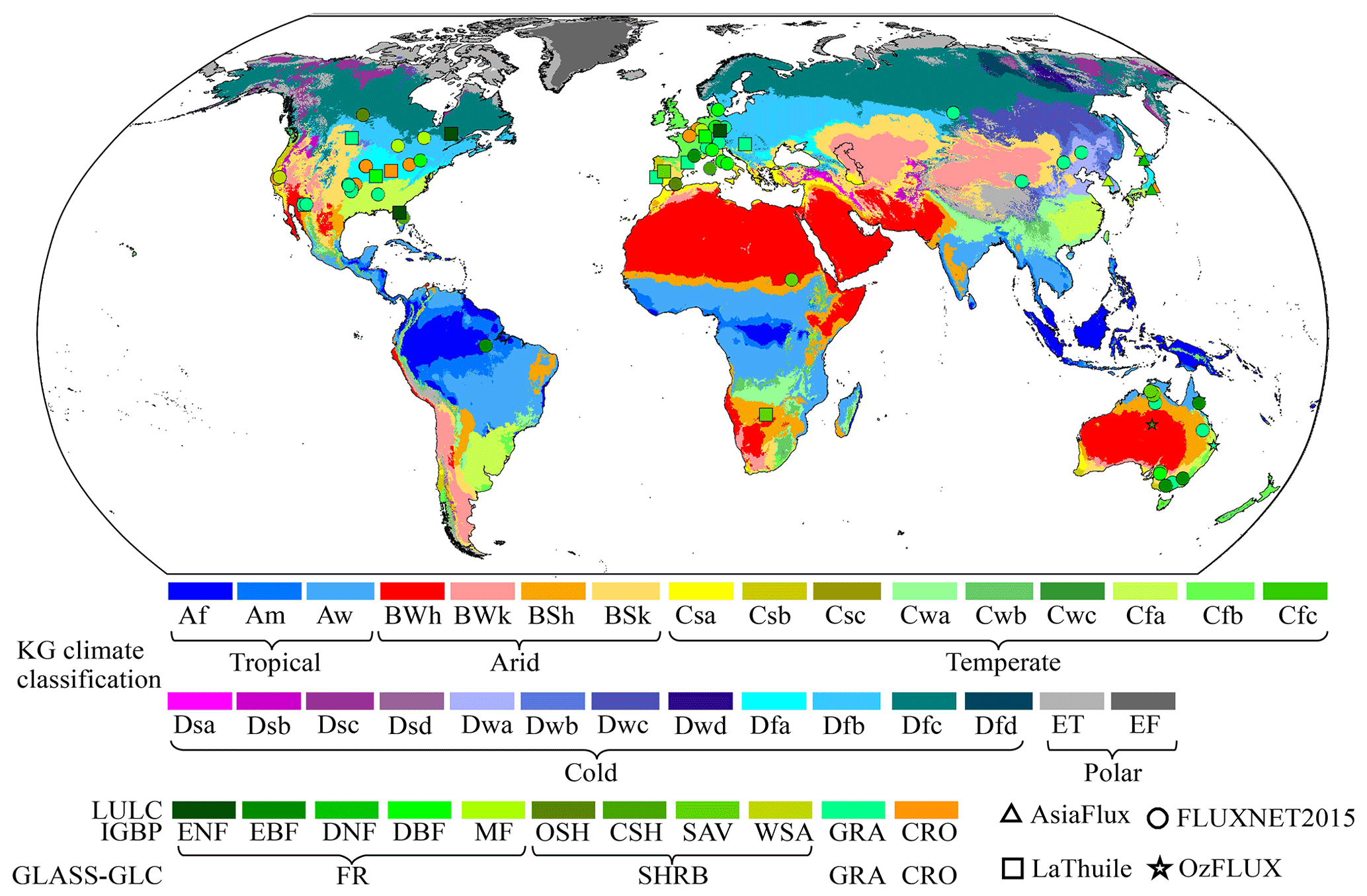
Figure 1 Locations of the used EC sites in this study over Köppen–Geiger (KG) climate regions (Beck et al., 2018). International Geosphere-Biosphere Programme (IGBP) classification system: CRO – cropland; GRA – grassland; DBF – deciduous broadleaf forest; EBF – evergreen broadleaf forest; ENF – evergreen needleleaf forest; MF – mixed forest; CSH – closed shrubland; WSA – woody savannah; SAV – savannah; OSH – open shrubland. GLASS-GLC classification system: FR – ENF, EBF, DNF, DBF, and MF; SHRB – SAV, CSH, OSH, and WSA; GRA; CRO.

2.1.2 Meteorological data

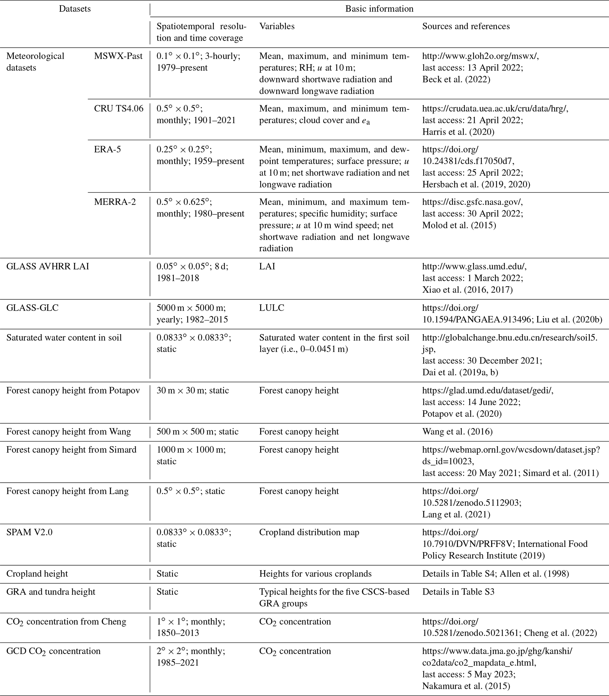
Meteorological inputs are necessary for generating the SW PET and, moreover, to reduce uncertainties, we collected four monthly or 3-hourly meteorological datasets, i.e., Multi-Source Weather (MSWX)-Past (Beck et al., 2022), National Aeronautics and Space Administration (NASA) Modern Era Reanalysis for Research and Applications (MERRA)-2 (Molod et al., 2015), European Centre for Medium-Range Weather Forecasts Reanalysis (ERA)-5 (Hersbach et al., 2020), and Climatic Research Unit (CRU) TS4.06 (Harris et al., 2020). The detailed information of these datasets is shown in Table 1. The directly used meteorological variables to drive the SW model mainly include air temperature, u, D, Rn, and G. Except for air temperature and u, the meteorological datasets provide different D-related and radiation-related variables (Table 1), and therefore different methods were utilized to estimate D and Rn (details in Supplement Sects. S1 and S2). Regarding G, the mean air-temperature-based method was used here (Allen et al., 1998; details in Supplement Sect. S3). Notably, because CRU TS4.06 lacked direct radiation records, the algorithm of Reddy (1974) was employed here to estimate Rn based on the Clouds and the Earth's Radiant Energy System (CERES) satellite-based monthly net shortwave radiation records (https://asdc.larc.nasa.gov/project/CERES, last access: 12 June 2022) and the CRU TS4.06 cloud cover data (algorithm and validation in Supplement Sect. S1 and Fig. S1, respectively). Moreover, due to no wind speed records in CRU TS4.06, we used the mean wind speed from the other three meteorological datasets as a proxy.

Table 1 Overview of major inputs for producing the global PET based on the calibrated SW model.

Note: due to unavailable minimum and maximum temperatures for the monthly ERA5 and MERRA-2 datasets, monthly values of the two variables were extracted from their hourly datasets.

2.1.3 Land use and land cover, LAI, saturated water content in soil, and CO₂ concentration

Considering the time span of the available LULC products at present, the 1982–2015 yearly GLASS-Global Land Cover (GLC) dataset developed by Liu et al. (2020a, b) at a spatial resolution of 5000 m was used here (Table 1), though it has a coarse LULC classification ecosystem (including cropland (CRO), forest (FR), grassland (GRA), shrubland (SHRB), tundra, barren land, and snow or ice). Some studies stated that the accuracy of the GLASS LAI is clearly better than that of others (e.g., the Moderate-resolution Imaging Spectroradiometer (MODIS) LAI), especially for forested areas with more realistic and reasonable trajectories representing seasonal variations (Fang et al., 2013; Liang et al., 2013; Xiao et al., 2014, 2016, 2017). Thus, the 1981–2018 8 d GLASS Advanced Very High Resolution Radiometer (AVHRR) LAI product at a spatial resolution of 0.5^∘ was selected in this study (Xiao et al., 2016, 2017; Table 1). The global saturated soil water content in the first soil layer (i.e., 0–0.0451 m) was collected from http://globalchange.bnu.edu.cn/research/soil5.jsp (last access: 30 December 2021​​​​​​​) (Dai et al., 2019a, b; Table 1), while the 1850–2013 monthly CO₂ concentration at 1^∘ × 1^∘ spatial resolution was downloaded from https://doi.org/10.5281/zenodo.5021361 (Cheng et al., 2022; Table 1). Because this CO₂ dataset missed the data in 2014 and 2015, the 1985–2021 monthly Global CO₂ Distribution (GCD) product from the Japan Meteorological Agency at a 2^∘ × 2^∘ spatial resolution (https://www.data.jma.go.jp/ghg/kanshi/co2data/co2_mapdata_e.html, last access: 5 July 2023; Maki et al., 2010; Nakamura et al., 2015; Table 1) was used to estimate the monthly CO₂ concentration in the 2 missing years by the linear regression method. In detail, we firstly resampled the GCD data into a 1^∘ × 1^∘ resolution and used the 1985–2013 GCD as an independent variable and Cheng's data as a dependent variable to fit the linear regressions for each month and each grid. Subsequently, based on the GCD data, these regressions were used to calculate the monthly CO₂ concentration on each grid in 2014 and 2015. The validation results of the established regression are in Fig. S2.

2.1.4 Vegetation canopy height

To date, the vegetation canopy height (h) maps to fully cover the whole globe are still lacking, although they are needed for the SW model to estimate some key parameters. Therefore, we made use of the existing datasets, mainly including the remote-sensing-based forest h datasets of Potapov et al. (2020), Wang et al. (2016), Simard et al. (2011), and Lang et al. (2021, 2022), respectively named h-Potapov, h-Wang, h-Simard, and h-Lang (Table 1), and the Spatial Production Allocation Model (SPAM) V2.0 crop distribution map (Yu et al., 2020; Table 1) to reconstruct the global vegetation h maps. For each year, the detailed procedures are four-fold. (1) Map FR and SHRB h. To reduce uncertainties related to the retrieval algorithms and source data, the h-Potapov, h-Wang, h-Simard, and h-Lang datasets were used in this procedure. Notably, we ignored differences in periods of source data for producing the forest h datasets. That is, we assumed that the changes in forest h due to vegetation natural growth were limited during the study period. To match GLASS-GLC, the four forest h datasets were firstly resampled to a spatial resolution of 5000 m. If two or more h datasets showed non-missing values at a certain FR (SHRB) grid cell, the average of these non-missing values represented the final h at this grid cell. After this, if some FR (SHRB) grid cells still had missing values, then the h value at each of these grid cells was filled with the mean h at the four nearest FR (SHRB) grid cells around this grid cell. (2) Map GRA and tundra h. Although the h-Lang product provided GRA and tundra h values over a few regions, there were still large areas with missing values, and even large uncertainties existed (Huang et al., 2017). Therefore, we specified the GRA and tundra h based mainly on the Comprehensive Sequential Classification System (CSCS)-based GRA groups and the typical GRA and tundra h measured at the EC sites and records from the literature. Using vegetation bioclimate characteristics and hydrothermal indictors (e.g., temperature and precipitation), the CSCS method was employed to classify the GLASS-GLC GRA and tundra into 10 groups (Li and Ma, 2009; Liang et al., 2011; Gang et al., 2016). According to the map of the CSCS-based GRA groups and the locations of the EC sites, the h value for each CSCS-based GRA group was estimated as the mean h from the EC sites with such a GRA group, and lastly the h values for seven CSCS-based GRA groups were determined. As for the remaining three CSCS-based GRA groups (i.e., frigid desert GRA, warm desert GRA, and tropical zonal forest steppe GRA), their h values were from White (1983), Suttie et al. (2005), Kadeba et al. (2015), Yin et al. (2019), and Prakash et al. (2020). The h values of all the CSCS-based GRA groups can be found in Table S3. (3) Map CRO h. By overlaying the SPAM V2.0 and GLASS-GLC maps, CRO was further classified into 42 types, and the h for each type was specified based on Table S4 (Allen et al., 1998). (4) Map the h of barren land and snow or ice. As for the barren land and snow or ice regions, the h was set to 0. Notably, regardless of the h map reconstructed for each year, this dataset could not reflect interannual variations of h except for regions with LULC changes, where the h values varied due to LULC changes. In the grid with LULC changes in a certain year, its new h value was assigned as the mean h value of its four nearest-neighbor grids with the same LULC. An example of the reconstructed canopy h map in 1982 is shown in Fig. S3.

2.2 Analysis methods

The workflow of this study mainly included three parts (Fig. 2): (1) calibrating the SW model based on the identified EC observations without water limits at 96 EC sites and validating its performance in site-calibration and cross-validation modes (cyan color in Fig. 2); (2) generating the global monthly PET using the calibrated SW model with the final minimum stomatal resistance (r_smin, s m⁻¹) values and various inputs (orange color in Fig. 2); and lastly (3) conducting related analyses, i.e., climatological characteristics and spatiotemporal changes in PET and its two components, together with climatological characteristics of PET partitioning (green color in Fig. 2).

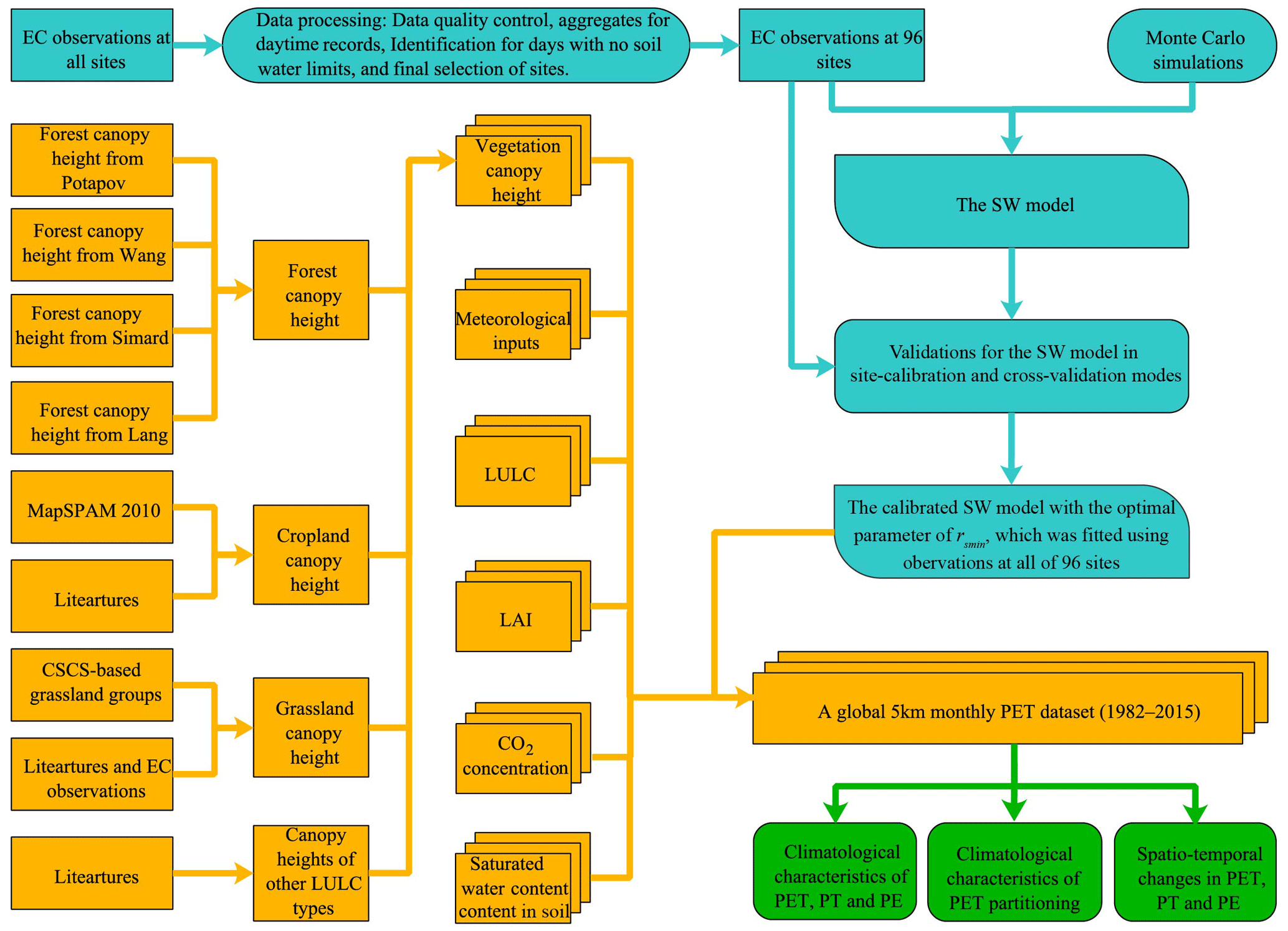
Figure 2 Workflow of this study. The blue and yellow-green colors show operating procedures for calibrating and validating the SW model and for producing a global 5 km monthly PET dataset, respectively, while the green color shows the related analyses.

2.2.1 Description of the SW model

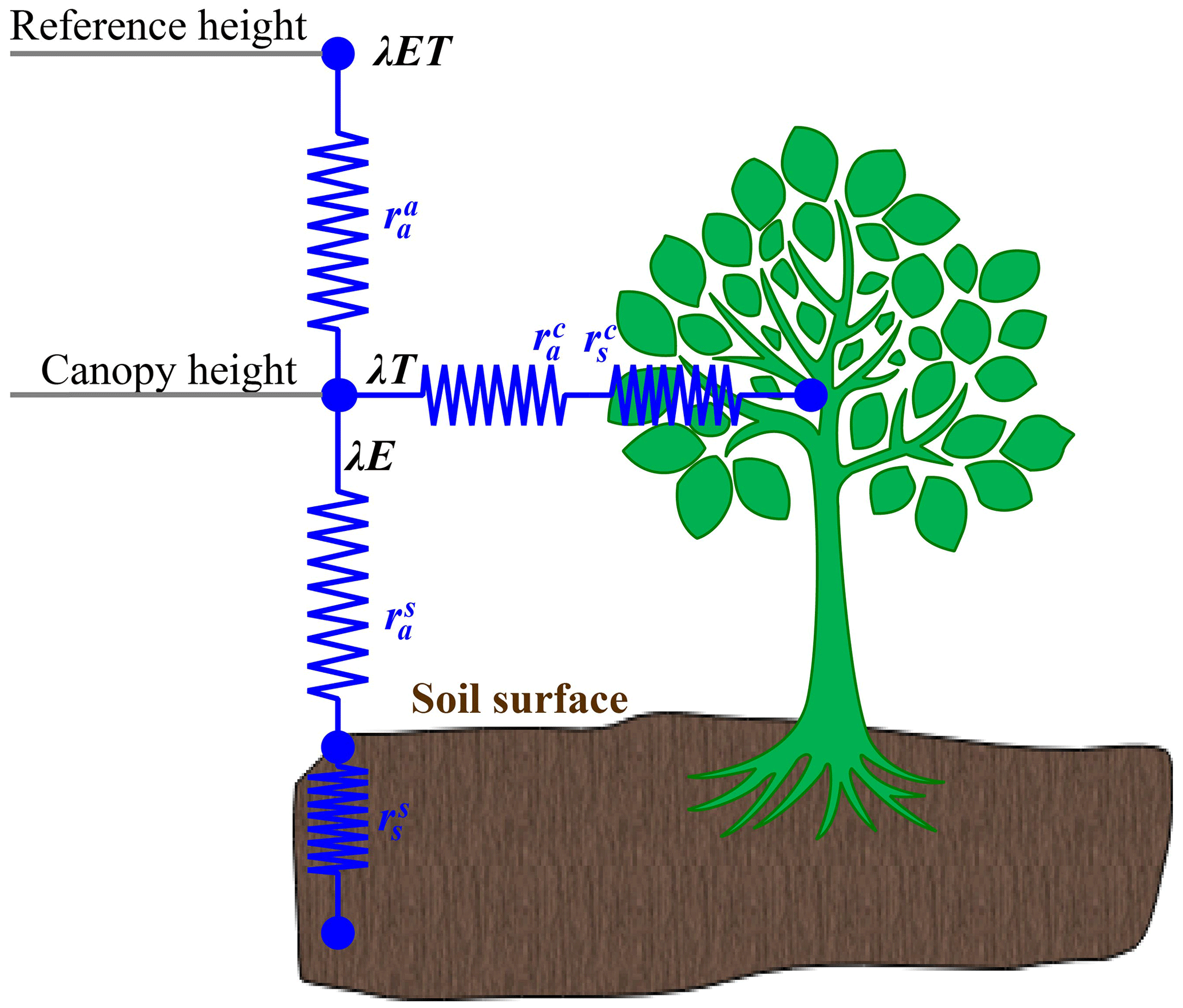
Based on the assumption that the water vapor arriving at the reference height is a mixture of evaporation from soil and transpiration from the vegetation layer (Fig. 3; Shuttleworth and Wallace, 1985; Wallace et al., 1990), the SW model can be expressed as

$$\textcolor{red}{}$$

where λET is the total latent heat flux (W m⁻²), i.e., the sum of the canopy (λT_r) and vegetation latent heat fluxes (λE), where T_r and E represent transpiration and soil evaporation, respectively; PM_c and PM_s are the closed vegetation and bare soil latent heat fluxes (W m⁻²), respectively, which can be calculated by the Penman formulas under conditions of bare soil (i.e., Eq. 1d) and closed canopy (i.e., Eq. 1e); C_c and C_s represent soil surface resistance (i.e., Eq. 1f; unitless) and canopy resistance coefficients (i.e., Eq. 1g; unitless), respectively; Δ denotes the slope of the saturated vapor pressure curve (kPa K⁻¹); γ is the humidity constant (kPa K⁻¹); λ is the latent heat of evaporation (MJ kg⁻¹); ρ is the air density (kg m⁻³); c_p is the constant pressure-specific heat (1013 J kg⁻¹ K⁻¹); $r_{\mathrm{a}}^{\mathrm{a}}$, $r_{\mathrm{a}}^{\mathrm{c}}$, and $r_{\mathrm{a}}^{\mathrm{s}}$ are the aerodynamic resistance (s m⁻¹), the vegetation boundary layer resistance (s m⁻¹), and the soil boundary layer resistance (s m⁻¹), respectively; and $r_{\mathrm{s}}^{\mathrm{s}}$ is the soil surface resistance, while $r_{\mathrm{s}}^{\mathrm{c}}$ is the vegetation canopy resistance (s m⁻¹). Based on Eq. (1b) (Eq. 1c), T_r (E) can be obtained with C_cPM_c (C_sPM_s) divided by λ.

Figure 3 Schematic description of the energy partitioning for a canopy with the SW model.

In Eq. (1b) and (1c), A and A_soil are the available energy for the canopy and soil layers (W m⁻²), respectively, and are defined as

$$\textcolor{red}{}$$

where R_n,soil is the net radiation fluxes into the soil (W m⁻²) and can be computed with Beer's law (i.e., Eq. 2c; Mo et al., 2004); k_ex represents the light extinction coefficient, which varies with the LULC types (Table S5).

Previous studies have stated that determining the five resistance parameters is the key to successfully running the SW model (Hu et al., 2009; Chen et al., 2022). Of these resistance parameters, $r_{\mathrm{a}}^{\mathrm{a}}$ and $r_{\mathrm{a}}^{\mathrm{s}}$ are estimated using Shuttleworth and Gurney (1990), while $r_{\mathrm{a}}^{\mathrm{c}}$ and $r_{\mathrm{s}}^{\mathrm{s}}$ are calculated based on Shuttleworth and Wallace (1985), Brisson et al. (1998), and Villagarcía et al. (2010), respectively. Detailed information about equations for parameterizing the four resistance parameters can be found in Supplement Sects. S4–S6 and Table S5. Considering large uncertainties of $r_{\mathrm{s}}^{\mathrm{c}}$ (Fisher et al., 2005; Hu et al., 2009, 2013; Wei et al., 2020), this study used the EC measurements to calibrate its value for each LULC type, and the detailed procedures can be found in Sect. 2.2.2.

2.2.2 Determination of canopy resistance ($r_{\mathrm{s}}^{\mathrm{c}}$)

In this study, the parameterization of $r_{\mathrm{s}}^{\mathrm{c}}$ is mainly based on a Jarvis-type model, which is based on the hypothesis that stomatal resistance is independently affected by every environmental variable (Jarvis, 1976; Shuttleworth and Wallace, 1985). Here, we considered effects of the LAI, D, air temperature (T, ^∘C), soil moisture, and ${\mathit{\rho }}_{{\mathrm{CO}}_{\mathrm{2}}}$ on $r_{\mathrm{s}}^{\mathrm{c}}$, which correspond to stress functions of F₁ (Noilhan and Planton, 1989), F₂ (Raab et al., 2015), F₃ (Zhou et al., 2006), F₄, and F₅ (Neitsch et al., 2002). Notably, this study focuses on ET under a condition with no soil water limits (namely PET), and thus F₄ is set to 1 here. The specific equations are shown as follows:

$$\textcolor{red}{}$$

where r_smax is the maximum canopy resistance (s m⁻¹) and is fixed at 5000 s m⁻¹ here (Crow and Kustas, 2008); LAIe denotes the effective LAI (Gardiol et al., 2003); R_ds is the downward shortwave radiation (W m⁻²); R_ds,dbl is the minimum shortwave radiation threshold for vegetation to carry out photosynthesis (W m⁻²), which is set to 30 W m⁻² for forests and 100 W m⁻² for other vegetation (Noilhan and Planton, 1989; Lo Seen et al., 1997); and $\mathrm{\Delta }{g}_{\mathrm{1},{\mathrm{CO}}_{\mathrm{2}}}$ is the multiple of leaf stomatal conductance reduction when ${\mathit{\rho }}_{{\mathrm{CO}}_{\mathrm{2}}}$ is doubled (Table S5; Morison and Gifford, 1984; Field et al., 1995; Saxe et al., 1998; Neitsch et al., 2002; Eckhardt and Ulbrich, 2003; Wu et al., 2017).

Finally, we determined the values of r_smin. Here, the Monte Carlo method was used to calibrate this parameter using the identified PET observations at each EC site (Hu et al., 2009). The following five steps were taken to determine the r_smin values: (1) giving a rough range for r_smin (i.e., r_smin between 1 and 500 s m⁻¹) with reference to previous studies (e.g., Zhou et al., 2006; ECWMF, 2007); (2) conducting 5000 Monte Carlo simulations with the parameter sets randomly sampled from uniform distributions within the given ranges; (3) comparing the estimated SW model-based PET (SW PET) and the EC PET after each simulation based on a validation metric of the Kling–Gupta efficiency (KGE; see Eq. 4d; Gupta et al., 2012; 5000 parameter sets corresponded to 5000 KGEs after this step); (4) selecting the mean of r_smin with the 10 highest KGEs as the optimal value for each site; and (5) classifying the 96 EC sites into four types (i.e., FR, SHRB, CRO, and GRA) based on the GLASS-GLC classification system (Liu et al., 2020a, b) and then determining the best-fit parameter sets for a given LULC type by averaging the optimal parameter values at the sites with this LULC type. In this way, the final parameter values for FR, CRO, GRA, and SHRB were obtained and are illustrated in Table S6. Notably, the r_smin for the tundra, barren land, and snow or ice types of GLASS-GLC are from Zhou et al. (2006) and Zhang et al. (2008), mainly due to the lack of the corresponding EC observations.

2.2.3 Model validation

Several validation metrics were employed to evaluate the performance of the simulated SW PET. Mean error (ME) provides a way of quantifying the biases of the estimates relative to the measurements, while root-mean-square error (RMSE) describes the accuracy of the estimations. In addition, the correlation coefficient (R) and KGE (with a range between −∞ and 1.0, the optimal value) were used to measure the capability of capturing the spatiotemporal variability and the overall performance of the SW PET, respectively. The metrics are expressed as

$$\textcolor{red}{}$$

where N is the sample number; S denotes the mean of the SW-PET-averaged N samples; O is for the measured PET; i is the ith sample; α is $S/O$; and β is ${\mathit{\sigma }}_S/{\mathit{\sigma }}_O$, where σ_S and σ_O are the standard deviations of the estimated and measured PET, respectively.

These metrics were first computed based on the daily estimates with the optimal parameters for each site, i.e., parameters obtained in step (4) of the Monte Carlo method, and the observations from the 96 EC sites, and then validation in site-calibration mode was performed. Notably, to evaluate the transferability of the calibrated parameters from known observations to any location and then the robustness of the established SW model, the “leave-one-out” cross-validation method was utilized here (Zhang et al., 2019). For each LULC type, the data from one “ungauged” observation were excluded from the Monte Carlo method-based optimization, while the data from all other observations of the same LULC type were used for model calibration to obtain the simulated one in the ungauged position. All four LULC types were actualized in this way. Then, the daily SW PET estimates in cross-validation mode were compared against the daily observations from the 96 EC sites to further explore the model performance.

2.2.4 Development of the 5 km global monthly PET (1982–2015) and related analyses

Considering that the SW model was calibrated with the daily EC measurements, it was necessary to examine whether this model could be applicable at the monthly scale. Therefore, we firstly compared the monthly PET estimated based on the daily and monthly meteorological variables from MSWX-Past, MERRA-2, and ERA-5 (not including CRU TS4.06, mainly due to it being at a monthly scale). Various validation metrics showed that there were generally no evident differences in the two PET estimates (Fig. S4). That is, the model established with the daily EC measurements could be driven using the monthly meteorological variables. Mainly due to GLASS-GLC having the shortest time span, the global SW PET was produced at the GLASS-GLC grid and monthly scale during 1982–2015. Therefore, before running the calibrated SW model, the meteorological, GLASS LAI, and CO₂ concentration datasets were resampled to a spatial resolution of 5000 m. The monthly mean meteorological and LAI datasets were taken as inputs to run the calibrated model for estimating the monthly mean SW PET, PT, and PE. Finally, the total SW PET values (PT and PE) of a certain month were obtained by the monthly mean value multiplied by the days of this month. Additionally, to reduce uncertainties from the meteorological datasets, the ensemble means of PET, PT, and PE based on the four meteorological datasets were provided. Using the ensemble mean PET, PT, and PE, we analyzed climatological characteristics and spatiotemporal changes in PET and its two components together with climatological characteristics of PET partitioning. Notably, the area-weighted method was used to estimate the regional mean PET, PT, and PE.

3 Results

3.1 Performance of the established SW model

The simulated daily PET from the SW model was first evaluated against EC measurements aggregated for all 96 EC sites (Fig. 4a and c). In both the site-calibration and cross-validation modes, the SW model could simulate the daily PET well, with most of the data points around the 1:1 line, while it should be noted that overestimation and underestimation existed for the lower and higher measurements, respectively (Fig. 4a). Based on the selected validation metrics, we could conclude that the model had excellent performance in the two modes, with R, ME, RMSE, and KGE values above 0.85, between −0.03 and −0.01 mm d⁻¹, below 0.80 mm d⁻¹, and above 0.85, receptively. Regarding the mean values of each site (Fig. 4b and d), the simulated daily PET could also follow well changes in the observed PET among the 96 sites in both modes, as evidenced by R above 0.88, ME between −0.09 and −0.03 mm d⁻¹, RMSE below 0.60 mm d⁻¹, and KGE above 0.85. Moreover, little changes in the validation metrics from site calibration to cross-validation indicated limited degradation of the calibrated model (i.e., Fig. 4a vs. 4c and Fig. 4b vs. 4d).

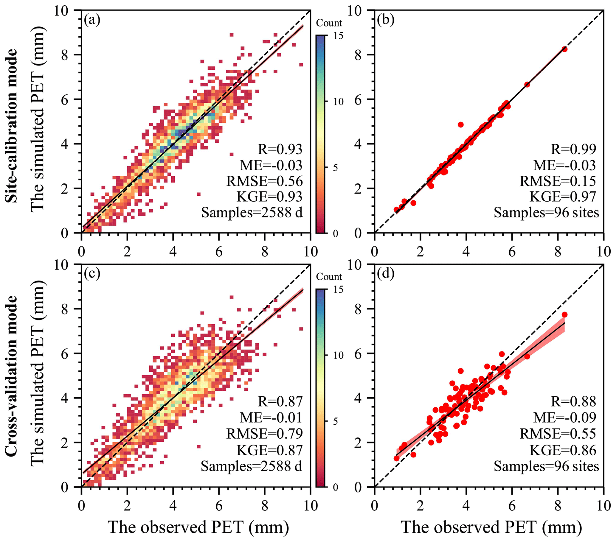
Figure 4 Scatterplots of observations against simulations aggregated for all of the 96 EC sites. (a) Daily comparison in site-calibration mode. (b) Site mean comparison in site-calibration mode. (c) Daily comparison in cross-validation mode. (d) Site mean comparison in cross-validation mode. In these figures, the dashed and solid lines are the 1:1 line and the regression line with the least-square method, while the shadow area represents the 95 % confidence interval.

Figure 5 indicates that, in site-calibration and cross-validation modes, the SW model estimated daily PET very well for FR, SHRB, GRA, and CRO. The model slightly overestimated lower daily PET but slightly underestimated higher daily PET. The performance of this model differed slightly among LULC types. R was above 0.83, indicating that the model could successfully simulate the spatiotemporal variability of the daily PET, especially for FR, SHRB, and GRA in site-calibration mode. Although negative and positive ME existed in CRO and GRA and the other two LULC types, respectively, the ME magnitudes were all below 0.15 mm. According to RMSE, the simulated GRA daily PET performed best in each mode, while larger values (between 0.54 and 0.85 mm d⁻¹) occurred in the other three LULC types, especially for CRO in site-calibration mode and FR in cross-validation mode. The KGE was always larger than 0.80 for each LULC type in site-calibration and cross-validation modes, which indicated that the calibrated model overall had a high performance. When it came to validation based on site mean values (Fig. 6), the simulated PET followed changes in the observed PET for each LUCC type well in the two modes, with R above 0.74, ME between −0.12 and 0.11 mm, RMSE below 0.70 mm, and KGE above 0.74. For each LULC type, the cross-validation mode had a slightly lower performance than the site-calibration mode (Fig. 6a vs. 6e, Fig. 6b vs. 6f, Fig. 6c vs. 6g, and Fig. 6d vs. 6h).

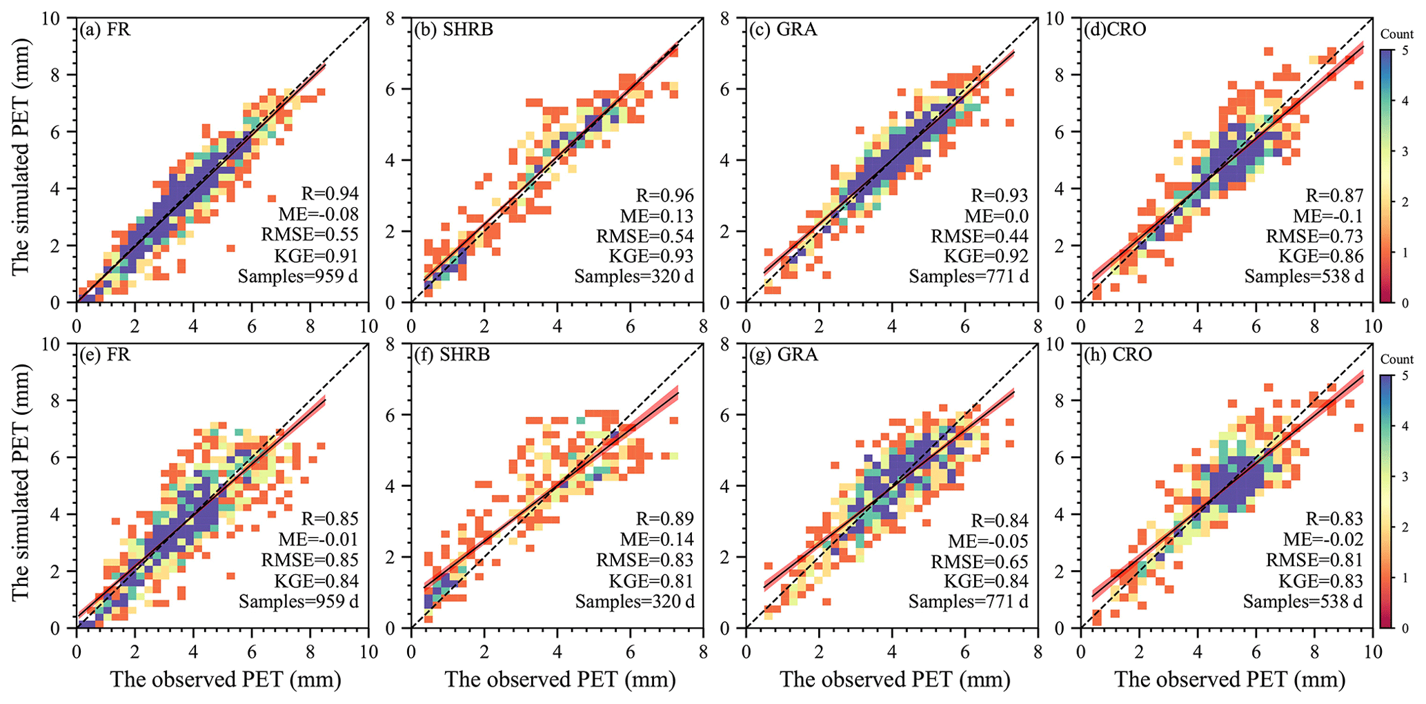
Figure 5 Scatterplots of daily observations against simulations aggregated for the different LULC types. (a–d) Comparison in site-calibration mode. (e–h) Comparison in cross-validation mode. In these figures, the dashed and solid lines are the 1:1 line and the regression line with the least-square method, while the shadow area represents the 95 % confidence interval.

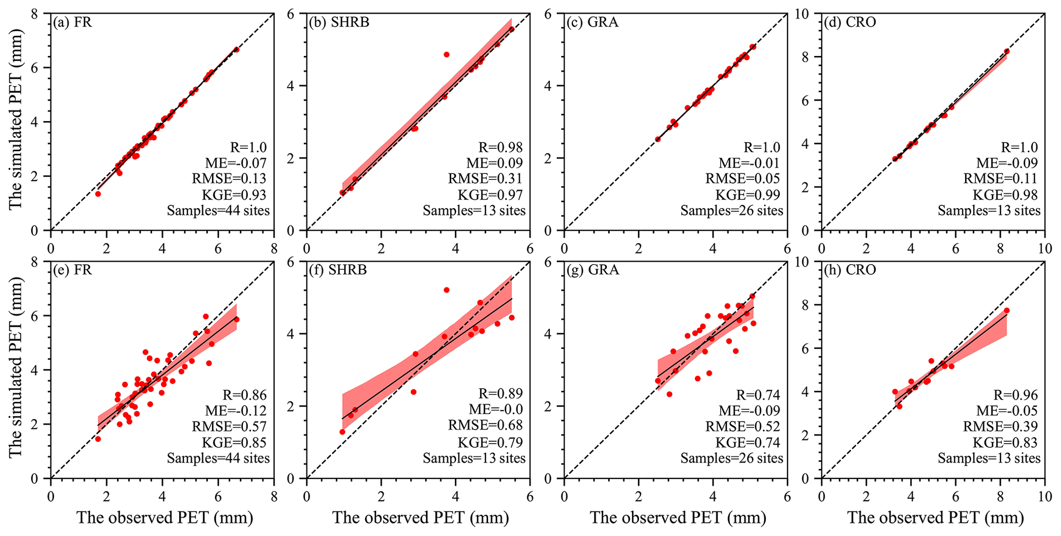
Figure 6 Scatterplots of site mean observations against simulations for each LULC type. (a–d) Comparison in site-calibration mode. (e–h) Comparison in cross-validation mode. In these figures, the dashed and solid lines are the 1:1 line and the regression line with the least-square method, while the shadow area represents the 95 % confidence interval.

To further evaluate the performance of the established SW model, we also computed the validation metrics at each site for each LULC type in site-calibration and cross-validation modes, which are shown in Fig. 7. Except for several sites for SHRB, GRA, and CRO, the R values were all above 0.80, and more than 50 % of the sites had a value above or around 0.90, which indicated that the model had excellent performance in capturing the temporal variability of daily PET (Fig. 7a). As for ME, the majority of the sites for each LULC type showed a range between −0.50 and 0.50 mm (Fig. 7b). Moreover, the daily PET for SHRB (the other three LULC types) was overestimated (underestimated) by the SW model at more than 50 % of the sites. Except for a few sites, the RMSE values were below 0.80 mm at more than 75 % of the sites for each LULC type, and comparably the RMSE-based performance for CRO was the worst generally, with an RMSE above 0.50 mm (Fig. 7c). The majority of the sites had a KGE value above 0.60 and, especially for GRA and CRO, more than 75 % of the sites had a KGE larger than 0.70 (Fig. 7d). In general, the model performance in cross-validation mode was similar to or only slightly lower than that in the calibration model for each LULC type.

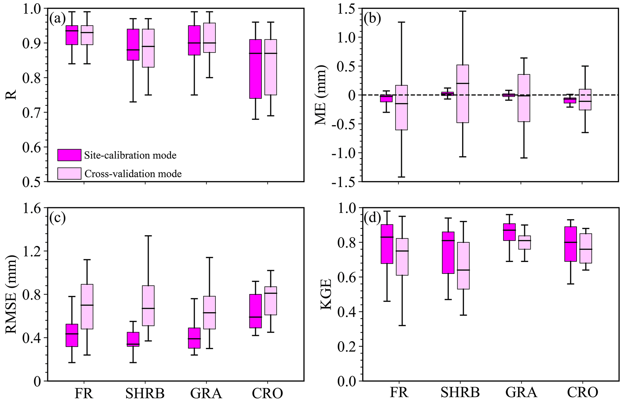
Figure 7 Boxplots of the validation metrics of daily PET simulations for each LULC type. The whiskers represent the minimum and maximum values of the model performance metrics. The outer edges of the boxes and the horizontal lines within the boxes indicate the 25th, 75th, and 50th percentiles of the validation metrics.

To sum up, the above evaluation indicated that the calibrated parameter of r_smin could be transferable from known observations to any location, and then the established SW model could simulate PET well across different LULC types. This gave us the confidence to employ it in producing a global PET dataset. Notably, to maximize data utilization, the final values of r_smin for each LULC type were determined based on all the EC observations (Table S6), and the related validation results can be found in Fig. S5.

3.2 Climatological characteristics of PET, PT, and PE

As seen from Fig. 8a, c, and e, the global mean climatological annual PET, PT, and PE were 1198.96, 481.12, and 717.74 mm, respectively. Compared to the Northern Hemisphere (NH), a larger mean climatological annual PT and thus PET appeared in the Southern Hemisphere (SH), where a larger proportion of the land surface was covered by vegetation. Among the five KG climate regions, mean climatological annual values of PET and its two components showed evident differences, with a range from 319.29 mm in the “Polar” region to 1590.57 mm in the “Tropical” region for PET, from 37.95 mm in the Polar region to 1122.42 mm in the Tropical region for PT, and from 248.31 mm in the “Cold” region to 1379.16 mm in the “Arid” region for PE. Except for the Tibetan Plateau with a lower value, climatological annual PET was generally larger than 1000 mm between 60^∘ S and 45^∘ N, covering 62 % of the globe (Fig. 8b). In particular, climatological annual PET exceeded 1800 mm over northern Africa, the Arabian Peninsula, the Indian Peninsula, the Indo-China Peninsula, and northern Australia. The lowest climatological annual PET (<400 mm) was generally located to the north of 60^∘ N. As seen in Fig. 8d, the spatial distribution of climatological annual PT differed from that of climatological annual PET. Due to sparse and even no vegetation and/or unfavorable climate conditions, lower climatological annual PT (<400 mm) was widely distributed to the north of 18^∘ N and to the south of 18^∘ S, corresponding to an area percentage of 55 %. By contrast, 16 % of the globe with larger climatological annual PT (>1200 mm) was mainly located in the Caribbean, the Amazon Basin, the Congo Basin, and the Indo-China Peninsula. As for climatological annual PE (Fig. 8f), larger values (>1000 mm) were generally clustered in northwestern North America and South America, northern Africa, western Asia, and most of Australia, which corresponded to sparse and even no vegetation and covered 36 % of the globe. Notably, lower climatological annual PE (<400 mm) appeared in tropical rainforests near the Equator, possibly because the dense vegetation limited the available energy for PE.

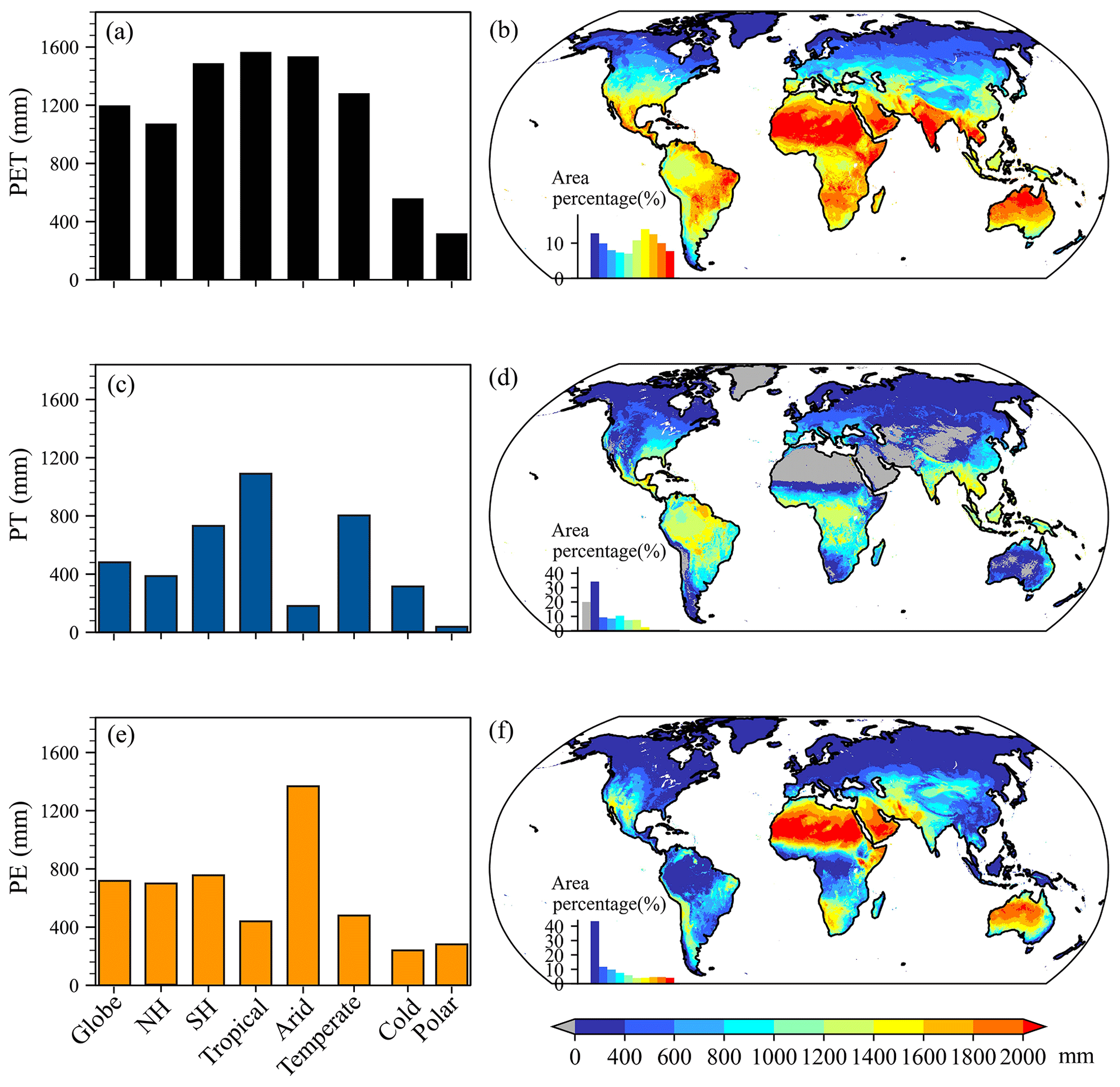
Figure 8 Climatological annual PET, PE, and PT. (a) Climatological annual PET averaged over the globe, the Northern Hemisphere (NH) and Southern Hemisphere (SH), and each KG climate region. (b) Spatial distribution of climatological annual PET. (c) Climatological annual PT averaged over the globe, NH and SH, and each KG climate region. (d) Spatial distribution of climatological annual PT. (e) Climatological annual PE averaged over the globe, NH and SH, and each KG climate region. (f) Spatial distribution of climatological annual PE. In panels (b), (d), and (f), the inset histogram shows the area percentage stratified by the amount of annual PET, PT, or PE.

As expected, climatological monthly PET, PT, and PE generally exhibited strong seasonal fluctuations because of the combined influences from many environmental factors (Fig. 9). The globe and the NH showed similar seasonal cycles for climatological monthly PET, PT, and PE, i.e., increasing from January, peaking in July, and declining afterwards, while an opposite seasonal fluctuation existed in the SH, with a valley in June (Fig. 9a–c). Mainly due to differences in environmental factors, the seasonal cycles of climatological monthly PET, PE, and PT obviously differed among various KG climate regions (Fig. 9d–h). As for the Tropical region, no evident seasonal fluctuations existed for the three variables, which slightly fluctuated around 136 mm for monthly PET, 88 mm for monthly PT, and 40 mm for monthly PE, respectively (Fig. 9d). In the Arid, Cold, and Polar regions, climatological monthly PE, PT, and PE were generally characterized by a peak in July or August (Fig. 9e, g, and h), while the Temperate region showed larger values in April–November (Fig. 9f).

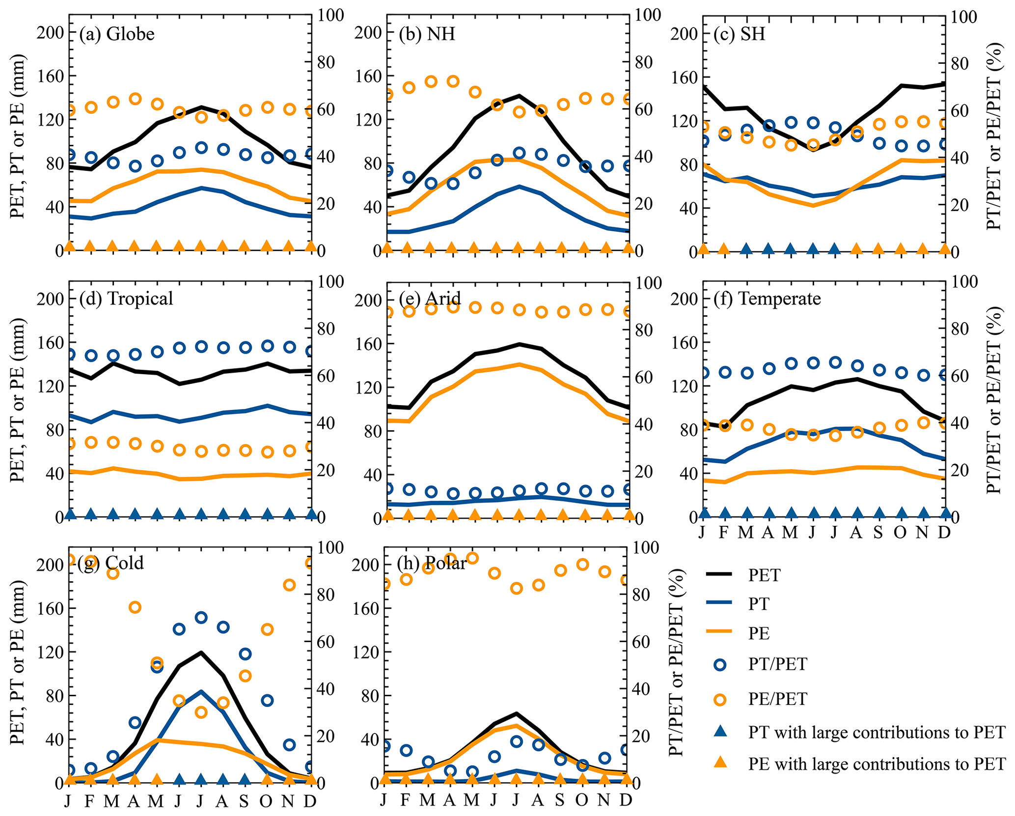
Figure 9 Climatological monthly PET, PE, PT, $\mathrm{PE}/\mathrm{PET}$, and $\mathrm{PT}/\mathrm{PET}$ averaged over the globe, each hemisphere, and each KG climate region.

3.3 Climatological characteristics of PET partitioning

In order to know PET partitioning, we estimated the ratios of PT and PE to PET (i.e., $\mathrm{PT}/\mathrm{PET}$ and $\mathrm{PE}/\mathrm{PT}$) at annual and monthly scales (Figs. 9 and 10). As depicted in Fig. 10a and c, the global mean annual $\mathrm{PT}/\mathrm{PET}$ and $\mathrm{PE}/\mathrm{PET}$ were 41 % and 59 %, respectively, indicating that globally the annual PE greatly contributed to the annual PET. Likewise, the annual PE was also a major contributor in the NH and SH, with $\mathrm{PE}/\mathrm{PET}$ values of 62 % and 50 %, respectively. Overall, the annual $\mathrm{PT}/\mathrm{PET}$ ($\mathrm{PE}/\mathrm{PET}$) had evident regional differences and was above 53 % (below 47 %) in the Tropical, Temperate, and Cold regions but below 12 % (above 88 %) in the other two climate regions (Fig. 10a and c). These indicated that the annual PET in the Tropical, Temperate, and Cold regions (Arid and Polar regions) was controlled by PT (PE). Spatially, the annual $\mathrm{PE}/\mathrm{PET}$ was above 50 %, mainly in regions to the north of 65^∘ N, western North America, Patagonia and the Andes of South America, western and central Asia, northern and southern Africa, and Australia (Fig. 10d), while the remaining regions showed a $\mathrm{PT}/\mathrm{PET}$ larger than 50 %, especially for the Amazon Basin, the Congo Basin, and Southeast Asia, with a value exceeding 90 %. Compared to the annual $\mathrm{PT}/\mathrm{PET}$, the annual $\mathrm{PE}/\mathrm{PET}$ corresponded to an opposite spatial distribution (Fig. 10b). In short, the annual PET was dominated by PE and PT over 59 % and 41 %, respectively, of the globe.

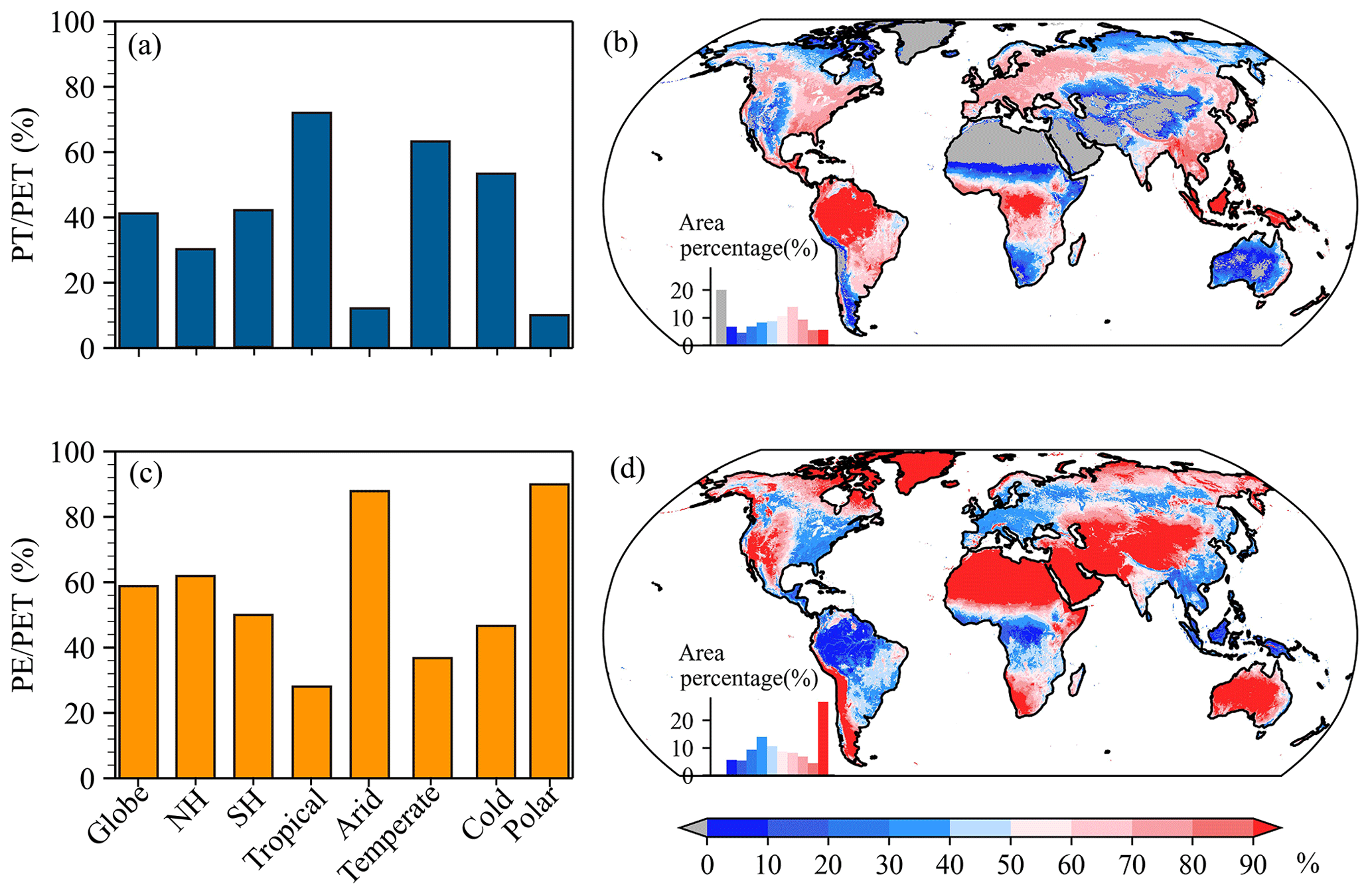
Figure 10 Characteristics of annual $\mathrm{PT}/\mathrm{PET}$ and $\mathrm{PE}/\mathrm{PET}$. (a) Annual $\mathrm{PT}/\mathrm{PET}$ averaged over the globe, each hemisphere, and each KG climate region. (b) Spatial distribution of annual $\mathrm{PT}/\mathrm{PET}$. (c) Annual $\mathrm{PE}/\mathrm{PET}$ averaged over the globe, each hemisphere, and each KG climate region. (d) Spatial distribution of annual $\mathrm{PE}/\mathrm{PET}$. In panels (b) and (d), the inset histogram shows the area percentage stratified by the amount of annual $\mathrm{PT}/\mathrm{PET}$ or $\mathrm{PE}/\mathrm{PET}$.

In general, the seasonal cycle of $\mathrm{PT}/\mathrm{PET}$ ($\mathrm{PE}/\mathrm{PET}$) for the globe, each hemisphere, and each KG climate region was different from that of PT (PE; Fig. 9). As for the global, NH, and Polar regions (Fig. 9a, b, and h), the monthly $\mathrm{PT}/\mathrm{PET}$ had two bottoms in April and October and a peak in July, corresponding to tow peaks and a bottom of the monthly $\mathrm{PE}/\mathrm{PET}$. In the SH and Temperate regions (Cold region), the monthly $\mathrm{PT}/\mathrm{PET}$ first increased from January, peaked in July (June), and declined after that, while the monthly $\mathrm{PE}/\mathrm{PET}$ showed the opposite fluctuations (Fig. 9c, f, and g). No evident fluctuations of the monthly $\mathrm{PT}/\mathrm{PET}$ and $\mathrm{PE}/\mathrm{PET}$ existed in the Tropical and Arid regions (Fig. 9d and e). Comparing the monthly $\mathrm{PT}/\mathrm{PET}$ and $\mathrm{PE}/\mathrm{PET}$ for the globe, NH, Arid region, and Polar region (Fig. 9a, b, e, and h), it was not difficult to find that the former was always smaller than the latter, indicating that the monthly PE greatly contributed to the monthly PET. By contrast, the larger monthly $\mathrm{PT}/\mathrm{PET}$ in the Tropical and Temperate regions suggested that PT dominated PET in these regions (Fig. 9d and f). In particular, the major contributor to the monthly PET for the SH (Cold region) varied throughout the year, i.e., PT dominating PET in March–July (May–September) but PE dominating PET in the other months (Fig. 9c and g).

3.4 Spatiotemporal changes in PET, PT, and PE

Globally, annual PET and PT significantly (p<0.05) increased by 1.26 and 1.27 mm yr⁻¹, respectively, with a slight and insignificant decrease in annual PE (Fig. 11a, c, and e). Regarding annual PET and PT, both the NH and the SH had significant (p<0.05) increases, while annual PE oppositely changed in the two hemispheres, i.e., increases for the NH but decreases for the SH (Fig. 11b and c). Among the various KG climate regions, annual PET (except for the Tropical region) and PT were all found to significantly (p<0.05) increase but with evident regional differences in magnitudes, i.e., larger PET increases (>1.32 mm yr⁻¹) in the Arid, Temperate, and Cold regions and a maximum increase (1.83 mm yr⁻¹) in PT in the Temperate region (Fig. 11a, c, and e). Except for the Polar region, the other climate regions all showed significant (p<0.05) changes in annual PE, followed by decreases in the Tropical and Temperate regions but increases in the Arid and Cold regions. Comparisons between annual trends of PT and PE suggested that the increases in PET could be attributed to increased PT for the globe, each hemisphere, and each climate region. Spatially, increases in annual PET covered 78 % of the globe, accompanied by 41 % of the globe, with significant (p<0.05) increases and larger values (>4.00 mm yr⁻¹) in the western US, the Amazon Basin, the Congo Basin, eastern Europe, and eastern China (excluding the northeastern part; Fig. 11b). As for annual PET, only 5 % of the globe had significant (p<0.05) reductions. Not considering non-vegetation regions, the spatial pattern of annual PT trends was similar to that of annual PET trends (Fig. 11d). Overall, significant (p<0.05) increases and decreases in annual PT were observed for 28 % and 4 %, respectively, of the globe, especially for the Amazon Basin, the Congo Basin, southern Africa, the Indian Peninsula, eastern Europe, and eastern China (excluding the northeastern part), with larger increases exceeding 4.00 mm yr⁻¹. As shown in Fig. 11f, the increasing trends of annual PE had a wide distribution, but significant (p<0.05) increases only covered over 26 % of the globe, and the increases were generally below 3.00 mm yr⁻¹. Relative to annual PET and PT, annual PE had more regions showing decreases, with significant (p<0.05) reductions over 17 % of the globe, mainly in northern South America, Australia, southern Africa, and the Indian Peninsula. In general, the spatial distribution of major contributors to annual PET trends was similar to that of major contributors to annual PET (Fig. 11g vs. Fig. 10b and d). For example, the major contributor of PE was mainly located in Greenland, southwestern North America, Patagonia and the Andes of South America, western and central Asia, northern and southern Africa, and most of Australia (Fig. 11g). By contrast, the remaining regions showed the dominant factor of PT. Overall, the annual PET changes were dominated by PT and PE over 53 % and 47 %, respectively, of the globe.

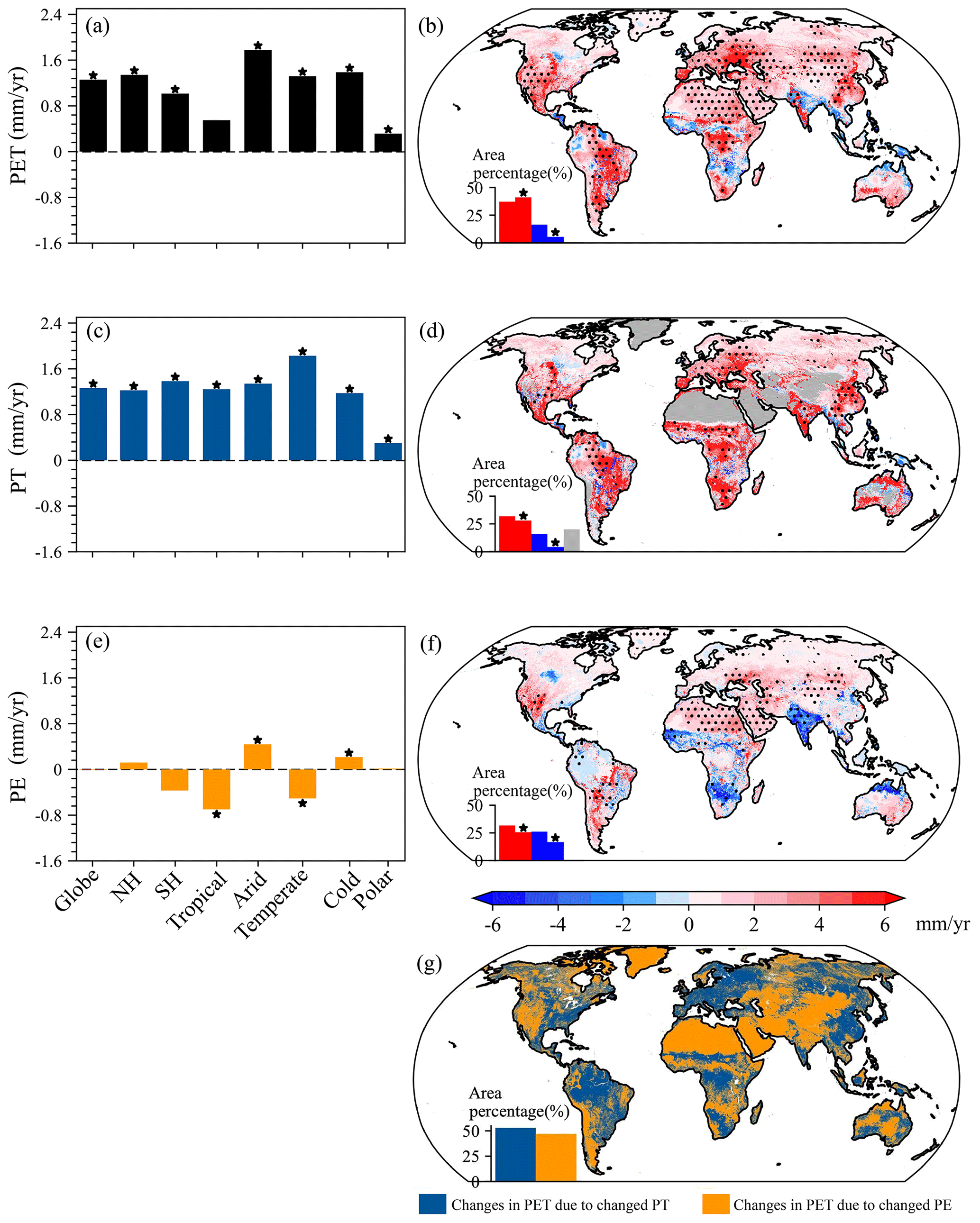
Figure 11 Characteristics of annual PET, PT, and PE trends together with major contributors to annual PET trends. (a) Trends for annual PET averaged over the globe, each hemisphere, and each KG climate region. (b) Spatial distribution of annual PET trends. (c) Trends for annual PT averaged over the globe, each hemisphere, and each KG climate region. (d) Spatial distribution of annual PT trends. (e) Trends for annual PE averaged over the globe, each hemisphere, and each KG climate region. (f) Spatial distribution of annual PE trends. (g) Spatial distribution of major contributors to annual PET trends. In panels (a), (c), and (e), the star indicates that the trend is significant (p<0.05). In panels (b), (d), and (f), the inset histogram suggests an area percentage of insignificant increases (red bar without a star), significant increases (red bar with a star; p<0.05), insignificant decreases (blue bar without a star), and significant decreases (blue bar with a star; p<0.05).

In general, the global mean monthly PET and PT significantly (p<0.05) increased throughout a year with larger trends (>0.10 mm yr⁻¹) during April–October, while the global mean monthly PE insignificantly changed in each month (Fig. 12a). For the NH (Figs. 12b), all months showed significant (p<0.05) increases in PET and PT, especially for March–September with trends generally larger than 0.10 mm yr⁻¹. Despite most of the months having increased PE, only March had significant (p<0.05) increases in the NH. In the SH (Fig. 12c), monthly PET showed larger (>0.10 mm yr⁻¹) and significant (p<0.05) increases during June–October but generally decreases in the other months. The SH PT significantly (p<0.05) increased in most of the months, with larger values (>0.12 mm yr⁻¹) during August–October. As for the SH PE, August and October (January–March and December) corresponded to significant (p<0.05) increases (reductions). Among the five KG climate regions (Fig. 12d–h), the monthly PET and PT increased throughout a year except for the PET of the Tropical region in several months with decreases, and moreover the increases in most of the months were significant (p<0.05). When it came to the monthly PE changes, most of or all of the months exhibited decreases in the Tropical and Temperate regions but generally increases in the other three KG climate regions. Despite that, no more than 6 months exhibited significant (p<0.05) increases or decreases in the monthly PE for each climate region. Furthermore, we compared trends of the monthly PT and PE to identify major contributors to the monthly PET changes in the globe, each hemisphere, and each KG climate region (Fig. 12). Overall, the monthly PET changes were generally dominated by PT in most of or all of the months for the globe and each region. However, it should be noted that PE was the major contributor of PET for some months, i.e., January–March for the SH, February–May for the Tropical region, March and December for the Cold region, and February–May, October, and November for the Polar region.

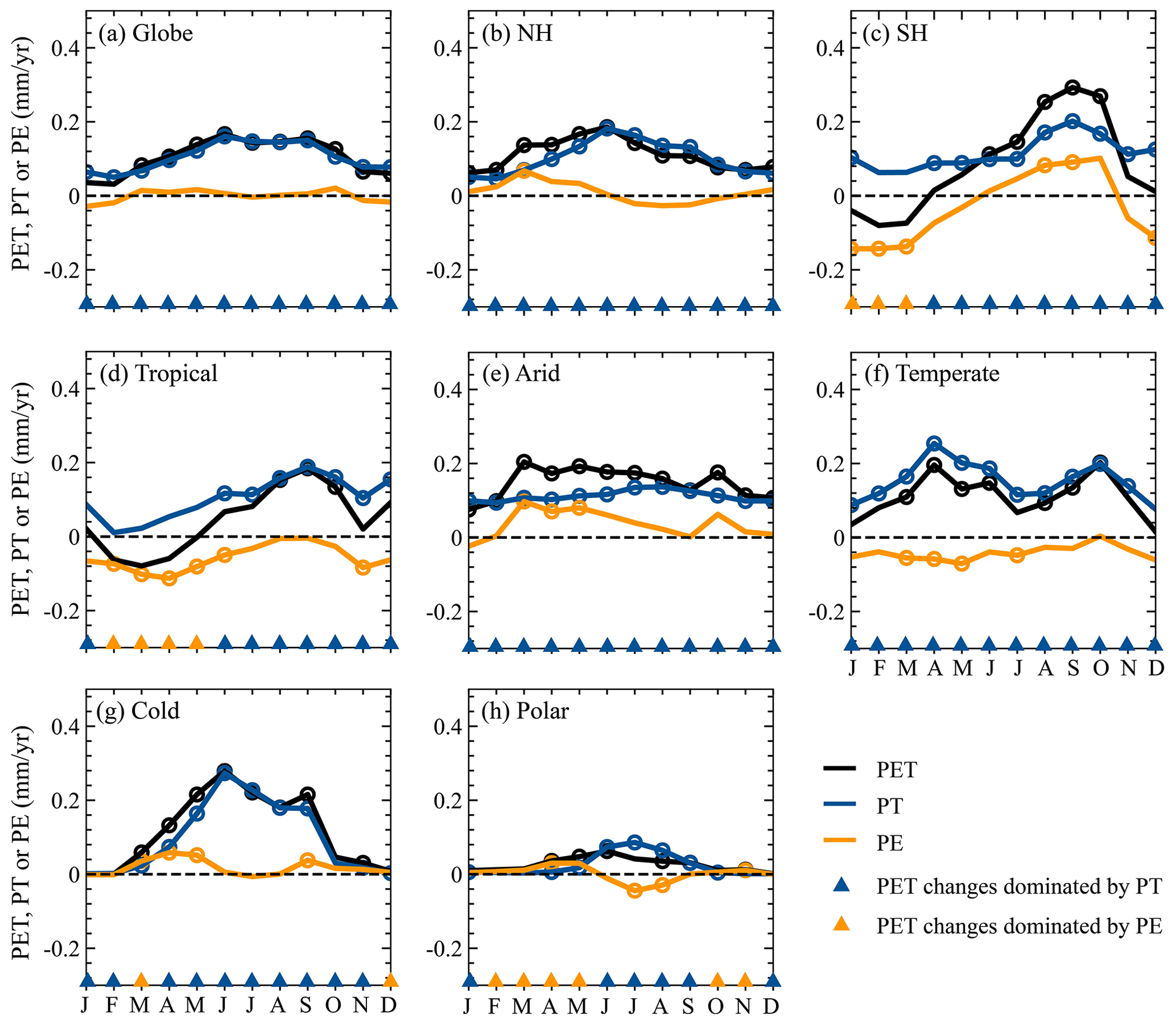
Figure 12 Changes in monthly PET, PT, and PE for the globe, each hemisphere, and each KG climate region. The circle indicates that the trend is significant with p<0.05.

4 Discussion

4.1 Advantages of this new PET dataset and its potential implications

By considering the joint effects of various ET-process-related factors, we have developed a new global PET dataset based on the SW model in this study. This dataset has several advantages relative to existing global PET datasets, e.g., CRU TS4.06 (Harris et al., 2020), MOD16 (Running et al., 2017), GLEAM v3.6 (Miralles et al., 2011; Marten et al., 2017), the PT-JPL model (Fisher et al., 2011), and hPET (Singer et al., 2021). First, the dataset considered more realistic land surface information, including spatial differences in the LULC and vegetation parameters (e.g., canopy height and r_smin) and time-varying LULC and LAI datasets, making the new PET estimates more realistic. Second, the established SW model used in this study was based on more realistic physical processes and gave the SW PET dataset an explicit physical significance, meanwhile providing the PT and PE (which are crucial for understanding PET and ET). Third, a number of studies have found that the elevated atmospheric CO₂ concentration could exert clear impacts on the ET process by controlling plant stomatal resistance (Gedney et al., 2006; Piao et al., 2007; Sun et al., 2014; Roderick et al., 2015; Milly and Dunne, 2016; Yang et al., 2019; Zhao and Cao, 2022). By introducing a stress function of CO₂ concentration to $r_{\mathrm{s}}^{\mathrm{c}}$, our SW PET dataset is able to reflect the impacts of elevated CO₂ on ET.

In view of these advantages, our global PET dataset can apply to multiple properties, e.g., the analysis of rainfall, agriculture, drought, hydrology, and biodiversity. First, our SW PET can provide realistic and physical datasets to further understand the impacts of spatiotemporal differences in rainfall changes from the perspective of scaling effects of the Clausius–Clapeyron relation between air temperature and moisture-holding capacity (IPCC, 2014; Barbero et al., 2017). For example, by exploring the relationships between evaporative demand (even PT and PE) and rainfall, one can re-untangle the different scaling effects of the Clausius–Clapeyron relation between air temperature and moisture-holding capacity. Second, considering PET partitioning into the two components PT and PE, this dataset will be convenient for the agriculture managers for directly using PT estimates for effective agricultural management practices (e.g., seeding, fertilization, irrigation planning, or scheduling) and finally for sustaining the grain yield (Allen et al., 1998; Tomas-Burguera et al., 2019). Third, our SW PET dataset provides an opportunity to further understand drought mechanisms, e.g., how and what magnitudes different PET components (i.e., PT and PE), LULC changes, vegetation greening and elevated CO2-induced vegetation physiological effects (e.g., increased stomatal resistance) impact droughts, which are still unclear at present (Vicente-Serrano et al., 2020). One can use this dataset as input to compute drought indices, i.e., the Standardized Precipitation-Evapotranspiration Index (SPEI) and the self-calibrating Palmer Drought Severity Index (scPDSI) (Wells et al., 2004; Vicente-Serrano et al., 2010), and to separate the impacts of the aforementioned factors on drought evolution. Fourth, the PET as a crucial input for many hydrological models is closely related to the performance of these models (Lu et al., 2003, 2005; Rao et al., 2011; Aouissi et al., 2016; Seiller and Anctil, 2016; Dallaire et al., 2021), and therefore more realistic physical PET estimates will benefit from accurate hydrological modeling and physically understanding hydrological responses to environment changes (e.g., changes in climate and LULC). Fifth, the new PET dataset is of significance for understanding biodiversity responses to local environment changes such as LULC, and PET is usually an effective measure of how climatic energy limits organisms directly and/or influences primary productivity and thus food availability (Kerr, 2001; Hawkins et al., 2003; L. B. Phillips et al., 2010).

4.2 Uncertainties

The estimated SW PET may involve uncertainties from various sources, such as parameterizations of the SW model and inputs for calibrating and driving the model. These uncertainties are discussed in the following sections.

4.2.1 Uncertainties in parameterizations of the SW model

A relatively simple Jarvis-type empirical formula was employed here to describe the impacts of environmental conditions (i.e., temperature, vapor pressure deficit, solar radiation, soil moisture content, and CO₂ concentration) on $r_{\mathrm{a}}^{\mathrm{c}}$. While the better performance is with the Jarvis-type formula in simulating the impacts of environmental conditions on water and carbon fluxes (Jarvis, 1976; Lhomme, 2001; Wang et al., 2020), the interactive effects between environmental factors on $r_{\mathrm{a}}^{\mathrm{c}}$ are not taken into account by this empirical formula. In reality, environmental factors are interdependent, and hence their interaction in the Jarvis-type empirical formula cannot be easily separated. In one word, the “multiplication” form of the Jarvis-type empirical formula potentially biases the estimated $r_{\mathrm{a}}^{\mathrm{c}}$ (Damour et al., 2010; Chen et al., 2022) and then the SW PET estimates.

As an important and undetermined parameter within the Jarvis-type empirical formula for estimating $r_{\mathrm{a}}^{\mathrm{c}}$, r_smin was optimized for FR, SHRB, GRA, and CRO, and the calibrated SW model performance was satisfactory (details in Sect. 3.1). However, it should be noted that this optimized parameter may be the main hindrance to SW model application over the globe (Liu et al., 2003; Mo et al., 2004; Chen et al., 2022). First, r_smin was estimated using EC observations that generally cover the period after 2000 assuming stationary environmental conditions. Environmental conditions were shown to have greatly changed during the past several decades, especially climate conditions such as global warming (IPCC, 2014), brightening or dimming (Wild, 2009), and frequent extreme events (e.g., droughts; Sheffield et al., 2012; Trenberth et al., 2012). Therefore, r_smin may have interannual variations due to the changes in these variables (Wever et al., 2002; Winkel et al., 2001), and this finally introduces biases into the PET product, particularly for years with evidently different environmental conditions relative to the period after 2000 (Aschonitis et al., 2017). Second, r_smin was fixed throughout the year in the SW model, regardless of seasonal variations of this parameter with environmental and vegetation conditions (Winkel et al., 2001; Wever et al., 2002; Douglas et al., 2009). Therefore, no consideration of the seasonal cycle of r_smin may impact the quality of the PET product (Hu et al., 2009; Zhu et al., 2013; Elfarkh et al., 2021). For instance, Hu et al. (2009) and Zhu et al. (2013) found that ET was systematically overestimated or underestimated using the SW model with fixed parameters.

The canopy light extinction coefficient of k_ex, which represents a partitioning of radiant energy over the vegetation canopy and the soil surface, is a key factor affecting ecosystem carbon, water, and energy processes (Tahiri et al., 2006; Zhang et al., 2014). As a result, the accuracy of the SW model was believed to be associated with the k_ex parameterization used in this study. Considering the physiological and morphological differences between terrestrial ecosystems (Emami-Bistghani et al., 2012; Zhang et al., 2014), we followed the popular biogeochemical models and the remote-sensing models of ET and gross primary productivity (e.g., the Lund-Potsdam-Jena Dynamic Global Vegetation Model or the Vegetation Photosynthesis Model; Xiao et al., 2004; Sitch et al., 2003) and assumed this coefficient to be a constant for every LULC type (Table S1). Despite this, it is notable that the k_ex values vary with the growth of plant and/or vegetation coverages (Lindroth and Perttu, 1981; Aubin et al., 2000; Maddoni et al., 2001; Emami-Bistghani et al., 2012; Fauset et al., 2017). Emami-Bistghani et al. (2012) stated that, with an increase in vegetation coverages, the k_ex values decreased, especially at the early reproductive stage in sunflower cultivars. This suggested that the fixed k_ex within the SW model potentially led to uncertainties in the PET estimates. As shown by Tahiri et al. (2006), relative to the values of the variable k_ex, the fixed values gave a less precise estimation of plant transpiration under irrigated maize.

Notably, the SW model only focuses on two processes of ET, i.e., soil evaporation and vegetation transpiration (Shuttleworth and Wallace, 1985). Other parts of ET, vegetation canopy interception and nighttime ET (ET_n), are ignored in this study. It is reported that vegetation canopy interception can occupy a certain proportion in the total ET, especially for regions with a high LAI and frequent rainfall (Gash et al., 1995; Tourula and Heikinheimo, 1998; Lawrence et al., 2007; Wang and Dickinson, 2012). On rainy days, the vegetation canopy interception may account for a considerable fraction of the total ET (Tourula and Heikinheimo, 1998; Hu et al., 2009). On average, the fraction of ET_n accounts for approximately 6.3 % of the total ET informed by the FLUXNET2015 dataset, while 7.9 % is based on multiple global models (Padrón et al., 2020). This fraction may exceed 15 % in a mountain forest with a snowy and windy winter. Despite this, accurately representing the ET_n process is still difficult at present, mainly because the related controlling mechanisms are still not clear (Han et al., 2021). For example, Novick et al. (2009) and Groh et al. (2019) found that vapor pressure deficit (VPD) and wind speed had a significant impact on ET_n, while Groh et al. (2019) stated that the contributions of night dew could not be ignored. As an important component of ET_n, the nighttime transpiration is related not only to the incomplete stomatal closure (Dawson et al., 2007; Duursma et al., 2019), but also to the circular regulation of nighttime water uses by plants (De Dios et al., 2015). However, how the environmental factors alter nighttime transpiration is still disputed. Dawson et al. (2007) and Moore et al. (2008) reported a positive correlation between nighttime transpiration, VPD, and soil moisture content, while Barbour and Buckley (2007), N. G. Phillips et al. (2010), and De Dios et al. (2015) found no or a negative correlation between nighttime transpiration and the two aforementioned variables. Moreover, the biological factors (e.g., plant species and ecosystem types) can also significantly influence nighttime transpiration (O'Keefe and Nippert, 2018; Zeppel et al., 2014). Therefore, establishing a common model for estimating ET_n across various ecosystems remains challenging. All in all, ignoring vegetation canopy interception and ET_n may underestimate PET (Tourula and Heikinheimo, 1998; Lawrence et al., 2007; Mu et al., 2011; Padrón et al., 2020; Singer et al., 2021). Subsequent research will be done to integrate these two processes into the SW model to further enhance the model's physical mechanism.

4.2.2 Uncertainties in datasets for calibrating and driving the SW model

The uncertainties in the EC observations for calibrating the SW model and in inputs for producing the global PET can be propagated into the PET estimates. As for the EC observations, the uncertainties mainly come from the selection of unstressed days for obtaining the observed PET, the issue of non-closure of the energy balance at the EC system level, and the gap-filling methods (e.g., the marginal distribution sampling (MSD) method; Reichstein et al., 2005). The energy-balance-based criterion employed in this study proved to be efficient at selecting unstressed days (Maes et al., 2019), but this method may still result in two uncertainties. First, we should note that the higher the LAI or normalized difference vegetation index (NDVI) is, the larger the EF will be (Gentine et al., 2007; Nutini et al., 2014). This suggests that the larger EF will likely frequently happen during the growing season, which usually corresponds to a higher LAI or NDVI. Therefore, the identified unstressed days tended to involve fewer ones within the non-growing season, potentially introducing large biases into the estimated PET during this season. Second, due to frequent water deficits in arid regions, the EF threshold may exceed the 95th percentile. What is more, there may be no unstressed days in extremely arid regions, mainly because the soil moisture can hardly reach the field capacity or saturation due to the very limited precipitation. Thus, the identified unstressed days using the energy-balance-based criterion may actually include stressed days in arid regions and potentially bias the PET estimates. In order to reduce the impacts of the non-closure of the energy balance in the EC system (Wilson et al., 2002; Foken, 2008), we used the corrected half-hourly or hourly EC LE and H observations and only retained daytime records with a Bowen ratio between 0.90 and 1.10 to calibrate the SW model. Although such processing could reduce uncertainties, the energy imbalance was not fully solved in our study and may lead to inevitable errors in the calibrated parameter of r_smin and therefore the global PET estimates (Hu et al., 2009; Elfarkh et al., 2021; Chen et al., 2022). In this study, to maximize the use of data, the MSD method was employed to fill the gaps in the EC LE measurements. However, we should note that if the controlling thermodynamic and kinetic factors of the atmosphere and soil moisture conditions are different between the missing and retrieved moments, the gap-filled LE based on the MSD method may have low confidence, especially when soil moisture has abrupt changes (Jiang et al., 2022). Recently, Jiang et al. (2022) developed a physics-based full-factorial scheme to fill gaps in ET from EC observations, and they found that the gap-filled ET with this scheme showed higher confidence relative to the existing typical gap-filling methods. Therefore, to reduce the uncertainties from the MSD-based gap-filled LE, the physics-based full-factorial scheme could be a good candidate in the future to fill the ET gaps. Here, to quantify potential impacts of the MSD-based gap-filled values, the SW model was re-calibrated and re-validated against the data points without gap-filling. Relative to the SW model used in this study, the new r_smin and the validation metrics changed insignificantly (Figs. S6 and S7), suggesting that the uncertainties induced by the gap-filled LE were limited.

The SW model used various datasets as inputs, including LULC, LAI, canopy height, and meteorological data (e.g., MSWX-Past, CRU TS4.06, ERA5, and MERRA-2), albeit with some uncertainties (Fang et al., 2013; Xiao et al., 2017; Liu et al., 2018; Xu et al., 2018). As a reflection of vegetation growth, the accuracy of the LAI can affect several key parameters (e.g., $r_{\mathrm{a}}^{\mathrm{c}}$, $r_{\mathrm{s}}^{\mathrm{c}}$, $r_{\mathrm{a}}^{\mathrm{a}}$, or $r_{\mathrm{a}}^{\mathrm{s}}$) and input variables (e.g., A or A_soil) and influence the quality of the PET estimates. To reduce uncertainties from LAI datasets, this study selected the GLASS AVHRR LAI product with a better overall performance (relative to other popular products, e.g., MODIS, FSGOM, GLOBMAP, and GIMMS3g; Fang et al., 2013; Xiao et al., 2017; Liu et al., 2018; Xu et al., 2018). However, we should note that this LAI product slightly underperformed over grassland compared to the other products (Liu et al., 2018). Considering that this LAI product was based on the 8 d maximum value composite for removing the impacts of cloudy days, the LAIe (based on Eq. 3b) was potentially larger than its authentic value due to some leaves being covered by rain or snow. Thus, from Eq. (3b), $r_{\mathrm{s}}^{\mathrm{c}}$ may be slightly underestimated, leading to an overestimation of PT and PET. Considering the impacts of LULC changes on PET across the globe, we used the 1982–2015 yearly GLASS-GLC dataset developed by Liu et al. (2020a, b) to separately estimate the PET for each LULC type. Although the average overall accuracy for the 34 years with seven classes each is 83 % based on 2431 test sample units, the misclassification issues still existed, e.g., in Africa, eastern and southern South America, southern Alaska, northern and eastern Australia, and southwestern Indonesia (Liu et al., 2020a, b). The reconstructed global vegetation canopy height also has limitations, which may arise from (1) uncertainties in the retrieval algorithms and remote-sensing data (Simard et al., 2011; Wang et al., 2016; Potapov et al., 2020; Lang et al., 2021, 2022), (2) neglecting the spatial differences in CRO and GRA heights and using an alternative specific value, and (3) not considering the interannual changes in the FR and SHRB canopy heights and the intra-annual cycle in the CRO and GRA heights. These limitations undermine the accuracy of the PET estimates. Recently, Peng et al. (2022) proposed a practical method for global estimates of 500 m daily aerodynamic roughness length with a combination of machine-learning techniques, a wind profile equation, observations from 273 sites, and MODIS remote-sensing data. Their results showed that the random forest model could reproduce well the magnitude and temporal variability of the daily aerodynamic roughness length at most of the sites for all of the land cover types. We believe that the aerodynamic roughness length produced by this method has the potential to replace vegetation canopy height as an input to run the SW model and thus reduce the aforementioned vegetation canopy height-related uncertainties and improve the accuracy of the PET estimates. A series of evaluations of various meteorological datasets across the world suggested the discrepancies among these datasets (Urraca et al., 2018; Hinkelman, 2019; Jourdier, 2020; Zhang et al., 2021). Although the ensemble mean used here may reduce uncertainties from the meteorological datasets, there is still the likelihood that the remaining uncertainties will be propagated into the PET estimates. In this study, even though soil does experience water stress, we assumed that the soil water supply for ET was unconstrained in estimating PET. As a result, the two conditions with and without soil water stress corresponded to different meteorological variables when considering land–atmosphere interaction (Crago and Crowley, 2005; Kahler and Brutsaert, 2006; Aminzadeh et al., 2016; Maes et al., 2019). For example, air temperature under the unstressed condition will likely be lower than that under the stressed condition because of the lower sensible heating and the stronger evaporative cooling from the wetter land surface to the atmosphere (Maes and Steppe, 2012; Maes et al., 2019). Thus, the mismatch between the assumption of no soil water stress and the observed meteorological variables will likely introduce biases into our PET estimates.

5 Data availability

The product named SW PET with monthly and 5 km resolutions from 1982 to 2015 is freely available at the National Tibetan Plateau Data Center (https://doi.org/10.11888/Terre.tpdc.300193, Sun et al., 2023).

6 Conclusions

This study developed a global 5 km monthly PET dataset during 1982–2015 using the calibrated SW model. The model has been well-calibrated against observations at 96 EC flux sites across four major LULC types: forest, shrubland, cropland, and grassland. We mapped spatiotemporal changes in PET and its components (i.e., PT and PE) across the globe.

Our PET product has three major improvements relative to the existing PET datasets: (1) it provides the PET estimates through clearer physical processes, since we take the spatial differences and temporal changes in land surface properties into consideration; (2) it provides not only PET estimates, but also PT and PE; and moreover (3) it can take the impacts of elevated CO₂ into PET estimation by introducing the stress function of CO₂ to $r_{\mathrm{s}}^{\mathrm{c}}$. This dataset can be used by various scientific disciplines (e.g., agronomy, ecology, climatology, hydrology) and policy-makers for different operational applications.