SCShores: a comprehensive shoreline dataset of Spanish sandy beaches from a citizen-science monitoring programme

Sandy beaches are ever-changing environments, as they experience constant reshaping due to the external forces of tides, waves, and winds. The shoreline position, which marks the boundary between water and sand, holds great significance in the fields of coastal geomorphology, coastal engineering, and coastal management. It is crucial to understand how beaches evolve over time, but high-resolution shoreline datasets are scarce, and establishing monitoring systems can be costly. To address this, we present a new dataset of the shorelines of five Spanish sandy beaches located in contrasting environments that is derived from the CoastSnap citizen-science shoreline monitoring programme. The use of citizen science within environmental projects is increasing, as it allows both community awareness and the collection of large amounts of data that are otherwise difficult to obtain. This dataset includes a total of 1721 individual shorelines composed of 3 m spaced points alongshore, accompanied by additional attributes, such as elevation value and acquisition date, allowing for easy comparisons. Our dataset offers a unique perspective on how citizen science can provide reliable datasets that are useful for management and geomorphological studies. The shoreline dataset, along with relevant metadata, is available at https://doi.org/10.5281/zenodo.8056415 (González-Villanueva et al., 2023b).

1 Introduction

Low-lying coastal zones are the most intensively used regions on Earth for supporting human populations, activity, and industry (Small and Nicholls, 2003). In the European Union (EU) area, 19 % of the population lives within 10 km of the coastal fringe (EEA, 2006). Human pressure contributes to the detriment of coastal environmental systems, making it challenging for coastal managers to find a sustainable balance between the fundamental needs of human and natural coastal systems. Moreover, the latter are highly vulnerable to wave- and storm-induced threats. The presence of coastal depositional systems makes those areas more resistant to these hazards by sheltering them from the full impact. The state of these coastal systems is crucial because they provide the first line of defence against flooding of the hinterland (Arkema et al., 2013; Barbier et al., 2011; Vousdoukas et al., 2020). Considering that sea-level rise and changes in storm tracks, intensities, and frequencies are linked to climate change scenarios, the state of coastal systems should be a worldwide concern because the risks in these highly populated areas are likely to intensify (Oppenheimer et al., 2019; Ranasinghe, 2016; Reguero et al., 2019; Theuerkauf et al., 2014).

Currently, coastal monitoring programmes and sustainable coastal management are priority topics for coastal managers in not only Spain (DGC, 2008; MITECO, 2020) but all EU member states (Farcy et al., 2019). These programmes harvest the knowledge of in situ surveys and remote sensing observations to better understand change and evolution at different spatiotemporal scales, aiming to improve land-use management and infrastructure planning. Extended knowledge of coastal processes has led to increased concern about the state of beaches, as highlighted in the EU strategy on adaptation to climate change (EEA, 2020). Certainly, prioritizing research that emphasizes a swifter and more comprehensive response to the inevitable effects of climate change is a key objective of the EU Action. As such, they are clearly expressed in the Atlantic Action Plan Pillar 4, Goal 6 (European Commission, 2020): stronger coastal resilience, sharing the best practices on the application of maritime spatial planning to coastal adaptation, resilience, and applicable environmental assessments. Additionally, the Ocean Decade Plan (2021–2030) (https://www.oceandecade.org/, last access: 15 May 2023), promoted by the United Nations, establishes 10 challenges for collective impact. These challenges include unlocking ocean-based solutions to climate change, increasing community resilience to ocean hazards, expanding the global ocean observing system, and ensuring skills, knowledge, and technology for all. Therefore, establishing low-cost and accessible monitoring programmes for coastal areas is vital to provide the base data needed to understand the resistance and resilience of sandy beaches. Such an understanding is crucial for achieving the objectives of coastal management and sustainable planning.

Extensive research has shown that coastal systems evolve over time as changes occur in sediment supply and vegetation cover, and their variation mainly depends on primary drivers, namely waves and winds, which in turn show interannual to multi-decadal variability (Castelle et al., 2022; Davis and FitzGerald, 2004; González-Villanueva et al., 2017, 2023a; Masselink and Huges, 2003; Short, 1999). Although there is extensive knowledge about the processes and factors that govern these systems, gaining a thorough understanding of the state of sandy beaches necessitates on-site measurements of their characteristics and information regarding their resistance, recovery, and resilience (Anon, 2022; Kombiadou et al., 2019; Pimm et al., 2019; Masselink and Lazarus, 2019). However, traditional coastal monitoring methods are costly and time-consuming. As a result, the use of combined high-resolution (local) and moderate-resolution (regional) photogrammetry and remote sensing data for coastal monitoring is gaining traction due to its inherent advantages, and more robust methodologies and accessible tools are being developed for both coastal video imaging systems (Andriolo et al., 2016, 2019; Montes et al., 2018, 2023; Sánchez-García et al., 2017) and satellite imagery (Andriolo et al., 2016; Sánchez-García et al., 2019, 2020; Vos et al., 2019). Nevertheless, the potential of these methods for coastal monitoring has not yet been fully exploited, and their effective utilization requires professionals with high levels of expertise.

In addition, citizen science projects have been growing in number and importance over the past decade. These types of initiatives not only yield a large amount of data that would otherwise be very expensive or impossible to obtain, but they also serve to raise awareness among the general public about some problem, usually of an environmental nature. There are four common features of citizen science projects: (1) anyone can participate, (2) participants use the same protocol, so data can be combined and be of high quality, (3) data can help real scientists come to real conclusions, and (4) a wide community of scientists and volunteers work together and share data to which the public, as well as scientists, have access (Flagg, 2016).

Given the current challenges posed by the limited availability of in situ observation data for understanding shoreline response, and due to significant advancements in smartphone camera lens technology together with the increasing use of social media, the CoastSnap international citizen-science initiative emerged in 2017 as a low-cost cutting-edge shoreline mapping approach that leverages crowdsourced images (Harley et al., 2019). In Spain, the CoastSnap network was established in 2018 at Rodas Beach (National Park of the Atlantic Islands of Galicia), and has grown moderately since then. The support of a project funded by the Spanish Foundation for Science and Technology (FECYT) named “Centinelas de la Costa” (FCT-20-15835) has facilitated its expansion since 2021 and the addition of new stations for nationwide dissemination. Currently, there are 22 CoastSnap stations (CSs) along the Spanish Atlantic and Mediterranean coasts, completing the network (Fig. 1), which is expected to expand in the forthcoming years. This paper introduces SCShores, a citizen-science dataset of geographically corrected shorelines obtained for five stations in the Spanish CoastSnap network. SCShores includes shoreline positions from sandy beaches with meso- to micro-tidal regimes representative of the northwest, southwest, and east coasts of Spain. A total of 1721 individual shorelines composed of points every 3 m along the shore are delivered, accompanied by additional attributes such as tide level, timestamp, and image source, which allow for easy exploitation. The paper offers a comprehensive description of the process involved in building the SCShores dataset, along with its limitations and potential applications for different end-users. SCShores v.1.0 is designed to be analysed easily using data science tools and geographic information system (GIS) software.

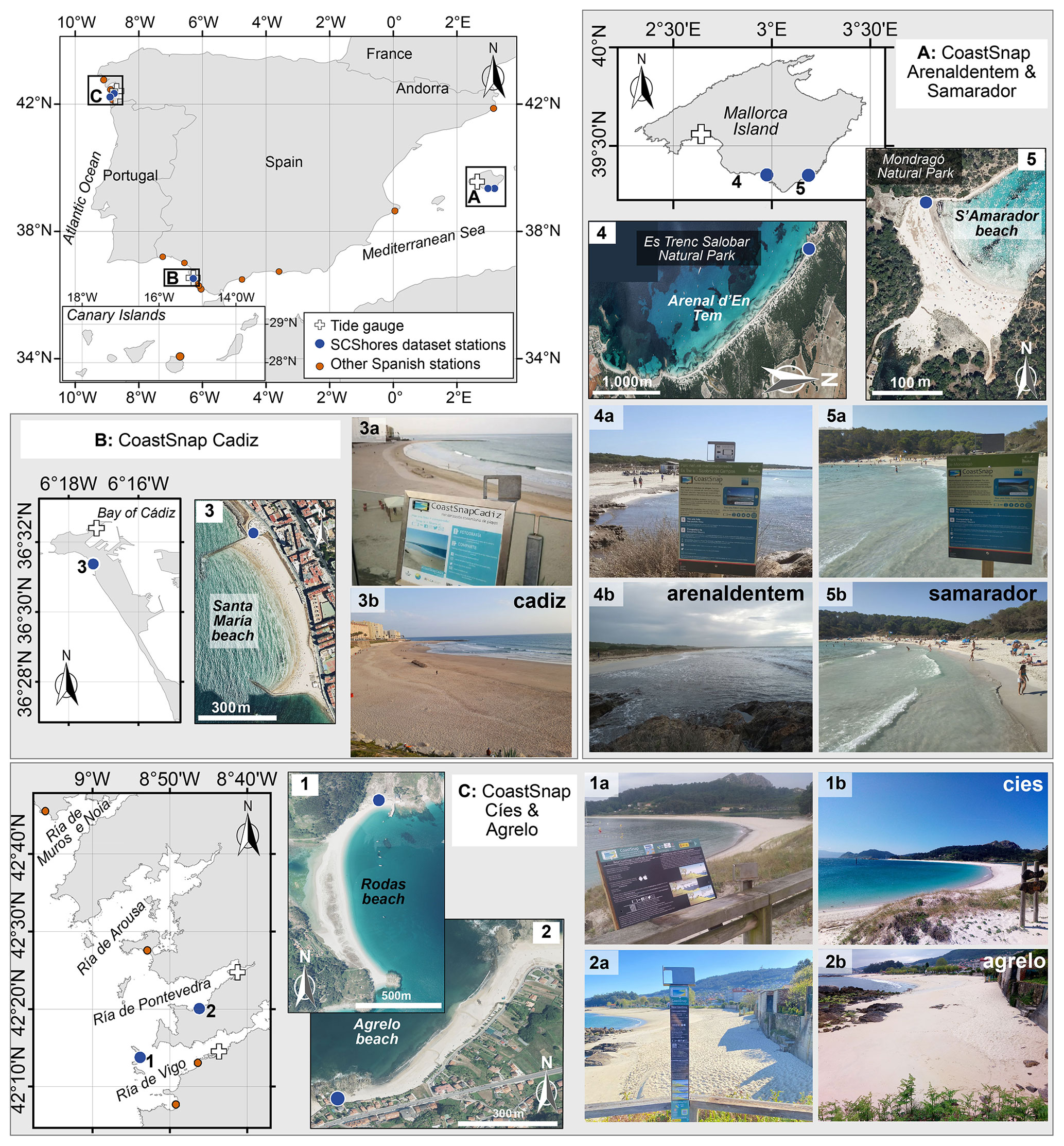
Figure 1 The Spanish CoastSnap Network, including all existing stations in May 2023 (represented by blue and orange dots), along with the tide gauges (depicted as crosses) used in the SCShores v1.0 dataset, which corresponds to the five stations in the SCShores dataset. Photographs of the SCShores CoastSnap stations (1 to 5a) and beach views from each station (1 to 5b) are also shown. The backgrounds used for the location maps are orthophotos from PNOA (national plan for aerial orthophotography in Spain) sources (CC-BY 4.0, https://scne.es 2021 (last access: 20 May 2023)) and the European boundary layer downloaded from http://www.efrainmaps.es (last access: 20 May 2023) (Carlos Efraín Porto Tapiquén – Geografía, SIG y Cartografía Digital, Valencia, Spain, 2020).

2 Methods

2.1 Study sites and CoastSnap station settings

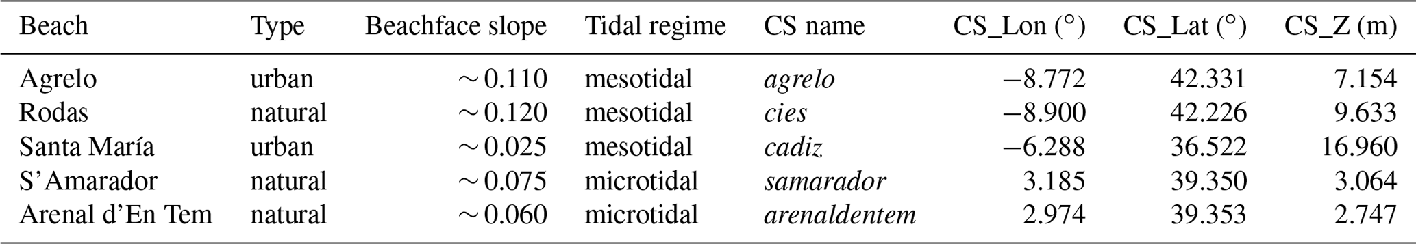
The SCShores v.1.0 dataset comprises five Spanish CoastSnap stations that were specifically chosen for this project. Three of these CSs are located on mesotidal beaches, while the remaining two are on microtidal beaches (Fig. 1 and Table 1). These five stations were selected as they had larger amounts of available images and validation data than the others, with consideration given to both meso- and micro-tidal beaches. Plates with a thickness of 6 mm were selected for the grade 316 stainless steel used in crafting the CoastSnap cradles. These bases were securely affixed to existing infrastructures or dedicated wooden posts bolted to rocky substrates, ensuring their stability and preventing any movement. A brief description of each coastline sector and its corresponding station is provided below.

Table 1 Beach characteristics and CoastSnap stations (CSs) used for the SCShore dataset. The positions of the CSs are given in World Geodetic System 1984 coordinates (CS_Lon, CS_Lat), and the elevations (CS_Z) are referenced to the mean sea level in Alicante (NMMA; Spanish vertical datum).

Mesotidal beaches:

• 1.

  Rodas beach. Situated on the sheltered eastern margin of the Islas Cíes archipelago at the mouth of the Ría de Vigo on the northwest coast of Iberia, this beach forms part of a sand barrier characterized by a well-developed foredune that surrounds a shallow saline lagoon. The sandy barrier serves as a natural connection between the two northern islands within the archipelago and is recognized as a significant ecological feature within the National Park of the Atlantic Islands of Galicia. 1.2 km in length, this beach is classified as a low-energy beach with a reflective morphology (Costas et al., 2005) and a spring tidal range that can reach up to 4 m. Tourist activity is primarily concentrated during the summer season. The CoastSnap station (cies), installed in April 2018, is positioned on an elevated wooden pathway across the dunes in the northern region, providing a southward view of the beach (Fig. 1). Using GPS RTK-GNSS, a total of 10 ground control points (GCPs) and 14 in situ water lines were measured for rectifying the obtained images and validating the mapped shorelines, respectively.

• 2.

  Agrelo beach. Located on the northwest coast of Spain in the inner part of Ria de Pontevedra (Fig. 1), this coast is under a meso-tidal regime, with a spring tidal range of 4.5 m. It is classified as a reflective beach and often presents beach cusps and beach steps. The beach is situated in a densely populated area that experiences a significant influx of tourists during the summer season. It is also backed by human-made infrastructure, including houses and a walkway. The CoastSnap station (agrelo), installed in January 2019, is positioned on a viewpoint at the southern entrance of the beach, providing a northeast beach view (Fig. 1). Using GPS RTK-GNSS (real time kinematics global navigation satellite system), a total of 16 GCPs and 11 in situ water lines were measured.

• 3.

  Santa María beach. Located on the southwest coast of Spain, Santa Maria del Mar is an urban pocket beach, NNW-SSE oriented, which is located in the city of Cádiz (Fig. 1). It has a length of 600 m and is strongly controlled by morphological contour conditions. It is backed by a high cliff protected by a revetment with a sea wall at its toe. The beach is limited at its northern and southern ends by two jetties normal to the shoreline. It is classified as an intermediate-dissipative beach with a common presence on intertidal sandbars. This is a low-energy coast with a mean spring tidal range of around 3 m. The CoastSnap station (cadiz), installed in October 2020, is positioned on a viewpoint at the northern entrance of the beach, providing a southeast beach view (Fig. 1). Using GPS RTK-GNSS, a total of seven GCPs and three in situ water lines were measured.

Microtidal beaches:

The S'Amarador and Arenal d'En Tem beaches on Mallorca Island (NW Mediterranean), are characterized by microtidal conditions with a tidal range of ∼ 0.2 m. However, sea levels vary from 0.5 to 1 m due to multiple factors such as atmospheric and wind-induced surges, inter-annual variations in sea temperature, internal oscillations in the Mediterranean basin, and the interaction of internal currents in the Western Mediterranean (Haddad et al., 2013; Orfila et al., 2005). During the tourist season (June to September), both beaches experience high levels of occupancy.

• 4.

  S'Amarador beach. Located on the Mondragó Natural Park (Fig. 1), S'Amarador is an enclosed sandy beach associated with a gully and constitutes the barrier of a small lagoon. The CoastSnap station (samarador) was installed in July 2022; it is positioned on a walkway at the north of the beach, providing a longitudinal southeast view of the shoreline (Fig. 1). Using GPS RTK-GNSS, four GCPs and five in-situ water lines were measured.

• 5.

  Arenal d'En Tem beach. Located in the Es Trenc-Salobrar Natural Park, Arenal d'En Tem is part of one of the most emblematic coastal stretches of Mallorca Island (Fig. 1). From a morphodynamic perspective, this beach alternates between intermediate and reflective states in the winter and summer seasons, respectively. The CoastSnap station (arenaldentem) was installed in September 2022; it is positioned on a walkway at the northwest end of the beach (towards the seawater), providing a southeast view (Fig. 1). Using GPS RTK-GNSS, eight GCPs and two in situ water lines were measured.

All GCPs selected for this study correspond to fixed points that are easily identifiable within the target image. These GCPs encompass various types of features, including natural elements such as rocks and outcrops as well as man-made structures like houses and maritime or beach infrastructure.

2.2 Dataset generation

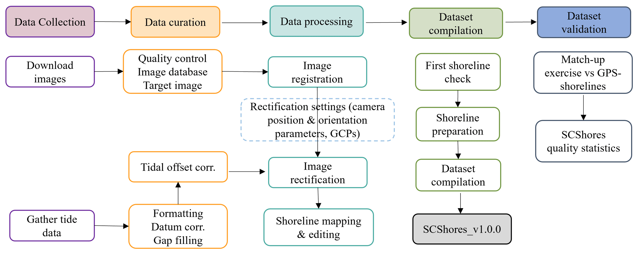
The process of generating the dataset involved five main steps: data collection, data curation, data processing, dataset compilation, and dataset validation. The dataflow diagram outlining the process for creating SCShores_v1.0 is summarized in Fig. 2.

Figure 2 Data flow diagram for the generation of the SCShores dataset.

2.2.1 Data collection

The data collection process adheres to the standards established in the CoastSnap global citizen programme, which monitors changing coastlines (Harley et al., 2019; Harley and Kinsela, 2022). At each CS, users are given specific instructions on how to share their images, including via social media (Instagram, X (formerly Twitter), and Facebook), email, and the web, and a dedicated smartphone application (CoastSnap App). The procedure used for downloading images depended on the sharing medium chosen by the user. As the study beaches have varying tidal regimes, it is necessary to maintain a tidal record to establish the tide level in each photo. This is used in the image rectification step (Fig. 2) and allows the end-users to conduct temporal analyses under the same sea level conditions. The tidal record was gathered from the closest available tide gauges (Table 2). Due to the absence of a local tide gauge at the beach, local tidal offsets were determined for each beach. This was accomplished by comparing the in situ measurements acquired using GPS RTK-GNSS (Z_GNNS) with the corresponding records from the tide gauge (Z_Tide) for the same time period. Tidal height measurements on the beach were obtained simultaneously while measuring the waterline using GPS RTK-GNSS in order to cover various meteorological scenarios, including both high- and low-pressure systems as well as varying wave conditions. The differences (tidal offsets) between tide levels at the beach and the tidal gauge were calculated and averaged by site. The accuracy of the determined local offsets was later confirmed by comparing these shoreline elevation measurements (Z_GNNS) with their corresponding estimated tidal values (Z_Tide + tidal offset) used as the CoastSnap shoreline elevation (Fig. 3) for the same dates. The shorelines obtained from the agrelo, cies, and cadiz CSs, which are mesotidal, may exhibit greater displacement from the reference line due to the temporal variations in tidal levels and the availability of multiple measured shorelines for the same date.

Table 2 Tide-gauge locations and characteristics used in SCShores. The tidal offset for each study site was obtained by calculating the difference between the in situ measurements obtained using GPS RTK-GNSS and the corresponding tide-gauge records for the same time. ΔZ (m) is the difference between each tide gauge zero reference and the NMMA (Spanish vertical datum).

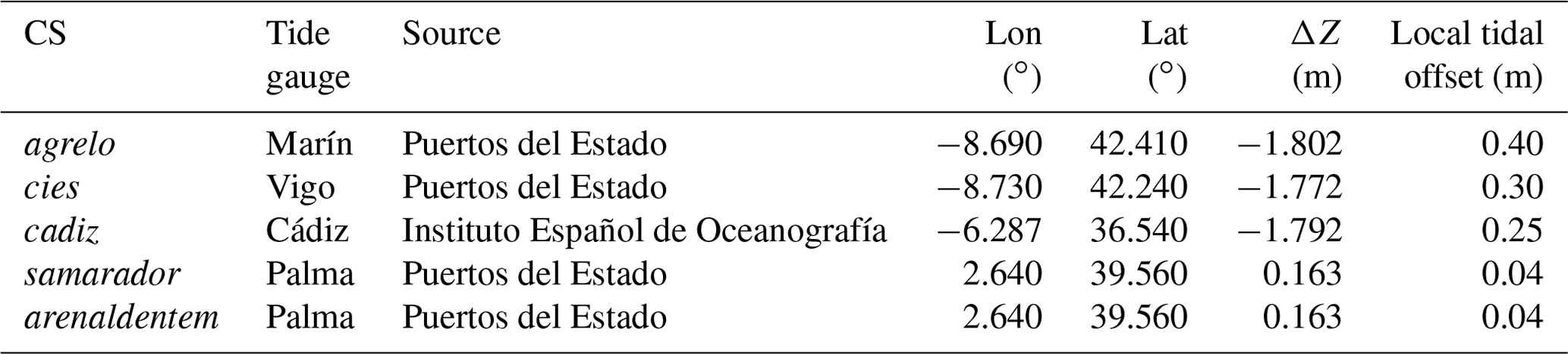
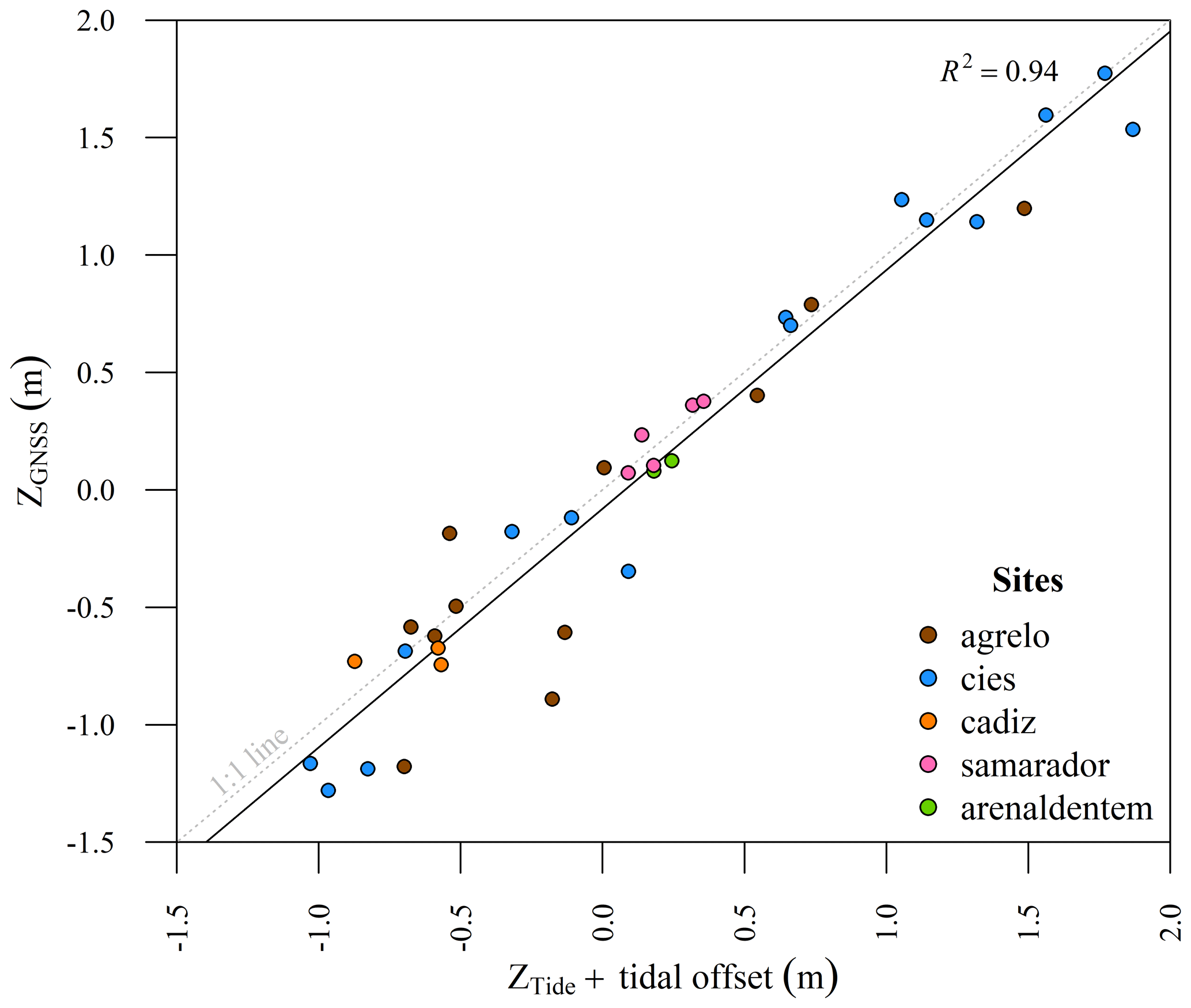
Figure 3 Comparison of estimated tidal elevation used as the CoastSnap shoreline elevation (Z_Tide + tidal offset) with their corresponding measured shoreline elevation values (Z_GNSS) for the same dates (refer to coincident days in Fig. 8).

It is important to note that precisely resolving the complex interplay among various influential factors in shoreline elevation (e.g. bathymetry, significant wave height, wave period, wave direction, winds, run-up) requires the utilization of sophisticated models that rely on in situ data. However, such data is often deficient, as is evident in the study areas under consideration. While this circumstance might introduce a degree of uncertainty, the computation of the vertical tidal offset employed in generating the provided dataset is inherently straightforward. This approach aligns with the corrective methodology proposed within the CoastSnap framework and mitigates errors associated with the aforementioned factors in the estimation of shoreline elevation (Harley et al., 2019).

2.2.2 Data curation

The data provided by CoastSnap users comes from multiple sources and different models of smartphone. Given that most of the image downloading process is automated, it is necessary to perform a manual verification of the received data to eliminate duplicate records, incorrect captures, or irrelevant images. Additionally, quality control of the date and time of the snap must be addressed to ensure the correct tide level assignment in photos for which the original metadata were lost, such as those downloaded from social media (Facebook, Instagram, X). A time stamp quality (TSQ) attribute was set for each image. TSQ = 1 was assigned to images for which the users specified the date and time in comments in social media posts and emails, and to images that preserved original metadata or were uploaded to the CoastSnap App, which requires the user to confirm the capture date and time. TSQ = 2 was assigned to images which are expected to be uploaded and sent at the time of capture but are not accompanied by any comment. Consistency between the defined date and time and the lighting conditions depicted in the images was also visually checked for each image. Images which were considered unreliable or lacked date or time descriptors were rejected.

The data gathered from tide gauges need to undergo quality control before they can be used (Fig. 2). This included: (1) homogenizing the temporal resolution (to 15 min), time zone (transformation to UTC), and vertical datum reference (corrected to the sea level reference, NMMA; Table 2); (2) filling gaps in tidal records using the T_TIDE routine (Pawlowicz et al., 2002) and the linear fitting of tide predictions with the measured tide; and (3) formatting the data series structure to meet the requirements of the CoastSnap-toolbox.

2.2.3 Data processing

The data processing flow comprises three consecutive procedures (Fig. 2): image registration, image rectification, and shoreline mapping and editing.

The image registration process involves aligning all available images per station with a target image. This process was performed using Adobe Photoshop software. The registered images were georectified to transform the image from pixel coordinates (u,v) to world metric coordinates ($X,Y,Z$). To accomplish this transformation, GCPs associated with known pixels of the target image and the position of the station (both measured accurately in the field with a GPS RTK-GNSS) and the station-view orientation parameters (measured with a spirit level) are required. This process was performed by using the CoastSnap toolbox and the procedure described by Harley et al. (2019). The dynamic shoreline indicator extracted from these images corresponds to the instantaneous upper edge of the swash zone, which is highly dependent on the tidal level at the time of photo capture. The toolbox employs the tide elevation value as the Z coordinate or projection value, which is considered the sum of the tidal record and the tidal offset corresponding to the date and time of the captured image. This approach accurately locates features with such a Z value, i.e. the shoreline, in the georectified image.

The CoastSnap toolbox employs an automatic method for shoreline mapping based on applying a dynamic threshold to the blue minus red band combination, which is intended to maximize the difference between dry and flooded surfaces. The performance of this method can be influenced by various factors, including the light conditions, the presence of wet sand, flooded areas, shadows, and the wave conditions. To ensure data consistency, we specifically focused on mapping the dynamic shoreline, thus excluding terraces or flooded onshore beach areas (Fig. 4). As there is not always a straightforward interface between sand and water, all mapped shorelines underwent meticulous examination by an expert and were edited as needed. The shoreline vertices were manually repositioned to adhere to the dynamic water conditions and were interpolated using cubic splines, assuring that the lines intersected all manually adjusted vertices and achieved an average point spacing of 3 m.

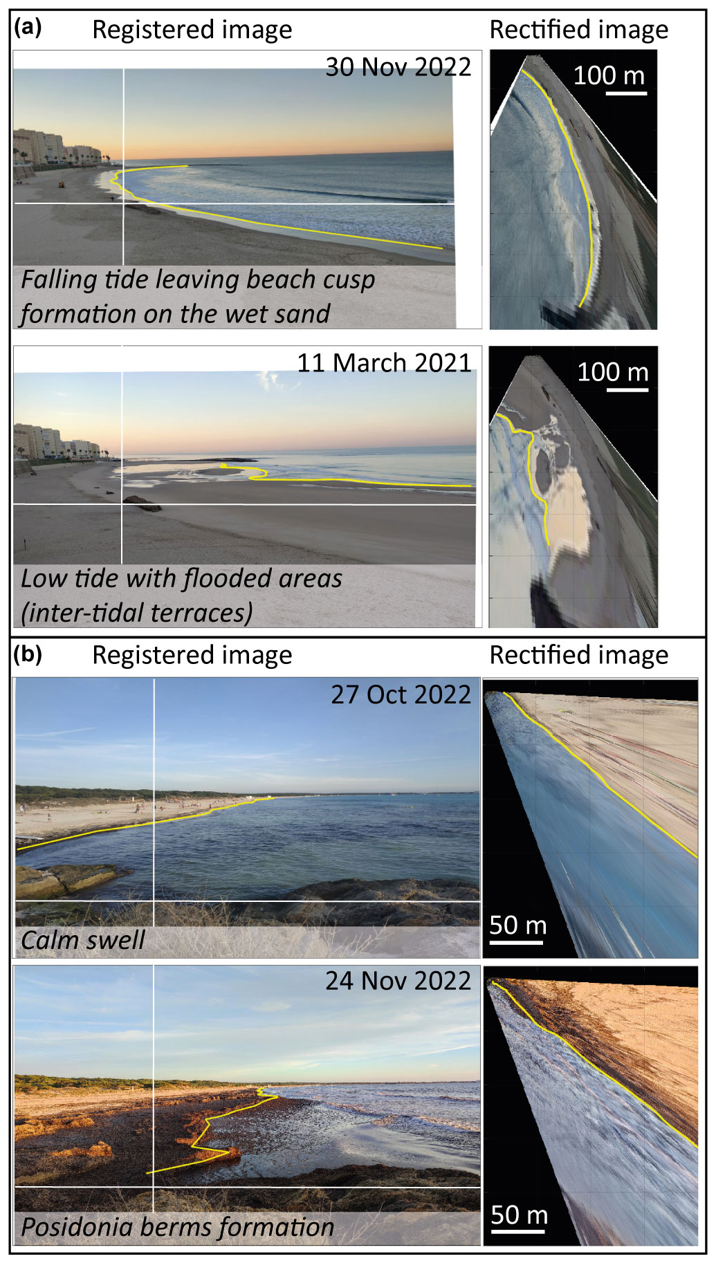
Figure 4 Examples of four different scenarios at (a) the CoastSnap cadiz and (b) the CoastSnap arenaldentem stations, where the “dynamic water” shoreline is mapped (yellow line) in both the registered images (oblique images) and rectified images (plan-view images).

2.2.4 Dataset compilation

Before assembling the edited shorelines into a unified dataset, it was essential to identify and exclude shoreline segments where cumulative errors from image acquisition properties and processing methods could introduce significant inaccuracies. Since data provided by users are captured from different smartphones with different camera focal lengths, the resulting images have different dimensions in terms of width and height (i.e. pixel count). In the best-case scenario, the original dimensions are preserved, such as in the images sent by email with full resolution. However, in most cases, the original pixel size is not retained due to image compression policies enforced by social media platforms and the CoastSnap App. Platforms like Instagram, X, and the CoastSnap App typically limit image dimensions to a maximum width of 1080, 1200, and 1920 pixels, respectively. Following the registration process, all images are standardized to the resolution of a corresponding target image (Table 3). However, larger disparities between the target and registered images require further significant interpolations, resulting in greater deformations and increased uncertainty in the final pixel positions.

Table 3 Factors that limit the spatial resolution of georectified images. These factors include the field of view (FOV) in degrees, the elevation of the station above sea level (CS_Z), and the resulting pixel resolution at distances of 150 and 450 m for both the cross-shore component (Ac) and the long-shore component (Ar).

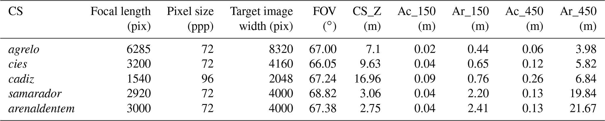
Apart from the image resolution, the view of the capture (perspective) is also an important parameter to consider for understanding the error propagation during the resection (i.e. recreating the geometry of a photographic shot) and rectification processes. Images taken closer to the zenithal plane show lower distortion of the pixels in the image. In this work, this is related to the elevation of the CS at each site and the length of the shoreline (distance to the camera). Broadly, a larger focal length and higher elevation led to higher resolution of the georectified image, resulting in a smaller long-shore pixel footprint. This is illustrated in Table 3 and Fig. 5, where long-shore pixel footprints are calculated according to the Holman and Stanley (2007) formulations for different pixel widths and various camera elevations, including those that apply to the present study cases, demonstrating the relevance of both parameters in reducing the far field pixel size and thus the plausible resolution of the extracted shoreline.

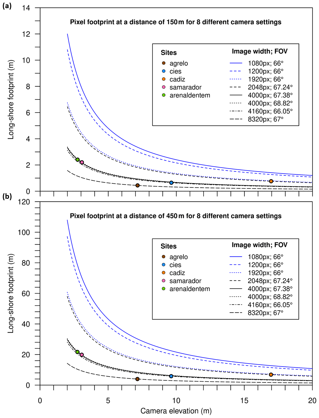
Figure 5 Long-shore footprints at distances of 150 m (a) and 450 m (b) for eight different camera scenarios, taking into account the elevations of the stations. The camera settings correspond to typical social network images (blue) and the characteristics of the different target images used in the present study (black). The use cases corresponding to the values of Ar in Table 3 are also presented (CS sites).

In the best scenario, the resolution of the long-shore pixel exhibits oscillations of approximately 0.44 and 3.98 m at distances of 150 and 450 m, respectively (agrelo, in Table 3). However, this resolution worsens to 2.41 m (at 150 m distance) and 21.67 m (at 450 m distance) in the case of the lowest-elevation CS (arenaldentem; Table 3). Due to the increasing pixel footprint, the accuracy of shoreline mapping is compromised, and manual digitization of the shoreline through visual photointerpretation in the study sites becomes impractical beyond the 450 m threshold. Consequently, data points beyond this distance were trimmed and excluded from the analysis. Furthermore, the presence of site-specific geomorphological features such as a greater slope or a curved planform, along with methodological constraints including the number and image distribution of the GCPs as well as the view of the beach from the station, can contribute to increased errors during rectification and digitization processes. Hence, it is imperative to adjust the shoreline cutoff distance based on the CS characteristics at each site to account for these factors. To enhance the overall precision of the extracted shorelines, a comparison was conducted between the water lines measured using GPS RTK-GNSS and those derived from CS data (the procedure named “first shoreline check” in data flow of Fig. 2). This comparison involved analysing the XY deviation between the two datasets, considering both timestamp and site information. The XYZ distance to the station, as depicted in Fig. 6, was considered during the assessment. Validation solely utilized GPS RTK-GNSS measurements due to their widespread availability and unmatched precision (≤ 15 cm) across all three spatial dimensions ($X,Y,Z$). High-resolution satellite images (< 50 cm² pixel size), although accessible, require funding as they originate from commercial platforms like WorldView2/3. Their spatial accuracy relies on both pixel size and georeferencing precision, introducing potential uncertainties into shoreline position and the further validation of CoastSnap shorelines.

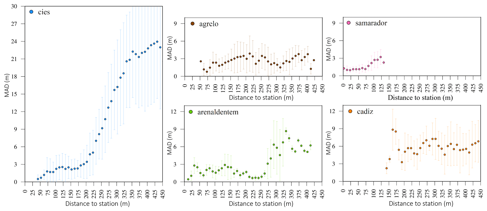
Figure 6 Mean absolute distance (XY) between CoastSnap and GPS RTK-GNSS coincident shorelines at different sections along the distance to station (XYZ) and for each site within a cutting point range of [0, 450] m. Each bar represents the standard deviation.

The comprehensive analyses conducted in this study contributed to the determination of the optimal XYZ distance between shoreline points and the CS for precise and reliable shoreline mapping. In order to ensure the optimal representation of each site, the extracted shorelines were carefully trimmed to the appropriate distances, as summarized and explained in Table 4. The influence of this cutoff distance on the retained shoreline length is shown in Fig. 7.

Table 4 Maximum distance that ensures shoreline mapping accuracy for each CoastSnap station in SCShores. See Fig. 7 for reference.

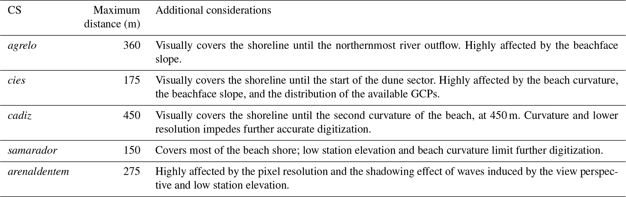
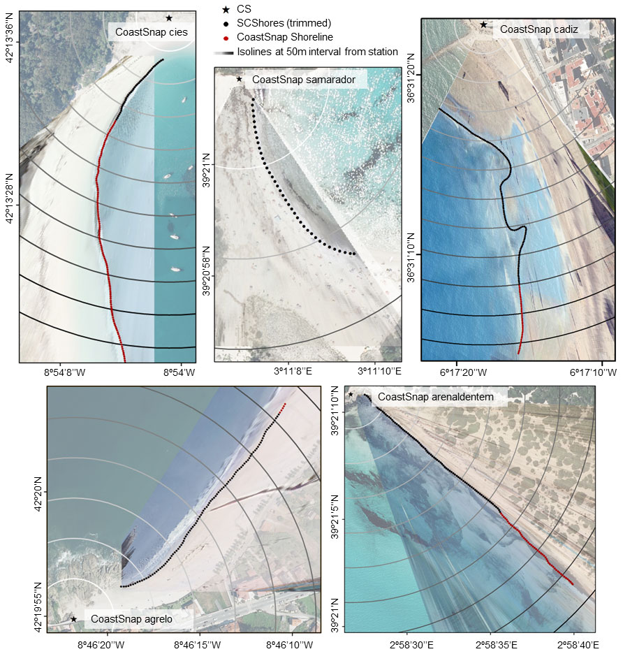
Figure 7 Rectified CoastSnap photographs for each site that showcase the entire mapped shoreline (highlighted in red) and the resulting shorelines after trimming (depicted in black) in accordance with the optimized distances detailed in Table 4. The isolines, delineated at 50 m intervals, denote the plain distances from the CoastSnap stations, thereby providing a spatial reference within the SCShores dataset. The backgrounds used for the rectified photos are orthophotos from PNOA sources (CC-BY 4.0 https://www.scne.es/ 2021 (last access: 20 May 2023)). The grid coordinates are GCS_WGS_1984.

The next step entailed the homogenization of the coordinate reference system. All the shorelines were reprojected to a single coordinate system, WGS84 (EPSG: 4326), as the data covered different UTM zones. Finally, all the shorelines were compiled into a single dataset (SCShores v1.0) using the GeoJSON format (Butler et al., 2016), an open standard for representing geographical features and their associated non-spatial attributes.

2.2.5 Dataset validation

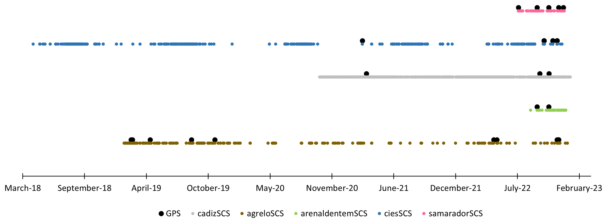
For the final dataset validation, the same in situ GPS RTK-GNSS shoreline measurements at CoastSnap sites used in the previous section were utilized. These measurements adhered to the same criteria employed for mapping shorelines, which involved identifying the dynamic shoreline. The validation process comprised several consecutive steps. Initially, a match-up exercise was conducted to select the CoastSnap-derived shorelines (SCShores_v1.0) that closely corresponded in time with the in situ measured ones acquired on the same date. The identified shoreline matches can be observed in Fig. 8. The average time difference between the measurements was ±11.4 min. The number of match-ups per site was variable, with two GPS-measured shorelines for arenaldentem, five for samarador, 14 for cies, 11 for agrelo, and three for cadiz. To assess the accuracy, the shorelines extracted from CoastSnap were trimmed to align with the corresponding GPS-measured ones. This alignment was achieved by defining a linear area that covered the maximum lengths of the measured lines. The trimmed shorelines were then validated through a point-to-point analysis. For each point along a CoastSnap-derived shoreline, the minimum Euclidean distance to the corresponding measured shoreline point was calculated as in Eq. (1):

$$\begin{array}{}\text{(1)}& {\mathit{\gamma }}_i=M_i-O_i,i=\mathrm{1},\mathrm{\dots },n,\end{array}$$

where M_i are the SCShores-mapped points and O_i are the measured ones, and n is the number of points mapped along the shoreline. Then, the distances γ_i were used to calculate different evaluation metrics both globally and per site. These metrics included the mean absolute distance (MAD, Eq. 2); the root mean square distance (RMSD, Eq. 3), the percentage probability of γ being less than or equal to 3 m (P3, Eq. 4), and the value corresponding to the 75th percentile of the computed distances (Q3).

$$\begin{array}{}\text{(2)}& {\displaystyle }\mathrm{MAD}={\displaystyle \frac{\mathrm{1}}{n}}{\sum }_{i=\mathrm{1}}^n\left|{\mathit{\gamma }}_i\right|,\text{(3)}& {\displaystyle }\mathrm{RMSD}=\sqrt{{\sum }_{i=\mathrm{1}}^n{\displaystyle \frac{{\mathit{\gamma }}_i^{\mathrm{2}}}{n}}},\text{(4)}& {\displaystyle }P\mathrm{3}={\displaystyle \frac{n_{\left[\left|{\mathit{\gamma }}_i\right|\le \mathrm{3}\right]}}{n}}\times \mathrm{100}.\end{array}$$

Figure 8 Timeline of SCShores_v1.0 coastlines and GPS RTK-GNSS measurements.

2.3 Dataset description

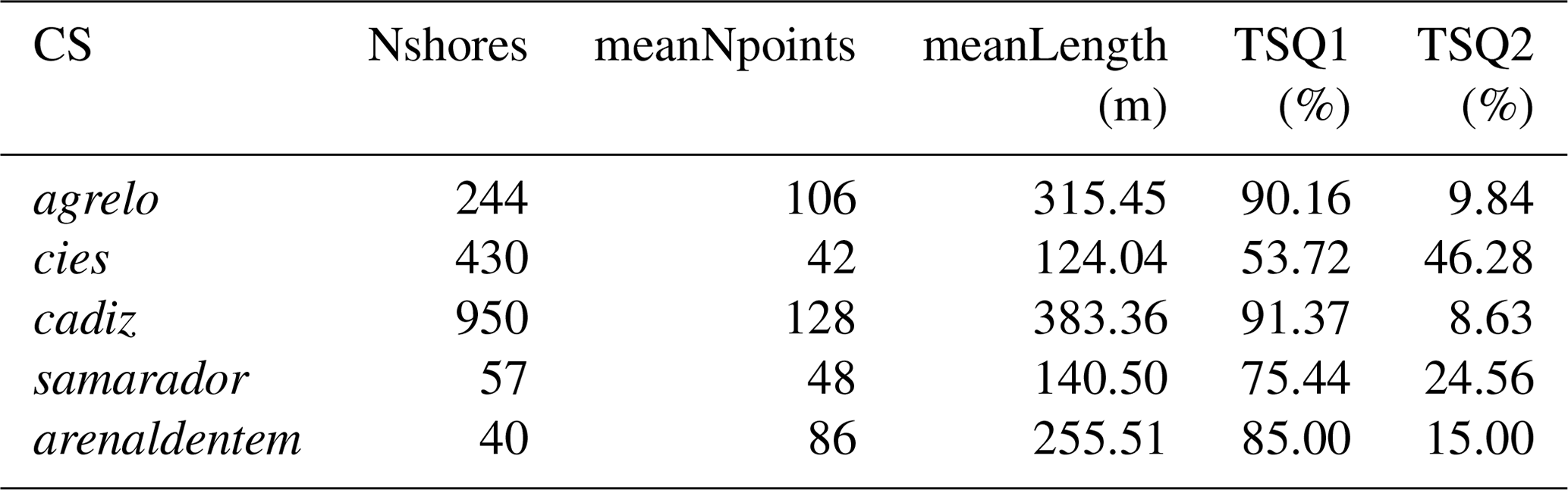
The SCShores v1.0 dataset is available in the form of a single geospatial layer, specifically a GeoJSON file. In total, the dataset comprises 1721 shorelines, which monitor a coastal extension of roughly 1.3 km between April 2018 and December 2022 (Fig. 8). The number of shorelines per site is variable (as outlined in Table 5), ranging from 40 for the site arenaldentem (active since July 2022) to 950 for the site cadiz (active since September 2020). ∼ 80 % of the acquired shorelines correspond to a TSQ rating of 1 (Table 5), signifying high reliability of the obtained shorelines.

Table 5 Summary of SCShores_v1.0 content per study site. CS: name of the CoastSnap station; Nshores: number of shorelines per site in the dataset; meanNpoints: mean number of shoreline points per site; meanLength: mean length of the obtained shorelines per site in the dataset. TSQ1 and TSQ2 correspond to the percentages of shorelines with a timestamp flag equal to 1 and 2, respectively.

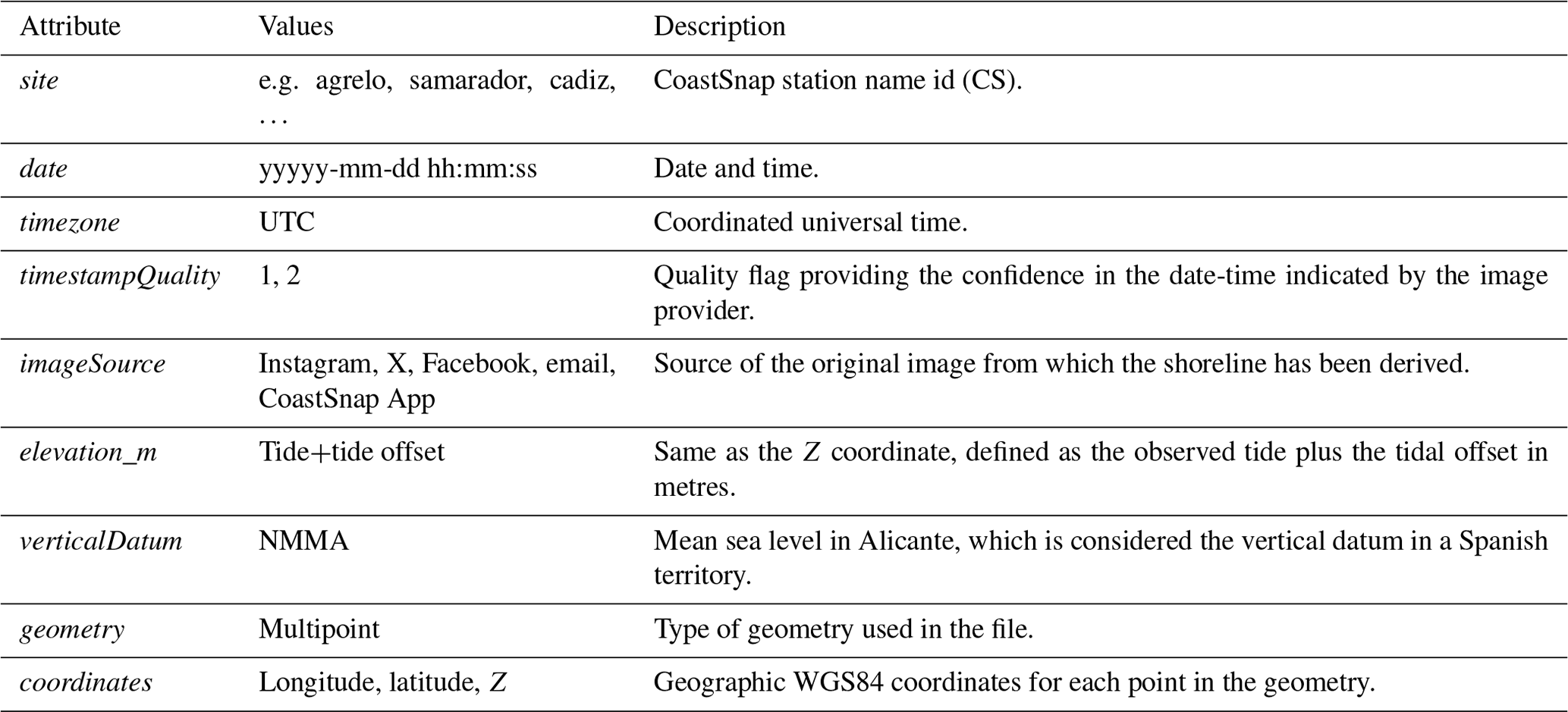
The GeoJSON file consists of a feature collection of multipoint geometries (Lon, Lat, Z) in the WGS84 coordinate reference system (EPSG: 4326) corresponding to the mapped shorelines for each available date and time. Each shoreline in the collection is associated with seven additional attributes (Table 6).

Table 6 Description of data fields for the SCShores_v1.0 dataset at the individual shoreline scale.

3 Results and discussion

3.1 SCShores v1.0 performance assessment

Overall, the methodology used enabled the extraction of shorelines with an approximately 67 % probability of the error being less than or equal to 3 m, and a 75 % probability of it being less than 3.8 m (Table 7). For each site, the mean absolute distance (MAD) relative to the distance from each station and taking into account the varying shoreline elevation is shown in Fig. 6.

Table 7 Descriptive statistics for individual sites and combined data. N_GPSshores corresponds to the number of available in situ GPS measured shorelines per site, and N_points indicates the number of SCShores points that were compared to compute the statistics (see Sect. 2.2.5).

This study identifies several factors that contribute to the potential errors in shoreline extraction when using the CoastSnap methodology. These factors include registration and image resolution; the spatial resection process and rectification (involving the number and suitability of GCPs); tide bias; beach shape and morphology (e.g. planform curvature, beachface slope, or the presence of sand bars and troughs); and the position of the CS (Table 4), including the distance and orientation to the shoreline position.

The highest accuracies were achieved for microtidal sites, while the poorest results were obtained for the cadiz site. However, it is important to note that this does not necessarily imply that shoreline accuracy is inherently lower in mesotidal areas. The uncertainty associated with the swash zone in areas with a very low slope and the presence of bars such as Santa María beach (cadiz CS) creates greater uncertainty when measuring (in the field) and mapping the water line due to the presence of a water sheet. Therefore, the observed differences in accuracy are attributed to these specific challenges encountered in mesotidal zones rather than a limitation inherent to the CoastSnap methodology.

3.2 Limitations of the dataset

The limitations of the dataset originate from temporal and spatial inconsistencies as well as uncertainties in the resulting shorelines, as already discussed in Sect. 2.2.4. In this section, we present the observed temporal inconsistencies between different CSs, which can be attributed to the varying installation times, as shown in Fig. 8, and citizen participation. The first station (cies) was installed in April 2018, while the last one was installed in September 2022, resulting in a difference in record start times of 52 months.

The dataset contains several gaps for certain stations that have different underlying causes. As the source of the images used to extract shorelines is citizen volunteers, any limitations on or restrictions to their access to the CS results in a cessation of the input flow of raw data. In 2020, the COVID-19 pandemic caused a 3 month gap in the data collection, coinciding with the period of lockdown and mobility restrictions in Spain (Fig. 8). Additionally, there was a decrease in the number of images during the following months due to limitations on displacements. One particular case concerns the station located on the Cies Islands. These islands are uninhabited for most of the year, with a significant influx of tourists occurring only during the summer season. As a result, the raw data are primarily concentrated during these months. Additionally, active engagement of the local community is a crucial factor in ensuring a steady flow of raw data inputs. This is highlighted when comparing the data from cadiz with the data from cies or agrelo, which have longer time records but less participation (Fig. 8). To increase citizen participation, the “Centinelas de la Costa” project has developed various fruitful strategies to engage citizens in the CoastSnap initiative. Finally, it must be taken into account that all the results derived from the CoastSnap initiative have to be fed into social media so that citizens can see the results of their collaboration, thereby encouraging participation.

The reliability of shorelines is dependent on the quality of the timestamp data (TSQ) associated with them, as shown in Table 6. A TSQ value of 2 was primarily assigned to images sourced from social media platforms (such as Instagram, X, and Facebook), which are usually uploaded at the time of capture. However, these images are accompanied by a higher degree of uncertainty than those that include a date and time (TSQ = 1).

4 SCShores: potential applications

High-resolution data with frequent time intervals are crucial to gaining a comprehensive understanding of beach dynamics, which leads to effective management strategies and facilitates the application of future models. This dataset provides valuable information on shoreline changes, enabling local authorities and beach managers to monitor erosion and accretion rates and implement coastal protection measures. Furthermore, this dataset can be utilized to validate and fine-tune numerical coastal evolution models. Lastly, this dataset could be a valuable resource for studying beach morphodynamics and the underlying forces that shape it, such as tides and waves. This can help researchers to better understand how physical processes influence beach dynamics across space and time and to further develop conceptual models. Some examples of SCShores dataset applications are provided in Fig. 9.

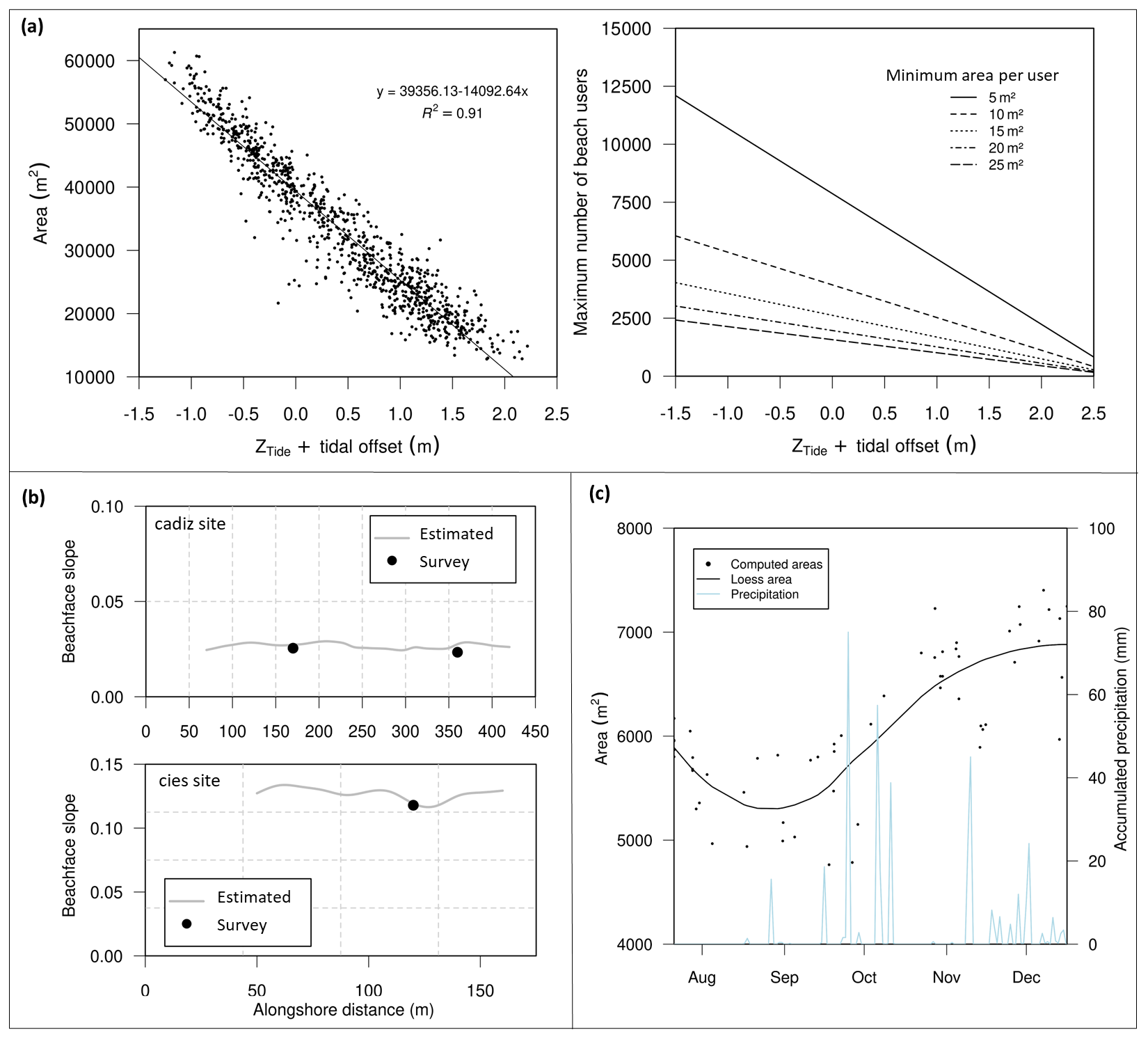
Figure 9 (a) Relationship between the tide and the maximum number of beach users at Santa Maria beach (cadiz), considering various scenarios for the minimum area per user (see text for explanation). (b) Average beachface slope for the cadiz and cies sites, obtained from SCShores (estimated values) and measured in situ (survey). The slope derived from GPS RTK-GNSS measured profiles was computed by considering the cross-shore distance between the profiles' points at the same Z as the estimated elevation of the SCShores for each date. (c) Comparison of the computed area using SCShores from samarador and the monthly accumulated precipitation data from the closest AEMET meteorological station.

Figure 9a presents a proxy for the beach carrying capacity at the mesotidal beach of Santa María in Cádiz (cadiz CS), based on its widths at different tidal stages. By analysing the area between the shoreline and the promenade, the dataset enables the calculation of available beach space. The left side of Fig. 9a shows the linear regression analysis of the calculated area for each date with respect to the estimated tide. It is important to note that the area is calculated with a fixed reference baseline, but the shorelines do not cover the entire beach, as Table 4 indicated. Therefore, the displayed area represents approximately 75 % of the alongshore extent of the beach. By means of the relationship (equation) derived from this analysis, the right side of Fig. 9a presents the number of potential beach users, under the assumption of no beach bars, tidal terraces, or other limitations. The calculation depends on the “optimal conditions for bathers” or conditions imposed by measures like those related to COVID across predefined occupancy degrees of 5 to 25 m² per user in order to determine the maximum number of users (Murillo et al., 2023; Zacarias et al., 2011; Zielinski and Botero, 2020). It should be noted that these data can be used as input in more sophisticated studies on beach carrying capacity. By incorporating the sea level information measured by the tide gauge at any given moment, coastal managers can accurately estimate the approximate beach area and determine the maximum number of users at sites such as Cadiz, where significant variations are unlikely. This valuable insight will contribute to effective management and planning that optimizes the use of the beach resources while maintaining a safe and enjoyable environment for visitors.

Another application of the SCShores dataset is the estimation of the beachface slope (Fig. 9b), calculated as in Eq. (6). The beachface slope (steepness) is a fundamental parameter for coastal morphodynamic research, as it is related to different morphological characteristics and processes such as sand grain size, wave run-up elevation, and total swash excursion at the shoreline (Vos et al., 2020). In applications of this nature, it is crucial to take into account the provided performance metrics as a function of distance, as illustrated in Fig. 6, as the error in ΔXY will significantly impact the calculated slope. The case of Rodas beach (cies CS) presents the most complex or limiting scenario. It is worth noting the notable contrast in scale between the cadiz and cies CS sites (Fig. 9b). The former represents a typical dissipative beach, while the latter corresponds to a reflective beach.

$$\begin{array}{}\text{(5)}& \mathit{\beta }={\displaystyle \frac{\mathrm{\Delta }Z}{\mathrm{\Delta }XY}},\end{array}$$

where ΔZ represents the elevation difference between two shorelines on the same day (low and hight tide), and ΔXY represents the difference in cross-shore position between these two shorelines. It is assumed that the shoreline elevation remains constant along the entire shoreline when calculated using CoastSnap.

The last example shows the evolution of the area of S'Amarador beach computed for all available shorelines (Fig. 9c). As S'Amarador beach is a microtidal beach (recorded sea level elevations range from 0.07 to 0.37 cm in the dataset) and the beach landward limit for the computation of the beach area has been defined by the position of the dune foot, the area of the beach is modulated by the shoreline displacement. In this way, assuming negligible tidal effects, beach area can be considered a proxy for beach width. For mesotidal beaches, beach width can also be calculated, but it is necessary to consider the tidal range. This can be done either by considering similar tidal ranges or by referencing all shorelines to a common Z datum (Almonacid-Caballer et al., 2016) using the slope of the beachface, which can also be retrieved with the provided dataset, as shown in prior applications (Fig. 9b).

The evolution of the S'Amarador beach area with overlapped records of monthly accumulated precipitation (Fig. 9c) shows that significant rainfall events may favour beach accretion. The beach is linked to a ravine that can become active during torrential rainfall events, transporting sediment to the beach if the intensity and duration of the event are sufficient. This analysis contributes to the geomorphological knowledge of beach behaviour and demonstrates that the SCShores dataset can be complemented with other forcing drivers to understand the key parameters controlling changes in coastal evolution.

5 SCShores: usage recommendations

The dataset is presented in a user-friendly format to ease its importation into widely used geographical information system (GIS) software such as QGIS and ArcGIS. In QGIS, the GeoJSON file can be added to the Layers Panel either by dropping it from the Browser Panel or by double-clicking on the file. However, in the ArcGIS environment, the Data Interoperability extension is required and must be activated prior to use.

By importing the dataset into GIS software, end-users can take advantage of the powerful functionalities offered by these platforms to visualize, manipulate, and extract valuable insights from the shoreline data. GIS software provides tools for spatial analysis, data integration, and visualization, enabling users to examine the dataset in conjunction with other relevant geospatial information.

Additionally, the dataset can also be accessed programmatically (e.g. Python, R), allowing for seamless integration into custom software applications or research workflows. This programmable accessibility enables coastal researchers to incorporate the dataset into their own analysis pipelines and automate data processing tasks, and it facilitates the development of specialized tools and models.

6 Data availability

The SCShores v.1.0 dataset (González-Villanueva et al., 2023b), described in Sect. 2.3 of this article, is accessible via the Zenodo data repository at https://doi.org/10.5281/zenodo.8056415. This dataset serves as a starting point for storing future shorelines gathered through the CoastSnap initiative in Spanish territories and for disseminating them to the scientific community and end-users. The authors will periodically update the database as new data from in situ shorelines measured with GPS RTK-GNSS become available for the validation process. New versions of SCShores will be uploaded to Zenodo, utilizing the repository's versioning feature.

7 Code availability

The source code used to rectify and map shorelines derived from crowdsourced smartphone images (CoastSnap) is available at https://github.com/Coastal-Imaging-Research-Network/CoastSnap-Toolbox (last access: 10 April 2023) and the technical methodology is described in Harley et al. (2019).

8 Conclusions

This study presents a novel dataset of shorelines derived from a citizen science initiative known as CoastSnap. The dataset focuses on five Spanish beaches spanning both meso- and microtidal environments and encompasses a comprehensive collection of 1721 shorelines, each represented by a multipoint feature with a regular spacing of 3 m. Notably, an assessment of the data quality reveals a compelling accuracy profile, with an estimated probability indicating that approximately 67 % of the measurements exhibit an error magnitude within 3 m, while 75 % of them demonstrate an error magnitude within 3.8 m.

The presented dataset provides invaluable insights into the local-scale variability of shoreline positions, serving as a unique and cost-effective resource for beach monitoring programmes, especially in regions where in situ observations are limited or unavailable. This dataset holds significant potential for various applications in coastal science and management, including:

• i.

  Estimating variability in beach width and area. The dataset allows for the estimation of beach width and area variations over time. This information is crucial for assessing beach carrying capacities and understanding beach evolution patterns.

• ii.

  Enhancing understanding of short- to medium-term coastal evolution. By analysing the dataset, researchers can gain a deeper understanding of the short-term coastal evolution processes and their relationships with driving forces such as wave action, sediment transport, and shoreline dynamics. This knowledge contributes to improved predictive models and more accurate coastal management strategies.

• iii.

  Estimating the beachface slope. The dataset enables the estimation of the beachface slope, a critical parameter required for multiple models used in coastal evolution studies. Accurate measurements of the beachface slope contribute to better modelling of sediment transport, beach nourishment projects, and erosion forecasting.

The utilization of this dataset in the above applications enhances the understanding of coastal dynamics and facilitates informed decision-making in coastal planning and conservation efforts. It presents a valuable tool for researchers, coastal engineers, and policymakers to address the challenges associated with coastal evolution and sustainable coastal zone management.

The dataset is conveniently available in a user-friendly format, making it easily importable into commonly used geographical information system (GIS) software. The dataset is accessible through both GIS software and programmable interfaces, which gives coastal researchers and end-users the flexibility and convenience to exploit the data in a manner that best suits their specific requirements.