Spatiotemporally consistent global dataset of the GIMMS Normalized Difference Vegetation Index (PKU GIMMS NDVI) from 1982 to 2022

Global products of remote sensing Normalized Difference Vegetation Index (NDVI) are critical to assessing the vegetation dynamic and its impacts and feedbacks on climate change from local to global scales. The previous versions of the Global Inventory Modeling and Mapping Studies (GIMMS) NDVI product derived from the Advanced Very High Resolution Radiometer (AVHRR) provide global biweekly NDVI data starting from the 1980s, being a reliable long-term NDVI time series that has been widely applied in Earth and environmental sciences. However, the GIMMS NDVI products have several limitations (e.g., orbital drift and sensor degradation) and cannot provide continuous data for the future. In this study, we presented a machine learning model that employed massive high-quality global Landsat NDVI samples and a data consolidation method to generate a new version of the GIMMS NDVI product, i.e., PKU GIMMS NDVI (1982–2022), based on AVHRR and Moderate-Resolution Imaging Spectroradiometer (MODIS) data. A total of 3.6 million Landsat NDVI samples that were well spread across the globe were extracted for vegetation biomes in all seasons. The PKU GIMMS NDVI exhibits higher accuracy than its predecessor (GIMMS NDVI3g) in terms of R² (0.97 over 0.94), root mean squared error (RMSE: 0.05 over 0.09), mean absolute error (MAE: 0.03 over 0.07), and mean absolute percentage error (MAPE: 9 % over 20 %). Notably, PKU GIMMS NDVI effectively eliminates the evident orbital drift and sensor degradation effects in tropical areas. The consolidated PKU GIMMS NDVI has a high consistency with MODIS NDVI in terms of pixel value (R² = 0.956, RMSE = 0.048, MAE = 0.034, and MAPE = 6.0 %) and global vegetation trend ($\mathrm{0.9}\times {\mathrm{10}}^{-\mathrm{3}}$ yr⁻¹). The PKU GIMMS NDVI product can potentially provide a more solid data basis for global change studies. The theoretical framework that employs Landsat data samples can facilitate the generation of remote sensing products for other land surface parameters. The PKU GIMMS NDVI product is open access and available under a Creative Commons Attribution 4.0 License at https://doi.org/10.5281/zenodo.8253971 (Li et al., 2023).

1 Introduction

The Normalized Difference Vegetation Index (NDVI) characterizes the biophysical, biochemical, and physiological conditions of vegetation (Rouse et al., 1974; Rondeaux et al., 1996; Gao et al., 2000; Yin et al., 2022). As a normalized ratio of the near-infrared (NIR) and red bands, it minimizes many forms of multiplicative noise, including soil background, atmosphere, and sun–target–sensor geometry (Rondeaux et al., 1996; Gao et al., 2000; Yin et al., 2022). Due to its long archive, simplicity, and robustness, NDVI is one of the most popular vegetation indices (VIs) that have been widely used in the quantification of vegetation dynamics (Badgley et al., 2017; Gamon et al., 2016; Joiner et al., 2018; Li et al., 2019), terrestrial carbon and water cycles (Zhu et al., 2021; Wang et al., 2021; Schubert et al., 2012; Cui et al., 2021), and environmental stress and disturbances (AghaKouchak et al., 2015; Qin et al., 2021; Peng et al., 2020). The NDVI has been acquired from satellite sensors since the 1970s, but it was not until the late 1990s that NDVI data of different temporal and spatial resolutions became steadily available from better designed and calibrated sensors such as the Moderate-Resolution Imaging Spectroradiometer (MODIS) (Didan, 2021), “Satellite Pour l'Observation de la Terre” (SPOT) VEGETATION (SPOT-VGT) (Maisongrande et al., 2004), and Visible Infrared Imaging Radiometer (VIIRS) (Cao et al., 2014). For a long time before the late 1990s, the Advanced Very High Resolution Radiometer (AVHRR) sensor on board NOAA satellites had been the only NDVI data source that provided frequent and continuous global observations. Several sets of global long-term time-series NDVI products have been released based on AVHRR, such as the Global Inventory Modeling and Mapping Studies (GIMMS) NDVI3g (Pinzon and Tucker, 2014), Long Term Data Record version 4 (LTDR4) NDVI (Pedelty et al., 2007), and Vegetation Index and Phenology version 3 (VIP3) NDVI (Pedelty et al., 2007). These products have provided great insights into how ecological processes of vegetation influence and respond to ongoing climate change (Wang et al., 2021; Zhu et al., 2021; Zhang et al., 2017; Piao et al., 2020; Myers-Smith et al., 2020; Chen et al., 2019). However, uncertainties in the NDVI products have also led to inconsistency not only between different products but also for the same product in different periods, placing many studies in a dilemma, particularly when characterizing long-term changes (Wang et al., 2022; Zeng et al., 2022; Fensholt and Proud, 2012; Shen et al., 2022).

There are several sources of uncertainties in AVHRR-based NDVI products. The first comes from the discrepancies in band settings (e.g., center wavelength and spectral response function) within AVHRR sensors (i.e., AVHRR-2 and AVHRR-3) as well as with other sensors (such as MODIS and VIIRS) (Yang et al., 2021; Trishchenko et al., 2002; Pinzon and Tucker, 2014; Fan and Liu, 2016). Second, NDVI inconsistencies could also occur between the same AVHRR sensors on board different NOAA satellites. In this case, the sensors would have different image acquisition times and sun–target–sensor geometries, yielding a “jump” (a sudden change in values) phenomenon in the NDVI time series (Tian et al., 2015; Frankenberg et al., 2021; Jiang et al., 2017; Los, 1998). For example, the AVHRR sensor on board NOAA-11 has a considerably larger NDVI than preceding and subsequent AVHRR sensors (Beurs and Henebry, 2004). Third, uncertainties could be introduced by the NOAA satellite orbital drift and AVHRR sensor degradation due to the harsh environments in space (Wang et al., 2022). Artificial signals from the orbital drift in humid areas were evident for the AVHRR-based NDVI products (e.g., VIP3 NDVI, LTDR4 NDVI, and GIMMS NDVI3g) and downstream products such as the GIMMS Leaf Area Index (LAI3g) (Zhu et al., 2013).

For long-term vegetation trend analysis, an accurate global NDVI product requires us to address the abovementioned uncertainties well, particularly the ones related to temporal inconsistency. Some efforts have thus been made in past years (Tucker et al., 2005; Jiang et al., 2008; Doelling et al., 2007; Cao et al., 2004). One strategy performed NDVI calibration using the data acquired when NOAA orbital drift or AVHRR sensor degradation had not occurred. For example, Jiang et al. (2008) used NDVI in the inaugural year of NOAA satellites as a baseline to calibrate NDVI of other years. The other strategy calibrated AVHRR NDVI with other sensors with overlapping observation periods with AVHRR. Pinzon and Tucker (2014) used SeaWiFS NDVI data as a benchmark to evaluate the consistency of GIMMS NDVIg data with a Bayesian approach. Other studies have employed SPOT-VGT NDVI data (Tucker et al., 2005), Meteosat-8 NDVI data (Doelling et al., 2007), MODIS NDVI data (Cao et al., 2004), or VIIRS data (Yang et al., 2021) to calibrate the other NDVI products derived from AVHRR sensors. The basic assumption behind the two strategies is that the calibration models and parameters derived from one or more overlapping periods must be static through time. This is not necessarily true because the performance of satellite sensors could be a function of multiple factors that are not limited to their internal settings and seasonality (Kogan, 1995). Without a sufficient understanding of product accuracy in all periods, uncertainties in AVHRR NDVI calibration can hardly be determined.

The Landsat data have the potential to evaluate and calibrate global NDVI products in all periods. As one of the earliest satellite missions, Landsat satellite series have provided the longest space-based record of Earth's land since the 1970s (Roy et al., 2016; Wulder et al., 2019, 2016). Landsat sensors have a high spatial resolution; low frequencies of sensor change; and, in particular, high accuracy and consistency in geometric and radiometric properties (Zhang et al., 2021; Weng et al., 2014; Dong et al., 2020; Storey et al., 2014). Verification results from pseudo-invariant calibration sites (PICS) (such as desert, water, ice, and snow) showed that the temporal variations of top-of-atmosphere (TOA) reflectance were less than 2 % for most Landsat sensors (except for Landsat 5 TM at SWIR 2 which is 3 %) during their orbit time (Helder et al., 2013). Although the relatively small field of view and long revisit period have limited Landsat for global applications (Maisongrande et al., 2004), its excellent temporal consistency has aided some important studies of vegetation trend via sample analysis, such as in the Arctic region from 1984 to 2016 (Berner et al., 2020). In recent years, an increasing number of studies have used Landsat data for global dataset production via tools such as the Google Earth Engine (GEE) platform (Zhang et al., 2022; Cao et al., 2021).

In this context, this study uses long-term Landsat data to develop a new version of the GIMMS NDVI product (PKU GIMMS NDVI) (1982–2022) from the GIMMS NDVI3g (current version) (1982–2015) and MODIS NDVI products (2003–2022). We first cross-calibrate NDVI data from different Landsat missions and extract a mass of high-quality Landsat NDVI samples worldwide for all periods (1984–2015). Based on the samples, we generate the PKU GIMMS NDVI using biome-specific back-propagation neural network (BPNN) models with GIMMS NDVI3g data and selected explanatory variables (the longitude and latitude, associated month, and the NOAA number and years since launch). Then, the temporal coverage of PKU GIMMS NDVI is extended to the year 2022 by consolidating with the MODIS NDVI product using a pixel-by-pixel random forest (RF) regression method. Results of Landsat NDVI cross-calibration are reported. We directly validate PKU GIMMS NDVI's accuracy via independent Landsat NDVI samples and compare it with GIMMS NDVI3g. We also examine the accuracy distribution in space for both products and demonstrate the performance of PKU GIMMS NDVI in alleviating uncertainties from the orbital drift and sensor degradation. The consolidation of PKU GIMMS NDVI with MODIS NDVI and the performance of consolidated PKU GIMMS NDVI in characterizing vegetation trends are also evaluated.

2 Data

Four global satellite products were used in this study: Landsat Surface Reflectance data (Collection 1 Tier 1) (Masek et al., 2006; Vermote et al., 2016), the MODIS Land Cover Type product (V6.1) (Friedl et al., 2002), the GIMMS NDVI3g product (V1.0) (Pinzon and Tucker, 2014), and the MODIS NDVI product (V6.1) (Didan, 2021). The Landsat Surface Reflectance data were used to generate NDVI samples. The MODIS Land Cover Type product was used to label NDVI samples with vegetation biome types. The GIMMS NDVI3g product was the main data source from which our PKU GIMMS NDVI product would be created. The MODIS NDVI product was used to extend the temporal coverage of the generated PKU GIMMS NDVI product.

2.1 Landsat Surface Reflectance data (Collection 1 Tier 1)

We obtained Landsat Surface Reflectance data between 1984 and 2015 with a spatial resolution of 30 m from the GEE platform. These data comprised the Collection 1 (Tier 1) datasets of Landsat 5 (TM), 7 (ETM+), and 8 (OLI), produced by the United States Geological Survey (USGS). Landsat 5 was launched in March 1984 and retired in January 2013. Landsat 7 and 8 were launched in April 1999 and February 2013, respectively, and are still in operation. The USGS uses the Landsat Ecosystem Disturbance Adaptive Processing System (Masek et al., 2006) to perform atmospheric and terrain corrections for Landsat 5 and Landsat 7 and uses the Landsat 8 Surface Reflection code (Vermote et al., 2016) to perform corrections for Landsat 8. Previous studies have revealed that Landsat reflectance data have good temporal consistency that can be used to produce a set of long-term stable benchmarks (Helder et al., 2013). However, this study found a systematic deviation between Landsat 5/Landsat 8 and Landsat 7. The correction method for the systematic deviation is described in Sect. 3.1.

2.2 GIMMS NDVI3g (V1.0) product

This study selected the latest version (third generation) of the GIMMS NDVI dataset (GIMMS NDVI3g, V1.0) generated from AVHRR sensors on board a series of NOAA satellites (NOAA 7, 9, 11, 14, 16, 17, and 18) (Pinzon and Tucker, 2014). The GIMMS NDVI3g dataset has a spatial resolution of $\mathrm{1}/\mathrm{12}$^∘. A half-month maximum NDVI composite was used to eliminate the atmospheric effects on the NDVI magnitude. This compositing scheme resulted in two maximum NDVI values per month. The GIMMS NDVI3g record extending from January 1982 to December 2015 was used in this study. Pixels with negative NDVI values that referred to snow and other contaminated data (e.g., pixels with large inland water bodies) and pixels of bad quality, determined by the quality control (QC) layer, were removed from all analyses.

2.3 MODIS Vegetation Index product (MOD13C1, V6.1)

The MODIS Vegetation Index product (MOD13C1) (Didan, 2021) is accessible at NASA's Earth Observing System Data and Information System (EOSDIS) (https://search.earthdata.nasa.gov/, last access: September 2023). Compared to old versions, the latest MOD13C1 version 6.1 provides several algorithmic improvements and corrects the sensor degradation effect well (Zhang et al., 2017). As the MODIS NDVI product was used to consolidate with PKU GIMMS NDVI, we chose MOD13C1 over other MODIS Vegetation Index products because it was derived from MODIS Terra, which has been available since 2000 and has a close temporal (16 d) and spatial resolution (0.05^∘) compared to those of PKU GIMMS NDVI (half-month and $\mathrm{1}/\mathrm{12}$^∘). This study employed the year-round global MOD13C1 during 2003–2022. MOD13C1 provides a pixel reliability layer that distinguishes good-quality data from no data, marginal data, snow/ice, and cloudy and estimated data. To match the temporal and spatial resolutions, we first performed a time-weighted aggregation method on MOD13C1 to produce an NDVI product at a temporal resolution of half-month. The method was adopted from Zhu et al. (2013). Its central idea is to assign weights to all MOD13C1 scenes that could temporally intersect with a particular half-month interval, where the weight depends on the possibility of intersection. The half-month NDVI product was finally calculated as the weighted sum of the scenes. We then performed nearest-neighbor sampling to upscale the spatial resolution to $\mathrm{1}/\mathrm{12}$^∘.

2.4 MODIS Land Cover Type products (MCD12Q1 and MCD12C1, V6.1)

The MODIS Land Cover Type products provide global maps of land cover for each year between 2001–2019 (Friedl et al., 2002). It has five legacy classification schemes, including the International Geosphere-Biosphere Programme (IGBP) classification system, the University of Maryland (UMD) classification system, the Leaf Area Index (LAI) classification system, the Biome-BGC (biogeochemical cycle) classification system, the plant functional type (PFT) classification system, and the FAO Land Cover Classification System (LCCS) classification system. The LAI classification scheme was used in this study. The LAI classification scheme has 11 classes, including eight natural vegetation types (evergreen needleleaf forests (ENF), evergreen broadleaf forests (EBF), deciduous needleleaf forests (DNF), deciduous broadleaf forests (DBF), shrublands (SHR), savannas (SAV), grasslands (GRA), croplands (CRO)) and three non-vegetated lands (water bodies (WAT), non-vegetated lands (NVG), and urban and built-up lands (URB)). In data analysis, we also merged the natural vegetation types into one global vegetation biome (GLO). This study employed two MODIS Land Cover Type products with different spatial resolutions, i.e., 500 m (MCD12Q1; Friedl and Sulla-Menashe, 2022a) and 0.05^∘ (MCD12C1; Friedl and Sulla-Menashe, 2022b). The MCD12Q1 was used to select sample locations for Landsat NDVI cross-calibration (Sect. 3.1.1). The MCD12C1 was used to establish biome-specific BPNN models with GIMMS NDVI3g after being spatially aggregated to $\mathrm{1}/\mathrm{12}$^∘ using the nearest-neighbor resampling method (Sect. 3.2.2). The vegetation biome type with the highest frequency from 2001–2019 was considered the vegetation biome type from 1982–2022. This could be a margin of error, but it is the best option.

Figure 1 Schematic diagram of the generation and evaluation of the PKU GIMMS NDVI product.

3 Methodology

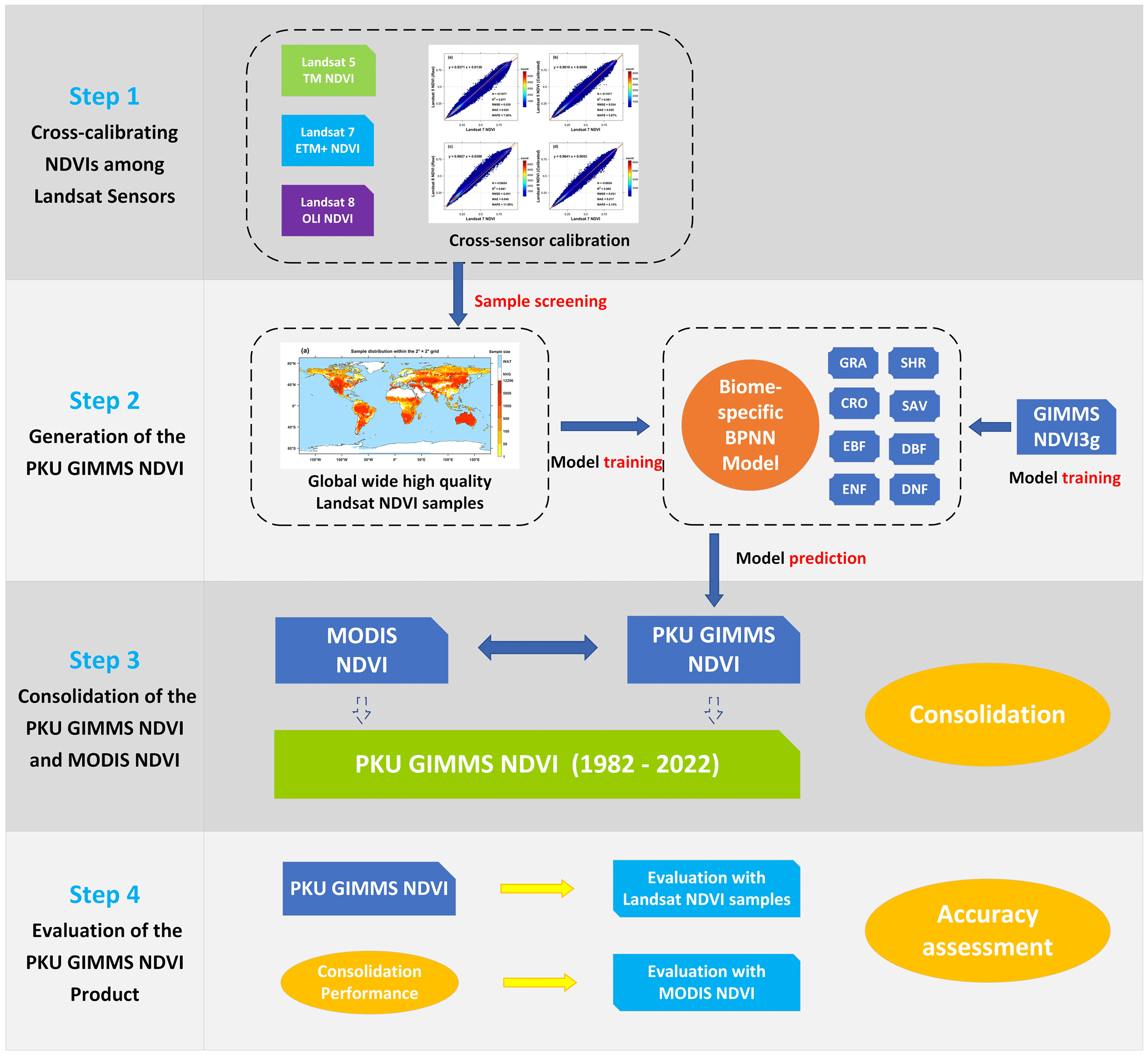
A schematic overview of the methodology involves four key steps as illustrated in Fig. 1: (1) Landsat sensor cross-calibration to create temporally consistent Landsat data as a benchmark; (2) generation of PKU GIMMS NDVI from GIMMS NDVI3g using per-biome Landsat NDVI samples, BPNN models, and other explanatory variables; (3) consolidation of PKU GIMMS NDVI with MODIS NDVI to extend the temporal coverage of PKU GIMMS NDVI to the year 2022; and (4) evaluation of PKU GIMMS NDVI in terms of its performance in temporal and spatial accuracies and in eliminating the orbital drift and sensor degradation.

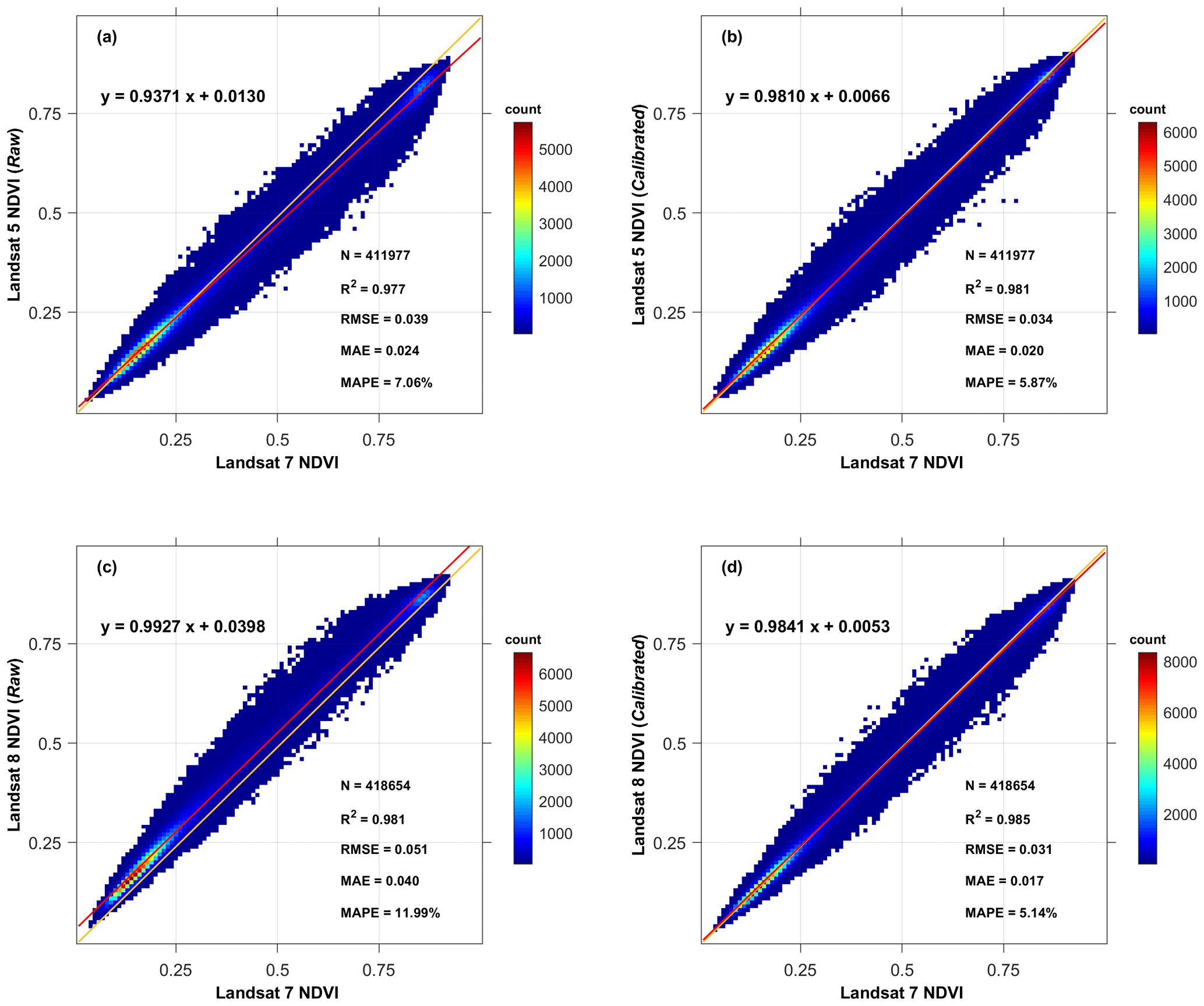
Figure 2 The efficiency of NDVI cross-calibration between Landsat sensors. (a) Landsat 7 NDVI vs. uncalibrated Landsat 5 NDVI. (b) Landsat 7 NDVI vs. calibrated Landsat 5 NDVI. (c) Landsat 7 NDVI vs. uncalibrated Landsat 8 NDVI. (d) Landsat 7 NDVI vs. calibrated Landsat 8 NDVI. The red line is the regression line, and the diagonal orange line represents a 1:1 relationship. The size of the NDVI interval in the maps is 0.01. NDVI intervals with sample number <10 were omitted.

3.1 Cross-calibrating NDVIs among Landsat sensors

Systematic deviation exists in the NDVI between Landsat 5, Landsat 7, and Landsat 8 (Berner et al., 2020). Specifically, the NDVI derived from Landsat 5 is smaller than that from Landsat 7, and the NDVI from Landsat 7 is smaller than that of Landsat 8 (Berner et al., 2020) (Fig. 2a and c). The systematic deviations were first removed as the Landsat NDVI served as a benchmark in this study. We adopted the method by Berner et al. (2020) that used BPNN to calibrate Landsat 5 and Landsat 8 to the Landsat 7 level. The reason for considering Landsat 7 as the benchmark is that Landsat 7 has overlapping periods with both Landsat 5 and Landsat 8.

3.1.1 Sample locations

For the Landsat sensor cross-calibration, 100 000 sample locations were randomly selected for each vegetation biome type from the MCD12Q1. For each sample (500 m resolution), a matrix of 20×20 Landsat pixels (30 m resolution) was extracted at the sample center from Landsat 5, Landsat 7, and Landsat 8 images acquired between 1984 and 2015. The Landsat pixels at each sample location were further refined to guarantee that only high-quality clear-sky measurements were included in our study.

First, all Landsat data during August 1991 and December 1992 when Mount Pinatubo erupted were excluded. Second, the abundance of aerosols and thin clouds was used to determine the quality of the sample location (and associated Landsat pixels). If many of the pixels had a high atmospheric opacity (provided by Landsat products), the whole sample location was removed. For Landsat 5 and Landsat 7, the threshold of average atmospheric opacity was set to 0.3. For Landsat 8, the percentage of clear pixels (which have an atmospheric opacity index of 1) must be higher than 80 % (320 pixels). Third, the quality of the Landsat scene, the cloud contamination, and the radiation magnitude were used to determine the quality of individual pixels. A pixel was marked as low-quality if (1) the associated Landsat scene had excessive cloud coverage (>80 %); (2) the pixel was contaminated by clouds, cloud shadows, water, or snow judged by the CF Mask algorithm (Foga et al., 2017; Zhu et al., 2015); or (3) the pixel had implausibly high (>1) or extremely low (0.001) surface reflectance due to radiation saturation and atmospheric adjustment. This study removed the whole sample location if the percentage of high-quality pixels was lower than 90 % (360 pixels).

NDVI was calculated and averaged from high-quality pixels at the remaining sample locations. The sample locations were divided into 80 % for model training and 20 % for model evaluation.

3.1.2 Cross-calibration using BPNN models

BPNN is one of the most popular and established artificial neural network (ANN) algorithms used in ecological studies (Hong et al., 2021; Meng et al., 2020; Yang et al., 2018). An ANN is a machine learning algorithm inspired by the structure and function of biological neural networks. A typical ANN comprises input (explanatory variables), output (target variable), and hidden layers, each containing artificial neurons whose numbers range from several to hundreds. In the model training of BPNN, signals flow from the input layer to the output layer, after likely passing through several hidden layers. Errors in the output layer propagate backward to the previous layers until they satisfy the user-defined threshold, and the network attempts to minimize the discrepancies between observations and predictions.

This study used NDVI sample locations (500 m resolution) in the overlapping periods between Landsat 7 and Landsat 5/Landsat 8 to train BPNN models. The models were then extrapolated to calibrate Landsat 5 and Landsat 8 in non-overlapping periods. The extrapolation to non-overlapping periods was reliable on the basis that the optical sensors on board Landsat satellites are temporally consistent with themselves, and the reflectance data have been geometrically and radiometrically calibrated well (Irons et al., 2012; Wulder et al., 2019, 2016). Specifically, NDVI values from Landsat 7 and Landsat 5/Landsat 8 were paired at each sample location (Sect. 3.1.1) if their acquisition times were less than 10 d. In total, 12 718 863 sample pairs were obtained for all vegetation biome types. When training the BPNN model, the NDVI of Landsat 5/Landsat 8 was used as the explanatory variable, and the NDVI of Landsat 7 was the target variable. We also included the image acquisition time (day of the year) and the sample location's spatial coordinates (longitude and latitude) as covariates to explain potential seasonal and regional variations in the samples.

3.2 Generation of the PKU GIMMS NDVI

3.2.1 Landsat NDVI samples

The cross-calibrated Landsat data were used to calibrate the GIMMS NDVI3g product. Landsat data are known for their unparalleled radiometric and geometric accuracy and stability, as well as their longest continuity, global coverage, and relatively high spatial resolution (Wulder et al., 2019, 2016). A total of 40 000 sample locations were randomly selected from the GIMMS NDVI3g product with a spatial resolution of $\mathrm{1}/\mathrm{12}$^∘. Then at a time step of half-month, we identified sample locations with high-quality GIMMS NDVI3g data (QC = 0) and uniformly placed 9 matrices of 20×20 Landsat pixels within each location ($\mathrm{1}/\mathrm{12}$^∘). Landsat pixel values were extracted from all available scenes. Their quality was examined in the same way as Sect. 3.1.1. We removed all matrices whose proportion of high-quality pixels <90 % (360 pixels). The sample locations at a particular time were treated as Landsat NDVI samples if more than half (i.e. > = 5) of nine matrices remained. The sample value was calculated as the average NDVI from high-quality Landsat pixels. The samples were also divided into 80 % for model training and 20 % for NDVI product evaluation.

3.2.2 BPNN models with GIMMS NDVI3g and other explanatory variables

With the Landsat NDVI samples ($\mathrm{1}/\mathrm{12}$^∘ resolution), the BPNN model was also used to calibrate the GIMMS NDVI3g product. In the BPNN model, GIMMS NDVI3g data from 1984 to 2015 were used as an explanatory variable, and the Landsat NDVI was the target variable. We also included other explanatory variables associated with spatial, temporal, and satellite information. The spatial information (longitude and latitude) accounts for the spatial autocorrelation in image samples, temporal information (month) accounts for vegetation dynamics, and satellite information (NOAA satellite number and years since its launch) accounts for issues from NOAA orbit drift and AVHRR sensor degradation. One BPNN model was built for each of the eight vegetation biome types. GIMMS NDVI3g was first explored as a single explanatory variable in the BPNN model, and other explanatory variables were added in an enumerative order. In detail, five feature combinations were set up to evaluate their impacts on the BPNN model: (S1) NDVI alone; (S2) NDVI and spatial information (longitude and latitude); (S3) NDVI, spatial information, and time information (month); (S4) NDVI, spatial information, time information, and NOAA satellite number; and (S5) NDVI, spatial information, time information, NOAA satellite number, and years since its launch. The optimal parameters for each enumeration were derived through 10-fold cross-verification. The final BPNN model for NDVI calibration was determined with an appropriate set of explanatory variables and the optimal parameters.

3.3 Consolidation of the PKU GIMMS NDVI and MODIS NDVI

Over the past 2 decades, GIMMS NDVI3g products have been extensively utilized for spatiotemporal dynamic monitoring of vegetation, carbon and water cycles of ecosystems, and other related studies. They have provided powerful data support for several significant conclusions in Earth and environmental sciences. However, the latest data in GIMMS NDVI3g is until 2015 and no further upgrades will be provided. This study extended the temporal coverage of GIMMS NDVI3g so that the investigation of recent responses and feedback of vegetation to climate change can be possible. The MODIS NDVI product has excellent precision, temporal consistency, and a long-time span. It is considered the best medium–high resolution global NDVI produced over the past 2 decades. It could be utilized as an effective extension of the PKU GIMMS NDVI.

However, the band settings of MODIS are different from that of AVHRR. A simple combination of these two products would lead to systematic inconsistencies in NDVI values. Some methods have been proposed to deal with this issue, such as maximum–minimum stretching (Yang et al., 2021), histogram matching (Jiang et al., 2008), and machine learning (Berner et al., 2020). In this study, we used a pixel-wise method inspired by Mao et al. (2012) to splice the PKU GIMMS NDVI product (1982–2015) and MODIS NDVI product (2003–2022). The pixel-wised method has been demonstrated more accurate than the global models (Yang et al., 2021). Specifically, the MODIS NDVI was first resampled to have the same spatial resolution ($\mathrm{1}/\mathrm{12}$^∘) and temporal resolution (half a month) as the PKU GIMMS NDVI (see Sect. 2.3). Then, during the overlapping periods (2003–2015), an 11×11 moving window (approximately 1^∘ equivalent) was placed around each pixel. All the same vegetation biome type with the pixel were identified, and their NDVI values were extracted from both products. This resulted in at most 1573 GIMMS-MODIS NDVI sample pairs (11×11 pixels per year in 13 years) for each pixel location. The sample pairs were further screened based on the data quality of PKU GIMMS NDVI (quality information adopted from GIMMS NDVI3g; see Sect. 2.2) and MODIS NDVI (see Sect. 2.3). Based on the sample pairs, the RF regression model was constructed (Breiman, 2001), with explanatory variables of the PKU GIMMS NDVI and the longitude and latitude of samples and target variable of the MODIS NDVI. This study found that the significance of the RF model largely depended on the data quality of PKU GIMMS NDVI and MODIS NDVI. As such, we used 90 % of the sample pairs for RF establishment and 10 % for validation. R² was calculated. The pixel-wise RF model was applied to the non-overlapping period only when R²>0.2 with p<0.001; otherwise, the PKU GIMMS NDVI was adjusted by aligning its mean value to that of the MODIS NDVI. The final PKU GIMMS NDVI product comprised the NDVI product derived from GIMMS NDVI3g between 1982 and 2002 and the MODIS NDVI product between 2003 and 2022.

3.4 Evaluation of the PKU GIMMS NDVI product

This study used a direct verification method to evaluate our product of PKU GIMMS NDVI (Justice et al., 2000). The PKU GIMMS NDVI (before consolidation) product was compared to Landsat NDVI values at the remaining 20 % of the sample locations ($\mathrm{1}/\mathrm{12}$^∘) for different vegetation biome types. As a comparison, the GIMMS NDVI3g was evaluated in the same manner. Four metrics were calculated for accuracy assessment, i.e., sample number (N), R², root mean square error (RMSE), mean absolute error (MAE), and mean absolute percentage error (MAPE). R² measures the percentage of variations that models can explain, RMSE measures the variance of errors, and MAE and MAPE measure absolute and relative error values at the sample level.

$$\begin{array}{}\text{(1)}& {\displaystyle }{R}^{\mathrm{2}}=\mathrm{1}-{\displaystyle \frac{\sum _{i=\mathrm{1}}^N({\text{NDVI}}_{\mathrm{Landsat}}-{\text{NDVI}}_{\mathrm{GIMMS}}{)}^{\mathrm{2}}}{\sum _{i=\mathrm{1}}^N({\text{NDVI}}_{\mathrm{Landsat}}-\stackrel{\mathrm{‾}}{{\text{NDVI}}_{\mathrm{Landsat}}}{)}^{\mathrm{2}}}}\text{(2)}& {\displaystyle }\text{RMSE}=\sqrt[\mathrm{2}]{{\displaystyle \frac{{\sum }_{i=\mathrm{1}}^n({\text{NDVI}}_{\mathrm{Landsat}}-{\text{NDVI}}_{\mathrm{GIMMS}}{)}^{\mathrm{2}}}{N}}}\text{(3)}& {\displaystyle }\text{MAE}={\displaystyle \frac{\mathrm{1}}{N}}\sum _{i=\mathrm{1}}^N\left|{\text{NDVI}}_{\mathrm{Landsat}}-{\text{NDVI}}_{\mathrm{GIMMS}}\right|\text{(4)}& {\displaystyle }\mathrm{\text{MAPE}}\mathit{\%}={\displaystyle \frac{\mathrm{1}}{N}}\sum _{i=\mathrm{1}}^N\left|{\displaystyle \frac{{\text{NDVI}}_{\mathrm{Landsat}}-{\text{NDVI}}_{\mathrm{GIMMS}}}{{\text{NDVI}}_{\mathrm{Landsat}}}}\right|\times \mathrm{100}\mathit{\%}\end{array}$$

The spatial distribution of R² was analyzed for the PKU GIMMS NDVI and GIMMS NDVI3g products in 2^∘ × 2^∘ grids. To highlight the differences between AVHRR-2 and AVHRR-3, NDVI products were evaluated in two separate periods (AVHRR-2: 1982–2000 and AVHRR-3: 2001–2015).

We also evaluated the performance of our PKU GIMMS NDVI (before consolidation) product in alleviating the effects of orbital drift and sensor degradation and compared it to the GIMMS NDVI3g product. Tian et al. (2015) observed that the GIMMS NDVI3g product showed a noticeable artefact in humid areas, which may have been caused by the NOAA satellite orbit drift and AVHRR sensor degradation. Zhu et al. (2013) also documented the significant orbital drift in the tropics. However, their conclusions either lacked a quantitative analysis or were solely based on statistical observations at a regional scale because long-term, continuous, and time-consistent benchmark data before 2000 were lacking. This study used NDVI bias in the tropical vegetation type of EBF to measure the magnitude of the orbital drift and sensor degradation effect. The bias was calculated as the mean value of NDVI deviation relative to Landsat NDVI in percentage (Helder et al., 2013) (Eq. 5).

$$\begin{array}{}\text{(5)}& \text{bias}\mathit{\%}={\displaystyle \frac{\mathrm{1}}{N}}\sum _{i=\mathrm{1}}^N{\displaystyle \frac{({\text{NDVI}}_{\mathrm{GIMMS}}-{\text{NDVI}}_{\mathrm{Landsat}})}{{\text{NDVI}}_{\mathrm{Landsat}}}}\times \mathrm{100}\mathit{\%}\end{array}$$

If there is orbital drift or sensor degradation, the bias will drastically fluctuate; otherwise, it remains constant. Seasonal fluctuations in the time series of NDVI bias were first removed by subtracting the multi-year average at a particular time of the year, i.e.,

$$\begin{array}{}\text{(6)}& {\text{bias\_deseason}}_{y,t}={\text{bias\_origin}}_{y,t}-\text{mean}\left({\text{bias\_origin}}_t\right),\end{array}$$

where bias_origin_y,t is the original NDVI bias at the time t of the year y (e.g., the first half-month of January in 2005), mean(bias_origin_t) is the multi-year average at the time t (e.g., the first half-month of January for all years), and bias_deseason_y,t is the NDVI bias after removing the seasonal fluctuation. Then, inter-annual trends of the bias were extracted via the ensemble empirical mode decomposition (EEMD) approach (Huang et al., 1998).

The consolidation of PKU GIMMS NDVI with MODIS NDVI was evaluated at 1000 random points for each vegetation biome type. Using MODIS NDVI as the reference, R², RMSE, MAE, MAPE, and bias for PKU GIMMS NDVI before and after consolidation were calculated and compared during the overlap period (2003–2015). To evaluate the performance of PKU GIMMS NDVI in characterizing vegetation trends (greening or browning), we performed linear regression analysis on the time series of annual average NDVI at each pixel. The linear regression slope could represent a green trend (positive slope value) or a browning trend (negative slope value). Trends from multiple NDVI products, i.e., GIMMS NDVI3g, MODIS NDVI, and PKU GIMMS NDVI (before and after consolidation), were compared over their overlapping period. The PKU GIMMS NDVI before consolidation was included because it represents the version of our NDVI product that is solely based on AVHRR data, and it can provide a more direct evaluation of the efficacy of the BPNN model and Landsat NDVI samples.

4 Results

4.1 Cross-calibration between Landsat 7 and Landsat 5/Landsat 8

More than 12 million Landsat sample pairs (600 m resolution) were acquired for Landsat sensor cross-calibration. Based on the samples, 16 BPNN models were established to calibrate Landsat 5 NDVI and Landsat 8 NDVI for eight vegetation biome types. Figure 2b and d show the NDVI calibration results of Landsat 5 and Landsat 8 against Landsat 7. Both relationships were strong with high R² (R²=0.981 for Landsat 5 and 0.985 for Landsat 8), low RMSE (RMSE = 0.034 for Landsat 5 and 0.031 for Landsat 8), low MAE (MAE = 0.020 for Landsat 5 and 0.017 for Landsat 8), and low MAPE (MAPE = 5.87 % for Landsat 5 and 5.14 % for Landsat 8). Compared to uncalibrated data (Fig. 2a and c), negative deviation in Landsat 5 NDVI and positive deviation in Landsat 8 NDVI have been efficiently eliminated.

4.2 The PKU GIMMS NDVI product

4.2.1 Spatiotemporal representativeness of the Landsat NDVI samples

Approximately 3.6 million Landsat NDVI samples ($\mathrm{1}/\mathrm{12}$^∘) from 1984 to 2015 were obtained for GIMMS NDVI3g calibration. The count and spatiotemporal distribution of the samples primarily depended on the availability of Landsat images, which were affected by clouds, cloud shadows, aerosols, climatic conditions, and other factors. The sample count per vegetation biome type was approximately proportional to its total area of coverage (Fig. 3a and b).

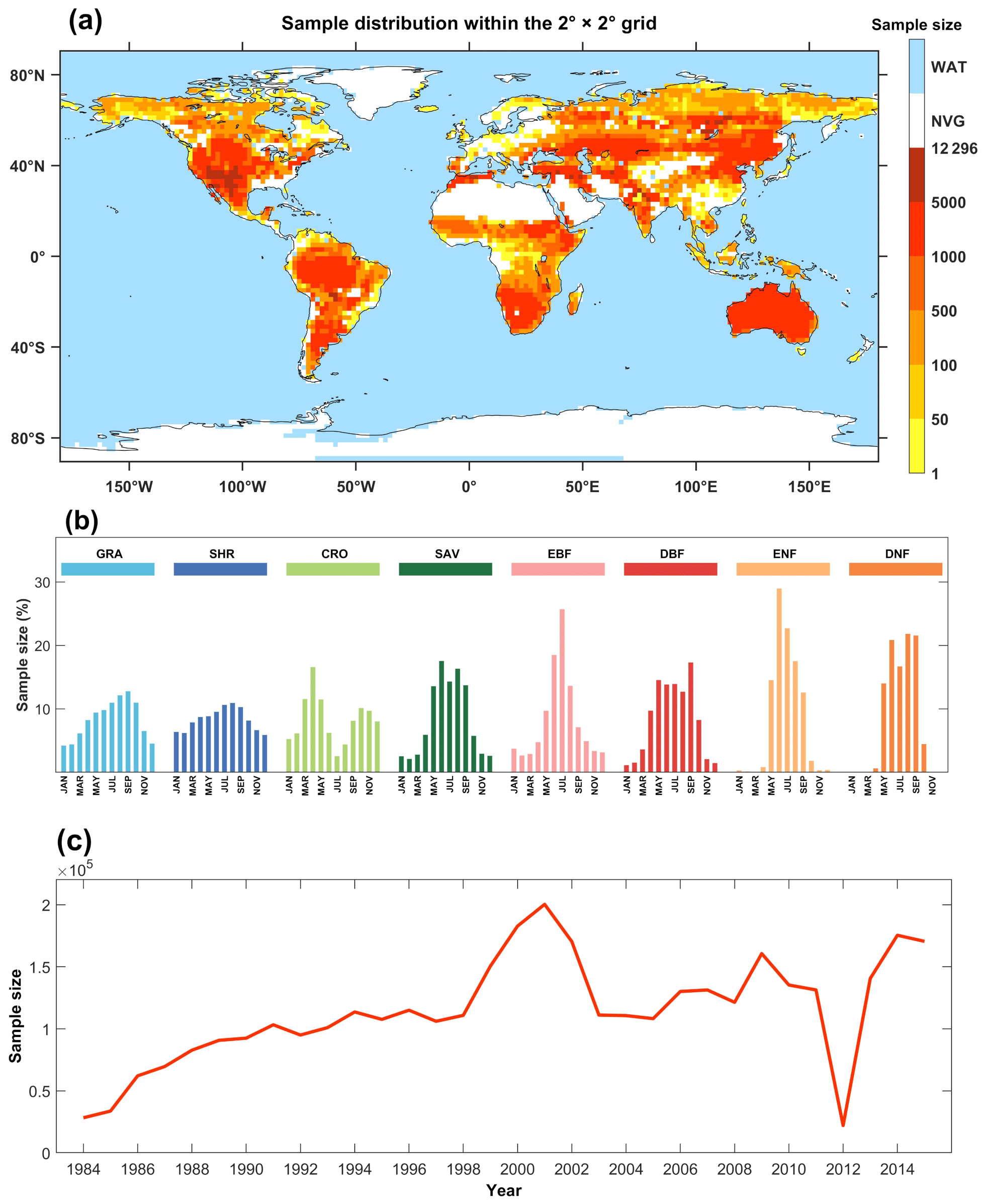
Figure 3 Spatial and temporal distribution of refined Landsat NDVI samples (3.6 million). (a) Distribution of Landsat NDVI samples within the 2^∘ × 2^∘ grid. (b) Percentage of samples among the eight vegetation biome types in each month. (c) Annual variation of Landsat NDVI sample size.

In the spatial domain, our samples covered most vegetated regions worldwide (Fig. 3a). Meanwhile, in some regions, the number of high-quality samples was relatively small. These regions include (1) northern high latitudes, which suffer from the polar night phenomenon, high solar zenith angle, and high observation zenith angle; (2) tropical rainforest areas with abundant precipitation and clouds which lower the quality of remote sensing data; and (3) the Sichuan Basin in southwest China and areas with a temperate marine climate (e.g., western European continent, British Isles, and west coast of North and South America). In the time domain (Fig. 3b), the samples of vegetation biome types showed single (for most biomes except CRO) or double (CRO) peaks depending on the time of their growing seasons. This guaranteed sufficient samples for accurate NDVI prediction with BPNN in the growing season. For the biomes of ENF and DNF that are primarily distributed in the high northern latitudes, the number of samples in winter (October to April) was <500. We resolved this problem by reducing the explanatory variables in the BPNN model. During 1984–2015, the Landsat NDVI sample size generally increased from Landsat 5 to Landsat 7 and Landsat 8 except for two periods. Between 1999 and 2003, the sample size was significantly larger as both Landsat 5 and Landsat 7 were available, and between November 2011 and May 2012, very few images were acquired when Landsat 5 was decommissioning (https://www.usgs.gov/centers/eros/science/usgs-eros-archive-landsat-archives-landsat-4-5-thematic-mapper-tm-level-1-data, last access: September 2023) and Landsat 8 was not available yet (Fig. 3c).

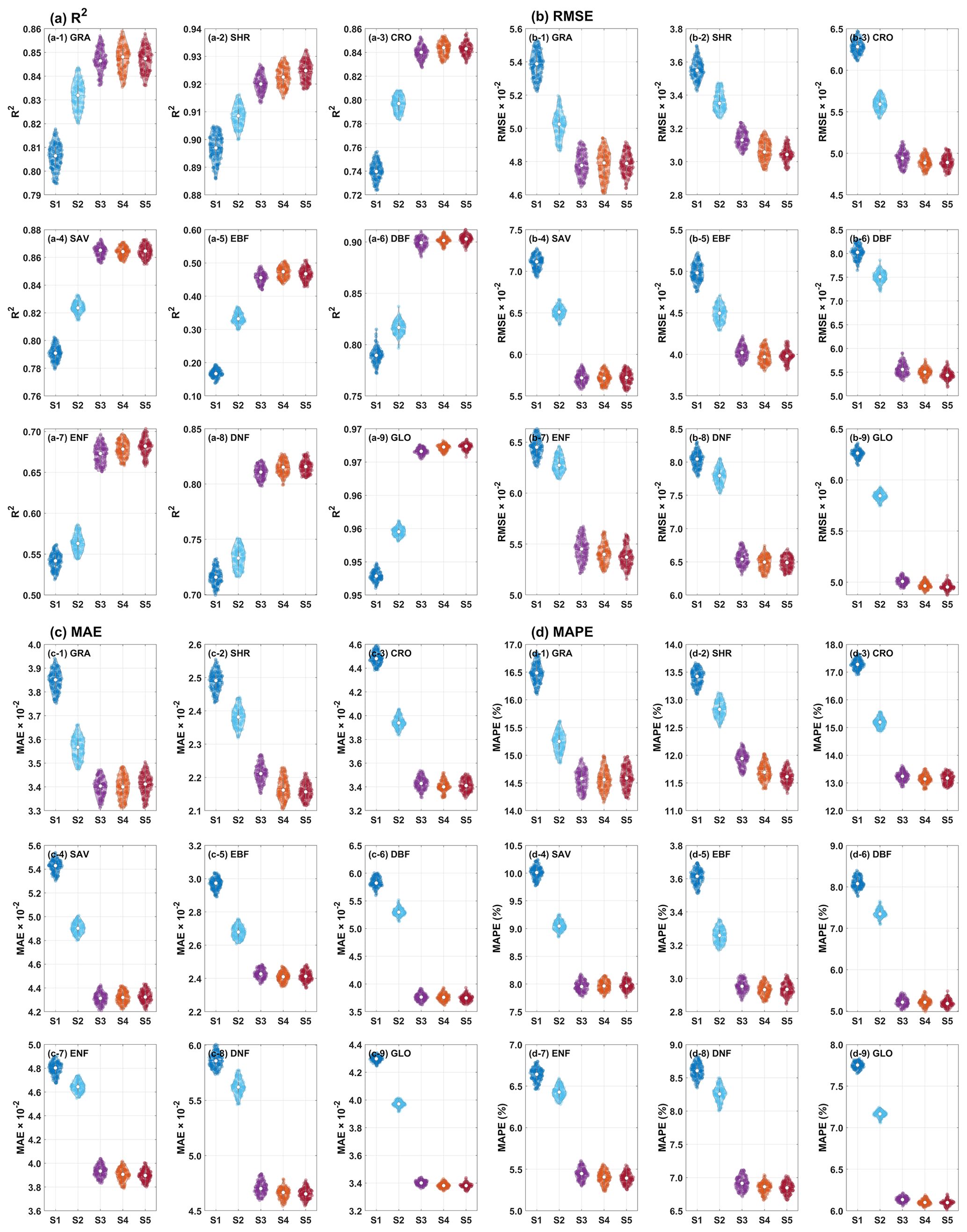
Figure 4 Performance of different combinations of explanatory variables (S1 to S5) for BPNN models. Panels (a), (b), (c), and (d) show the R², RMSE, MAE, and MAPE of the BPNN models, respectively. GLO represents the global vegetation biome. The combinations of explanatory variables are (S1) NDVI alone; (S2) NDVI and spatial information (longitude and latitude); (S3) NDVI, spatial information, and time information (month); (S4) NDVI, spatial information, time information, and NOAA satellite number; and (S5) NDVI, spatial information, time information, NOAA satellite number, and years since its launch.

4.2.2 Selection of explanatory variables for the BPNN model

The accuracy of BPNN models under different combinations of explanatory variables (S1 to S5) is shown in Fig. 4. The addition of spatial location significantly improved the accuracy of predicted NDVI for the vegetation biome types that are distributed worldwide. The improvement has not been observed for vegetation biome types that are relatively concentrated (e.g., ENF and DNF). The addition of temporal information improved the accuracy of vegetation types with prominent seasonal variations such as DBF and DNF. Finally, adding the NOAA satellite number and orbit time could also improve the accuracy of BPNN models, especially for SHR.

For the combination containing all explanatory variables (S5), the R² of most vegetation biome types except for EBF and ENF was >0.8. For vegetation biomes overall, the R² reached 0.96, and the relative error was only 11.35 %. Therefore, all available explanatory variables, i.e., the NDVI, longitude, latitude, month, NOAA satellite number, and years since the NOAA satellite's launch, contributed to the BPNN model in this study.

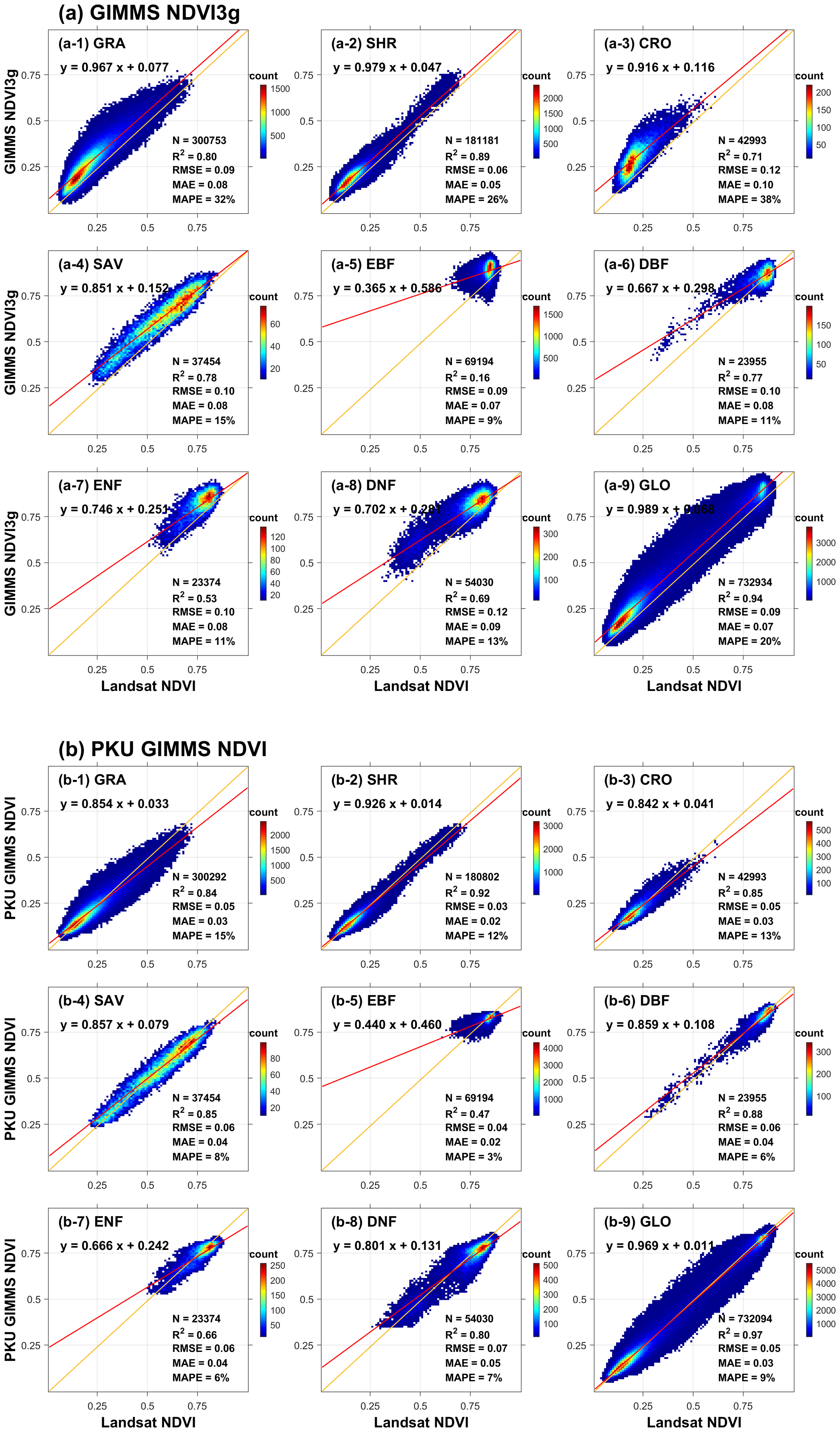
Figure 5 Direct validation of the (a) GIMMS NDVI3g and (b) PKU GIMMS NDVI (before consolidation) products. Individual Landsat NDVI samples from 1984 to 2015 were used in the validation at a $\mathrm{1}/\mathrm{12}$^∘ resolution. Orange lines represent a 1:1 line. GLO represents the global vegetation biome.

4.2.3 Direct validation of PKU GIMMS NDVI and GIMMS NDVI3g

Our PKU GIMMS NDVI product (before consolidation) and the GIMMS NDVI3g product were directly verified with the remaining 20 % of the Landsat NDVI samples from 1984 to 2015 (Fig. 5). Overall, the accuracy of the PKU GIMMS NDVI (R²=0.97, RMSE = 0.05, MAE = 0.03, MAPE = 9 %) was higher than that of the GIMMS NDVI3g (R²=0.94, RMSE = 0.09, MAE = 0.07, MAPE = 20 %) in all metrics. Among different vegetation biome types, the NDVI quality of SHR (GIMMS NDVI3g: R²=0.89, RMSE = 0.06, MAE = 0.05, MAPE = 26 % and PKU GIMMS NDVI: R²=0.92, RMSE = 0.03, MAE = 0.02, MAPE = 12 %) was higher than that of other biome types. The accuracy of EBF was relatively low for both products (GIMMS NDVI3g: R²=0.16, RMSE = 0.09, MAE = 0.07, MAPE = 9 % and PKU GIMMS NDVI: R²=0.47, RMSE = 0.04, MAE = 0.02, MAPE = 3 %). The reason was that EBF is primarily distributed in tropical areas where the quality of remote sensing data is poor due to frequent clouds and rains.

For the GIMMS NDVI3g product, the accuracy differences between vegetation biome types were evident (Fig. 5). The NDVI of SHR (RMSE = 0.06, MAE = 0.05), SAV (RMSE = 0.10, MAE = 0.08), ENF (RMSE = 0.10, MAE = 0.08), and DNF (RMSE = 0.12, MAE = 0.09) has been systematically overestimated (Fig. 5a). GRA and CRO were also overestimated, mainly when NDVI values were high (Fig. 5a). The NDVI of EBF has a rather low accuracy in the GIMMS NDVI3g products, with an R² of only 0.16. For the PKU GIMMS NDVI product, its performance in different vegetation biome types was more stable (R²: 0.47 to 0.92; RMSE: 0.03 to 0.07; MAE: 0.02 to 0.05; MAPE: 3 % to 15 %), and the scatter points remained near the 1:1 line (Fig. 5). In particular, the R² of EBF was improved to 0.47 in the PKU GIMMS NDVI.

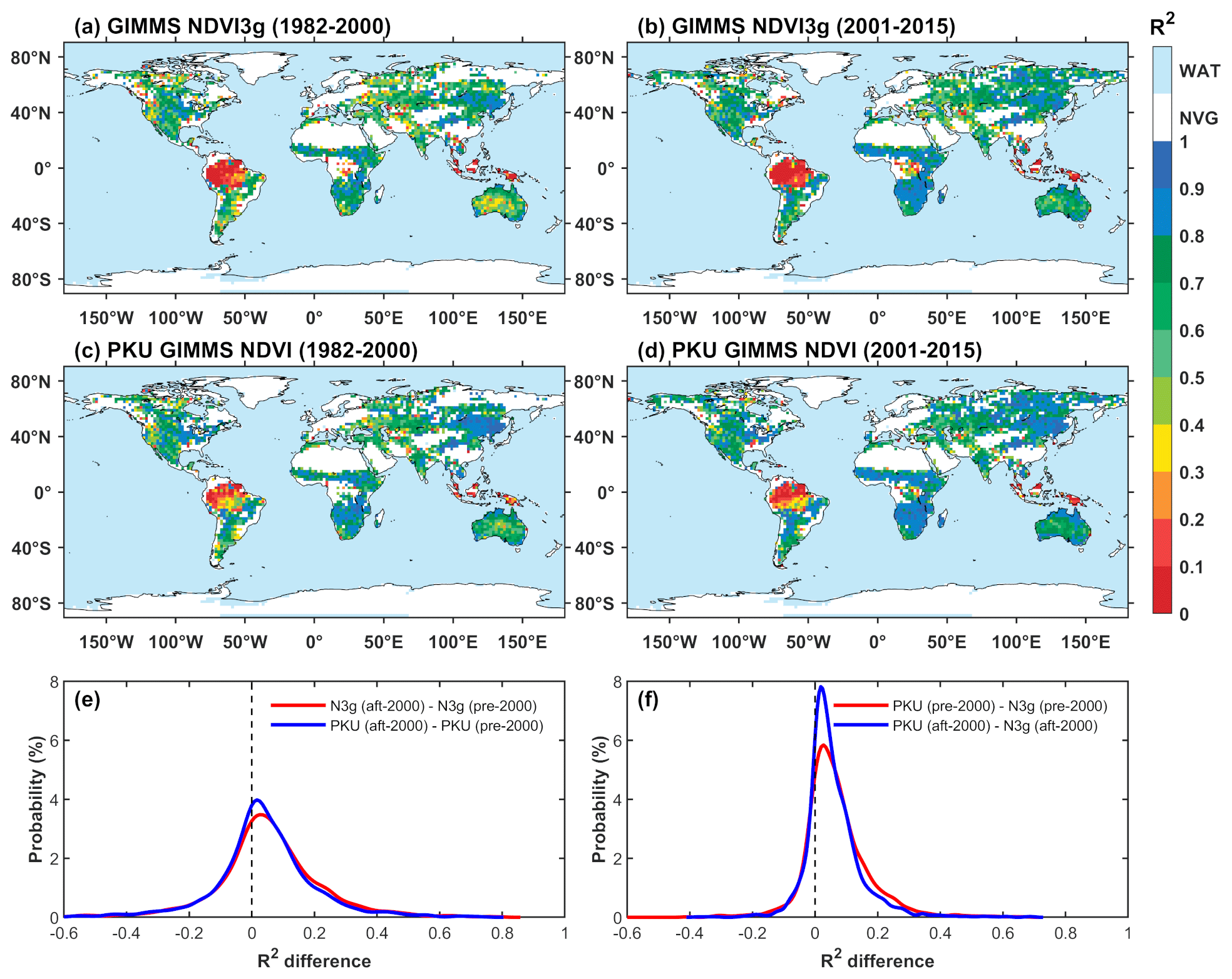
Figure 6 Accuracies of the GIMMS NDVI3g and PKU GIMMS NDVI (before consolidation) products measured by R² for pre-MODIS (1982–2000) and MODIS (2001–2015) period. The R² was calculated between the NDVI products and Landsat NDVI samples. Panels (a) to (d) show the spatial distributions of R² in 2^∘ × 2^∘ grids. Non-vegetated grids and grids with less than 20 validation samples are marked in white. Panels (e) and (f) show the probability distribution of R² differences between the two periods (before 2000 and after 2000) and between the two products (GIMMS NDVI3g and PKU GIMMS NDVI), respectively.

4.2.4 Accuracy of PKU GIMMS NDVI and GIMMS NDVI3g in space

The accuracies of the PKU GIMMS NDVI (before consolidation) and GIMMS NDVI3g products exhibited strong spatial heterogeneity (Fig. 6). The low-accuracy areas were primarily concentrated in the tropics and high northern latitudes, and the high-accuracy regions were concentrated in the mid-latitudes of the Eurasian continent, the Great Plains of the United States, and savanna-dominated areas of Africa and Australia. In the tropical rainforest area where both products had relatively low accuracies, the PKU GIMMS NDVI performed better, especially in Southeast Asia and the northwestern Amazon region. However, the improvement of PKU GIMMS NDVI over GIMMS NDVI3g was not significant along the western coast of the European continent and southeast China, probably due to the small number of training samples.

Probability density diagrams were drawn to show NDVI differences between two periods (before and after 2000) (Fig. 6e) and between two products (Fig. 6f). The accuracy of both NDVI products after 2000 was generally higher than before 2000. The difference was more evident for the GIMMS NDVI3g product (Fig. 6e). The PKU GIMMS NDVI improved the accuracies over the GIMMS NDVI3g, especially for the period before 2000 (Fig. 6f).

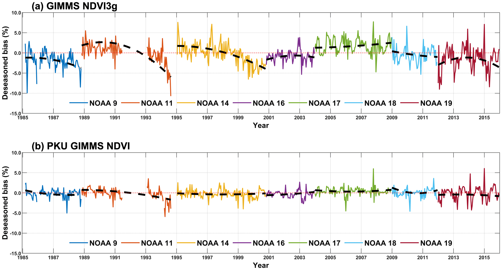
Figure 7 Temporal variations of NDVI bias percentage in EBF for (a) the GIMMS NDVI3g product and (b) the PKU GIMMS NDVI (before consolidation) product. The dashed black line represents the interannual trend extracted by the EEMD method. Values from different NOAA satellite missions are distinguished with colors.

4.2.5 Alleviation of the orbital drift and sensor degradation effect

As shown in Fig. 7, the GIMMS NDVI3g product exhibited evident false signals in the EBF region, which agreed with the previous findings (Tian et al., 2015). The NDVI bias from different NOAA satellites significantly varied, which may cause the jump phenomenon between NOAA missions. Before 2000, the effects of orbital drift and sensor degradation were evident at the last phases of satellite launch. This is especially true for the NOAA 11 satellite (Fig. 7a). The effect became relatively small for NOAA satellites launched after 2000. In the PKU GIMMS NDVI (before consolidation) product, the impact from orbital drift and sensor degradation has been effectively rectified (Fig. 7b). NDVI bias did not change significantly over time, indicating that the PKU GIMMS NDVI product had good temporal consistency.

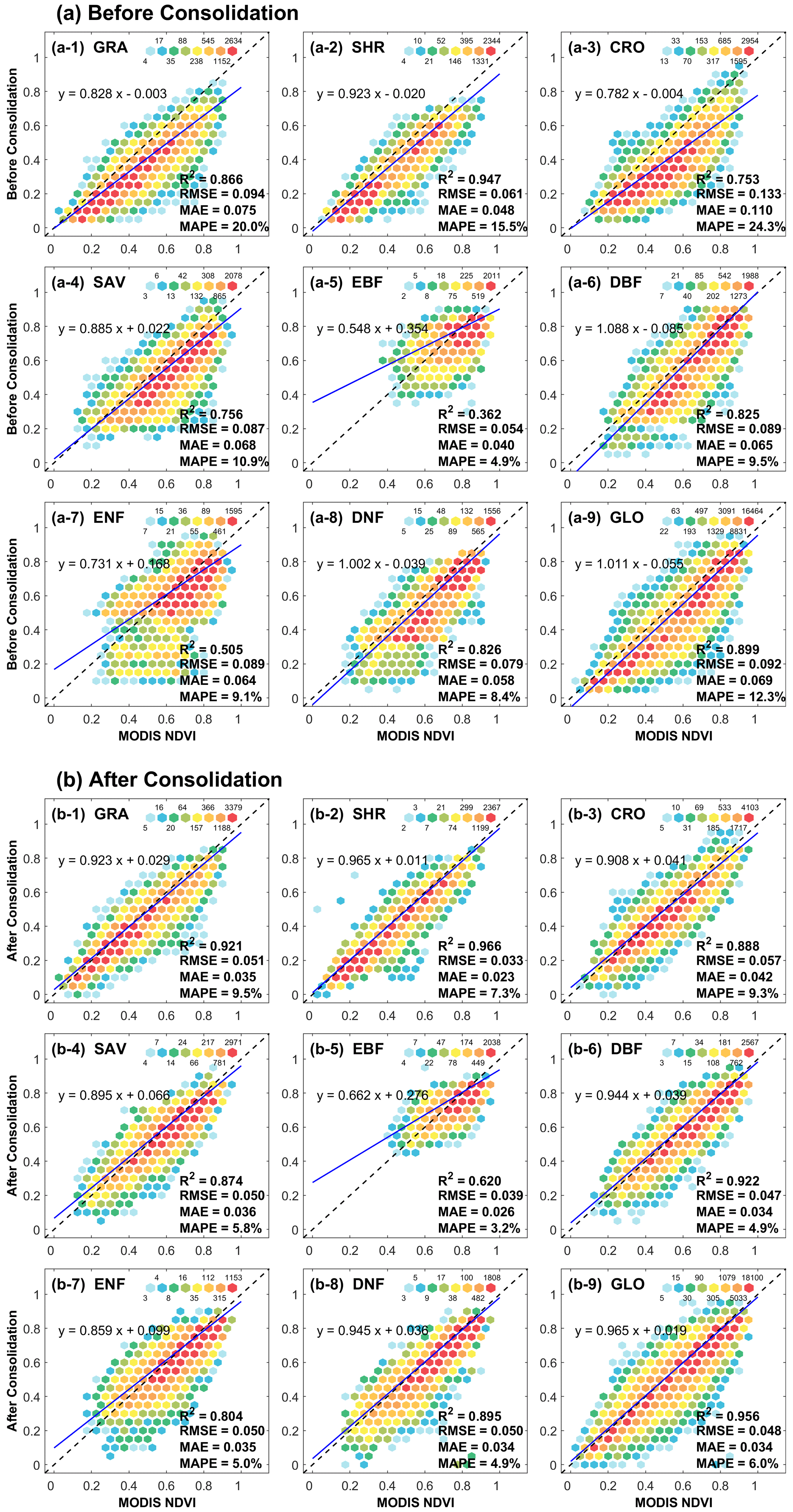
Figure 8 Validation of the PKU GIMMS NDVI product (a) before and (b) after consolidation. The validation was performed using 1000 MODIS NDVI samples at a $\mathrm{1}/\mathrm{12}$^∘ resolution for each vegetation biome type from 2003 to 2015.

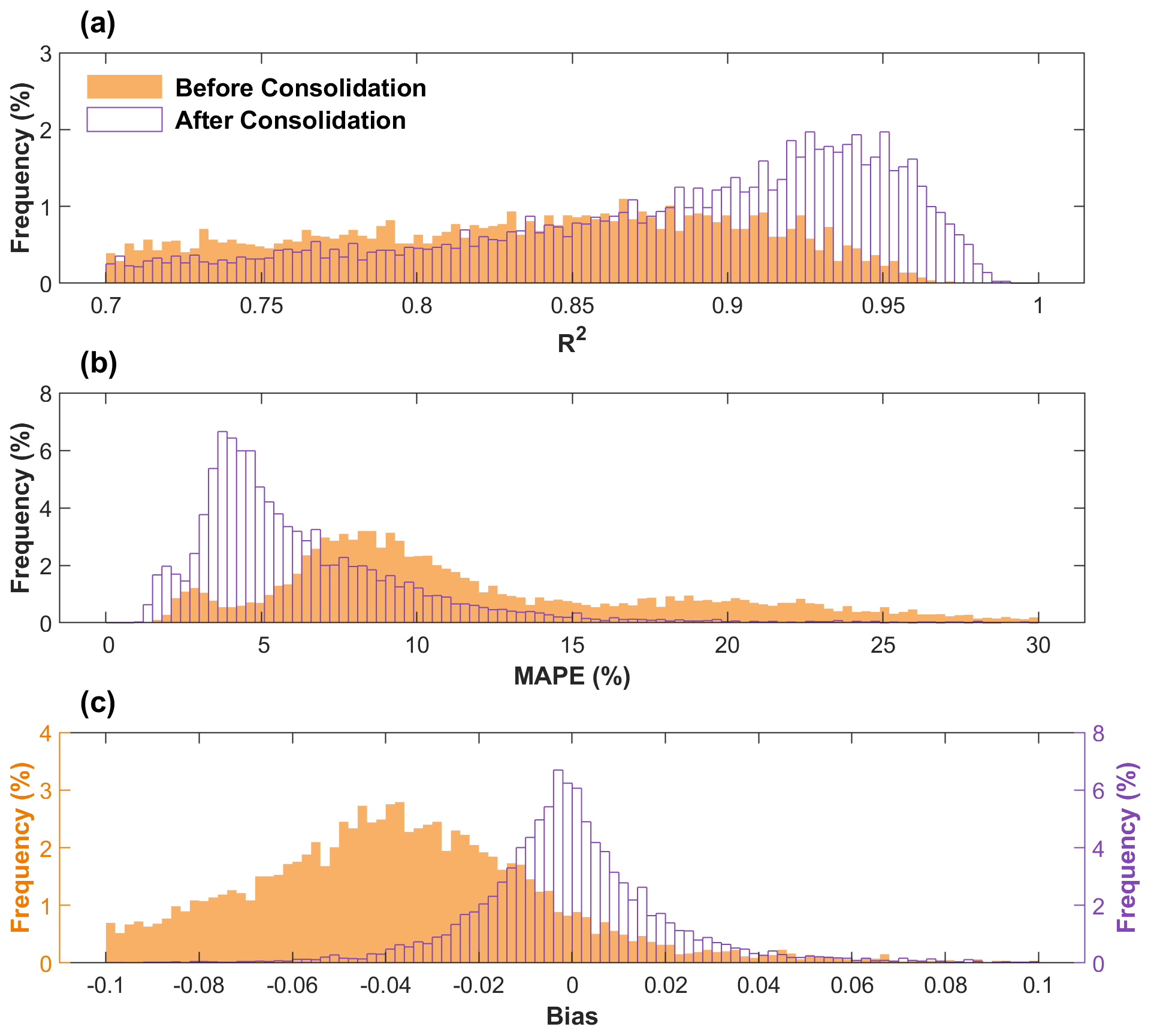
Figure 9 Distribution of the accuracy metrics before and after consolidation. The accuracy metrics include (a) R², (b) MAPE, and (c) bias. The distribution was calculated using 8000 random sample points from 2003 to 2015 with MODIS NDVI as the true value.

4.3 Consolidated PKU GIMMS NDVI

4.3.1 Comparison with MODIS NDVI

The consolidation process improved the consistency level between PKU GIMMS NDVI and MODIS NDVI from acceptable (R²=0.899, RMSE = 0.092, MAE = 0.069, and MAPE = 12.3 %) (Fig. 8a–9) to high (R²=0.956, RMSE = 0.048, MAE = 0.034, and MAPE = 6.0 %) (Fig. 8b–9). Specifically, the PKU GIMMS NDVI before data consolidation was systematically lower than MODIS NDVI, but the relationship approached 1:1 after consolidation. The improvement in consistency was different among vegetation biome types. CRO and GRA had the greatest improvement, as their MAPE decreased from 24.3 % and 20.0 % to 9.3 % and 9.5 %, respectively (Fig. 8a and b). The probability distribution densities of R², MAPE, and bias were also analyzed based on NDVI values before and after consolidation at all samples (8000) (Fig. 9). The results show that the R² was improved (Fig. 9a), and the MAPE was significantly decreased (Fig. 9b) after consolidation.

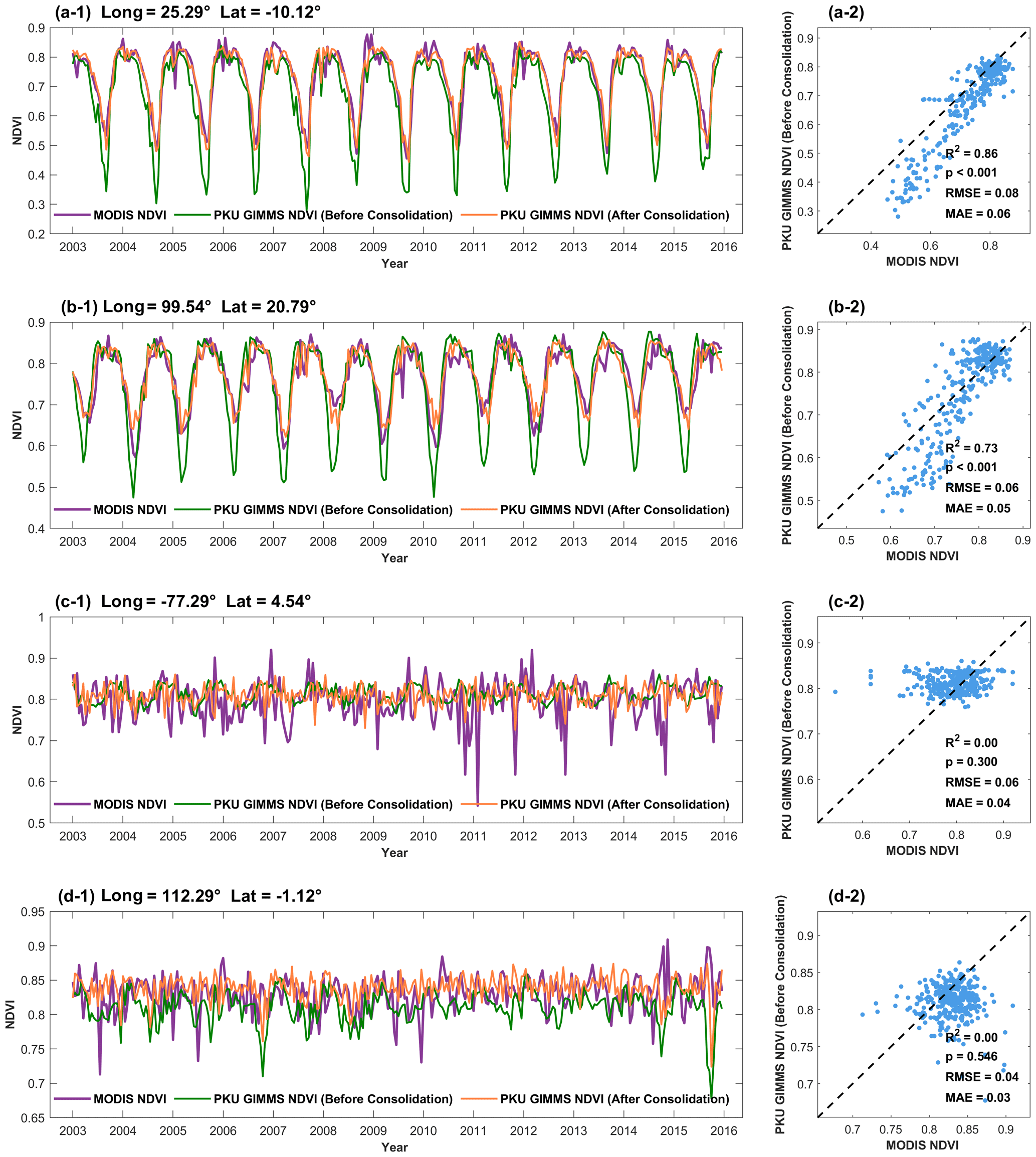
Figure 10 Selected EBF locations illustrating the consistency between the PKU GIMMS NDVI product (before and after consolidation) and the MODIS NDVI product. Panels (a) and (b) show the locations with significant pixel-wised RF regression models. Panels (c) and (d) show the locations with insignificant models. NDVI values outside 2 standard deviations were treated as outliers and removed.

For EBF, the improvement in consistency after consolidation was relatively small (MAPE: 4.9 % to 3.2 %). The pixel-wised RF regression model for data consolidation was significant for selected EBF locations (Fig. 10a and b), but it was not for other locations. Due to frequent clouds and rains, both PKU GIMMS NDVI and MODIS NDVI could present maximum noises (Fig. 10c and d). In this case, it was determined that individual MODIS NDVI values were no longer reliable as a benchmark in the regression model, and a simple mean-value aligning method was adopted.

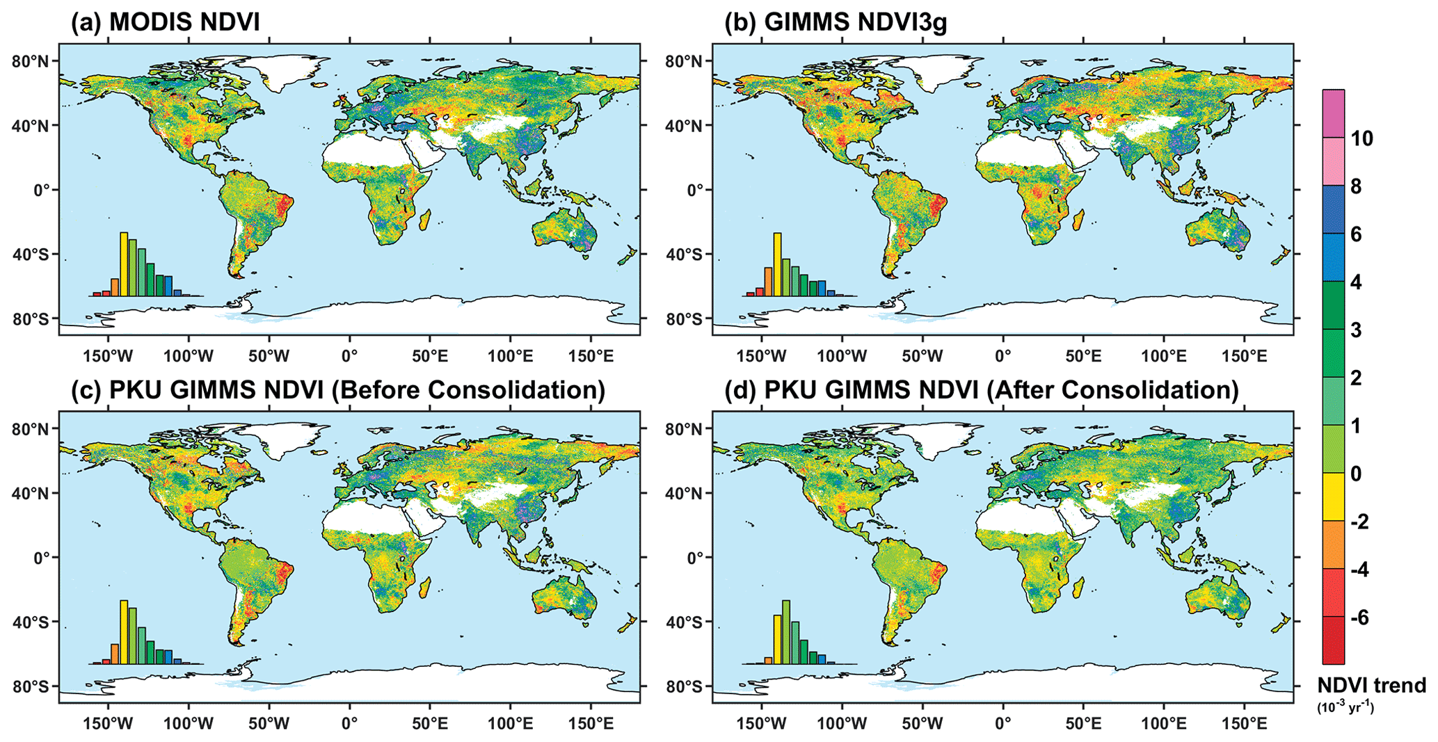
Figure 11 Distribution of the NDVI trend from 2003 to 2015. The NDVI trend is calculated based on the time series of annual average NDVI from (a) MODIS NDVI, (b) GIMMS NDVI3g, (c) PKU GIMMS NDVI (before consolidation), and (d) PKU GIMMS NDVI (after consolidation). The non-vegetation area is marked in white.

4.3.2 Vegetation trend analysis

Figure 11 shows the distribution of slopes in the linear regression for the GIMMS NDVI3g, MODIS NDVI, and PKU GIMMS NDVI (before and after consolidation) products at $\mathrm{1}/\mathrm{12}$^∘ grids. Overall, these products showed similar spatial patterns in some global hot spots. For example, all of them capture the greening trend in China and India. However, the GIMMS NDVI3g products showed the opposite trend against MODIS NDVI and PKU GIMMS NDVI products in the tropical evergreen broadleaf forest regions of Africa and Southeast Asia (Fig. 11).

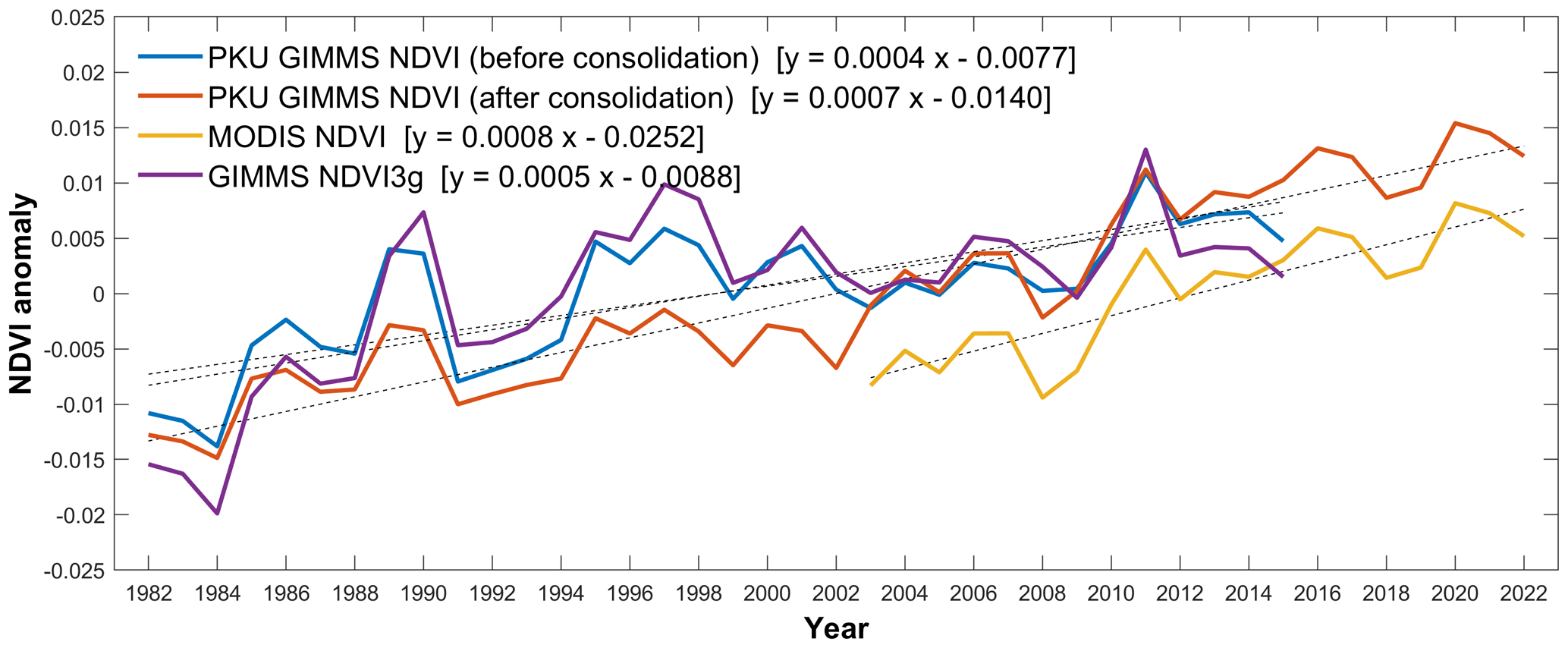
Figure 12 Annual anomalies and trends of PKU GIMMS NDVI (before consolidation), PKU GIMMS NDVI (after consolidation), MODIS NDVI, and GIMMS NDVI3g. The NDVI anomalies were calculated as area-weighted annual averages.

The time series of annual NDVI anomalies and trends from different products are shown in Fig. 12. All products presented a similar shape of anomalies in their overlapping periods. During 1982–2015, PKU GIMMS NDVI before consolidation had a similar trend with GIMMS NDVI3g ($\mathrm{0.4}\times {\mathrm{10}}^{-\mathrm{3}}$ vs. $\mathrm{0.5}\times {\mathrm{10}}^{-\mathrm{3}}$ yr⁻¹). During 2003–2015 when all NDVI products were available, PKU GIMMS NDVI after consolidation ($\mathrm{0.9}\times {\mathrm{10}}^{-\mathrm{3}}$ yr⁻¹) and MODIS NDVI ($\mathrm{0.9}\times {\mathrm{10}}^{-\mathrm{3}}$ yr⁻¹) had the same vegetation trend (trend values not shown in the figure), slightly higher than PKU GIMMS NDVI before consolidation ($\mathrm{0.7}\times {\mathrm{10}}^{-\mathrm{3}}$ yr⁻¹), followed by GIMMS NDVI3g ($\mathrm{0.5}\times {\mathrm{10}}^{-\mathrm{3}}$ yr⁻¹). In the EBF area, GIMMS NDVI3g showed a browning trend since 2003 due to the impact of orbital drift and sensor degradation (Fig. A1), which was consistent with the research by Wang et al. (2022). In PKU GIMMS NDVI products, the effect of orbital drift and sensor degradation has been alleviated. It showed a greening trend in EBF, consistent with MODIS NDVI (Fig. A1).

5 Data availability

The spatiotemporally consistent global dataset of the GIMMS Normalized Difference Vegetation Index (PKU GIMMS NDVI) generated in this study is openly available at https://doi.org/10.5281/zenodo.8253971 (Li et al., 2023). It covers the whole global vegetation area at half-month temporal resolution and $\mathrm{1}/\mathrm{12}$^∘ spatial resolution from 1982 to 2022. It is available in geographic lat–long projection and TIFF format. In the same repository, we have also provided the version of PKU GIMMS NDVI before consolidation with MODIS NDVI (1982–2015). We strongly recommend users read the Readme file in the repository and properly handle the fill value and the quality control flag in the dataset.

6 Discussion and conclusion

6.1 Improvements over other long-term global NDVI products

The generation of long-term global NDVI products has been challenging due to the uncertainties associated with the impacts of satellite orbital drift and sensor degradation/calibration; artifacts related to data processing and analysis; and effects from the atmosphere, BRDF, scale, and topography, etc. (Zeng et al., 2022). While a lot of work remains to be done, the current NDVI products have made substantial progress in dealing with selected uncertainties and improving the data quality. Depending on the type of uncertainty, many methods and data have been introduced with different degrees of succession. For example, the GIMMS NDVI3g product has primarily focused on identifying the systematic deviations between AVHRR-2 and AVHRR-3, caused by differences in the sensor characteristics, and on resolving the inconsistency between AVHRR NDVI products (Pinzon and Tucker, 2014).

The significance of the PKU GIMMS NDVI product was the use of massive representative high-quality Landsat NDVI samples across the globe from 1984 to 2015. More than 12 million samples of different vegetation biome types were extracted to create temporally consistent Landsat data (Fig. 2), and approximately 3.6 million Landsat NDVI samples were obtained to generate PKU GIMMS NDVI. The number, temporal coverage, and spatial coverage of the samples (Fig. 3) have been unparalleled compared to preceding long-term NDVI products that also employed samples from other sensors, most of which became available only after the late 1990s (e.g., SeaWiFS: 1997–2010; SPOT-VGT: 1999–2014; MODIS: since 2001; VIIRS: since 2012). The massive Landsat NDVI samples paved the way for accurate Landsat sensor cross-calibration (Fig. 2) and PKU GIMMS NDVI generation (Figs. 5 and 6). They helped efficiently remove the uncertainties from NOAA orbital drift and AVHRR sensor degradation (Fig. 7). While this is out of the scope of the current study, future evaluation work is suggested to comprehensively compare the PKU GIMMS NDVI to other global long-term NDVI products such as the LTDR4 and VIP3.

The improvements in PKU GIMMS NDVI may help to clarify some discrepancies between existing NDVI products, for instance, the vegetation trend in humid tropical regions after 2000. In these regions, current findings from multiple studies suggested that GIMMS-based NDVI presented a decreasing trend, while MODIS-based NDVI presented an increasing trend (Fensholt and Proud, 2012; Tian et al., 2015; Wang et al., 2022). Possible reasons could be the uncertainties from NDVI saturation or lack of high-quality data (Fensholt and Proud, 2012; Wang et al., 2022) and orbital drift effects for GIMMS NDVI (Tian et al., 2015). In the generation of PKU GIMMS NDVI, these uncertainties have been well accounted for, and we found an increasing NDVI trend in tropical regions after 2000, both before and after data consolidation with MODIS NDVI.

6.2 Uncertainty source

Despite our efforts to improve the number and quality of the Landsat NDVI samples, uncertainties remain. Besides those related to the Landsat NDVI itself (such as the geometric and radiometric errors), one major source of uncertainty is the sample size. For certain vegetation biomes, the number of samples in some regions (such as EBF and northern high latitudes) may be insufficient due to the constraints in solar zenith angle and environmental conditions. Our results indicated that the accuracy of BPNN models was lower (despite being acceptable) in the regions with fewer samples (Figs. 3 and 6). Future research in these regions should include samples from other satellite data as supplements.

Another source of uncertainty is the BNPP model. We developed individual BPNN models for vegetation biome types. As such, errors in the static vegetation biome map and in the MODIS land cover product and the heterogeneity of Earth's surface might all diminish the model performance. As input in the BNPP model, GIMMS NDVI3g could also transmit its uncertainties to the PKU GIMMS NDVI. Furthermore, subsequent research can include other explanatory variables in the BPNN, such as the environmental variables (e.g., solar radiation, temperature, and precipitation), to better explain NDVI variations.

6.3 A summary of the PKU GIMMS NDVI product

In this study, a new version of GIMMS NDVI product, i.e., the PKU GIMMS NDVI, was developed using the BPNN model, employing a large number of global high-quality Landsat NDVI samples and a data consolidation method that employed MODIS NDVI. The PKU GIMMS NDVI covers a time span of 1982 to 2022, with a spatial resolution of $\mathrm{1}/\mathrm{12}$^∘ and a temporal resolution of half-month. The high reliability and high accuracy of the PKU GIMMS NDVI product is demonstrated by the following:

• The Landsat NDVI samples used to generate the PKU GIMMS NDVI were abundant (3.6 million), well distributed, representative, and high-quality. The inter-comparison between NDVI of different Landsat sensors after calibration showed high R² (>0.98), low RMSE (<0.04), low MAE (<0.02), and low MAPE (<6 %).

• Assessing against the Landsat NDVI, the PKU GIMMS NDVI had high overall accuracies (R²=0.97, RMSE = 0.05, MAE = 0.03, MAPE = 9 %) and high accuracies for individual vegetation biomes (R²: 0.47 to 0.92; RMSE: 0.03 to 0.07; MAE: 0.02 to 0.05; MAPE: 3 % to 15 %). It performed better than the GIMMS NDVI3g (overall: R²=0.94, RMSE = 0.09, MAE = 0.07, MAPE = 20 %), especially for the tropical evergreen broadleaf forests (EBF) (R²=0.16 in the GIMMS NDVI3g; R²=0.47 in the PKU GIMMS NDVI).

• The PKU GIMMS NDVI efficiently removed the effects of NOAA orbital drift and AVHRR sensor degradation.

• During the overlapping period, the consolidated PKU GIMMS NDVI has a good agreement with MODIS NDVI in values (R² = 0.956, RMSE = 0.048, MAE = 0.034, and MAPE = 6.0 %) and in the vegetation trend ($\mathrm{0.9}\times {\mathrm{10}}^{-\mathrm{3}}$ yr⁻¹).

The long-term, continuous, and reliable PKU GIMMS NDVI for the past 40 years can provide more accurate vegetation monitoring in the context of climate change. The framework proposed in this study which used high-quality Landsat samples with BPNN and other explanatory variables (the longitude and latitude, associated month, and the NOAA number and years since launch) can also benefit the development of other remote sensing products of land surface parameters (e.g., the development of LAI products).

Appendix A

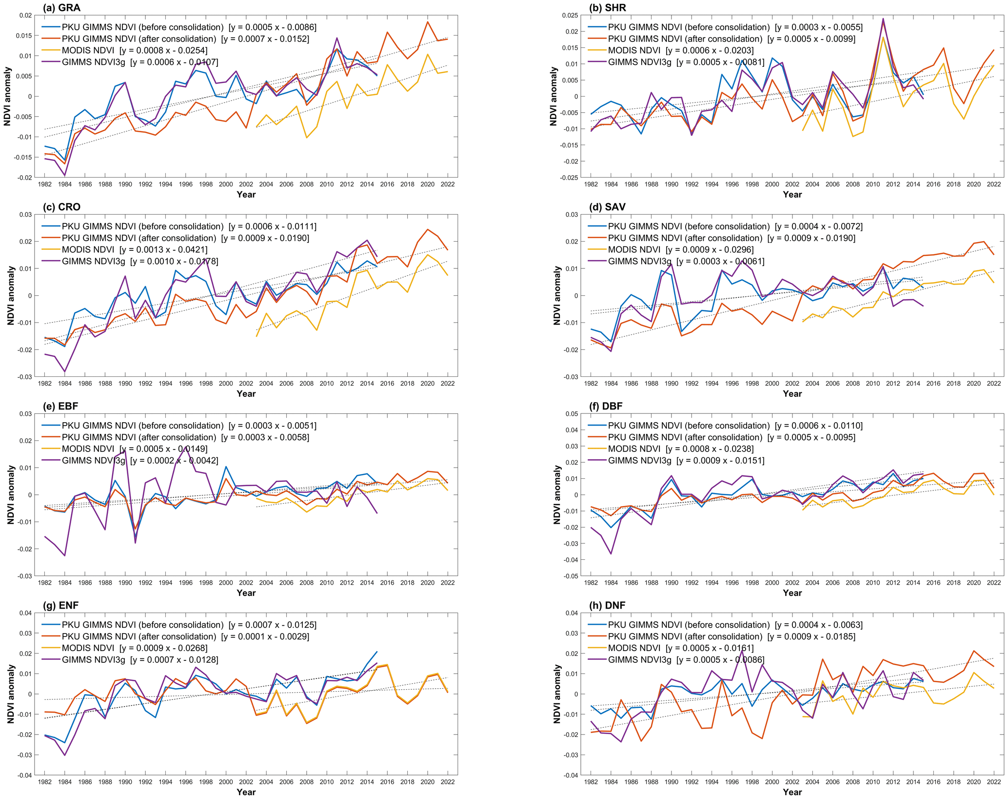
Figure A1 Annual anomalies and trends of PKU GIMMS NDVI (before consolidation), PKU GIMMS NDVI (after consolidation), MODIS NDVI, and GIMMS NDVI3g for different vegetation biome types. The NDVI anomalies were calculated as area-weighted annual averages.