A first global height-resolved cloud condensation nuclei data set derived from spaceborne lidar measurements

We present a global multiyear height-resolved data set of aerosol-type-specific cloud condensation nuclei concentrations (n_CCN) estimated from the spaceborne lidar aboard the Cloud-Aerosol Lidar and Infrared Pathfinder Satellite Observation (CALIPSO) satellite. For estimating n_CCN, we apply the recently introduced Optical Modelling of the CALIPSO Aerosol Microphysics (OMCAM) algorithm to the CALIPSO Level 2 Aerosol Profile product. The estimated n_CCN are then gridded into a uniform latitude–longitude grid of $\mathrm{2}{}^{\circ }\times \mathrm{5}{}^{\circ }$, a vertical grid of resolution 60 m from the surface to an altitude of 8 km, and a temporal resolution of 1 month. The data span a total of 186 months, from June 2006 to December 2021. In addition, we provide a 3D aerosol-type-specific climatology of n_CCN produced using the complete time series. We further highlight some potential applications of the data set in the context of aerosol–cloud interactions. The complete data set can be accessed at https://doi.org/10.1594/PANGAEA.956215 (Choudhury and Tesche, 2023).

1 Introduction

Airborne aerosols can serve as cloud condensation nuclei (CCN) to form liquid cloud droplets and influence the properties of clouds. For instance, an increase in the number of aerosols that can act as CCN may result in more but smaller cloud droplets at a constant cloud liquid water content. As a result, the effective surface area of the cloud available to interact with incoming solar radiation increases, enhancing the cloud albedo and cooling the Earth (Twomey, 1974). Furthermore, it may take longer for these smaller droplets to grow large enough to form precipitation, leading to an increase in cloud lifetime and cloud cover and, thus, imposing an additional cooling effect (Albrecht, 1989). Understanding and quantifying such aerosol–cloud interactions (ACIs) is necessary to predict and mitigate their potential impacts on the Earth's radiation budget (Forster et al., 2021).

Only a fraction of aerosols, depending primarily on their size and, to a lesser extent, chemical composition, can act as CCN (Dusek et al., 2006). This dependency is further regulated by atmospheric water vapour supersaturation, which is a function of meteorological parameters like updraught velocity, humidity, temperature, and pressure (Seinfeld et al., 2016). The supersaturation near the cloud base of boundary layer clouds is usually about 0.15 %–0.20 %. Under such conditions, continental and marine aerosols with a dry radius greater than 50 nm (n_50,dry) and dust aerosols with a dry radius greater than 100 nm (n_100,dry) form the reservoir of most favourable CCN (Mamouri and Ansmann, 2016; Choudhury and Tesche, 2022b). The concentration of such particles varies with geographical location and, as per the findings from surface in situ measurements, can range from about 10 cm⁻³ under pristine conditions to as much as 10⁵ cm⁻³ in polluted urban air masses (Schmale et al., 2018). Similar orders of magnitude of variation in CCN concentrations are also seen in the vertical dimension, with the highest concentrations close to the surface and only a few particles in the upper troposphere (Brock et al., 2021; Zhang et al., 2022). Given the wide range of CCN concentrations, global information on the horizontal and vertical distribution of CCN is necessary to accurately quantify the impact of ACIs on climate (Bellouin et al., 2020; Quaas et al., 2020).

Today, there is a lack of observation-based global CCN data. While climate model outputs can be used to study the global distribution of CCN, they have been identified to underestimate CCN at the surface by a normalized mean error of about 40 % to 80 % depending on the geographical location (Fanourgakis et al., 2019a). In situ measurements, despite being performed continuously with a high temporal resolution, are localized to specific land sites and do not cover oceans. Also, such measurements are usually limited to the surface, as it is not feasible to operate airborne measurements over longer periods. Here, satellite remote sensing, specifically based on spaceborne lidar, emerges as the best way to obtain a height-resolved, long-term, and observation-based global picture of atmospheric CCN concentrations.

The polar-orbiting Cloud-Aerosol Lidar and Infrared Pathfinder Satellite Observation (CALIPSO) satellite includes the Cloud-Aerosol Lidar with Orthogonal Polarization (CALIOP) instrument, which provides height-resolved information on aerosol optical properties for different aerosol types (Winker et al., 2009). Choudhury and Tesche (2022a) present an algorithm that uses the spaceborne lidar measurements and the aerosol microphysics included in the CALIPSO aerosol model (Omar et al., 2009) to estimate height-resolved cloud-relevant aerosol number concentrations (n_50,dry and n_100,dry) and CCN concentrations. The results are found to be consistent with in situ measurements at various geographic locations over land and ocean covering different aerosol environments (Choudhury et al., 2022; Choudhury and Tesche, 2022b; Aravindhavel et al., 2023). This highlights the potential of CALIOP measurements with respect to producing an unprecedented global CCN data set from satellite observations.

In this paper, we present a global monthly 3D data set of the number concentration of CCN (n_CCN) for different aerosol types that has been constructed by applying the CCN retrieval algorithm of Choudhury and Tesche (2022a) to more than 15 years (June 2006 to December 2021) of CALIPSO Level 2 Aerosol Profile data. We also provide seasonal and annual climatologies of n_CCN estimated from the monthly data. All data sets are produced at a uniform latitude–longitude grid of $\mathrm{2}{}^{\circ }\times \mathrm{5}{}^{\circ }$ resolution and a vertical resolution of 60 m, consistent with the grid of the CALIPSO Level 3 monthly product (Tackett et al., 2018). The data records are given in Network Common Data Form (NetCDF) format separately for each year and can be accessed at https://doi.org/10.1594/PANGAEA.956215 (Choudhury and Tesche, 2023). Details regarding the input data and algorithm used to produce the CCN data set are discussed in Sect. 2. Section 3 provides the description of the pre- and post-processing steps involved in the production of the gridded data and elaborates on the physical meaning and application of all of the variables stored in the data. The estimated seasonal and annual n_CCN climatologies and a comparison of the annual averaged n_CCN with the global climate model outputs from Fanourgakis et al. (2019a) for the year 2011 are presented in Sect. 4. We conclude the paper with potential applications of the global CCN data set in Sect. 6.

2 Data and CCN retrieval

2.1 CALIPSO aerosol profile product

The CALIPSO polar-orbiting satellite has been operational since June 2006. CALIOP, a nadir-viewing elastic-backscatter lidar, is the principal payload on CALIPSO. It measures vertical profiles of aerosol and cloud properties at two wavelengths: 532 and 1064 nm. In this work, we use aerosol optical properties at 532 nm from the CALIPSO Level 2 version 4.20 (4.21 since July 2020) aerosol profile product (NASA/LARC/SD/ASDC, 2018), such as the aerosol extinction coefficient (α), backscatter coefficient (β), and depolarization ratio (δ). All parameters are provided at an along-track horizontal resolution of 5 km with a vertical resolution of 60 m for tropospheric aerosols. We further use the atmospheric volume description flag to access the information on aerosol type, which contains seven categories: marine, desert dust, polluted continental, clean continental, elevated smoke, polluted dust, and dusty marine. These aerosol types are classified based on the type of underlying surface; the aerosol optical properties, such as the column-integrated attenuated backscatter coefficient and the initial estimated particle depolarization ratio at 532 nm; and the height of the retrieval (Kim et al., 2018). Additionally, quality control flags are utilized to screen the data for the most reliable retrievals (further details given in Sect. 3). We also use the auxiliary profiles of ambient relative humidity (RH) and pressure in the Level 2 data product. These are derived from the Global Modelling and Assimilation Office (GMAO) Global Data Assimilation System (GDAS; Molod et al., 2015). The Level 2 Aerosol Profile data considered in this study cover a total of 186 months in the time period from June 2006 to December 2021 (data for February 2016 are not available). Note that CALIPSO underwent an orbit adjustment in September 2018 to synchronize its path with that of the CloudSat satellite. Although this orbital shift resulted in a slight variation in the geographic region observed by CALIPSO, there are currently no known issues associated with CALIPSO’s retrieval quality as a result of this transition.

2.2 Model data

We use the modelled n_CCN from Fanourgakis et al. (2019a) for comparison to CALIPSO estimates. The data are comprised of annual average surface n_CCN at different supersaturations for the year 2011 with a latitude–longitude resolution of $\mathrm{1}{}^{\circ }\times \mathrm{1}{}^{\circ }$ and were obtained from the output of 15 global models. Details on the model configurations and aerosol emission inventories used for modelling n_CCN are described comprehensively in Fanourgakis et al. (2019a). The data can be downloaded from https://doi.org/10.5281/zenodo.3265866 (Fanourgakis et al., 2019b).

2.3 CCN retrieval algorithm

The CCN retrieval algorithm used in this work is based on the Optical Modelling of the CALIPSO Aerosol Microphysics (OMCAM) algorithm. The algorithm is described comprehensively in Choudhury and Tesche (2022a) and Choudhury et al. (2022). In this section, we briefly review the main steps involved in OMCAM.

The OMCAM algorithm first estimates the aerosol size distribution by using (i) CALIPSO-derived aerosol-type-specific extinction coefficients, (ii) their corresponding microphysical properties (normalized volume size distributions and refractive indices), and (iii) an optical modelling package called Modelled Optical Properties of enseMbles of Aerosol Particles (MOPSMAP; Gasteiger and Wiegner, 2018) for light-scattering calculations. The microphysical properties of continental, dust, and smoke aerosols are taken from CALIPSO's aerosol model (Omar et al., 2009). For marine aerosols, the microphysical properties are derived from Sayer et al. (2012) because it yields aerosol number concentrations that agree better with airborne in situ measurements (Choudhury et al., 2022). OMCAM first selects a normalized volume size distribution and refractive index based on the aerosol type identified by CALIPSO. The algorithm then scales the normalized size distribution linearly to reproduce the CALIPSO-estimated extinction coefficient as follows:

$$\begin{array}{}\text{(1)}& {\displaystyle \frac{\mathrm{d}V\left(r\right)}{\mathrm{d}\ln r}}=S_{\mathrm{V}}\cdot \sum _{i=\mathrm{1}}^{\mathrm{2}}{\displaystyle \frac{{\mathit{\nu }}_i}{\sqrt{\mathrm{2}\mathit{\pi }}\ln {\mathit{\sigma }}_i}}\exp \left({\displaystyle \frac{-(\ln r-\ln {\mathit{\mu }}_i{)}^{\mathrm{2}}}{\mathrm{2}\ln {{\mathit{\sigma }}_i}^{\mathrm{2}}}}\right),\end{array}$$

where

$$S_{\mathrm{V}}={\displaystyle \frac{\mathit{\alpha }}{{\mathit{\alpha }}_{\mathrm{n}}}}.$$

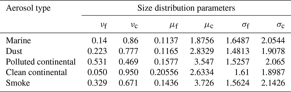
Here, S_V is called the volume scaling factor and is estimated from the ratio of α, the CALIOP-derived extinction coefficient, and α_n, the extinction coefficient calculated from the normalized size distribution and refractive index using MOPSMAP. For modelling α_n, we treat continental (clean continental, polluted continental, and smoke) and marine aerosols as spheres and use Mie scattering theory. We consider desert dust aerosols as spheroids and use a combination of the T matrix and the improved geometric optics method, depending on the value of the aerosol size parameter, to model α_n. The values of normalized size distribution parameters, such as the standard deviation (σ_i), volume fraction (ν_i), and mean radius (μ_i) of ith (fine and coarse) mode, are listed in the Table A1. After the scaling step, the volume size distribution is converted to a number size distribution, which is then integrated starting at 50 nm to compute n_50,dry for continental and marine aerosols and at 100 nm to compute n_100,dry for desert dust aerosols. This is because aerosols within these size ranges have been identified to act as CCN for a supersaturation of 0.15 %–0.20 % in several studies using in situ measurements (Koehler et al., 2009; Rose et al., 2010; Deng et al., 2011; Kumar et al., 2011; Mamouri and Ansmann, 2016). In accordance with the Aerosol Robotic Network (AERONET) size distributions, the upper radius limit for integrating the size distributions is set at 15 µm. Further, the CCN concentrations at higher supersaturation can be estimated following the simple CCN parameterization given by Mamouri and Ansmann (2016):

$$\begin{array}{}\text{(2)}& n_{\mathrm{CCN}}=f_{\mathrm{ss}}\cdot n_{j,\mathrm{dry}},\end{array}$$

where j represents the lower radius limit of the size-distribution integration and f_ss is the enhancement factor with values equal to 1.0, 1.35, and 1.7 for supersaturations of 0.15 %–0.20 %, 0.25 %, and 0.40 %, respectively. While the simple parameterizations based on aerosol size and type do not consider the aerosol chemistry stringently, they have been shown to yield reasonable n_CCN estimates, particularly when applied to spaceborne lidar measurements (Choudhury and Tesche, 2022a, b). Further information on the limitations and known issues of the algorithm are discussed in Sect. 3.3.

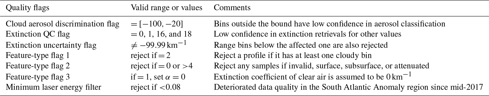
Table 1 Quality screening applied to the CALIPSO Level 2 Aerosol Profile product.

3 Methodology

In this section, we discuss the complete methodology used to apply the CCN retrieval algorithm to the CALIPSO profile data to generate a global gridded monthly CCN data set. It includes a number of preprocessing stages that are implemented prior to applying the CCN retrieval algorithm, followed by a set of post-processing steps to convert the n_CCN profiles to global gridded data.

3.1 Preprocessing

3.1.1 Quality screening

The CALIPSO Level 2 Aerosol Profile product includes a number of quality control flags that are intended to filter out unreliable retrievals that may result from clouds misclassified as aerosols and errors pertaining to the extinction coefficient retrieval (Tackett et al., 2018). The cloud–aerosol discrimination (CAD) score specifies the confidence in the classification of aerosol and cloud for each data bin (Liu et al., 2009). We only select data which have a CAD score in the range [−100, −20], as they correspond to a high confidence in the aerosol classification (Liu et al., 2009). To screen retrievals with extinction-coefficient-related retrieval issues, we use the “extinction uncertainty” and the “extinction QC” (extQC) metrics. Data bins with an extinction uncertainty of −99.99 km are not considered and nor are the bins present below them, as the extinction retrieval uncertainty may propagate to solutions at lower altitudes. The extQC flag describes how the extinction coefficient is generated for each Level 2 sample. Following Tackett et al. (2018), we only consider bins with extQC values of 0, 1, 16, and 18, because they represent high confidence in the retrieved extinction coefficient. We also use the minimum laser energy (MLE) parameter at 532 nm, which was recently introduced in the version 4.20 update, to identify and screen columns affected by low-laser-energy shots (MLE <0.08) that result in higher noise and degraded retrieval quality. Additionally, we filter out the profiles or columns with cloudy pixels, as clouds can impede aerosol retrievals underneath them due to signal attenuation. All of the quality-screening criteria used in this work are listed in Table 1. Readers are advised to refer to Tackett et al. (2018) for further information on the production and functions of the quality-screening flags.

3.1.2 Dust separation

Before applying the CCN retrieval algorithm to the quality-screened Level 2 data, the extinction coefficients of dust mixtures (polluted dust and dusty marine) need to be separated into dust and non-dust components. This is done by using the particle depolarization ratio and first separating the backscatter coefficient into dust and non-dust components following the methodology described in Tesche et al. (2009). We assume the aerosol mixture to be pure dust (non-dust) if the particle depolarization ratio is >0.31 (<0.05). The backscatter coefficients of aerosol mixtures with a depolarization ratio between 0.05 and 0.31 are separated using Eq. (14) of Tesche et al. (2009). This is a rather straightforward technique that assumes aerosols to be externally mixed. It has been implemented and tested in several studies based on ground-based and spaceborne lidar retrievals (Mamouri and Ansmann, 2015, 2016; Choudhury et al., 2022; Choudhury and Tesche, 2022b). The extinction coefficients of dust and non-dust aerosol components are then estimated by multiplying the respective separated backscatter coefficients by the lidar ratios corresponding to the aerosol type. Following this methodology, the polluted dust aerosol mixture is separated into polluted continental and desert dust components, and the dusty marine aerosol mixture is separated into desert dust and marine components. The lidar ratio for these aerosol types is taken from Table 2 of Kim et al. (2018).

3.1.3 Hygroscopicity correction

Hydrophilic aerosols may grow in size under moist conditions and, thus, may result in a higher extinction coefficient relative to dry conditions, even if the aerosol number concentrations remains the same (Zieger et al., 2013). Further, the normalized size distributions used in OMCAM have been derived mostly under dry conditions (Omar et al., 2009), and the CCN parameterization requires the dry-aerosol number concentration. Therefore, the extinction coefficient is first corrected for aerosol hygroscopicity before applying the OMCAM algorithm. This is done by using the aerosol-type-specific growth factors (ratio of ambient and dry extinction coefficients) given in Choudhury et al. (2022) at different RH values. The growth factors for continental and marine aerosols are estimated at different RH values using the κ parameterization (Petters and Kreidenweis, 2007), which expresses the hygroscopic growth of an aerosol particle with a dry radius r_dry in terms of a hygroscopicity parameter κ as follows:

$$\begin{array}{}\text{(3)}& {\displaystyle \frac{r_{\mathrm{wet}}\left(\mathrm{RH}\right)}{r_{\mathrm{dry}}}}=(\mathrm{1}+\mathit{\kappa }\cdot {\displaystyle \frac{\mathrm{RH}}{\mathrm{1}-\mathrm{RH}}}{)}^{\frac{\mathrm{1}}{\mathrm{3}}}.\end{array}$$

Here, r_wet is the wet radius of a particle at a given relative humidity (RH). The ratio between r_wet and r_dry is used to modify the dry normalized size distributions of aerosols at different RH values, followed by the computation of their respective extinction coefficients using the MOPSMAP package. A globally averaged κ value of 0.3 is used for polluted continental, clean continental, and smoke aerosols, whereas a value of 0.7 is used for marine aerosols (Andreae and Rosenfeld, 2008). We treat desert dust as non-hygroscopic and do not modify the extinction coefficients for dust samples. This approach has been shown to yield dry extinction coefficients and dry number concentrations that are consistent with in situ measurements (Choudhury et al., 2022; Choudhury and Tesche, 2022a). Further details on the hygroscopicity correction are given in Choudhury et al. (2022).

3.2 Post-processing

We use the quality-screened CALIPSO Level 2 data obtained by following the steps outlined in Sect. 3.1.1 in the OMCAM algorithm to estimate n_CCN profiles at a supersaturation of 0.20 %. We further limit the n_CCN in the output data to a supersaturation of 0.20 %, as it can be easily converted to higher supersaturations by using the enhancement factors as shown in Eq. (2). In this section, we discuss the spatial and temporal grid configuration used to covert the n_CCN profiles to 3D gridded data. We further describe all of the parameters stored in the output data files.

3.2.1 Gridding, sampling, and averaging

The CALIPSO Level 2 Aerosol Profile data have a very high vertical resolution of 60 m and an along-swath resolution of 5 km. However, because of the negligible divergence of lasers, CALIPSO has a narrow cross-track coverage. Further, the distance between two consecutive overpasses is inversely proportional to the latitude because of CALIPSO's polar orbit with an inclination of 98.36^∘. Therefore, a grid box of a certain dimension close to the Equator will include fewer overpasses compared with one close to the poles. Due to this factor and to produce a regionally representative global gridded data with a sufficient aerosol sampling frequency in each grid cell, we choose a monthly temporal resolution and a horizontal grid resolution of $\mathrm{2}{}^{\circ }\times \mathrm{5}{}^{\circ }$ to process the n_CCN profiles. The vertical resolution is, however, kept unchanged at 60 m. We further consider both the daytime and night-time CALIPSO overpasses to compute the average n_CCN to increase the sampling frequency. This grid configuration is also used in monthly CALIPSO Level 3 products (Tackett et al., 2018) and is suggested by Choudhury and Tesche (2022b) to compile a global n_CCN data set. Using this grid, we estimated the number of days observed with valid n_CCN (value ≥0; hereafter abbreviated as NDO) samples in each grid box for each month and found them to be as high as 17 d in the tropics and 31 d at the poles. Note that the NDO estimated here is different from the “Days_Of_Month_Observed” parameter in the CALIPSO Level 3 product, as the latter also considers valid cloud retrievals.

We further produced a climatological n_CCN data set using the same horizontal and vertical grid configuration. An alternative approach would be to consider a higher horizontal resolution of $\mathrm{1}{}^{\circ }\times \mathrm{1}{}^{\circ }$, as used in Amiridis et al. (2015), to construct a climatology of aerosol and cloud properties using the CALIPSO Level 2 data. However, using such a grid results in low aerosol sampling, especially in the tropics. This is shown in Fig. 1 based on more than 15 years of CALIPSO measurements. While the former gives a maximum of 2340 d observed in the tropics, the latter results in a significantly lower maximum of 591 d. Therefore, we use the coarser grid to produce the n_CCN climatology that ensures the ample aerosol sampling required for a realistic and regionally representative data set.

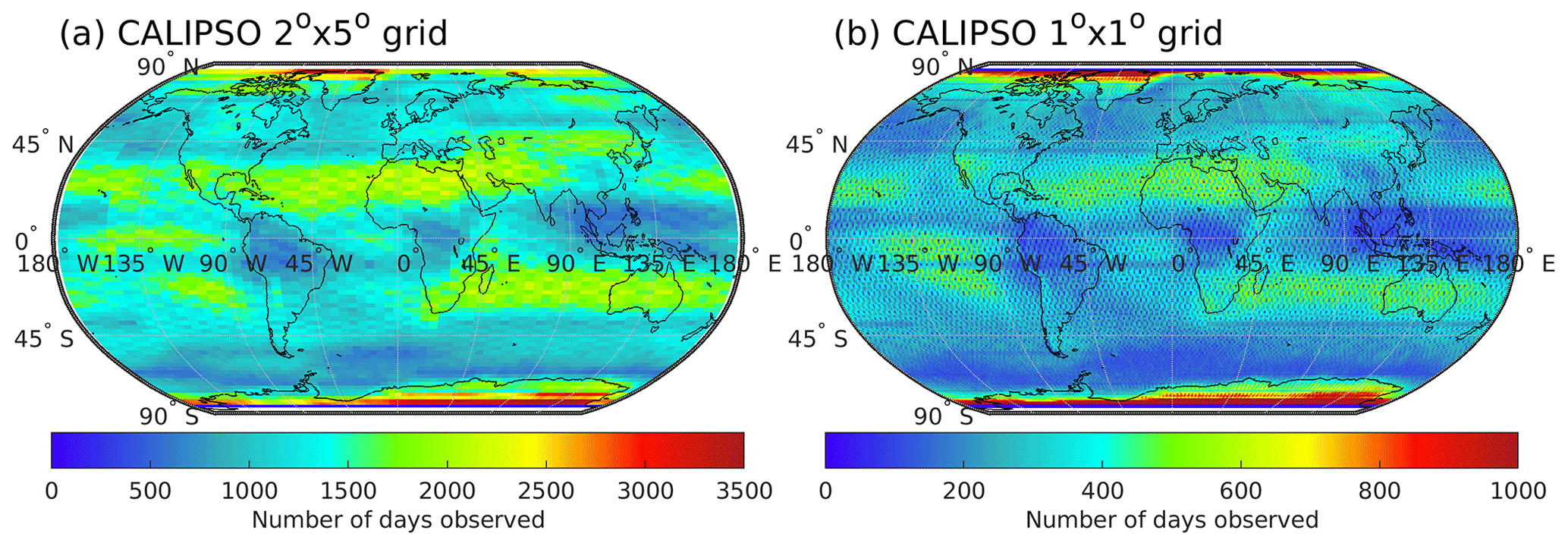
Figure 1 Global map of the number of days with valid CCN observations (n_CCN≥0 cm⁻³) for horizontal grid configurations of $\mathrm{2}{}^{\circ }\times \mathrm{5}{}^{\circ }$ (a) and $\mathrm{1}{}^{\circ }\times \mathrm{1}{}^{\circ }$ (b) produced from more than 15 years of CALIOP measurements.

For averaging the n_CCN for each latitude, longitude, and altitude grid cell, we follow the methodology used in Tackett et al. (2018) for producing the CALIPSO Level 3 aerosol products. We assign the clear-air Level 2 bins with an extinction coefficient of 0 km⁻¹, which leads to an n_CCN of 0 cm⁻³, and compute the average n_CCN ($\stackrel{\mathrm{‾}}{n_{\mathrm{CCN}}}$) for each grid cell as follows:

$$\begin{array}{}\text{(4)}& \stackrel{\mathrm{‾}}{n_{\mathrm{CCN}}}={\displaystyle \frac{{\sum }_{i=\mathrm{1}}^{N_{\mathrm{a}}}{n}_{\mathrm{CCN},i}}{N_{\mathrm{a}}+N_{\mathrm{ca}}}}.\end{array}$$

Here, N_a is the number of Level 2 samples with an aerosol extinction coefficient > 0 km⁻¹ and N_ca is the number of clear-air samples. This averaging scheme is used to generate the global monthly gridded data set as well as the n_CCN climatology.

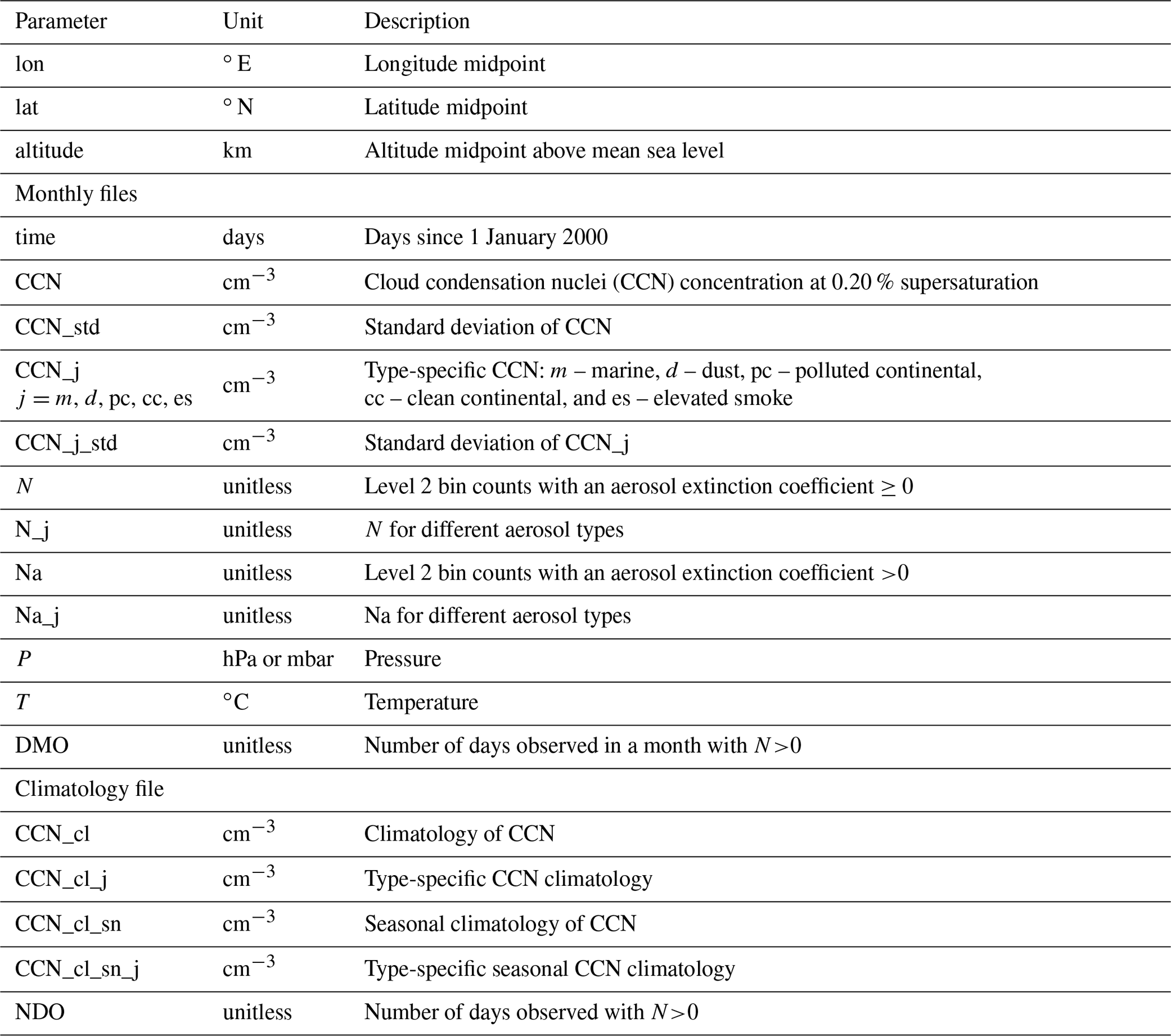
3.2.2 Output data records

Following the gridding and averaging scheme discussed in the previous section, we produce the global n_CCN data sets at a monthly temporal resolution. Table 2 provides a list of all of the parameters included in the output data and their description. Along with the averaged n_CCN, we further provide the total number of Level 2 samples with an aerosol extinction coefficient ≥ 0 km⁻¹ ($N=N_{\mathrm{a}}+N_{\mathrm{ca}}$) and with an extinction coefficient > 0 (N_a). The n_CCN, N, and N_a are also provided separately for each aerosol type. Note that both N and N_a may not be equal to the sum of the contributions from all of the aerosol types, specifically when aerosol mixtures are present. They are useful in computing annual and seasonal averages of n_CCN using Eq. (4). We further provide the NDO for each month and suggest using the data only when NDO > 10 (coverage of a minimum of 30 % of days a month). Average pressure and temperature are also provided for each latitude, longitude, and altitude grid cell. The pressure values can be used to convert the data from height coordinates to pressure coordinates. As the retrievals over an altitude of 8 km constitute about 0.7 % of the total tropospheric CCN, all parameters are limited to a maximum altitude of 8 km in order to reduce the overall data size. For ease of accessibility across different platforms, we provide the data in Network Common Data Form (NetCDF) format with a medium level of data compression (deflate level of 5). These NetCDF files are accessible at https://doi.org/10.1594/PANGAEA.956215 (Choudhury and Tesche, 2023) and are tested to work with tools and software like Climate Data Operators (CDO), netCDF Operators (NCO), and ncdump. The netCDF files with monthly gridded data are provided separately for each year from 2006 to 2021. The n_CCN climatology is provided in a separate netCDF file, with a data structure and nomenclature similar to the monthly data. The file also includes n_CCN climatologies for the boreal winter (December, January, and February), spring (March, April, and May), summer (June, July, and August), and autumn (September, October, and November) seasons.

Table 2 Description of the NetCDF data records.

3.3 Uncertainty, known issues, and validation

The uncertainty in the estimated n_CCN can arise from the uncertainties in the input parameters, such as the aerosol extinction coefficient, type-specific normalized size distribution, and the ambient RH, as well as from the dust-separation technique and the CCN parameterizations used in the algorithm. Choudhury and Tesche (2022a) studied the sensitivity of the cloud-relevant aerosol number concentrations (n_j,dry) to the variations in the size distributions for each aerosol type at different RH values. They reported a variation of a factor of 1–1.5 depending on the aerosol type. Combining this with the uncertainties associated with other previously mentioned sources, the overall uncertainty associated with the output n_CCN is found to be between a factor of 2 and 3. Such a range is reasonable for the spaceborne retrieval of n_CCN (Shinozuka et al., 2015; Mamouri and Ansmann, 2016), as atmospheric CCN concentrations can potentially vary by orders of magnitude in space and time (Schmale et al., 2018).

There are some known issues associated with CALIOP's retrieval algorithm and the CCN parameterizations used to produce the global data set. First, faint aerosol layers with an extinction coefficient <0.001 km⁻¹ (optical depth <0.01) may not exceed the signal-to-noise ratio required to be detected by CALIOP (Tackett et al., 2018; Mao et al., 2022). The background noise due to solar radiation further impacts the feature detection, especially for the daytime retrievals (Winker et al., 2009, 2013). Such layers may therefore be classified as clear air by CALIOP's feature classification algorithm and assigned with a zero extinction coefficient. This may result in an underestimation of the average extinction and, thus, the n_CCN, particularly in grid cells comprising a clean environment (rural continental sites and higher altitudes). Second, the simple aerosol-type-specific parameterizations implemented in this study assume that all particles over a certain minimum radius are CCN active. This may lead to an overestimation of n_CCN that may also compensate for the underestimation due to the undetected aerosol layers. Third, CALIOP cannot distinguish between polluted continental and smoke aerosol layers that occur below a layer-top height of 2.5 km (Kim et al., 2018). Therefore, isolated smoke layers that do not extend above a height of 2.5 km may get classified as polluted continental aerosols, leading to an overestimation of n_CCN by about 13.6 %. As a result, we anticipate that the CCN retrieval algorithm will overestimate the CCN in areas often influenced by smoke aerosols below 2.5 km. Additionally, strong signal attenuation caused by optically thick aerosol layers located above may lead to increased uncertainties in the retrievals of layers below. Nevertheless, it is anticipated that these retrievals will be filtered out during the quality-screening process.

As mentioned earlier in Sect. 3.2.1, we combine daytime and night-time CCN retrievals to achieve an optimal sampling frequency. The daytime retrievals usually have a lower signal-to-noise ratio compared with night-time retrievals, which may result in higher retrieval uncertainty (Young et al., 2013; Tackett et al., 2018). By comparing the daytime and night-time CCN climatology (refer to Fig. S1 in the Supplement), we observe higher values over continents in the former. This observation is expected because anthropogenic emissions are more prominent during the day. The values over oceans are comparable in both cases. However, it is important to note that this concurrence may be attributed to long-term averaging used in computing the climatologies. Therefore, a more detailed comparison is required at various temporal scales (instantaneous, monthly, seasonal, and annual) to accurately quantify the effect of merging daytime and night-time retrievals. Such an investigation is beyond the scope of the present study and will be a subject of future analysis.

The n_CCN values estimated using the OMCAM algorithm have been validated using independent ground-based and airborne in situ measurements for different aerosol environments (Choudhury et al., 2022; Choudhury and Tesche, 2022b; Aravindhavel et al., 2023). Even though the uncertainty associated with the CCN retrieval from CALIOP can be as high as a factor of 3, the validation results indicate a very good agreement with in situ measurements, with a normalized mean bias of ≈22 % and a correlation coefficient of ≈0.7. Such consensus has not yet been achieved for spaceborne estimations of aerosol and CCN number concentrations, accentuating the potential of the spaceborne-lidar-derived global n_CCN data set.

4 Results

4.1 Comparison with global model outputs

A comparison of the CALIOP-estimated average global n_CCN with the model outputs for the year 2011 is shown in Fig. 2. Excluding the data within the Antarctic Circle (latitudes $<-\mathrm{66.5}$^∘ N), CALIOP-estimated CCN concentrations are, on average, larger than the models, with a normalized difference ($\mathrm{100}\times (\mathrm{MODEL}-\mathrm{CALIOP})/\mathrm{CALIOP}$) of −65.6 %, 89.4 %, and 4.5 % for the median, minimum, and maximum of all of the models, respectively. The larger values are expected, as the models have been identified to underestimate the n_CCN when compared with in situ measurements at continental surface stations with a mean error of 60 % (Fanourgakis et al., 2019a). The best agreement with CALIOP is found for the maximum of all of the models, particularly in the Northern Hemisphere. For retrievals over the Southern Ocean with latitudes <45^∘ S, the modelled n_CCN are significantly lower than that of CALIOP with a maximum of 171.9 cm⁻³. Recent in situ measurements show that the n_CCN in such regions can even exceed 500 cm⁻³ (Humphries et al., 2021), which is not observed in the model outputs, although it is well captured by CALIOP. This highlights the potential of the CALIOP-derived global n_CCN data set to validate model outputs at locations where in situ observations are sparse or even non-existent. Please note that the comparison presented here is intended to highlight the data set's unique potential for application and that validation studies have already been published (Choudhury et al., 2022; Choudhury and Tesche, 2022b; Fanourgakis et al., 2019a). Readers are encouraged to use the full potential of the open-source data set to conduct further comprehensive model evaluation studies.

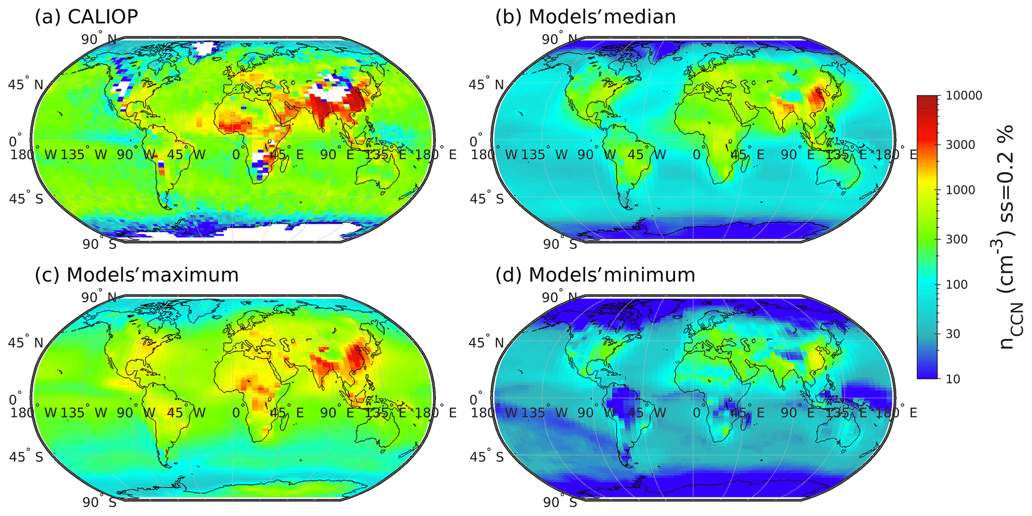
Figure 2 Comparison of global n_CCN maps at a supersaturation of 0.20 % estimated from CALIOP between altitudes of 500 m and 1 km (a) and from the outputs of 15 global models at the surface (b–d) for the year 2011. Panels (b), (c), and (d) represent the median, maximum, and minimum modelled n_CCN, respectively.

4.2 CCN climatology

Figure 3 shows the global n_CCN climatology computed from the monthly data set averaged for altitudes below 2 km using Eq. (4) and the corresponding averaged n_CCN profile. The global average n_CCN is estimated to be 365.12±649.92 cm⁻³, with 683.25±1172.95 cm⁻³ over land and 303.2±382.33 cm⁻³ over ocean. The highest concentrations are found over regions influenced by pollution and dust aerosols, such as South and East Asia. Polluted continental aerosols with an average n_CCN of 124.3±459 cm⁻³ have the maximum contribution to the total CCN below 2 km, followed by marine (110.8±175.12 cm⁻³), dust (108.9±256.39 cm⁻³), and elevated smoke (21±74.61 cm⁻³) aerosols. Clean continental aerosols with a global average of 0.12±0.34 cm⁻³ contribute the least to the total CCN (not shown). Over land, the average CCN value is estimated to be 683.25±1172.95 cm⁻³, with maximum contributions coming from polluted continental (419.4±900.9 cm⁻³), dust (203.67±435.45 cm⁻³), and smoke (43.6±117.93 cm⁻³) aerosols. The concentrations over oceans are less than half of those over land with an average of 303.2±382.33 cm⁻³, with marine (181.93±221.2 cm⁻³), dust (84.68±206.8 cm⁻³), and polluted continental (27.33±114.17 cm⁻³) aerosols being the major contributors. Although pollution aerosols contribute the most to the total CCN, it is evident that dust has the most widespread coverage, encompassing nearly the entire globe, indicating its significance in ACIs, even in pristine aerosol environments far away from the continents.

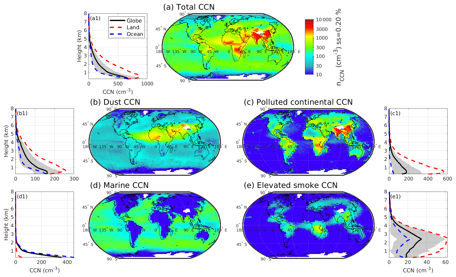
Figure 3 Global climatology of n_CCN at a supersaturation of 0.20 % estimated from the monthly CCN data set averaged for altitudes below 2 km for all aerosol types (a), and the results separated according to mineral dust (b), polluted continental (c), marine (d), and elevated smoke (e) aerosol types, respectively. The sub-panels adjacent to each panel depict the vertical variation in n_CCN averaged over the globe (solid black line), land (dashed red line), and ocean (dashed blue line). The semitransparent grey patch represents half of the standard deviation in globally averaged n_CCN.

When considering the vertical distribution of n_CCN, the highest values are observed near the surface, and these values decrease exponentially as the altitude increases. The majority of marine CCN (97 %) and continental CCN (78 %) are predominantly located at altitudes below 2 km. On the other hand, smoke and dust CCN extend into the free troposphere, with approximately 60 % and 33 % located above 2 km altitude, respectively. Interestingly, smoke CCN exhibit an opposite trend, with concentrations increasing with height and reaching a maximum between 2 and 3 km before decreasing at higher altitudes. Land-based aerosols make up the majority of free-tropospheric CCN, with 68 % located above 2 km, compared with 32 % for aerosols over oceans. They exhibit a relatively higher contribution to the global CCN across all altitude levels. It is important to note that this variation may not be observed in localized regions over oceans that are more frequently affected by dust and smoke transported from nearby continents, for instance, the west of Africa.

4.2.1 Seasonal climatology

Figure 4 illustrates the global map presenting the seasonal climatologies of total n_CCN for altitudes below 2 km, along with the corresponding profiles of spatially averaged type-specific n_CCN. The global average n_CCN reaches its maximum during winter with a value of 376±800.91 cm⁻³. Similar to the global climatology in Fig. 4, the average winter n_CCN is significantly higher over land (725.53±1499.36 cm⁻³) compared with over ocean (321.61±427.20 cm⁻³). Strong seasonality in n_CCN is observed in regions influenced by Northern Hemisphere summer monsoon, such as Asia and West Africa, with minimum values occurring during the summer. This pattern is likely attributed to the wet scavenging of aerosol particles associated with cloud droplet formation and precipitation during the monsoon season. The seasonality of n_CCN is also evident in regions like East and Central Africa, possibly resulting from changes in local biomass burning patterns (Myhre et al., 2003; van der Werf et al., 2017) that peak during the dry summer (Southern Hemisphere winter) season.

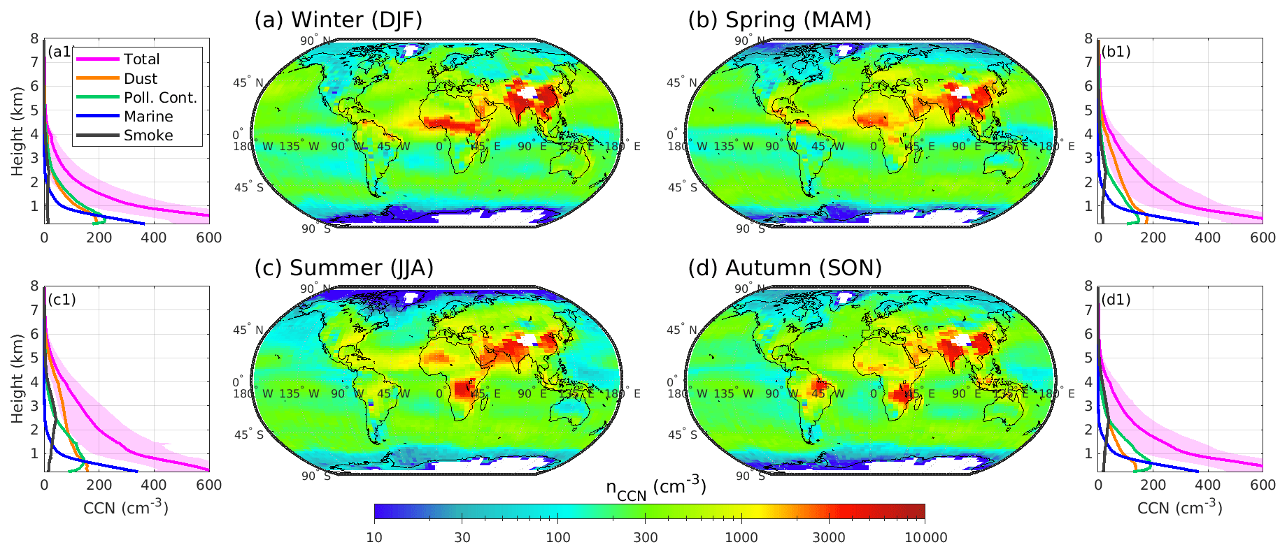
Figure 4 Seasonal climatology of n_CCN at a supersaturation of 0.20 % and at altitudes below 2 km for winter (a), spring (b), summer (c), and autumn (d). The vertical variation in seasonal n_CCN is depicted in the adjacent sub-panels for dust (orange line), polluted continental (green line), marine (blue line), and smoke (black line) aerosol types. The magenta profile in the sub-panels represent the total n_CCN, and the semitransparent patch highlights the associated standard deviation scaled to half of its original value for better visualization.

Furthermore, seasonality in the n_CCN profiles is observed for all of the aerosol types, except for marine aerosols. During boreal winter, CCN concentrations are predominantly limited to altitudes below 2–3 km (84 %–94 %), with the highest near-surface concentrations compared with other seasons. The vertical distribution of CCN for all of the aerosol types gradually expands to higher altitudes with the transition to warmer spring and summer seasons. Although near-surface n_CCN are at their lowest during summer, they contribute the most to the free-tropospheric CCN, accounting for 35 % of CCN at altitudes higher than 2 km. This is followed by spring (29 %), autumn (24 %), and winter (16 %), highlighting the substantial impact of the boundary layer depth on modulating the vertical extent of CCN throughout all seasons.

It is worthwhile noting that, in Figs. 3 and 4, we have limited our focus to the spatial variations in low-level aerosols (altitude <2 km) and have only presented the profiles of spatially averaged n_CCN. The climatology data include information up to an altitude of 8 km for various aerosol types, which offers a unique opportunity to investigate the altitudinal variations in type-specific n_CCN across different seasons and regions throughout the globe. Such studies, however, are outside the scope of this paper, which is aimed at introducing a new global CCN data set, and will be the focus of a future publication.

5 Code and data availability

The CALIPSO Level 2 Aerosol Profile product can be downloaded from https://doi.org/10.5067/CALIOP/ (NASA/LARC/SD/ASDC, 2018). The data produced in this work are available at https://doi.org/10.1594/PANGAEA.956215 (Choudhury and Tesche, 2023). The model data used for comparison can be found at https://doi.org/10.5281/zenodo.3265866 (Fanourgakis et al., 2019b). The codes used to generate the data were written in MATLAB and can be provided by the corresponding author upon reasonable request. The MATLAB script used to generate the plots shown in the paper is provided in the Supplement.

6 Conclusion and usage notes

We present a first aerosol-type-specific global CCN data set derived from spaceborne lidar measurements at a horizontal latitude–longitude resolution of $\mathrm{2}{}^{\circ }\times \mathrm{5}{}^{\circ }$, a vertical resolution of 60 m, and a temporal resolution of 1 month. The data set spans more than 15 years, from June 2006 to December 2021, or a total of 186 months. We further use the complete time series to construct a global n_CCN climatology for different aerosol types. The climatologies are also reported at a seasonal timescale. These data sets are aimed at replacing the currently used satellite-derived optical proxies for CCN. Readers are encouraged to utilize the full potential of the global data set for the following purposes:

• The data can be used to investigate the horizontal and vertical distributions of CCN for various aerosol types as well as to study their trends and variations across monthly, seasonal, and annual timescales. In Sect. 4.2 of this paper, we briefly discuss the spatial distribution of n_CCN for different aerosol types for altitudes limited below 2 km, where we find the global average n_CCN to be 365.12 cm⁻³ and identify various CCN hotspots. This approach can be expanded to include the variations along the height and time dimensions. In addition, the type-specific CCN concentrations can be used to identify the sources and sinks of CCN as well as to investigate the contributions of the long-range transport of aerosols with a high residence time (e.g. dust and smoke) to CCN in the atmosphere.

• Recent studies have demonstrated that spaceborne aerosol, cloud, and radiation measurements at a monthly temporal resolution can be used to estimate the radiative forcing associated with ACIs (Wall et al., 2022; Chen et al., 2022). The monthly data presented in this paper can be similarly coupled with cloud and radiation measurements to quantify ACIs. Studies have demonstrated the effectiveness of CALIOP in even retrieving height-resolved cloud microphysical properties (Zhang et al., 2019; Zang et al., 2021), which can be directly coupled with corresponding CCN estimates to investigate ACIs. Furthermore, the type-specific CCN data can be used to accurately quantify the anthropogenic component of present-day CCN (sum of polluted continental and smoke components), which has previously been estimated from model simulations of past climate (Bellouin et al., 2020; Quaas et al., 2020). This creates a unique opportunity to quantify ACIs by solely using satellite observations independent of model simulations.

• Due to the lack of any observation-based global CCN data, model evaluation studies usually rely on in situ measurements, which are only available for a limited time period at certain point locations. Further, the observations over oceans and the height-resolved measurements restricting the model evaluation to specific land sites are sparse. However, validating global model outputs with respect to estimating height-resolved CCN concentrations over both land and ocean is necessary, as they form the key components of ACIs and, thus, the future climate predictions. With the height-resolved CCN data available for more than 15 years, a comprehensive model evaluation can be performed at different height levels, even for regions over oceans far from continents. In Sect. 4.1 of the paper, we compare the annual average n_CCN estimated from the monthly data with the simulations from 15 global climate models at the surface for the year 2011, highlighting the data's usefulness with respect to assessing model outputs. This idea can be further expanded to other models by incorporating the temporal and altitudinal distribution of CCN for different aerosol types encompassing a longer time span.

The above list is by no means exhaustive. Users can also use this data set and check for closure with other spaceborne retrievals of cloud-relevant CCN or aerosol number concentrations. For instance, comparisons can be made with (i) column-integrated aerosol number concentrations derived from polarimetric observations (Hasekamp et al., 2019), (ii) aerosol number and CCN concentrations estimated from spaceborne lidar using AERONET-derived extinction-to-number concentration conversions (Mamouri and Ansmann, 2016), (iii) CCN at cloud base derived from passive spaceborne sensors by treating clouds as CCN chambers (Rosenfeld et al., 2016), or with any future algorithms or data.

Appendix A

Table A1 Lognormal, bimodal volume size distribution parameters of different aerosol types. ν, μ, and σ represent the volume fraction, mode radius, and standard deviation, respectively. The subscripts “f” and “c” represent the fine and coarse modes of the size distribution, respectively.