A monthly 1° resolution dataset of daytime cloud fraction over the Arctic during 2000–2020 based on multiple satellite products

The low accuracy of satellite cloud fraction (CF) data over the Arctic seriously restricts the accurate assessment of the regional and global radiative energy balance under a changing climate. Previous studies have reported that no individual satellite CF product could satisfy the needs of accuracy and spatiotemporal coverage simultaneously for long-term applications over the Arctic. Merging multiple CF products with complementary properties can provide an effective way to produce a spatiotemporally complete CF data record with higher accuracy. This study proposed a spatiotemporal statistical data fusion framework based on cumulative distribution function (CDF) matching and the Bayesian maximum entropy (BME) method to produce a synthetic 1^∘ × 1^∘ CF dataset in the Arctic during 2000–2020. The CDF matching was employed to remove the systematic biases among multiple passive sensor datasets through the constraint of using CF from an active sensor. The BME method was employed to combine adjusted satellite CF products to produce a spatiotemporally complete and accurate CF product. The advantages of the presented fusing framework are that it not only uses the spatiotemporal autocorrelations but also explicitly incorporates the uncertainties of passive sensor products benchmarked with reference data, i.e., active sensor product and ground-based observations. The inconsistencies of Arctic CF between passive sensor products and the reference data were reduced by about 10 %–20 % after fusing, with particularly noticeable improvements in the vicinity of Greenland. Compared with ground-based observations, R² increased by about 0.20–0.48, and the root mean square error (RMSE) and bias reductions averaged about 6.09 % and 4.04 % for land regions, respectively; these metrics for ocean regions were about 0.05–0.31, 2.85 %, and 3.15 %, respectively. Compared with active sensor data, R² increased by nearly 0.16, and RMSE and bias declined by about 3.77 % and 4.31 %, respectively, in land; meanwhile, improvements in ocean regions were about 0.3 for R², 4.46 % for RMSE, and 3.92 % for bias. The results of the comparison with ERA5 and the Meteorological Research Institute – Atmospheric General Circulation model version 3.2S (MRI-AGCM3-2-S) climate model suggest an obvious improvement in the consistency between the satellite-observed CF and the reanalysis and model data after fusion. This serves as a promising indication that the fused CF results hold the potential to deliver reliable satellite observations for modeling and reanalysis data. Moreover, the fused product effectively supplements the temporal gaps of Advanced Very High Resolution Radiometer (AVHRR)-based products caused by satellite faults and the data missing from MODIS-based products prior to the launch of Aqua, and it extends the temporal range better than the active product; it addresses the spatial insufficiency of the active sensor data and the AVHRR-based products acquired at latitudes greater than 82.5^∘ N. A continuous monthly 1^∘ CF product covering the entire Arctic during 2000–2020 was generated and is freely available to the public at https://doi.org/10.5281/zenodo.7624605 (Liu and He, 2022). This is of great importance for reducing the uncertainty in the estimation of surface radiation parameters and thus helps researchers to better understand the Earth's energy imbalance.

1 Introduction

Clouds substantially affect Earth's energy budget by reflecting solar radiation back to space and by restricting emissions of thermal radiation into space (Ramanathan et al., 1989; Van Tricht et al., 2016; Danso et al., 2020). Clouds are also an essential variable in the climate system, because they are directly associated with precipitation and aerosol loading (Toll et al., 2019; Poulsen et al., 2016). The cloud fraction (CF), which represents the amount of sky estimated to be covered by a specified cloud type or level (partial CF) or by all cloud types and levels (total CF), has long been recognized as a major source of uncertainty when estimating radiation flux and future climate change (Xie et al., 2010; Y. Liu et al., 2011; Qian et al., 2012; Danso et al., 2020). An accurate representation of CF is essential for the evaluation of regional and global energy budgets as well as for predicting future climatic conditions. However, variances in CF definitions and system differences commonly exist among different sources of data. As a solution, the fused product provides a higher level of definition consistency and accuracy in comparison to alternative datasets.

By making spatially continuous observations, satellites provided us with an unprecedented advantage in assessing regional and global cloud effects. In the last few decades, increased effort has been made to develop, analyze, and validate global or regional cloud property datasets that are based on long-term satellite observations (Heidinger et al., 2014; Hollmann et al., 2013; Karlsson and Devasthale, 2018; Marchant et al., 2016; Rossow and Schiffer, 1999; Stubenrauch et al., 2013; Enriquez-Alonso et al., 2016; Sun et al., 2015; Tzallas et al., 2019; Wu et al., 2014). Studies have also shown that although different cloud datasets were derived from different observation instruments and algorithms, most of them provide quite consistent CF observations in middle- and lower-latitude regions (Karlsson and Devasthale, 2018; Stengel et al., 2017; Claudia et al., 2012). However, systematic errors and artifacts exist in CF data, so some inconsistencies inevitably occur among different datasets (Sun et al., 2015; Tzallas et al., 2019; Wu et al., 2014), especially in the polar regions (Liu et al., 2022). Perennial snow/ice coverage coupled with frequent moisture inversions in the Arctic has limited the cloud detection capabilities of passive sensor datasets, where the differences between these various datasets tend to be about 2-fold in magnitude when compared with datasets acquired at other latitudes (Karlsson and Devasthale, 2018; Liu et al., 2022; Stubenrauch et al., 2013). The uncertainties of the annual global surface downward longwave (LW) and shortwave (SW) fluxes caused by satellite-derived cloud properties were calculated at about 2 % (7 and 4 W m⁻², respectively), and those for global surface upward LW and SW fluxes were about 0.8 % (about 3 W m⁻²) and 13 % (also 3 W m⁻²), respectively (Kato et al., 2011, 2012; Kim and Ramanathan, 2008). It should be noted that the differences in CF may have a more obvious impact on the surface radiation budget in high-latitude polar regions. Kennedy et al. (2012) found that the CF bias might cause monthly biases in Arctic surface SW and LW fluxes over 90 and 60 W m⁻² for some reanalyses, respectively (Kennedy et al., 2012). Walsh et al. (2009) proposed that the bias of summer low-level CF would create deviations of about 160 W m⁻² in estimated SW radiation (Walsh et al., 2009). Some other related studies have also found that the variances of annual Arctic surface radiation estimation caused by CF uncertainty were higher than 10 W m⁻² (Hakuba et al., 2017; Kato et al., 2018b; Huang et al., 2017). Therefore, relying on a single CF dataset may introduce large uncertainty when analyzing the cloud dynamics over the Arctic, further affecting the estimated energy budget and related climate applications.

Each cloud dataset has its own advantages and disadvantages in Arctic CF detection. The Advanced Very High Resolution Radiometer (AVHRR) offers the longest continuous satellite observation records extending from 1978 to the present and provides daily global coverage based on data from several AVHRR instruments. With the successful operation of new generations of satellites, the frequency of the global view has increased to more than eight each day, which provides richer angular information for CF observations (Heidinger et al., 2014; Karlsson et al., 2017). Many cloud products exist that are based on AVHRR sensors. The International Satellite Cloud Climatology Project (ISCCP) H-series product relies on newer passive imagers with higher spectral, spatial, radiometric, and temporal resolutions; it provides revised daytime cloud detection over snow and ice in polar regions (Young et al., 2018). Moreover, the ISCCP is largely unaffected by the AVHRR orbital drifts (Loyola R et al., 2010; Liu et al., 2022). The CM SAF cLoud, Albedo, and RAdiation datasets (CLARA-A1/A2) systematically use CALIPSO-CALIOP (Cloud-Aerosol LIdar with Orthogonal Polarization) cloud information for development and validation purposes, and it optimizes the detection conditions during the polar day over snow- and ice-covered surfaces (Karlsson et al., 2017; Karlsson and Håkansson, 2018). The AVHRR Pathfinder Atmospheres–Extended (PATMOS-x) product is the first multi-parameter dataset that is making use of all AVHRR channels. This product has a relatively finer spatial resolution than other AVHRR-based records, and it also improves cloud detection based on active sensor data (Heidinger et al., 2012, 2014). However, the AVHRR-based products are often reported to underestimate Arctic CF because of the limitations in radiation correction and spatial bands (Stengel et al., 2017; Kotarba, 2015). In addition, the United States National Oceanic and Atmospheric Administration's (NOAA's) archiving of data has its own problems with intermittent occurrences of gaps, duplications, and corrupt data as well as the orbit drifts of satellites (Karlsson et al., 2017). Beginning in 2000, the higher resolution, higher calibration accuracy, and larger number of spectral bands used in the Moderate Resolution Imaging Spectroradiometer (MODIS) cloud products resulted in more robust but shorter-length products than AVHRR (Kennedy et al., 2012; Claudia et al., 2012; Stengel et al., 2017), including MOD08/MYD08 (Marchant et al., 2016) and the Clouds and the Earth's Radiant Energy System (CERES) (Kato et al., 2018b; Minnis et al., 2011). Meanwhile, the MODIS-based products are usually reported to overestimate the CF in the Arctic (Trepte et al., 2019; Liu et al., 2022). Although passive sensor data provide a long time-series of continuous CF data covering the entire Arctic region, the limitations of visible and thermal channels in distinguishing clouds from snow and ice cause the cloud results of passive sensor data in the high-latitude bright cold polar regions to have questionable accuracy (Eastman and Warren, 2010; Liu et al., 2010; Y. Liu et al., 2012; Philipp et al., 2020). Active instruments, such as CALIOP, do not rely on thermal or visible contrasts in detecting clouds, so they are regarded as an excellent reference for passive data collection in transient and zonular scenarios (Stubenrauch et al., 2013; Stengel et al., 2017). However, the number of CALIPSO spatial samplings is too low to overlap large areas repeatedly in a short time, and the CALIPSO imagers only cover the regions within 82.5^∘ N latitudes, which greatly reduced spatial and temporal coverages when compared with passive sensors (Liu et al., 2022; Claudia et al., 2012; Stubenrauch et al., 2013). Moreover, differences in instrumentation impose these different cloud definitions, which further increase the biases between the passive sensor data and the active sensor data. Therefore, an effective method for blending the advantages of multiple satellite products should yield more accurate Arctic CF products based on a variety of observations and algorithms.

Several studies have been dedicated to correcting passive sensor data based on active sensor data with the goal of improving the accuracy of CF products. Philipp et al. (2020) corrected passive sensor CF data by constructing a function of the sea ice concentration in different seasons and the CF bias in data acquired from active and passive sensors, which showed reliable results for low-level cloud cover identification where the sea ice concentration was known (Philipp et al., 2020). Kotarba (2020) matched the CALIPSO profile data and the MODIS instantaneous field of view to correct passive sensor data (Kotarba, 2020). This method can be used as an important reference for short-term research that focused on a small area, while the efficiency of the algorithm is also important for the correction of long time-series and large-scale data. Given that passive sensor CFs exhibit seasonal fluctuations similar to those of active sensor data (peaking in September and minimizing in April in the Arctic), an approach based on cumulative distribution function (CDF) matching using time series data may be able to improve both the accuracy and efficiency of CF detection. Using CDF matching can reduce the systematic bias and root mean square errors (RMSEs) between target and reference datasets while maintaining the relative relationship, which has been successfully applied in the study of soil moisture, surface emissivity spectra, precipitation, and land surface temperature (Drusch, 2005; Brocca et al., 2011; Y. Y. Liu et al., 2011; Zhang et al., 2018; Nie et al., 2016; Xu and Cheng, 2021).

In the field of meteorology, to obtain more accurate cloud coverage information, multi-source data fusion is usually performed based on spectral bands and scale geometry information of instantaneous satellite images. Examples include various transforms including the contourlet (Miao and Wang, 2006; Jin et al., 2011), curvelet (Li and Yang, 2008; Liu et al., 2015), NonSubsampled Contourlet Transform (NSCT) (Wang et al., 2012), and tetrolet transforms (Zhang et al., 2014). Alternatively, based on the field of view of different observation instruments used to acquire satellite images and of ground-based stations, methods such as the stepwise revision method (Kenyon et al., 2016) and data assimilation technology (Hu and Xue, 2007) have been used. However, in the climate domain, the estimation of a radiative energy budget on a large scale over a long time-series usually requires monthly climate model grid data (Kato et al., 2018a; Sledd and L'Ecuyer, 2021). Using fused instantaneous data to extrapolate climate-scale data may result in a large accumulation of errors. In recent decades, the fusion of multi-sensor thematic products in climate-scale studies has been widely used and developed. Two main types of methods exist for merging multiple satellite thematic products based on the principle of calculation. One type of fusing approach provides spatiotemporal data fusion by spectral correlation, which is more suitable for the regions where the spatial information of objects has no obvious change, such as the Spatial and Temporal Adaptive Reflectance Fusion Model (STARFM) and the improved STARFM (Gao et al., 2006; Hilker et al., 2009; Zhu et al., 2010; Zhang et al., 2014). The other type of spatiotemporal data fusing method is data-driven, which involves developing geostatistical models to solve the problem created when the same parameter is inconsistent among different satellite products. This method includes the Kriging family of techniques (Chatterjee et al., 2010; Li et al., 2014; Savelyeva et al., 2010), the spatiotemporal interpolation method (Yang and Hu, 2018), and the Bayesian melding framework (Fuentes and Raftery, 2005; Christakos, 2010). However, these methods rely on Gaussian assumptions and linear models, which limits their estimation accuracy (Nazelle et al., 2010; He and Kolovos, 2017). A nonlinear spatiotemporal geostatistical method, Bayesian maximum entropy (BME), has been proposed to fuse the parameters that have apparent spatiotemporal variations (Nazelle et al., 2010). The BME method can integrate information from different sources and then consider the data uncertainties in achieving improved prediction accuracy. The most important advantage of BME is that it does not restrict the complex stochastic relationship between predictions/observations and “true” values to the Gaussian linearized model; this is an obvious breakthrough over approaches restricted to using normal distributions (Nazelle et al., 2010; Li et al., 2013; Xu et al., 2019). The BME method has broad application in the assessment of many different atmosphere parameters, such as ozone concentration (Nazelle et al., 2010; Bogaert et al., 2009; Christakos et al., 2004), PM_2.5, PM₁₀ (Yu and Wang, 2010; Beckerman et al., 2013), and aerosol optical depth (Xia et al., 2022; Tang et al., 2016). These parameters have similar spatiotemporal properties to CF; that is, they vary rapidly in both time and space. Therefore, BME has the potential for use in merging multiple satellite CF products to produce spatiotemporally complete, accurate, and coherent Arctic CF products.

In this paper, we present a spatiotemporal data fusion framework based on a CDF matching approach and the BME methodology to generate a fused monthly daytime CF product with 1^∘ × 1^∘ resolution in the Arctic region from 2000 to 2020. The CDF matching approach is used to correct the bias of passive sensor data based on active sensor data, thereby improving the quality of the passive data. The BME method is used to produce spatiotemporally complete monthly CF data from corrected multiple-satellite CF products. The uncertainties of passive sensor CF products benchmarked with active sensor data and ground-based data are all considered in the fusing process. The study area was in the Arctic region above 60^∘ N, including land and marine areas. The structure of this paper is as follows. Section 2 describes the data, while Sect. 3 introduces the data preprocessing and methods. The Results and Discussion are presented in Sects. 4 and 5, respectively. Finally, the Conclusions are provided in Sect. 6.

2 Data

2.1 Satellite data

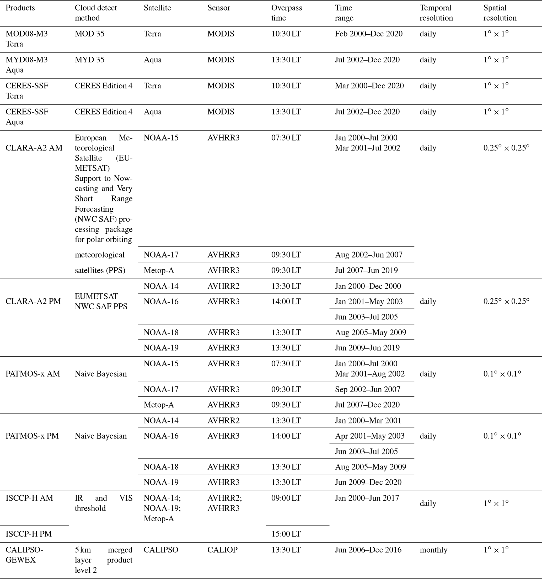
In view of the complementarity among the AVHRR-based, MODIS-based, and active sensor products, this study involved 10 passive-satellite-derived products from MODIS and AVHRR, with the time period spanning from 2000 to 2020 along with an active-satellite-derived product from CALIPSO, with the time period spanning from 2006 to 2016. The experimental period only included the sunlit months from April to September because of the darkness of the Arctic winter. All the data are briefly described in Table 1. Our study aimed to provide accurate and reliable measurements of cloud fraction during the daytime in the Arctic region. To achieve this objective, we utilized cloud fraction data labeled as “daytime” from multiple satellite datasets.

The AVHRR sensors are aboard sun-synchronous orbit satellites collecting data in the morning or afternoon (NOAA, Metop-A/B). The morning (afternoon) orbits cross the Equator on their descending (ascending) node at approximately 07:30 LT (13:30 LT) (local time). Starting with NOAA-17 and all Metop satellites, AVHRR data are available from a midmorning orbit with the Equator crossing time at approximately 09:30 LT. However, complications arose from changes in the equatorial crossing times of individual AVHRR sensors due to satellite drift (Heidinger et al., 2014; Karlsson et al., 2013). The AVHRR has a nominal spatial resolution of 1.1 km at the nadir point, facilitating full global coverage twice daily (daytime and nighttime), but the products this study employed provide global area coverage data with a nadir footprint size of 1.1 km × 4.4 km (Stengel et al., 2017). Cloud detection algorithms of these latest satellite data have improved greatly in polar regions. However, some data gaps exist as a result of AVHRR scan motor errors (e.g., the NOAA-15 orbits were excluded in 2000 and 2001) and limitations of observation conditions (e.g., CLARA-A2 could not cover the central Arctic Sea in September).

The MODIS sensor is aboard both the morning satellite Terra and the afternoon satellite Aqua, with overpass times at the Equator of approximately 10:30 and 13:30 LT, respectively. MODIS produces complete near-global coverage in less than 2 d. The 36 channels from the visible to the thermal infrared part of the spectrum provide abundant spectral information for cloud parameter retrieval. The new version datasets have improved the cloud detection algorithms in polar regions, whereas some researchers found overestimated CF in snow/ice surface in the new datasets when compared with active sensor data (Marchant et al., 2020, 2016; Paul, 2017; Trepte et al., 2019). Although some differences exist between Terra and Aqua, the consistency between these two satellites cannot be ignored (Trepte et al., 2019).

The CALIPSO satellite combines an active light detection and ranging (lidar) instrument (Cloud-Aerosol LIdar with Orthogonal Polarization – CALIOP lidar) with passive infrared (Imaging Infrared Radiometer) and visible imagers (Wide Field Camera) to probe the vertical structure and properties of thin clouds and aerosols worldwide (Winker et al., 2007; Vaughan et al., 2004; Hunt et al., 2009; Vaughan et al., 2009; Winker et al., 2009). As the most accurate currently active spaceborne instrument for detecting clouds, CALIPSO has a 16 d repeat cycle with equatorial overpass time at 13:30 LT. CAL_LID_L3_GEWEX_Cloud-Standard-V1-00 is a widely used gridded cloud product with a spatial resolution of an equal angle grid of 1^∘ × 1^∘ (Claudia et al., 2012).

Table 1 Satellite cloud fraction products used in this research.

2.2 Ground observation data

2.2.1 Climatic Research Unit gridded Time Series

The Climatic Research Unit gridded Time Series (CRU TS) is a widely used climate dataset covering all land surfaces except Antarctica, which uses angular distance weighting to interpolate monthly climate anomalies from extensive networks of weather station observations onto a 0.5^∘ grid (Harris et al., 2020, 2014). This dataset was first published in 2000, and the latest version, CRU TS4.05, contains 10 variables including cloud cover for the period 1901–2020 (Harris et al., 2020). The percentage of cloud cover was derived from observations of sunlit hours, and CRU TS4.05 output files are actual values not anomalies.

2.2.2 International Comprehensive Ocean-Atmosphere Data Set

The International Comprehensive Ocean-Atmosphere Data Set (ICOADS) is the most extensive freely available archive of global surface marine data, which has been assimilated into all major atmospheric, oceanic, and coupled reanalyses (Freeman et al., 2017). The ICOADS report is derived from synthetic observations by ships, buoys, coastal platforms, or oceanographic instruments. This dataset offers a gridded monthly summary for 2^∘ latitude × 2^∘ longitude boxes dating back to 1800 (and 1^∘ × 1^∘ boxes since 1960) (Woodruff et al., 2005). The available climatic variables include cloud cover and other atmospheric parameters (Bojinski et al., 2014). In this study, we used the 1^∘ × 1^∘ cloud cover data in sunlit months (April to September) spanning 2000 to 2020. In particular, we obtained the “fraction of observations in daylight” data from the ICOADS dataset, which allowed us to select only the data points corresponding to daytime observations. During our analysis, we imposed a threshold of 0.8 for the fraction of observations in daylight, ensuring that we only included the data with high confidence in our study.

2.3 Reanalysis data and model data

In recent decades, atmospheric reanalysis datasets have emerged as a valuable resource for studying climate processes and predictability, offering a long-term, gridded depiction of atmospheric conditions. These datasets rely on state-of-the-art data assimilation systems, which integrate observational data and underlying models to create a continuous record of historical weather patterns. Through the use of various atmospheric variables, they provide insight into past weather phenomena. The utilization of these datasets could prove imperative in conducting research within areas that are limited in data availability, such as the Arctic. Several studies have investigated the performance of reanalyses over the Arctic for a variety of fields including CF (Yeo et al., 2022; Kennedy et al., 2012; Huang et al., 2017). However, the systematic errors of climatological reanalysis CF are substantial for Arctic clouds because of the complexity of cloud microphysical processes and lack of good observation. In-depth comparisons, as conducted by Walsh et al. (2009), have identified difficulties in adequately depicting persistent low-level CF in summer via reanalysis models (Walsh et al., 2009).

ERA5 is an advanced atmospheric reanalysis product developed by the European Centre for Medium-Range Weather Forecasts (ECMWF). It provides information on cloud properties, including cloud fraction, cloud ice, cloud liquid, rain, and snow water content, which are estimated using the prognostic equations developed by Tiedtke in 1993 (Tiedtke, 1993). This method accounts for physical processes that act as sources or sinks of clouds, such as convection and condensation. In addition, the outdated diagnostic temperature-dependent approach for phase partitioning in mixed-phase clouds has been replaced with a more sophisticated, prognostic method developed by Forbes and Ahlgrimm in 2014 (Forbes and Ahlgrimm, 2014). The updated radiation scheme in ERA5 employs the Monte Carlo independent column approximation with generalized overlap for sub-grid cloud representation, enhancing the accuracy of the product.

This study uses the CF of “ERA5 hourly data on single levels from 1959 to present”, and the CF parameter has been regridded to a regular lat–long grid of 0.25^∘ and calculated by making assumptions about the degree of overlap/randomness between clouds at different heights.

The climate model is also a valuable tool for climate studying. However, comparisons of climate models with Arctic observations over the past 3 decades have revealed persistent challenges for simulating the Arctic climate, which is partially attributed to imprecise cloud fraction data (English et al., 2014). The sixth phase of the Coupled Model Intercomparison Project (CMIP6) has been used in many research papers about climate. Among them, the simulation data of the Meteorological Research Institute – Atmospheric General Circulation model version 3.2S (MRI-AGCM3-2-S) climate model provide a basis for climate research designed to answer fundamental scientific questions and serve as a resource for authors of the Sixth Assessment Report of the Intergovernmental Panel on Climate Change (IPCC-AR6). The model employed in this study is derived from the operational weather prediction model of the Japan Meteorological Agency (JMA). It integrates quasi-conservative semi-Lagrangian dynamics, a radiation scheme, and a land surface scheme that was initially designed for a climate model. Utilizing observed sea surface temperature (SST) as well as SST alterations forecasted by atmosphere–ocean coupled models, we carried out simulations of both present-day and future climate conditions. This model was released in 2017 and provided CF parameters at native nominal resolutions of 25 km. This resolution employed in the model is as fine as those employed by regional climate models (RCMs) in recent studies. Small-scale phenomena are realistically simulated in the high-resolution model while keeping the same quality of global-scale climate representation as the lower-resolution models.

The study involved a comparison of pre- and post-fusion CF data with reanalysis and model data. The aim was to underscore the significant role of fused data in improving the consistency of CF between satellite observations, reanalysis data, and model data.

3 Data preprocessing and methodology

In this study, we propose a fusion algorithm framework that combines data from multiple satellites to provide CF datasets with high spatiotemporal coverage and improved accuracy. Figure 1 shows a flowchart of the general process, which includes four parts. First, the original data were preprocessed before data fusion, a process that included data quality control and data resampling. Second, bias correction of passive sensor data was conducted using active data with the CDF matching method. Third, to comply with BME's stationarity prerequisite that assumes constancy of mean and variance, we removed the spatiotemporal trend of the original satellite CF data over the study area using the spatiotemporal moving-window filter method. Fourth, the spatiotemporal covariance function was modeled based on the isotropic residual data, and then the entropy was maximized with covariance constraint. All the satellite-based CF data were treated as soft data, so that the associated uncertainties were incorporated into the fusing process.

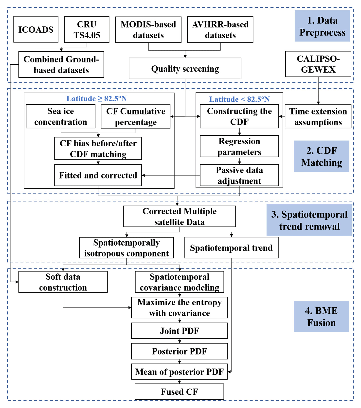
Figure 1 Flowchart for merging the multiple satellite cloud fraction products based on cumulative distribution function matching and the Bayesian maximum entropy method.

3.1 Data preprocessing

Over the Arctic, the cloud detection capabilities of passive sensors are always limited by spectral channels, while active sensors are not susceptible to these effects (Liu et al., 2010; Y. H. Liu et al., 2012b; Kotarba, 2020; Shupe et al., 2013). To obtain more accurate fused CF results, it is necessary to correct these passive sensor products using active sensor data before merging.

For satellite datasets, statistics always have the Scientific Data Set (SDS) name suffix “_Standard_Deviation” and which are computed by calculating an unweighted standard deviation of all pixels or samples within a given 1^∘ grid cell. The large CF standard deviations (SDs) of satellite datasets represent the large uncertainties of CF detection (Ackerman et al., 2008; Stengel et al., 2017). In this study, we calculated the relationship between differences in SDs and CFs of passive/active sensor datasets and found that the larger the standard deviation, the more serious the underestimation of passive sensors. For the products with standard deviation flags, including MOD08 Terra/Aqua, CLARA-A2 AM/PM, and the PATMOS-x AM/PM, we used the 90th percentile of the daily standard deviation as scene-based dynamic thresholds to screen CF data.

However, no standard deviation information was available for CERES-SSF Terra/Aqua and the ISCCP-H AM/PM datasets. Based on research that shows ignoring optically very thin clouds could increase the agreement between passive sensor data and the CALIPSO data, the 0.15 cloud optical thickness (COT) dataset was selected as the quality threshold in this study.

3.2 CDF matching

A widely used scaling strategy known as CDF matching can be used to adjust the distribution of the target dataset to the range of reference data under the constant relative relationship. Several studies have proved that the process of adjusting this distribution does not change the variation of original satellite-based products but rather aligns the value range with that of the reference data (Y. Y. Liu et al., 2011; Brocca et al., 2011; Xu and Cheng, 2021). Based on similar seasonal fluctuations of the passive sensor CFs and active sensor data, the time series of passive sensor data from each grid box in the Arctic region were adjusted to the values of the paired CALIPSO-GEWEX latitude and longitude grid. However, the CALIPSO-GEWEX data could not cover regions with a latitude greater than 82.5^∘ N, and the temporal range only covers 2006–2016. To correct the CF bias over the entire Arctic region, two strategies were considered.

First, for the regions with enough reference data, the CF data of all passive sensors were directly adjusted by CDF matching. The matching approach includes three steps: (1) constructing the cumulative distribution function, (2) deriving regression parameters, and (3) adjusting the original data with regression parameters. In our study, we use a 3-month moving mean to eliminate the uncertainties in CALIPSO-GEWEX data caused by the limitation of sampling quantities and frequencies. The filtered daily passive sensor datasets were resampled as monthly mean data, and then the CDFs were constructed for every dataset based on the same method used for the active data. A least-square fit was used to derive the relationship between the reference and the target datasets. Based on the analysis of Liu et al. (2022), the seasonal variation of CF for multiple satellites was greater than the interannual changes in CF (Liu et al., 2022). We propose an additional assumption that the CDF ratio between active and passive sensor data remains constant over the years in a 1^∘ × 1^∘ grid cell.

Second, it was difficult to implement the CDF matching strategy for areas beyond the coverage of active sensor data. Considering the relationship among the CF bias before and after CDF correction, the cumulative percentage of CF (CPCF, the average CF over an interval of SIC), and the sea ice concentration (SIC), a fitting function is proposed to correct the CF data.

After executing the abovementioned steps, we obtained the corrected multiple satellite data.

3.3 Spatiotemporal trend analysis and removal

The BME theory was constructed based on the hypothesis of spatiotemporal random field (S/TRF) (Nazelle et al., 2010; Christakos, 2000; He and Kolovos, 2017), which means that all the variables used for this process are homogeneous and isotropous. However, a natural process that evolves in space–time, such as the distribution of CF, can be divided into a heterogenetic global spatiotemporal trend and a spatiotemporally isotropous residual, following Eq. (1):

$$\begin{array}{}\text{(1)}& {\mathrm{CF}}_{\left(s,t\right)}={\stackrel{\mathrm{‾}}{\mathrm{CF}}}_{\left(s,t\right)}+{\mathrm{CF}}_{\mathrm{res}\left(s,t\right)},\end{array}$$

where (s,t) represents space and time, ${\stackrel{\mathrm{‾}}{\mathrm{CF}}}_{\left(s,t\right)}$ represents the global spatiotemporal trend, and CF_res(s,t) represents the stochastic anomalies of the variable. To meet the second-order stationarity assumption (constant mean and variance), it is necessary to remove the global spatiotemporal trend before estimating the spatiotemporally autocorrelated structure of the data (Spadavecchia and Williams, 2009; Tang et al., 2016). In this study, the global spatiotemporal trend was calculated using a spatiotemporal filter window with a size of 5^∘ (longitude) × 5^∘ (latitude) × 3 (months).

Figure 2 shows a histogram of the original combined satellite CF data, the global spatiotemporal trend, and the residual spatiotemporally isotropous component. From these distributions of the histogram, the residual is approximately normally distributed, which meets the requirement for modeling the structure of the spatiotemporal autocovariance.

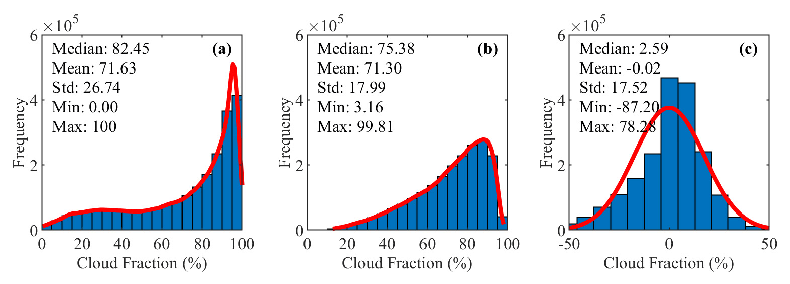
Figure 2 Histograms of (a) original combined satellite cloud fraction, (b) global spatiotemporal trend, and (c) spatiotemporally isotropous component, for the entire Arctic area (example using 2010 data).

3.4 BME fusion

3.4.1 Spatiotemporal covariance modeling

In spatiotemporal geostatistics, a covariance function indicates the spatial and temporal dependency of the data, which decreases as distance/time increases (Griffith, 1993). The spatiotemporal variation of the CF also can be expressed by a spatiotemporal covariance function. In the BME method, the experimental covariance can be calculated from point pairs at specific distances and then modeled by the commonly used covariance model (Cressie, 2015). This study uses a nested covariance model with two spatiotemporal exponential models to model the spatiotemporal covariance of the detrended combined CF data, following Eq. (2):

$$\begin{array}{}\text{(2)}& \begin{array}{rl}\mathrm{cov}(d,\mathit{\tau })& =c_{\mathrm{1}}\exp \left(-{\displaystyle \frac{\mathrm{3}d}{a_{s\mathrm{1}}}}\right)\exp \left(-{\displaystyle \frac{\mathrm{3}\mathit{\tau }}{a_{t\mathrm{1}}}}\right)\\ & +c_{\mathrm{2}}\exp \left(-{\displaystyle \frac{\mathrm{3}d}{a_{s\mathrm{2}}}}\right)\exp \left(-{\displaystyle \frac{\mathrm{3}\mathit{\tau }}{a_{t\mathrm{2}}}}\right),\end{array}\end{array}$$

where d is the spatial lag, and τ is the temporal lag between point pairs at coordinates p(s,t) and coordinates $p^{\prime }(s^{\prime },t^{\prime })$; c₁ and c₂ are the partial sill variances of the two exponential models; a_s1 and a_s2 are the spatial ranges of the two exponential models; and a_t1 and a_t2 are the temporal ranges of the two exponential models. When the S/TRF is characterized by spatial and temporal stationarity, it is only the relative distance between any couple of locations that affects the covariance function. Specifically then, the covariance function has the same value $cx(p,p^{\prime })=cx(r,t)$ for any location pair ($p,p^{\prime }$) separated by the same spatial distance vector $\mathit{r}=s^{\prime }-s$ and same temporal distance lag $\mathit{\tau }=t^{\prime }-t$ (Christakos and Serre, 2000). In this study, the parameters for spatiotemporal covariance are modeled separately for each year. The modeled results show that the model has a spatial range of 2^∘, a temporal range of 3 months, and a partial sill variance of 0.85 for local-scale CF (the first nested covariance model). And for the large range CF, the model has a spatial range of 30^∘, a temporal range of 6 months, and a partial sill variance of 0.15 (the second nested covariance model).

3.4.2 Construction of soft data

BME treated the informative content with uncertainty from different sources as soft data (He and Kolovos, 2017). For example, the observed data were accompanied by obvious sources of uncertainty such as inaccuracy in measuring devices, modeling uncertainties, and human error. In this study, the CF data of passive sensor products are viewed as soft data. For the BME method, a key conceptual aspect is that the framework does not impose any restrictive assumptions about the PDFs of soft data. Hence, a parameterized statistical distribution of different sources of information can be used to replace the real PDFs (Nazelle et al., 2010). Soft data could be probabilistic or interval soft data (Christakos, 2000). In this study, the differences between satellite data and ground observations followed normal distributions approximately. Therefore, the passive sensor data used for fusion were all treated as soft data with a Gaussian distribution, following Eq. (3):

$$\begin{array}{}\text{(3)}& {\mathrm{CF}}_{\mathrm{sate},x}={\mathrm{CF}}_{\mathrm{ground},x}+{\mathit{\epsilon }}_x,\end{array}$$

where CF_sate,x and CF_ground,x are the satellite CF data and the corresponding ground observations, respectively, and ε_x is an independent random error, following Eq. (4):

$$\begin{array}{}\text{(4)}& \mathit{\epsilon }\sim N\left({\mathit{\mu }}_{\mathit{\epsilon }},{\mathit{\sigma }}_{\mathit{\epsilon }}^{\mathrm{2}}\right),\end{array}$$

where μ_ε represents the mean of random error, and ${\mathit{\sigma }}_{\mathit{\epsilon }}^{\mathrm{2}}$ represents the variance (Tang et al., 2016).

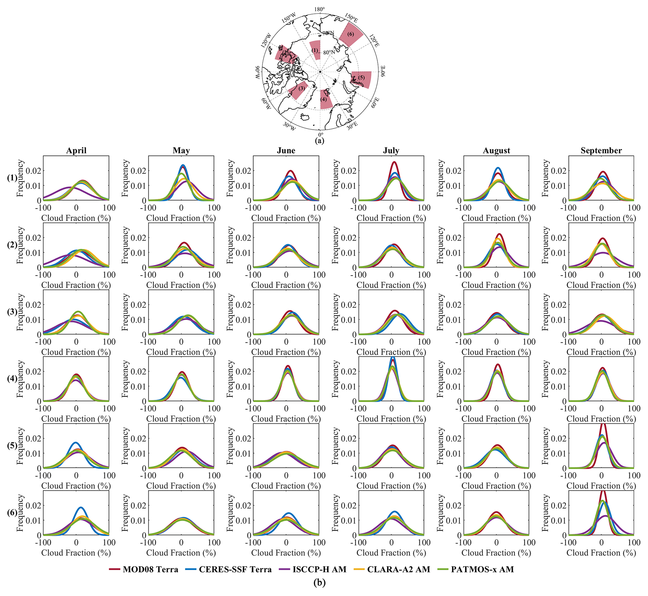
Figure 3 Gaussian probability density functions of the random errors between each type of satellite data and ground observations at six randomly selected regions of interest from April to September.

Because the uncertainties in each satellite CF data vary at different spatial and temporal scales, using the average uncertainty of the entire dataset to construct soft data over the entire study area will undoubtedly neglect the spatiotemporal variation of uncertainties. In this study, six regions were randomly selected to analyze the probability density functions (PDFs) of random errors (Fig. 3). Large inconsistencies were observed for the PDFs in land and ocean regions, and the temporal variation was also an important factor in inconsistencies. We constructed the soft data for CF data over land and ocean regions in every month separately. Considering the large errors in the Greenland Ice Sheet (GrIS), we calculated the PDF of random error separately for that region.

For each grid box, the CFs of different satellite data were converted into a Gaussian distribution probability soft data, individually (Tang et al., 2016). The soft data were expressed as

$$\begin{array}{}\text{(5)}& {\mathrm{CF}}_{\mathrm{soft},\mathrm{sate}}\sim N\left({\mathrm{CF}}_{\mathrm{sate}}+{\mathit{\mu }}_{\mathit{\epsilon }},{\mathit{\sigma }}_{\mathit{\epsilon }}^{\mathrm{2}}\right),\end{array}$$

where CF_sate is the detrended CF value of multiple satellite datasets; the mean and variance of the Gaussian distribution probability soft data were expressed by CF_sate+μ_ε and ${\mathit{\sigma }}_{\mathit{\epsilon }}^{\mathrm{2}}$, respectively.

3.4.3 Using the BME method for multiple CF data fusion

The BME method can be used to merge continuous variables of satellite data for some atmospheric parameters. To simplify the heterogeneity and anisotropic variability, the residuals were considered only in the fusion process. Assuming that various adjacent observations from satellites were available with irregular spatial and temporal gaps, the nonlinear mean estimation $\stackrel{\mathrm{‾}}{x_k}$ of CF at the location (s_x, s_y) at time t was estimated as

$$\begin{array}{}\text{(6)}& \stackrel{\mathrm{‾}}{x_k}=\int x_{k}f\left(\left.x_k\right|x_{\mathrm{soft},\mathrm{1}},x_{\mathrm{soft},\mathrm{2}}\mathrm{\dots }{x}_{\mathrm{soft},n}\right)\mathrm{d}{x}_k,\end{array}$$

where $f\left(x_k\right|x_{\mathrm{soft},\mathrm{1}},x_{\mathrm{soft},\mathrm{2}}\mathrm{\dots }{x}_{\mathrm{soft},n}$) is a posterior PDF over the spatiotemporal adjacent grid observations, and $x_{\mathrm{soft},\mathrm{1}},x_{\mathrm{soft},\mathrm{2}}\mathrm{\dots }{x}_{\mathrm{soft},n}$ are the probabilistic Gaussian soft data derived from multiple satellite data. The posterior PDF at the estimation point updates from the prior PDF in the Bayesian rule when soft data are involved, so the relationship can be expressed as

$$\begin{array}{}\text{(7)}& \begin{array}{rl}& f\left(x_k\mathrm{|}{x}_{\mathrm{soft},\mathrm{1}},x_{\mathrm{soft},\mathrm{2}}\mathrm{\dots }{x}_{\mathrm{soft},n}\right)\\ & ={\displaystyle \frac{f\left(x_{\mathrm{soft},\mathrm{1}},x_{\mathrm{soft},\mathrm{2}}\mathrm{\dots }{x}_{\mathrm{soft},n},x_k\right)}{f\left(x_{\mathrm{soft},\mathrm{1}},x_{\mathrm{soft},\mathrm{2}}\mathrm{\dots }{x}_{\mathrm{soft},n}\right)}},\end{array}\end{array}$$

where $f(x_{\mathrm{soft},\mathrm{1}},x_{\mathrm{soft},\mathrm{2}}\mathrm{\dots }{x}_{\mathrm{soft},n}$) represents the prior PDF of the spatiotemporally isotropous CF at the adjacent grid, and $f(x_{\mathrm{soft},\mathrm{1}},x_{\mathrm{soft},\mathrm{2}}\mathrm{\dots }{x}_{\mathrm{soft},n},x_k$) is the joint PDF without specific information. Generally, the joint PDF is represented by f_g(x_map), which can be calculated by maximizing the entropy under the constraint of the general knowledge g (Jaynes, 1957). When predicting the probability distribution of a random event, the larger the information entropy, the larger the amount of information obtained, and the result is closer to the actual situation under a most uniform probability distribution. In this study, general knowledge is the spatiotemporal covariance model, and to maximize the entropy, we introduce a Lagrange multiplier λ (Xia et al., 2022).

$$\begin{array}{}\text{(8)}& f_g\left(x_{\mathrm{map}}\right)={\displaystyle \frac{\exp \left(\sum _{\mathit{\alpha }=\mathrm{1}}^n{\mathit{\lambda }}_{\mathit{\alpha }}{g}_{\mathit{\alpha }}\left(x_{\mathrm{map}}\right)\right)}{\int \exp \left(\sum _{\mathit{\alpha }=\mathrm{1}}^n{\mathit{\lambda }}_{\mathit{\alpha }}{g}_{\mathit{\alpha }}\left(x_{\mathrm{map}}\right)\right)\mathrm{d}{x}_{\mathrm{map}}}}\end{array}$$

Finally, the expectation of spatiotemporally isotropous CF component can be calculated by solving these equations. Then the anisotropic spatiotemporal trend component of each grid was added to the expectation at the corresponding point to obtain the merged CF product.

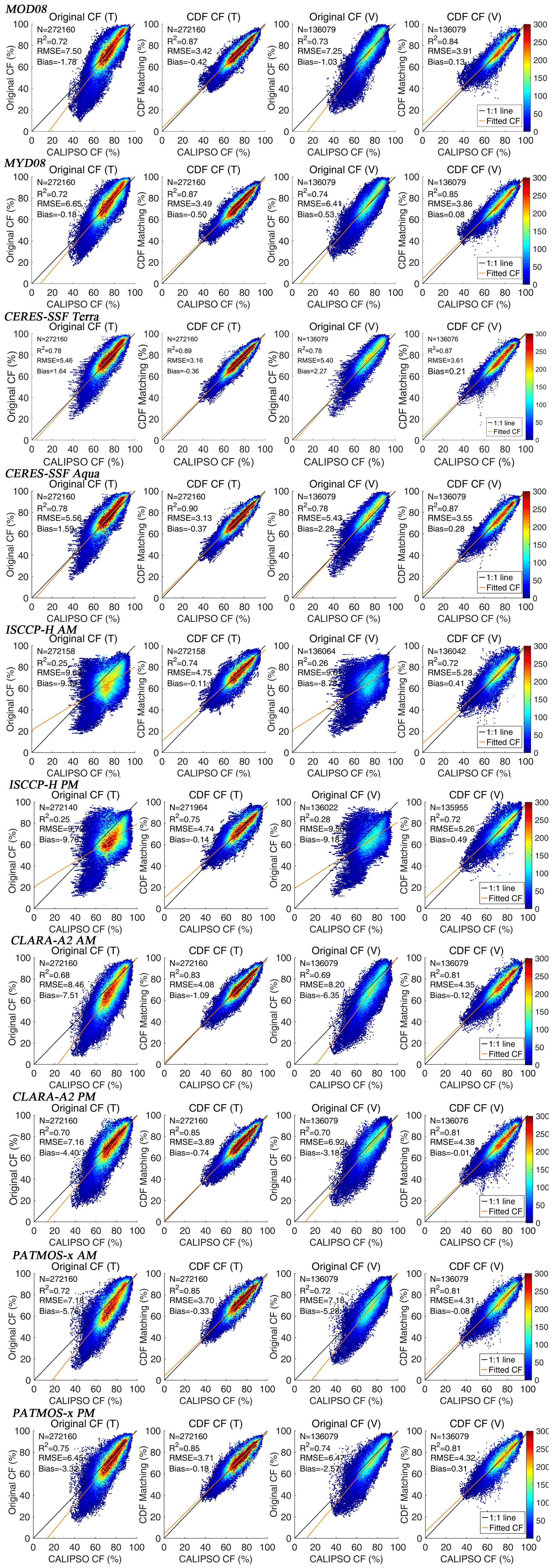
Figure 4 The scatter plots of the cloud fraction comparison between the passive and active sensor datasets at regions with latitudes less than 82.5^∘ N before and after cumulative distribution function matching: “(T)” means training data with time range from 2008 to 2014, and “(V)” means validation data from 2006, 2007, 2015, and 2016.

4 Results

4.1 Result of CDF matching

Figure 4 shows the scatter plots of the CF distribution before and after CDF matching from multiple passive and active sensors at the valid grid boxes with a latitude of less than 82.5^∘ N. Based on the assumption that the correction coefficient does not vary with time, the training datasets (T) were processed from 2008 to 2014, and the validation datasets (V) were processed in 2006, 2007, 2015, and 2016. In Fig. 4, “Original CF (T)” and “Original CF (V)” indicate the comparison of CALIPSO-GEWEX CF and that of the original passive sensor data, so that the “CDF CF (T)” and “CDF CF (V)” represent the comparison between CALIPSO-GEWEX CF and the corrected CF. In general, for all the passive sensor datasets, the CFs after CDF matching were closer to the 1:1 line than before CDF matching. R² increased by about 0.07–0.15, while that for the ISCCP-H products was over 0.45. The RMSEs decreased to one-third to one-half of what they were, and the biases decreased to approximately zero, which means that the CDF matching obviously corrected outliers and eliminated the average differences between the passive and active sensor CFs. From these scatter plots, we also understand that CDF matching plays an important role in low CFs (less than 60 %), which was always seen in April or on the GrIS (Liu et al., 2022).

In the sea ice regions, the relationships between CF bias of passive sensor data after and before CDF matching, CPCF, and SIC are shown in Fig. 5. The results indicated that the mean of the bias increased with the SIC. Moreover, the CPCF appeared to decrease with increasing SIC, and a negative correlation between CPCF and bias was also evident.

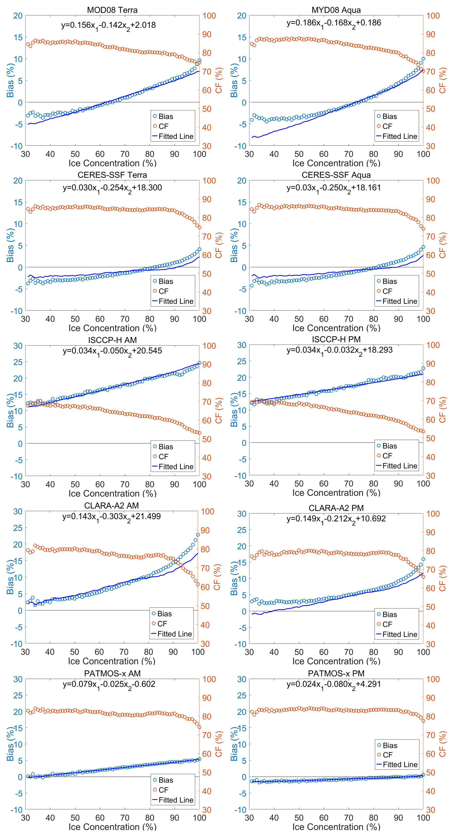
Figure 5 The relationship between cloud fraction bias of passive sensor data after and before cumulative distribution function matching, the cumulative percentage of cloud fraction, and the sea ice concentration in sea ice regions with latitudes less than 82.5^∘ N.

By virtue of this association, SIC and CPCF are modeled as dependent variables of the bias. Due to the predominant presence of sea ice over the domain located above 82.5^∘ N, we employ this functional association to remediate CF inaccuracies in the region, called “C-SIC Corrected” CF. The initial two columns of Fig. 6 depict a comparison between the CF of active data and passive data before and after correction by C-SIC in sea ice regions below 82.5^∘ N. The results indicate that R² of the corrected scatter plots increased slightly, but the RMSEs and bias were greatly reduced. In particular, the CF underestimated by passive sensors was similar to that of active sensors after correction. In our previous study, we have proven that this type of underestimation is very common (Liu et al., 2022). The third column of Fig. 6 shows the comparison of C-SIC Corrected CF and the CDF matching CF in sea ice regions with latitudes less than 82.5^∘ N. The results also showed that the C-SIC Corrected CFs have a high degree of consistency with the CFs corrected by the CDF matching, with R² over 0.75, RMSE less than 3.6, and bias less than 0.5. However, although the correction has improved the ISCCP-H CFs, they also showed large inconsistencies with the passive sensor data and the CDF matching data. Therefore, the ISCCP-H CFs in regions north of 82.5^∘ N were not included in the following fusion process.

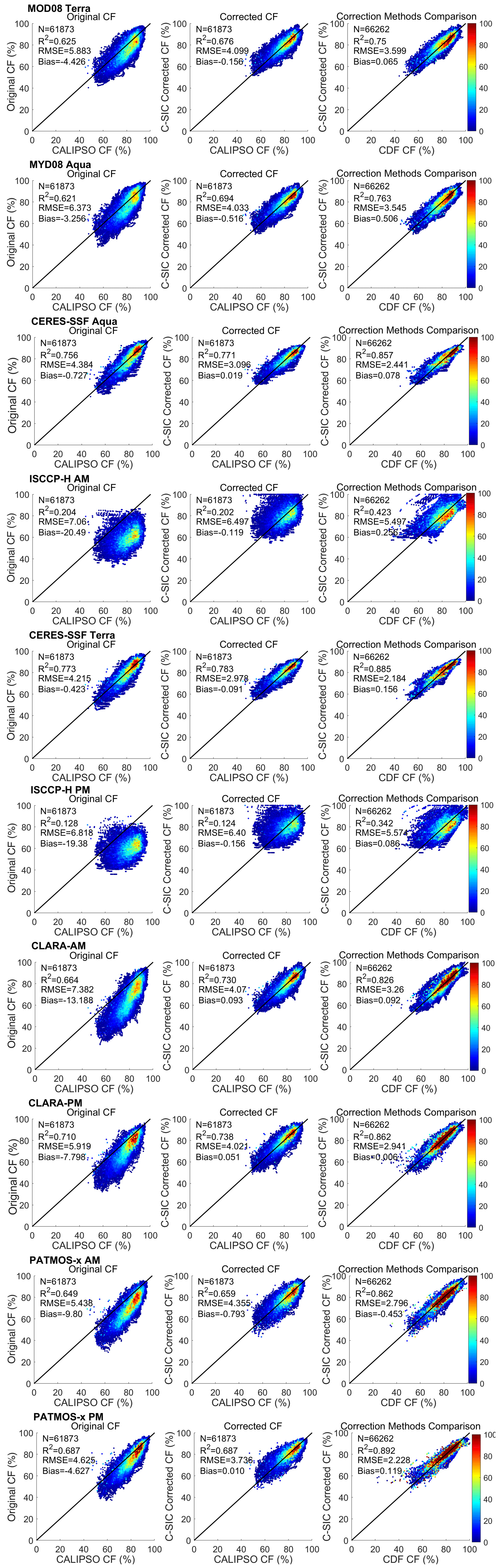
Figure 6 The scatter plots of the cloud fraction (CF) comparison between the passive sensor datasets and the active sensor datasets before (the first column) and after (the second column) using the method of CF corrected by the cumulative percentage of CF and SIC (C-SIC). And the scatter plots of the results comparison between C-SIC and cumulative distribution function matching (the third column).

Accompanying the decreases in the CF differences of the active and passive sensor data, the accuracy of individual passive sensor datasets for the entire Arctic during the experimental period was also generally improved. Moreover, the consistency of multiple satellite data has improved greatly. Figure 7 displays the standard deviation between 1^∘ × 1^∘ passive sensor CF data before and after the application of cumulative distribution function matching (latitude ≤ 82.5^∘ N) and C-SIC correction (latitude > 82.5^∘ N). The results obtained from different regions indicate an obvious decrease in the inconsistency between multiple passive sensor data after the correction with the aforementioned methods. In the Holarctic region, multiple passive sensor CFs saw a decrease in mean SD from 9.18 % to 5.75 %, with more than 50 % of the corrected data displaying a standard deviation within 5 %. The sea ice region saw the largest reduction rate of the mean SD, approximately 4.5 %. This reduction was mainly derived from an SD value range of 10 %–15 %, due to the limited detection capacity of passive sensor data in sea ice areas. Regions with latitudes less than 82.5^∘ N saw a decrease in mean SD of only 3.02 %. In contrast to the sea ice region, these land regions saw a smaller standard deviation between multiple satellite data. The distribution of SD frequency in regions over 82.5^∘ N and the entire sea ice area appeared similar, indicating that the C-SIC correction method was highly effective in the 82.5^∘ N regions. Although the relative values showed improvement, the absolute change appeared inconspicuous.

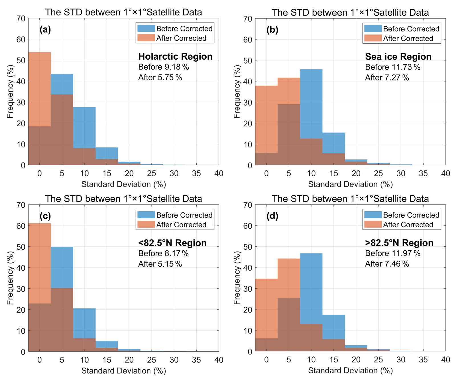
Figure 7 Standard deviation between 1^∘ × 1^∘ passive sensor cloud fraction before and after cumulative distribution function matching (latitude < 82.5^∘ N) and C-SIC Corrected (latitude > 82.5^∘ N).

4.2 Result of BME fusing

4.2.1 Spatial and temporal distribution of the fused CF

Figure 8 shows the spatial distribution of Arctic CF from the fused product, multiple satellite data, and ground observations. The results indicate that although most satellite-based products agreed relatively well with the ground-based observations in both the geographical distribution and the zonal average of Arctic CF at first glance, large disparities also appeared in some specific regions, whereas the fused product we proposed reduced these disparities apparently. For instance, nearly all the passive and active sensor products show the CFs over the GrIS were less than 60 %. However, CFs of ground-based observations over this region were reported as nearly 70 %, which is closer to that of the fused product. The sea regions of the central Arctic, which are covered by perennial sea ice/snow, are other areas where the passive sensor products always underestimate CF. From these figures, some passive sensor products, especially for the AVHRR-based datasets, have CFs that are about 10 %–20 % lower than those of active sensor data and ground-based observations. However, the fused CF has a similar magnitude to these two referred datasets.

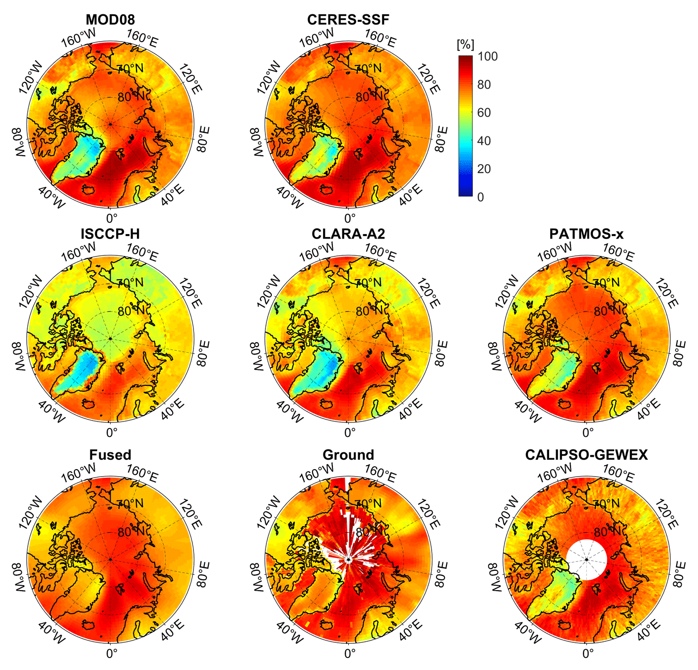
Figure 8 Distribution of the average cloud fraction of different datasets over the Arctic from 2000 to 2020. The time ranges for ISCCP-H and CALIPSO-GEWEX were from 2000 to 2017 and from 2006 to 2016, respectively.

By contrast, the ground-based CF products have a large data gap, because ground weather stations are sparsely distributed in the Arctic, so the limitation of sampling quantities and frequencies had the effect of limiting the spatial and temporal ranges of active sensor data. Moreover, the AVHRR-based products often suffer from missing data as a result of satellite failures or band switching (Hollmann, 2018); in addition, some passive sensor products such as CLARA-A2 have some spatial gaps over the Arctic Sea during autumn (Karlsson et al., 2017). Although we have eliminated a large number of low-precision daily data in preprocessing, the completeness of the merged multiple-satellite CF products is obviously higher than those of the original satellite-based data and ground-based observations in both spatiality and temporality, especially in regions of the Arctic Ocean. The spatial completeness (the ratio of available data to the CF grids of the entire Arctic) of the fused CF product was nearly 100 %, which is much larger than 54.09 % of ground-based products and 73.15 % of the active sensor product. Therefore, the fusion algorithm proposed by this study can not only obviously reduce the inconsistencies of Arctic CF between multiple satellite products and reference datasets but also effectively compensate for the data gaps caused by the lack of reference data.

It is well known that the CF in the Arctic regions fluctuates apparently with the change in seasons. To show the temporal accuracy of the fusion products, we analyzed the long time-series area-weighted mean of the CF. Figure 9 depicts the fluctuation of the mean value on a monthly basis for all data during sunshine periods (April to September) before and after fusion, as demonstrated by the time series. It is clear that the CF peaks in September and reaches a minimum in April. However, only the fused product always maintains a high level of consistency with the reference data, with the monthly mean CF varying from 62 % to 79 %. The overall area-weighted means of the differences between fused CF and CALIPSO-GEWEX CF and between fused CF and ground-based CF were about 0.91 % and 0.40 %, respectively, which are about one-third of the differences for MODIS-based products and reference products and about one-fifth to one-twentieth of the differences for AVHRR-based products and reference products. In land and ocean areas, the fusion algorithm clearly corrects the outliers with large deviations, such as the CF from CLARA-A2, PATMOS-x products, and the CERES-SSF products. The first two datasets are well-known for underestimating the Arctic CF dramatically (Karlsson et al., 2017; Karlsson and Dybbroe, 2010). In this study, the underestimation mainly occurred in April, with approximately 8 % and 3 % for those two datasets, respectively. The latter has often been reported to overestimate CF (Doelling et al., 2016; Trepte et al., 2019), and in this study the CERES-SSF products nearly overmeasure CF all year long from April to September. However, the fusion framework proposed by this study scales these underestimated values or overestimated values to a range similar to that of active sensor data by CDF matching; meanwhile, it takes into account the deviation from ground observations in the BME fusion process. The fused CFs can not only reduce the overestimation of CF by MODIS-based products but also decrease the underestimation of CF for AVHRR-based products, which obviously improves the consistency of CF between the active sensor, passive sensor, and ground-based observation dataset compared with the original data.

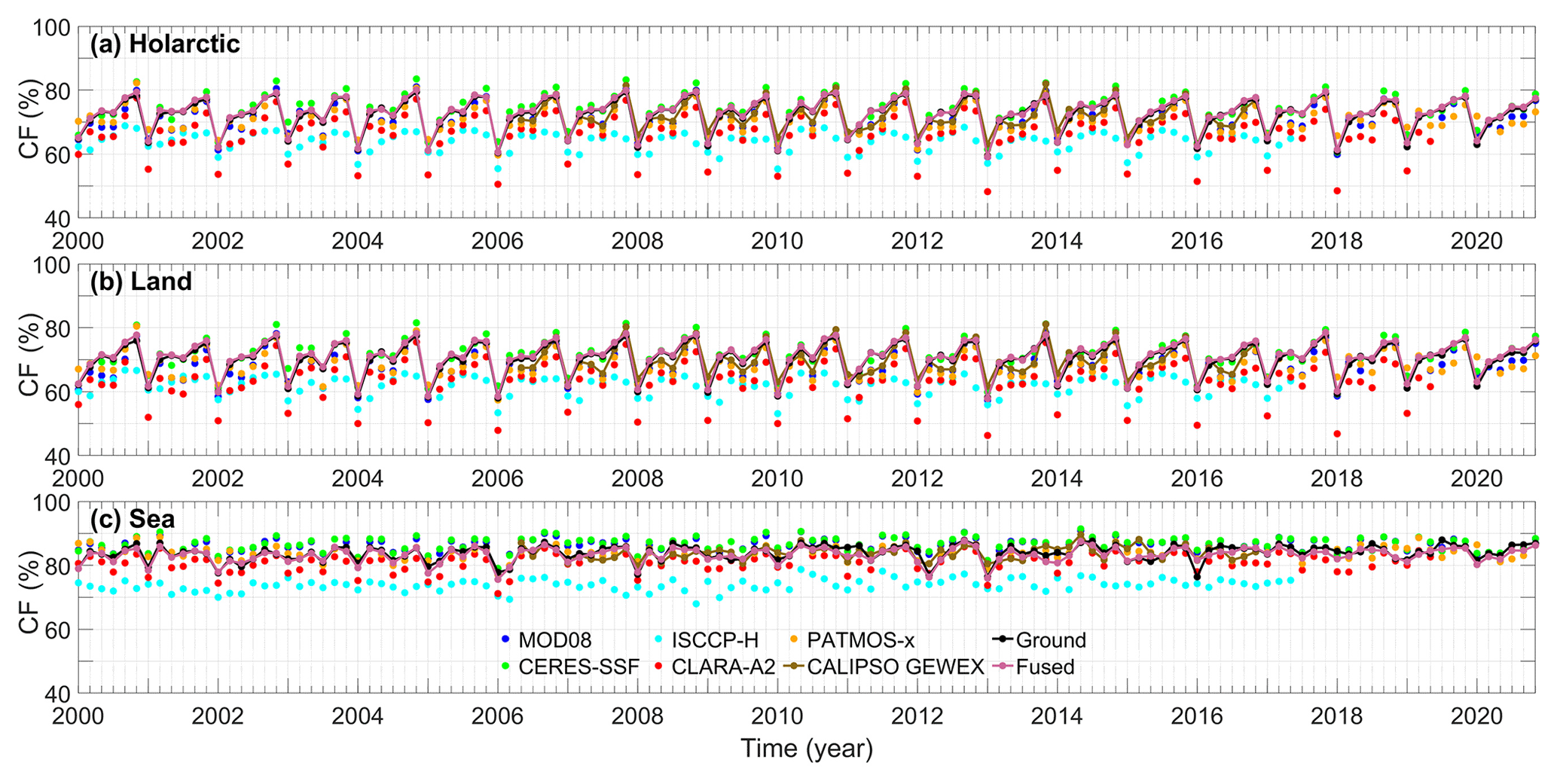
Figure 9 The area-weighted means of cloud fraction over (a) Holarctic, (b) land, and (c) sea regions for different products in the Arctic from April to September during 2000 to 2020. The time ranges for ISCCP-H and CALIPSO-GEWEX were from 2000 to 2017 and from 2006 to 2016, respectively.

4.2.2 Quantitative assessment of fused CF

To validate the fused CF and compare the accuracy of the fused results to that of several original satellite CFs, all the passive sensor CF products and the merged CF product were spatiotemporally compared with the CRU TS4.05 in land regions and ICOADS measurements in sea regions. The correlation coefficient (R²), root-mean-square error (RMSE), and mean bias (bias) were used to quantitatively evaluate the accuracies of the original and merged CF products. As Fig. 10 indicates, the scatter points of the fused CF product and ground-based observations were closer to the 1:1 line than that of the original satellite data. In this case, the fused data had the largest R² (0.51), lowest RMSE (6.95 %), and the lowest bias (0.35 %) for land regions. In addition, the fused data had the largest R² (0.42), the lowest RMSE (5.62 %), and the lowest bias (0.55 %) for sea regions.

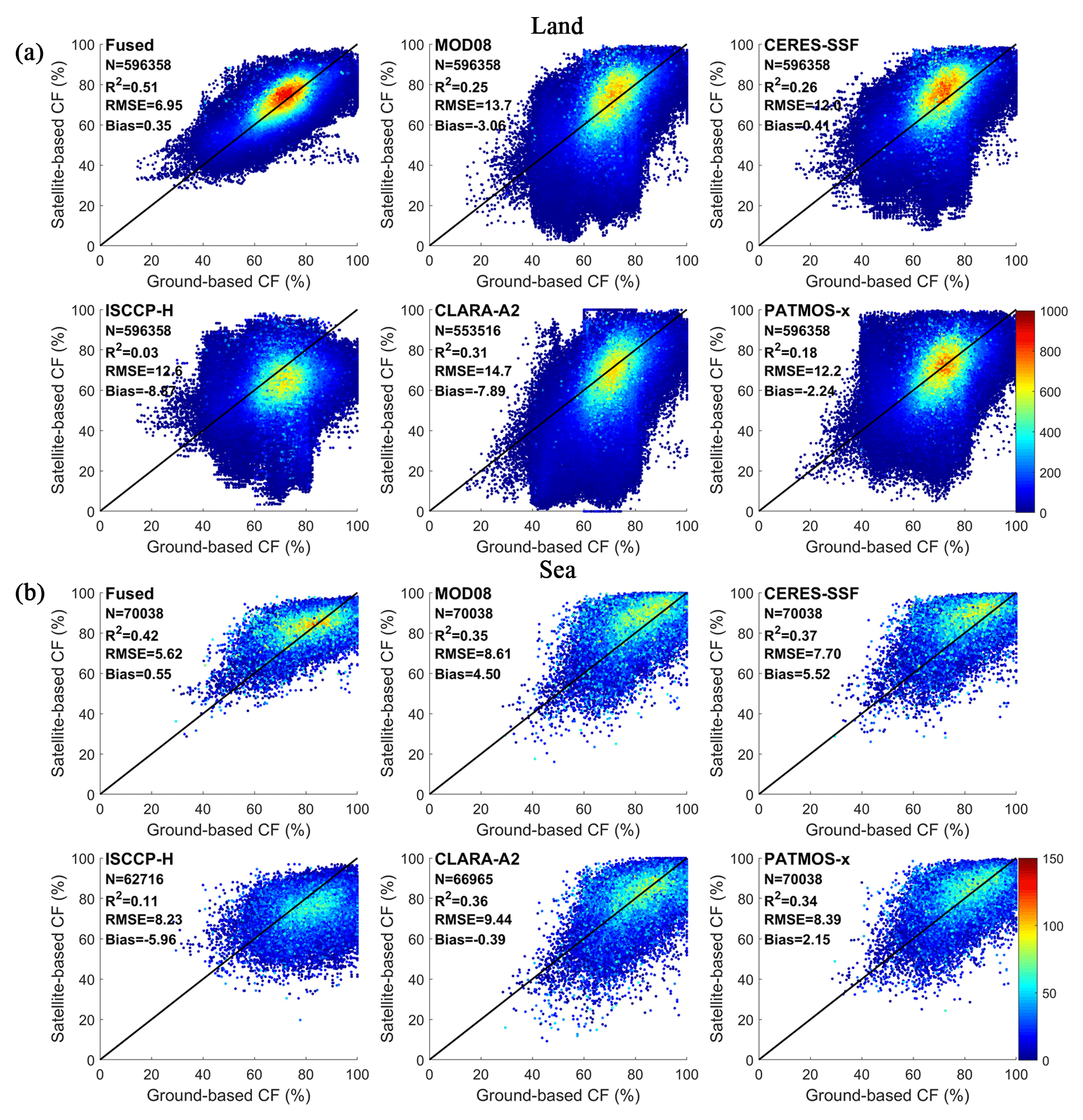
Figure 10 Validation of the fused cloud fraction and the original passive sensor datasets against the (a) CRU TS4.05 and (b) ICOADS datasets.

For land, it can also be seen that the fusion results have a strong ability to correct the satellite CF that is less than 30 %. These values were mainly found on the GrIS, in the Canadian islands, and on the central Eurasian continent. In addition, the RMSE of CF after fusion was only one-half of the original satellite data, which means that the overall distribution of the fused CF is better fitted to the reference data, and most of the CFs with differences over 30 % were corrected well.

The observations of ICOADS come from multiple observation platforms, and most of these platforms operate in open waters. The open-water regions varied mostly with the growth and decline of the SIC, which brings great spatiotemporal heterogeneity for the sampling of ICOADS. Therefore, in the verification process, the first step was to spatiotemporally collocate the satellite data with the ocean site. Figure 10b shows that R² of the fused CF only improved by about 0.05–0.08 when compared with most satellite data. However, the fusion algorithm reduces the RMSEs and bias obviously. The RMSEs of the fusion CF were about one-fourth to one-third of the original MODIS-based products and one-third to three-fifths of the original AVHRR-based products. The reductions of bias were about 4 %–5 % for MODIS-based products and about 2 %–5.4 % for AVHRR-based products.

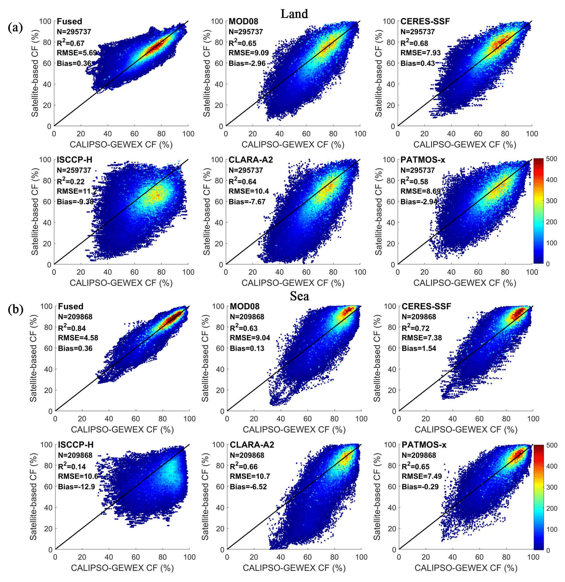
Figure 11 Validation of the fused cloud fraction and the original passive sensor datasets against the CALIPSO-GEWEX dataset over (a) land and (b) sea regions, with a temporal range from 2006 to 2016.

As the accepted reference for passive sensor products, CALIPSO-based products are considered to provide excellent data and are always used to validate the accuracy of cloud datasets. In Fig. 11, we compare the CFs of passive sensor products before and after fusion with those of the CALIPSO-GEWEX product. The results show that when compared with the original satellite data, the consistencies between the fused product and the active sensor product were further improved in both land and sea regions. The RMSEs were reduced to about one-third to one-half of the original values or approximately 5.69 % and 4.58 % for land and sea regions, respectively. Actually, the consistency of CFs between passive and active sensor datasets was higher than that between satellite data and ground observations. Except for the ISCCP-H products, the R² of original satellite data was over 0.63; that of fused CF only improved obviously in sea regions (about 0.12–0.21), while it improved slightly but in inconspicuously in land regions (about −0.01–0.1). This can be explained by the fact that the fusion algorithm greatly improves the low-value CFs in the land areas (especially on the GrIS) to levels similar to that of ground-based observations, while the CF of the active sensor data was no more than 60 %. Therefore, some overestimations for the fused CF existed when compared with the CALIPSO-GEWEX CF data. From the bias of Fig. 11a, we also see that the fusion algorithm can obviously improve the CF underestimated by the original satellite data. However, in the sea regions, the MODIS-based datasets seem to over-identify CF, especially when the CF was over 80 %. Meanwhile, the AVHRR-based datasets show underestimation when CF was less than 80 %. Obviously, the fused product corrected these CFs to a more suitable range.

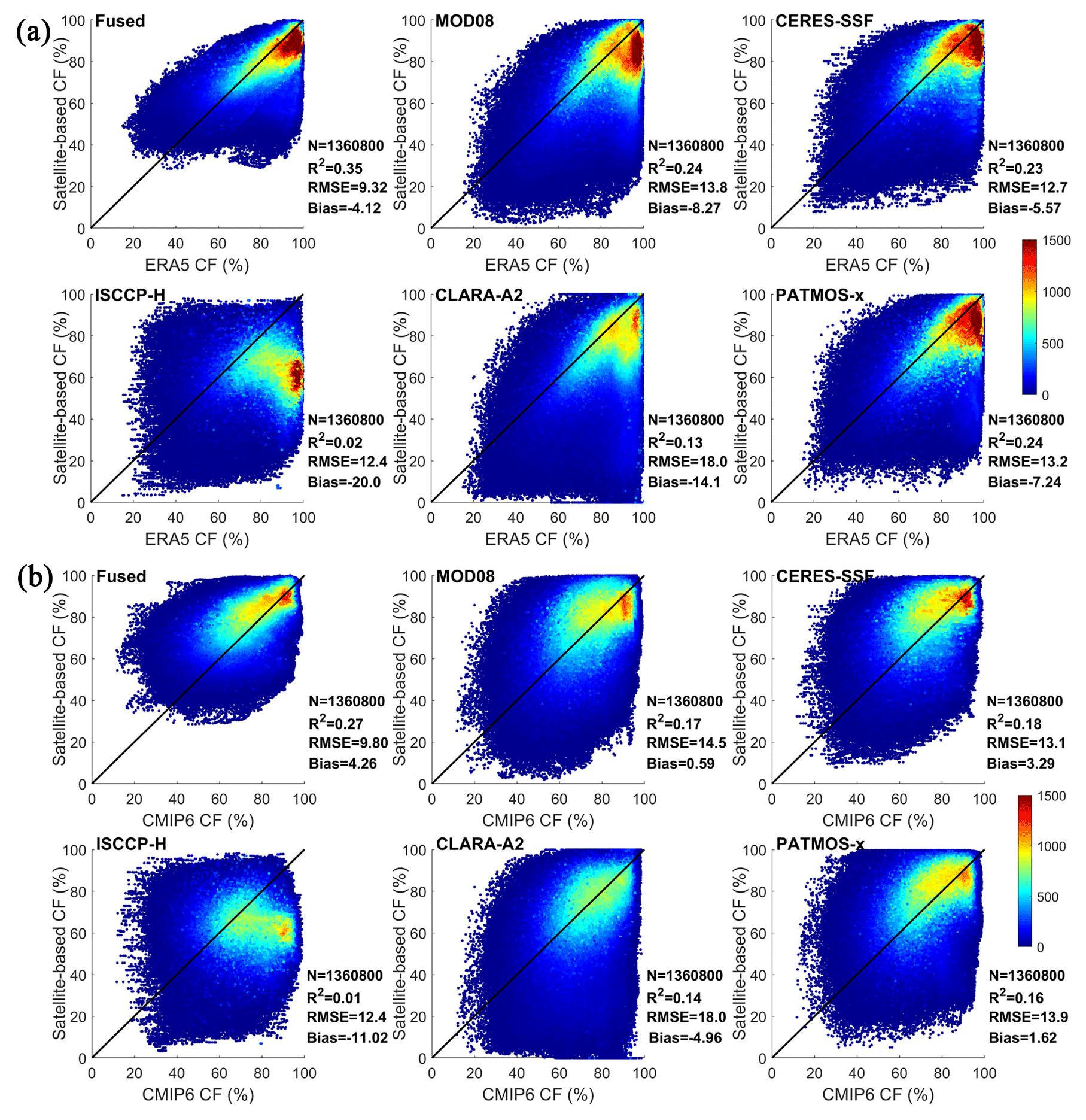
Figure 12 Validation of the fused cloud fraction (CF) and the original passive sensor datasets against (a) ERA5 CF dataset and (b) CMIP6 CF dataset over the Holarctic.

Reanalysis data and the climate model data are commonly used to provide a consistent and continuous dataset for long-term climate trends and variability studies. These datasets can provide insights into the behavior of the climate system that would be difficult to obtain from direct observations alone. To further show the advantages of the fusion results, we analyzed the difference in CFs between different satellite data, ERA5 reanalysis datasets, and the MRI-AGCM3-2-S climate model. As can be seen from Fig. 12, the fusion product greatly reduced the deviation in CF between the satellite data and the reanalysis dataset and the model data. When compared with the ERA5 CF dataset, the scatter points of fused CFs were more concentrated around the 1:1 line than those of the original satellite data. R² of the fusion product was about 1.5 times higher (improved about 0.18) than that of the original data, and the RMSEs and bias decreased to one-third of their original values (decreases of about 3.08 %–8.68 % and 1.45 %–15.88 %, respectively). This means that the distributions of the CFs over the entire Arctic of the fusion product were more consistent with those of the reanalysis CF dataset than the original satellite. However, the low absolute values also indicated that there were inescapable inconsistencies in some grids. The ERA5 dataset has usually been reported to overestimate CF in some regions of the Arctic, especially in the ocean regions (Yeo et al., 2022). In these regions the fused CF has slightly higher values than that of the ERA5 data.

The comparison results with the MRI-AGCM3-2-S CF show that, when compared with the original satellite data, the fusion method reduced the CF underestimation partly; these underestimations were often seen in April or over the central and western GrIS. In addition, R² was improved by about 0.14, and the RMSEs were reduced to one-fourth of their values of original satellite data (about 2.60 %–8.20 % reduction). However, although the fusion data relieve some CF overestimations that occurred in original passive sensor datasets, the scatter plot in Fig. 12 shows that the fusion CFs in some grids were significantly higher than the CF of model data (with bias by 4.26 %). These grids are usually found in the open-water areas of the Arctic Ocean, central Alaska, central Eurasia, and along the eastern margin of Greenland. Several studies have shown that the climate models underestimate the CF over these regions (Vignesh et al., 2020).

5 Discussion

5.1 The efficacy of CDF matching in CF fusion

The CDF matching approach was operated based on a time series CF considering the time-varying process of CF products at a specific longitude–latitude grid box. Compared with the metrics for the traditional approach, the CF of multiple passive sensor products was scaled to a level similar to the active sensor CF after CDF matching, so that the inconsistencies among multiple passive sensor CF datasets were reduced. To further evaluate the efficacy of CDF matching in the CF fusion process, we quantitatively evaluated the deviation between satellite data before and after CDF correction with ground-based observation data.

By comparing Figs. 10 and 13, we can infer that CDF matching can obviously improve the low value of CFs typical of satellite data, making such data more similar to those observed by ground-based sites. These improvements were more obvious for CFs over land regions. Among them, the largest bias correction was seen for the ISCCP-H products (about 7.9 % improvement) and the CLARA-A2 products (about 6.5 % improvement); the former always underestimated CF in the Arctic (Kotarba, 2015; Liu et al., 2022), and the latter have often been reported to under-identify CF over northern Canada, northern Russia, and across the entire GrIS in land regions and over the entire Arctic Ocean in April (Karlsson and Dybbroe, 2010). Note that the bias of CERES-SSF changes from 0.4 % to −0.72 % after CDF matching, because CERES-SSF products are usually reported to overestimate CF, and these overestimations were corrected reasonably. For the ocean regions, the ground references used in this paper were derived from multiple platform observations, which have great spatiotemporal heterogeneity. Therefore, a large CF discrepancy existed between satellite data and ocean observations. Almost all the passive sensor data have RMSEs and bias that would decrease after CDF correction by about 0.8 %–1.7 % and 0.68 %–5.26 %, respectively. The CDF matching mainly improves the CF in the high-value grid boxes of MODIS-based data and PATMOS-x data as well as in the CF in low-value grid boxes of ISCCP-H and CLARA-A2. Satellite observation covering open-sea areas typically presents a higher CF compared to station observation. Consequently, partial overestimation may persist despite correction by the CDF matching approach. In the subsequent fusion process, the difference between satellite CF and ground CF was taken into account, which can play a certain role in overfitting correction.

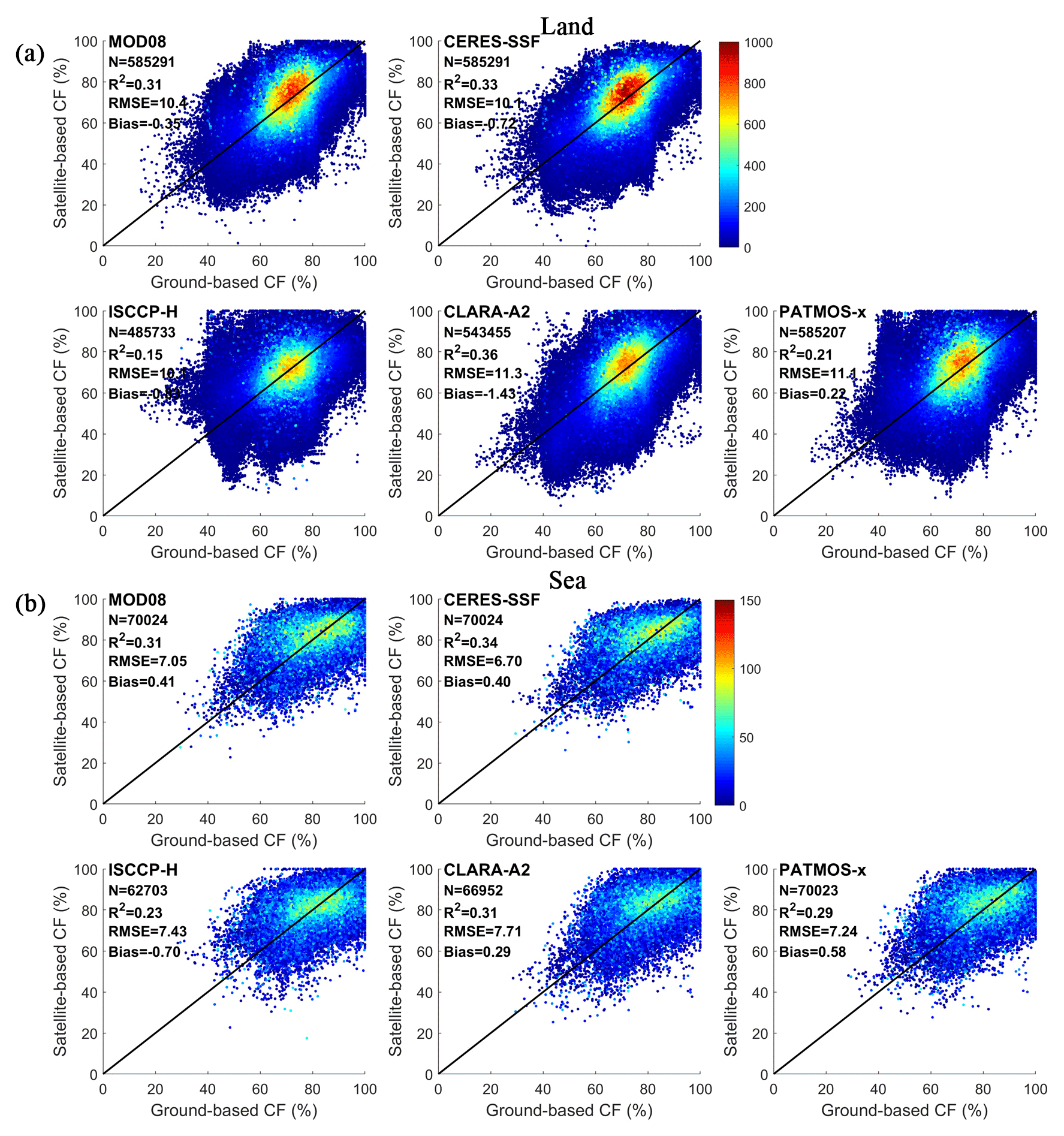
Figure 13 Validation of the corrected cloud fraction of passive sensor datasets after cumulative distribution function matching against (a) the CRU TS4.05 dataset over land regions and against (b) the ICOADS dataset over sea regions.

In addition, in the land area, CDF matching was directly carried out grid by grid. However, the short temporal range (2006–2016) of the reference data limits the production of long-time-series CF products. In this study, we proposed a hypothesis that the matching parameter in a specific grid box does not change with time. To prove the validity of this hypothesis, we conducted a sensitivity analysis on the matching parameters from the 5th to the 11th year at 1-year intervals. The findings indicate that any deviations in matching parameters were under 0.05 % when the time horizon exceeded 8 years. This demonstrates a level of stability in the correction coefficient when utilizing data for a period exceeding 11 years (Fig. A1). Figure 14 displays the variation in differences between satellite data and ground observations before and after conducting CDF matching throughout the duration of the study. These differences are calculated by subtracting the deviation between satellite data and ground observations subsequent to CDF matching from that prior to CDF matching. Clearly, the differences remained steady with time, and the maximum average annual difference was no more than 1.56 %, while part of it was derived from the orbit drift of satellite and variations in the spectral channel.

Figure 14 The difference in results between satellite data and ground observations before and after cumulative distribution function matching over the Arctic from 2000 to 2020.

5.2 The uncertainties of the original satellite data

CF products from different sensors have different degrees of uncertainty. As a knowledge-centered approach, the Bayesian maximum entropy approach could integrate informative content with uncertainty from different sources based on a rigorous theoretical support of considerable generality to achieve improved prediction accuracy. For example, the observed data that were accompanied by obvious sources of uncertainty such as inaccuracy in measuring devices, modeling uncertainties, and human error were treated as soft data in the BME strategy. For the CF datasets of multiple satellite, the uncertainties come from calibration error, orbit drift, signal degradation, and the errors of cloud detection algorithms (Liu et al., 2022). To achieve optimum estimation of CFs by combining data from multiple sensors, it is imperative to explicitly consider the uncertainties associated with the CF data that are being merged. In our study, the CF data of passive sensor products are viewed as soft data, and the uncertainty associated with different error sources can be expressed explicitly by probability distributions. Specifically, the soft data of multiple satellite CF datasets were constructed by comparing the spatiotemporally collocated satellite CFs and the ground-based records from CRU TS4.05 over land and from ICOADS over sea. Traditionally, the deviations between each satellite dataset and ground site observations at different times and different regions have been averaged to the entire datasets and then used to calculate the average uncertainty of these data. In this way, the spatial variation of uncertainty in each satellite dataset was ignored. Because the conditions that cause uncertainty are variable in time and space, the uncertainties in each satellite dataset were definitely not the same everywhere (Tang et al., 2016). This is especially true for the ICOADS data, which come from different platforms and introduce large inconsistencies in results. In this study, we constructed soft data for CF over land, ocean, and GrIS regions every month separately by analyzing the PDF differences for different regions and different months, which realized more consistent results with the ground observations. However, despite concerted efforts, determining the uncertainty for each grid remains challenging in light of the substantial temporal and spatial gaps of the reference data, particularly that which pertains to the marine domain.

5.3 The uncertainties of the fusion CF

To assess the fusion algorithm's reliability, we used the standard deviation of error within each grid value in the fusion process to quantify the uncertainties. Specifically, we determined the standard deviation of the predicted posterior probability density function on each grid point. Our findings demonstrate that, with the exception of the northern region of Greenland and part of the margin error, the standard deviation of error in other areas was within 3 % (Fig. 15). We attribute these discrepancies primarily to the underestimation of satellite observations, particularly the ISCCP-H data, by around 10 %–30 % in the central zone of Greenland. Moreover, the CF of ISCCP-H was significantly overestimated beyond the Greenland margin. Such significant inconsistencies can adversely affect the fusion results. In addition, because the CF of satellite data, particularly satellite data based on AVHRR, was significantly lower than that of ground-based observation data and active sensor data in April and because a significant difference existed between different datasets, the standard deviation of error after fusion marginally increased in April, with some areas at approximately 4 %. It should be noted that our fused data show an overestimation in the Greenland region. This is mainly because the fusion process prioritizes consistency between the fused data and ground observations. In specific applications, users can make corresponding adjustments based on active sensor data for calibration purposes.

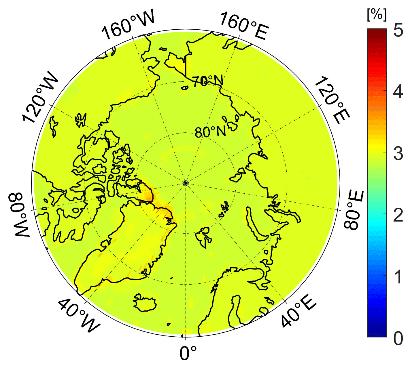
Figure 15 The mean error standard deviation of the fusion results.

6 Data availability

The fused CF product is available on the Zenodo repository at https://doi.org/10.5281/zenodo.7624605 (Liu and He, 2022). The gridded CF data are provided both in *.mat format (Fused_CF_ Arctic_ MAT, with a file size 9.91 MB) and in netCDF format (Fused_CF_Arctic_netCDF, with a file size 10.7 MB) at 1^∘ spatial resolution and monthly temporal resolution during 2000–2020 in percentages. The results in these two folders are exactly the same; users can download either format as needed.

7 Conclusions

The spatiotemporal inconsistency in existing satellite CF products would inhibit their application in climatological and energy budget studies. Over the Arctic region, the special climatic conditions and underlying surface characteristics limit the cloud detection abilities of passive/optical satellite sensors. The complementary features of the CF products derived from multiple satellite sensors in spatial completeness and accuracy make it possible to produce an improved CF product by merging data from multi-sensor satellite CF products.

In this paper, we propose a data fusion strategy for producing high-quality monthly CF data over the entire Arctic with a latitude higher than 60^∘ N during sunlit months from 2000 to 2020. Four key steps were involved in the proposed strategy: (1) data quality control, (2) correcting the bias of passive sensor data using CDF matching; (3) obtaining the spatiotemporally isotropous component by removing the spatiotemporal trends, and (4) producing very accurate CF data by fusing multiple satellite products and considering the uncertainty between satellite data and ground observations with the BME approach.

The fusion algorithm proposed by this study apparently reduced inconsistencies in the Arctic CF data acquired by multiple satellite products and the reference products spatiotemporally, resulting in 10 %–20 % reductions in CF differences between fused satellite products and the reference data, and an obvious improvement was seen across the GrIS and in the central Arctic Ocean. The results from 21-year datasets in the study areas demonstrate that the monthly mean CF of the fusion product varied from 62 % (April) to 79 % (September) during the study period, which is similar to that of the two reference datasets. After CDF matching, the inconsistencies of multiple satellite CF products were reduced by about 3.43 % for the entire Arctic, with a larger reduction (4.46 %) for sea ice regions. The overestimation of MODIS-based products and the underestimation of AVHRR-based products have been effectively corrected, with the CERES-SSF bias changing from 0.4 % to −0.72 % and the bias of ISCCP-H and CLARA-A2 decreasing by about 7.9 % and 6.5 %, respectively. After BME fusing, comparisons with the ground-based observations (CRU TS4.05 in land and ICOADS in marine areas) and the active sensor data CALIPSO-GEWEX show that R² improved by about 0.05–0.48 for different products; meanwhile, the overall RMSEs and bias of the fusion product were reduced by about 2.08 %–7.75 % and 1.6 %–12.54 %, with reductions of nearly 50 % and 67 % when compared with that of the original passive sensor data, respectively. When compared with the reanalysis CF dataset ERA5 and the model dataset MRI-AGCM3-2-S, R² increased by about 0.18 and 0.14, and RMSE and bias for reanalysis data decreased by about one-third of that for the original data, with reductions of about 3.08 %–8.68 % and 1.45 %–15.88 % for different data, respectively. The RMSEs for model data dropped to one-fourth of their original values (about a 2.60 %–8.20 % reduction). These metrics mean that the proposed fusion algorithm effectively removed CF data with differences greater than 30 % and made the fused Arctic CF estimation more robust than those data from a single satellite. Nevertheless, the fused product could completely cover the entire Arctic, especially the ocean regions, where the active sensor data and the ground-based data have large data gaps. Temporally, the fused data can complement the missing data caused by the faults of satellites carrying AVHRR sensors and the absence of Aqua data before 2002 as well as the temporal limitation of passive sensors.

In general, the proposed fusion algorithm combines the complementary features of multiple satellite CF datasets; it not only takes full advantage of the spatiotemporal autocorrelation among neighboring grids but also incorporates uncertainty estimates of multi-sensor CFs, such as the uncertainties of each passive sensor dataset, the uncertainties between passive and active sensor datasets, and the uncertainties between satellite data and ground-based observations. Through temporal and spatial expansion schemes, this fusion framework makes up for the disadvantages in spatiotemporal ranges of reference data. Finally, the fusion algorithm can generate a monthly 1^∘ × 1^∘ CF product covering the entire Arctic region during 2000 to 2020, which has positive significance for reducing the uncertainties of assessment of surface radiation flux and improving the accuracy of research related to climate change and energy budgets both regionally and globally. However, some overestimations were observed, especially in ocean regions. This may be attributed to the fact that the ocean stations are too sparse to play a certain role in correcting the overfitting of CDF. Although ICOADS is a widely used ocean validation dataset, it has great spatiotemporal heterogeneity as it comes from a variety of different observation platforms, and the sampling is affected by the extent of sea ice. Better reference data should be explored to further improve the uncertainty involved in the assessment of the fused product.

Appendix A

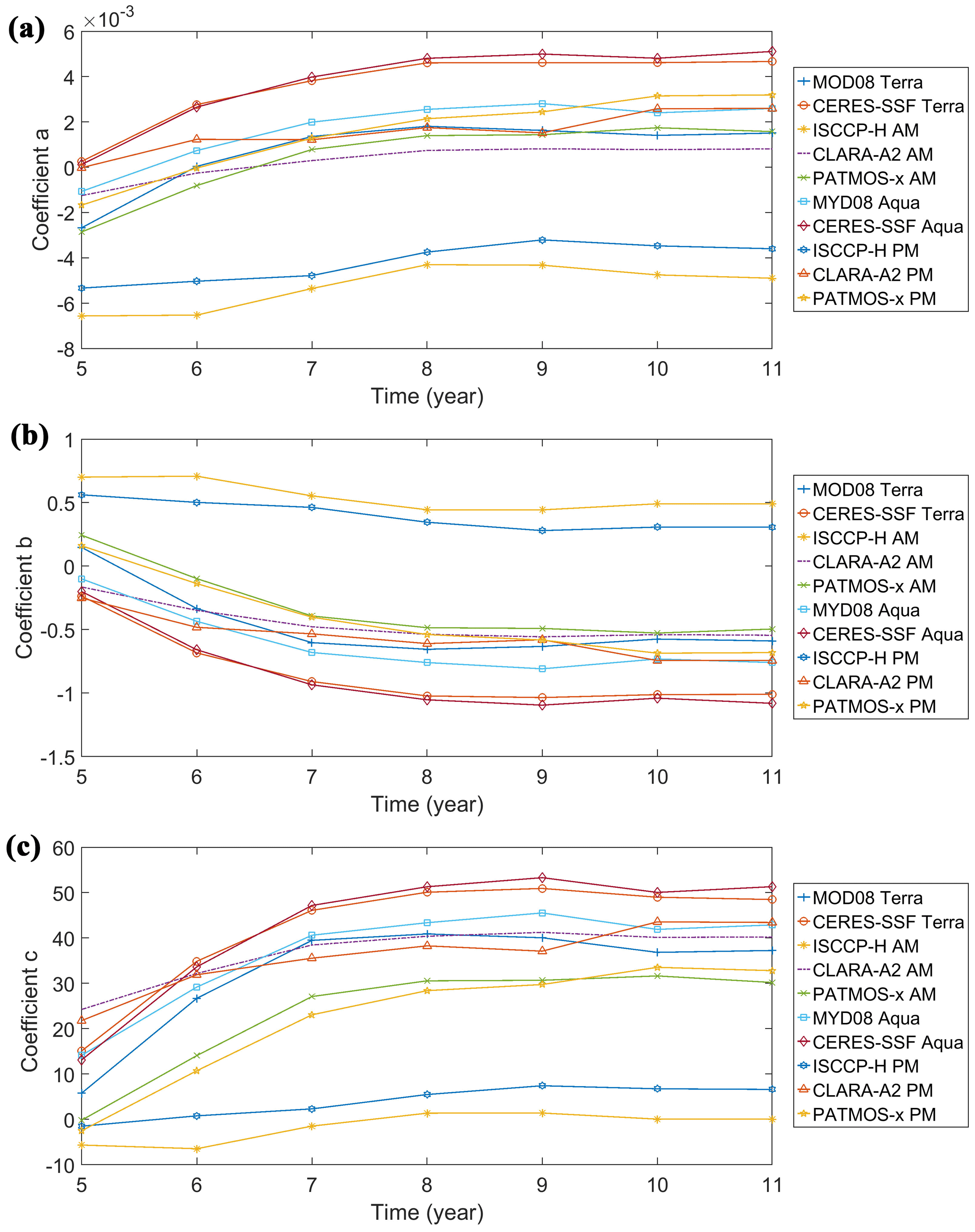
Figure A1 The sensitivity analysis on the CDF matching parameters from the 5th (2011) to the 11th year (2017) of CALIPSO time at 1-year intervals. The coefficients a, b, and c are calculated by the least-square fit method. And the time period only contains sunlit months from April to September.