A long-term 1 km monthly near-surface air temperature dataset over the Tibetan glaciers by fusion of station and satellite observations

Surface air temperature (SAT) is a key indicator of global warming and plays an important role in glacier melting. On the Tibetan Plateau (TP), there exists a large number of glaciers. However, station SAT observations on these glaciers are extremely scarce, and moreover the available ones are characterized by short time series, which substantively hinder our deep understanding of glacier dynamics due to climate changes on the TP. In this study, an ensemble learning model is constructed and trained to estimate glacial SATs with a spatial resolution of 1 km × 1 km from 2002 to 2020 using monthly MODIS land surface temperature products and many auxiliary variables, such as vegetation index, satellite overpass time, and near-surface air pressure. The satellite-estimated glacial SATs are validated against SAT observations at glacier validation stations. Then, long-term (1961–2020) glacial SATs on the TP are reconstructed by temporally extending the satellite SAT estimates through a Bayesian linear regression. The long-term glacial SAT estimates are validated with root mean squared error, mean bias error, and determination coefficient being 1.61 ^∘C, 0.21 ^∘C, and 0.93, respectively. The comparisons are conducted with other satellite SAT estimates and ERA5-Land reanalysis data over the validation glaciers, showing that the accuracy of our satellite glacial SATs and their temporal extensions are both higher. The preliminary analysis illustrates that the glaciers on the TP as a whole have been undergoing fast warming, but the warming exhibits a great spatial heterogeneity. Our dataset can contribute to the monitoring of glaciers' warming, analysis of their evolution, etc. on the TP. The dataset is freely available from the National Tibetan Plateau Data Center at https://doi.org/10.11888/Atmos.tpdc.272550 (Qin, 2022).

1 Introduction

Surface air temperature (SAT) represents the thermal state of the lower atmosphere and serves to regulate the earth surface energy and water budgets and thus impacts the land–atmosphere interaction (Pratap et al., 2019; Huang et al., 2019) and is one of the most important variables in ecology, hydrology, climatology, and environmental sciences (Rasouli et al., 2022; Trebicki, 2020; Box et al., 2019; Huang et al., 2019; Tong et al., 2018). SAT, as a key indicator of global climate change, has been rising rapidly since the industrial revolution, inducing global glacier mass losses (Radić et al., 2014; Hock et al., 2019). The Tibetan Plateau (TP) is the highest plateau in the world, with an average altitude greater than 3500 m and is designated as the roof of the world and the third pole (Yao et al., 2019). At the same time, the TP accommodates the maximum number of glaciers, harboring the largest solid water reserves in the world apart from the polar regions, and is thus named the Asian water tower (Pfeffer et al., 2014; Rounce et al., 2020a; Yao et al., 2012). Similarly, the TP has also been undergoing a warming (Peng et al., 2021) and even exhibits a more intense warming than its surrounding areas (Nie et al., 2021; Lalande et al., 2021; Bhattacharya et al., 2021). This accelerates glacier melt and retreat on the TP (Pratap et al., 2019; Rounce et al., 2020a; Brun et al., 2017; Bhattacharya et al., 2021; Shean et al., 2020; Farinotti et al., 2020), inducing a series of glacial catastrophes, such as glacier lake outburst floods and threatening the neighboring community and infrastructure (Miles et al., 2021; Immerzeel et al., 2020; Kraaijenbrink et al., 2017). So, an extensive monitoring of glacial SATs on the TP is significant for deeply understanding the response of glaciers to climate change and securing the local residents from possible glacial hazards (Guo et al., 2019).

However, knowledge of the spatial patterns of glacial SATs and their changes on the TP has still been full of great uncertainties due to the lack of observations (Rounce et al., 2020b). Almost no station SAT observations were available on the glaciers of the TP in the past, owing to both poor logistics and limited funding (Qin et al., 2009). Many scientists have recently tried to deploy automatic weather stations on the glaciers of the TP to collect meteorological variables including SAT and publicized these field observations (Yang, 2021; Zhang, 2018a, b; Zhao, 2021). On the other hand, it is almost impossible to regularly maintain these instruments due to harsh natural conditions on the glaciers. Thus, the duration of glacial SAT observations is usually relatively short. Moreover, the surface topography of mountain glaciers is often highly uneven, and the weather stations on them are usually set up at their lower parts. Thus, the representativeness of these SAT observations on glaciers is limited, and the thermal status in their other parts is still unclear (Kang et al., 2022; Yang et al., 2014). As to the problem of representativeness, if there are several automatic weather stations in some glacierized basins, the temperature lapse rate (TLR) with respect to increasing elevation is introduced to interpolate station SAT observations to areas on glaciers without stations (Zhang et al., 2021; Rounce et al., 2020a). However, the TLR is unstable and variant in space and time (Li et al., 2013). So, the interpolated SATs via the TLR on the glaciers are full of nontrivial uncertainties (Rounce et al., 2020b). Well known, gridded reanalysis (or simulation) data usually have a long span of time and are thus often taken to address problems of short-term duration (or the nonexistence) of station SAT observations on glaciers (Munoz-Sabater et al., 2021; Harris et al., 2014; Hersbach et al., 2020). However, since the spatial extent of mountain glaciers is normally smaller than that of the grid (about several tens of kilometers), spatial downscaling has to be performed on these gridded data to obtain the distribution of SAT on glaciers, such as through the TLR. In fact, it is reported in many studies that the quality of reanalysis data on the TP is worse, and therefore the reliability of the downscaled SATs based on them is dubious (Li et al., 2013; Wang et al., 2019; You et al., 2010).

Given the strong association between SATs and land surface temperatures (LSTs), attempts have been made to convert satellite LSTs to satellite SATs (Zhang et al., 2016; Shen et al., 2020; Benali et al., 2012; Rao et al., 2019). The methods can generally be divided into four types. The first one is to construct a statistical relationship between SATs and LSTs, as well as other ancillary variables (such as solar zenith angle, elevation, etc.), via a multiple linear regression. This kind of method is simple and can be calibrated with few data. But the relationship between SATs and LSTs is nonlinear, and thus their reliability cannot be guaranteed in some situations. The second kind is called the temperature-vegetation-index method, which is based on the assumption that LST gradually approaches SAT with vegetation coverage increasing. This kind of method is more accurate than the simple linear regression but is susceptible to noise and is inapplicable during the vegetation growing season. The third kind of method constructs a quantitative relationship between SATs and LSTs through a surface energy balance equation, whose advantages are its solid physical basis. However, their accuracy depends strongly on the quality of the inputs, such as soil porosity, which is often difficult to obtain. The fourth one exploits the strong ability of machine learning to capture the nonlinear relationship between SATs and LSTs, as well as other ancillary variables (Xu et al., 2018; Noi et al., 2017; Zeng et al., 2021; Hooker et al., 2018). This kind of method is successfully applied in many regions due to its high accuracy and usability. The machine learning method has also been used to estimate SATs based on satellite LSTs over the TP (Shen et al., 2020; Xu et al., 2018; Zhang et al., 2016). However, the accuracy of these SATs on glaciers is questionable, because the data-driven method needs a huge number of data samples to train them, but the number of station SAT observations on glaciers is rather limited. Furthermore, satellite LSTs of high quality have only been available for the last two decades. Even if the high-quality SATs were estimated on the TP, it would be difficult to use them to analyze climate change on glaciers due to their short-term duration.

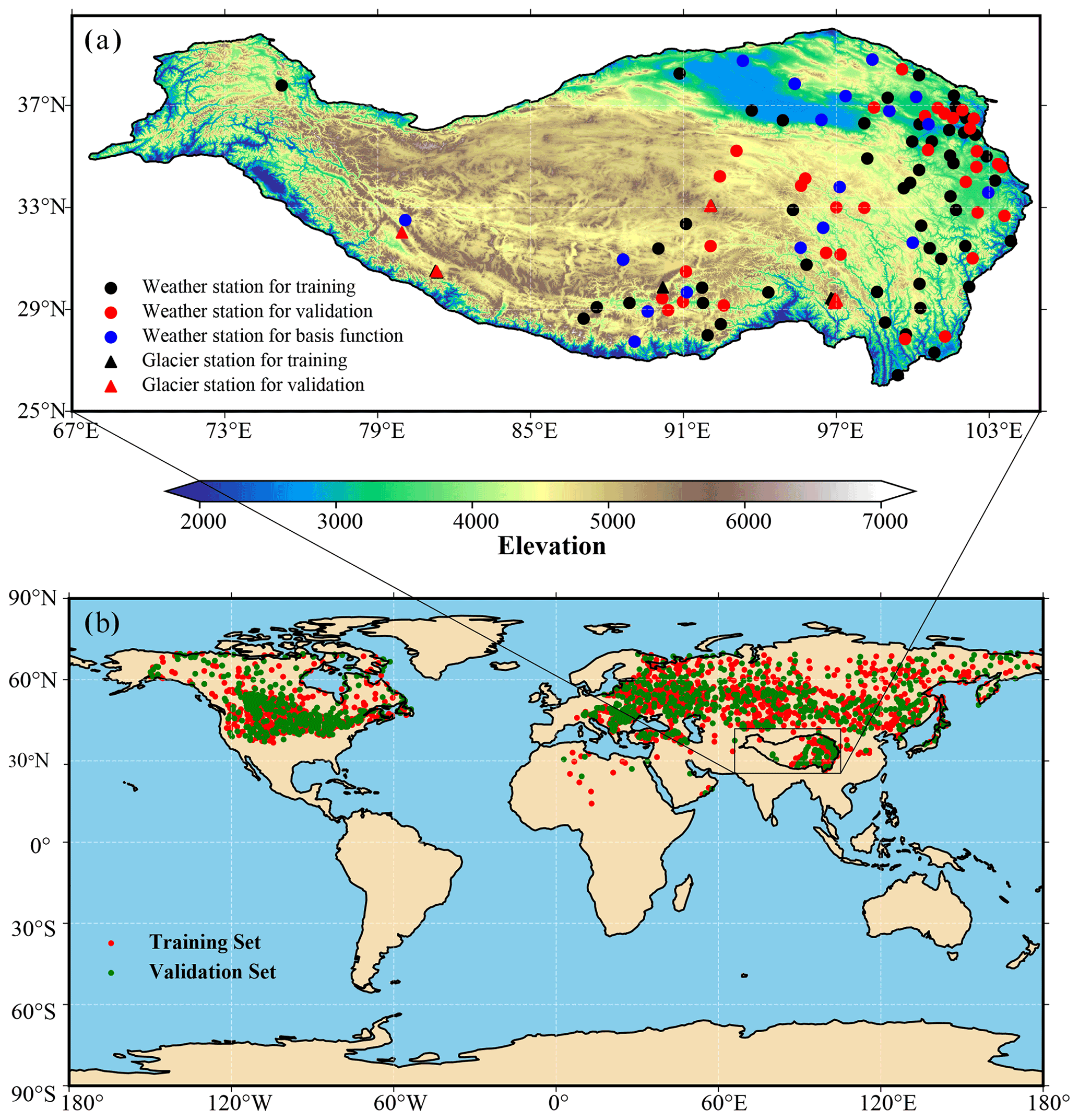
Figure 1 Distribution of used ground observation stations. (a) Meteorological stations from the CMA (black) and stations on glaciers (red) and (b) meteorological stations from the National Centers for Environmental Information of the United States.

In order to address the aforementioned problems, we firstly glean SAT observations from tens of stations on glaciers of the TP, secondly construct a quantitative relationship between station SATs and satellite SATs to obtain short-term glacial SAT estimates through an ensemble learning algorithm, thirdly develop a reconstruction algorithm to temporally extend these satellite SATs to long-term (1961–2020) glacial SATs via a Bayesian linear regression, and finally implement these reconstructed SATs to analyze the glacial warming trends on the TP to illustrate their utility. This article is organized as follows. In Sect. 2, the data sources are shown. Both the method to estimate satellite SATs and the approach to extend them are described in Sect. 3. The results and discussion are given in Sect. 4. Finally, the data availability and the conclusions are presented.

2 Data

2.1 Remote sensing data

A variety of Terra and Aqua MODIS products are used in this study, which are available from the National Aeronautics and Space Administration's (NASA) website (https://earthdata.nasa.gov/, last access: 14 November 2022). The first is the MOD11A1/MYD11A1 product, which provides the daytime and nighttime 1 km LST, satellite overpass time, and quality control indicators for each pixel. Its temporal resolution is 1 d, and the spatial resolution is about 1 km. The second is the enhanced vegetation index (EVI) extracted from the MOD13A3 product. Its temporal and spatial resolutions are 1 month and 1 km, respectively. The third is the shortwave white-sky albedo from the MCD43A3 product, whose temporal and spatial resolutions are 1 d and 500 m, respectively.

2.2 Station products and ancillary data

The station SAT observation datasets used in this study come from three sources. The first one is the 60 years of daily near-surface air temperatures at a total of 145 weather stations on the TP, which are managed by the China Meteorological Administration (CMA), homogenized by Cao et al. (2016), and available from its website (http://data.cma.cn/, last access: 14 November 2022). Their spatial distribution is shown in Fig. 1a (marked by the solid circles). These daily SATs are averaged to obtain monthly ones that match the MODIS monthly LSTs on the time scale. The second one is the glacial SAT observations at 35 automatic weather stations deployed on various glaciers of the TP (marked by the solid triangles in Fig. 1a), including the Naimona'Nyi Glacier in the southwestern part of the TP (Zhang, 2018a), the Kunsha Glacier in the western part of the TP (Zhang, 2018b), the Xiao Dongkemadi Glacier in the central part of the TP (Xu, 2018), and several glaciers in the southeastern part of the TP (Yang, 2021). As aforementioned, a machine learning model is taken to convert LSTs to SATs. Generally, this type of model has a strong capacity. Although approximately a few hundred stations are available over the TP, this number of stations is rather limited in contrast to the vast area of the TP. Thus, the problem of overfitting is likely to occur. In order to mitigate this possible issue, a large number of weather stations in the Northern Hemisphere (outside the TP), which have similar surface conditions to the TP, is selected to enrich the above two data sources. The selection criterion is that the annual mean albedo at these stations is greater than 0.4, because the land on the TP is typically covered by sparse vegetation and ice (snow). The spatial distribution of these selected stations outside the TP is illustrated in Fig. 1b and available from the National Center for Environmental Information of the United States (https://www.ncei.noaa.gov/, last access: 14 November 2022). The most conspicuous feature of the TP is its extremely high elevation. So, the digital elevation model (DEM) data with a spatial resolution of 30 m, which are from the Shuttle Radar Topography Mission (SRTM), are used to reflect this feature. This DEM data can be made available from the United States Geological Survey (USGS) website (https://srtm.csi.cgiar.org/, last access: 14 November 2022). The extent of glaciers on the TP comes from the Randolph Glacier Inventory provided by the National Tibetan Plateau Data Center of China (http://data.tpdc.ac.cn/, last access: 14 November 2022).

3 Methods

3.1 Data preprocessing

Since the purpose of this study is to estimate and reconstruct monthly SATs on glaciers of the TP, both the daily station SAT observations and satellite LSTs are averaged to obtain monthly ones. For weather and glacier stations, all daily SAT observations are simply averaged in 1 calendar month. As to MODIS LST products, the averaging procedure is a little complicated. It is well known that satellite signals are often contaminated by clouds, leading to no LST retrievals or low-quality ones. So, the quality control is conducted on the four daily MODIS LSTs (Terra daytime LST, Terra nighttime LST, Aqua daytime LST, and Aqua nighttime LST) and only the LSTs, whose uncertainties are less than 1 K, are regarded as valid. Then, the averaging procedure is only performed on these LST values for each 1 km pixel on the TP even though only one LST is available in 1 month. Therefore, four monthly MODIS LSTs are calculated. At the same time, the total number of valid daily LSTs in 1 month is used to reflect the cloud information for one pixel and normalized into the range of 0–1. Moreover, four monthly mean satellite overpass times are computed in the same manner and then normalized into the range of 0–1 through being divided by the length of 1 d (24 h). As to MODIS 500 m daily albedos, they are aggregated into a monthly scale by simply averaging, and then they are resampled to a 1 km spatial scale in order to match with the spatial and temporal scales of the other satellite products. For the same reason, the USGS 30 m DEM data are also resampled to a 1 km spatial scale on the TP. As a matter of fact, the DEM data are not used directly but converted into normalized near-surface air pressure belonging to the range of 0–1 as follows:

$$\begin{array}{}\text{(1)}& \mathit{\eta }={\mathrm{10}}^{\left(\frac{-Z}{\mathrm{18}\mathrm{400}}\cdot \frac{\text{LST}}{\mathrm{273}}\right)},\end{array}$$

where η denotes the normalized near-surface air pressure, Z the altitude above sea level (i.e., DEM), and LST the land surface temperature. As pointed out in many studies, both sunrise and sunset times have an impact on the minimum and maximum SATs and their timing. So, these two times are calculated on a daily basis; the monthly averaged ones are simply evaluated in a calendar month and added to the list of input variables for the ensemble learning method.

Figure 2 Procedure to reconstruct 60-year (1961–2020) near-surface air temperature on glaciers.

3.2 Method to convert LSTs to SATs

As aforementioned, a stacking ensemble learning algorithm is constructed to estimate short-term satellite SATs, and then Bayesian linear regression is used to reconstruct long-term glacial SATs. The whole procedure is illustrated in Fig. 2. For estimation, a random forest model, which has been proved effective in many scenarios (Belgiu and Dragut, 2016; Xu et al., 2018), is taken as the base learner and meta learner for ensemble learning. Random forest regression is a supervised machine learning algorithm to merge multiple regression trees to make a more accurate prediction than any individual tree. Its key thought is to perform bootstrap aggregation in both sample and feature dimensions in the learning course. The base learner can be represented as

$$\begin{array}{}\text{(2)}& \text{SAT}=RF\left(\mathit{X}\right),\end{array}$$

where SAT denotes the monthly mean SATs and X the independent variable vector. There are four base learners, corresponding to four MODIS LSTs, and thus there are four input vectors, which can be expressed as follows:

$$\begin{array}{}\text{(3)}& \begin{array}{rl}{X}_{\mathrm{day}}^{\mathrm{terra}}& =\left[{\text{LST}}_{\mathrm{day}}^{\mathrm{terra}},{\mathit{\tau }}_{\mathrm{day}}^{\mathrm{terra}},t_{\mathrm{day}}^{\mathrm{terra}},p_{\mathrm{day}}^{\mathrm{terra}},vi,\mathit{\alpha },t_{\mathrm{sunrise}},t_{\mathrm{sunset}},\cos {\mathit{\theta }}_{\mathrm{sun}}\right],\\ \\ X_{\mathrm{night}}^{\mathrm{terra}}& =\left[{\text{LST}}_{\mathrm{night}}^{\mathrm{terra}},{\mathit{\tau }}_{\mathrm{night}}^{\mathrm{terra}},t_{\mathrm{night}}^{\mathrm{terra}},p_{\mathrm{night}}^{\mathrm{terra}},vi,\mathit{\alpha },t_{\mathrm{sunrise}},t_{\mathrm{sunset}},\cos {\mathit{\theta }}_{\mathrm{sun}}\right],\\ \\ X_{\mathrm{day}}^{\mathrm{aqua}}& =\left[{\text{LST}}_{\mathrm{day}}^{\mathrm{aqua}},{\mathit{\tau }}_{\mathrm{day}}^{\mathrm{aqua}},t_{\mathrm{day}}^{\mathrm{aqua}},p_{\mathrm{day}}^{\mathrm{aqua}},vi,\mathit{\alpha },t_{\mathrm{sunrise}},t_{\mathrm{sunset}},\cos {\mathit{\theta }}_{\mathrm{sun}}\right],\\ \\ X_{\mathrm{night}}^{\mathrm{aqua}}& =\left[{\text{LST}}_{\mathrm{night}}^{\mathrm{aqua}},{\mathit{\tau }}_{\mathrm{night}}^{\mathrm{aqua}},t_{\mathrm{night}}^{\mathrm{aqua}},p_{\mathrm{night}}^{\mathrm{aqua}},vi,\mathit{\alpha },t_{\mathrm{sunrise}},t_{\mathrm{sunset}},\cos {\mathit{\theta }}_{\mathrm{sun}}\right].\end{array}\end{array}$$

Here, the first four terms in the four input vectors (LST, τ, t, and p) denote the MODIS land surface temperature, the clear-sky days, the satellite overpass time, and the air pressure during the daytime and nighttime for the Terra and Aqua satellites, respectively. The other five terms in the vectors (vi, α, t_sunrise, t_sunset, and cos θ_sun) represent the MODIS enhanced vegetation index, the MODIS surface albedo, the sunrise time, the sunset time, and the cosine of sun zenith angle, respectively. Four estimated monthly surface air temperatures ${\mathbf{SAT}}^{\mathrm{est}}={\left[{\text{SAT}}_{\mathrm{day}}^{\mathrm{terra}},{\text{SAT}}_{\mathrm{night}}^{\mathrm{terra}},{\text{SAT}}_{\mathrm{day}}^{\mathrm{aqua}},{\text{SAT}}_{\mathrm{night}}^{\mathrm{aqua}}\right]}^{\mathrm{T}}$ can be procured by plugging the four input vectors ($X_{\mathrm{day}}^{\mathrm{terra}}$, $X_{\mathrm{night}}^{\mathrm{terra}}$, $X_{\mathrm{day}}^{\mathrm{aqua}}$, and $X_{\mathrm{night}}^{\mathrm{aqua}}$) into Eq. (2). The combined surface air temperature SAT^com can be computed through the meta learner as

$$\begin{array}{}\text{(4)}& {\text{SAT}}^{\mathrm{com}}=RF\left({\mathbf{SAT}}^{\mathrm{est}}\right).\end{array}$$

3.3 Temporal reconstruction algorithm

After the satellite SATs have been retrieved by the above ensemble learning algorithm, the temporal extension is performed for each glacial pixel on the TP based on a Bayesian linear regression and can be expressed as

$$\begin{array}{}\text{(5)}& {\text{SAT}}_{\mathrm{h},i}^{\mathrm{ext}}={\mathit{\beta }}_i^{\mathrm{T}}\cdot {\mathbf{SAT}}_h^{\mathrm{obs}},\end{array}$$

where h denotes the time index for the historical period of 1961–2020, ${\text{SAT}}_{\mathrm{h},i}^{\mathrm{ext}}$ the reconstructed historical SATs at pixel i, ${\mathbf{SAT}}_t^{\mathrm{obs}}={\left[\mathrm{1},{\text{SAT}}_{t,\mathrm{1}}^{\mathrm{obs}},{\text{SAT}}_{t,\mathrm{2}}^{\mathrm{obs}},\mathrm{\dots },{\text{SAT}}_{t,N}^{\mathrm{obs}}\right]}^{\mathrm{T}}$ the monthly mean surface air temperature observation at N basis stations, and β_i the vector of extension coefficients. The extension weights are estimated by minimization of the following cost function:

$$\begin{array}{}\text{(6)}& \begin{array}{rl}J& =\sum _{t=\mathrm{1}}^{T_i}\left({\text{SAT}}_{t,i}^{\mathrm{com}}-{\mathit{\beta }}_i^{\mathrm{T}}\cdot {\mathbf{SAT}}_t^{\mathrm{obs}}\right){\mathit{\sigma }}_i^{-\mathrm{2}}\\ & \cdot \left({\text{SAT}}_{t,i}^{\mathrm{com}}-{\mathit{\beta }}_i^{\mathrm{T}}\cdot {\mathbf{SAT}}_t^{\mathrm{obs}}\right)+{\mathit{\lambda }}_i{\mathit{\beta }}_i^{\mathrm{T}}{\mathit{\beta }}_i,\end{array}\end{array}$$

where t denotes the month in the period of 1961–2020, ${\text{SAT}}_{t,i}^{\mathrm{com}}$ the combined SAT for pixel i at time t, σ_i the standard deviation of ${\text{SAT}}_{t,i}^{\mathrm{com}}$, λ_i the regularization parameter to avoid overfitting, and T_i the number of the estimated SATs for pixel i. The specification of σ_i and λ_i has a definitive impact on the estimate of β_i. Here, the variational Bayes method is utilized to optimize the cost function J in order to simultaneously estimate β_i, σ_i, and λ_i (see Qin et al. (2013) for more details).

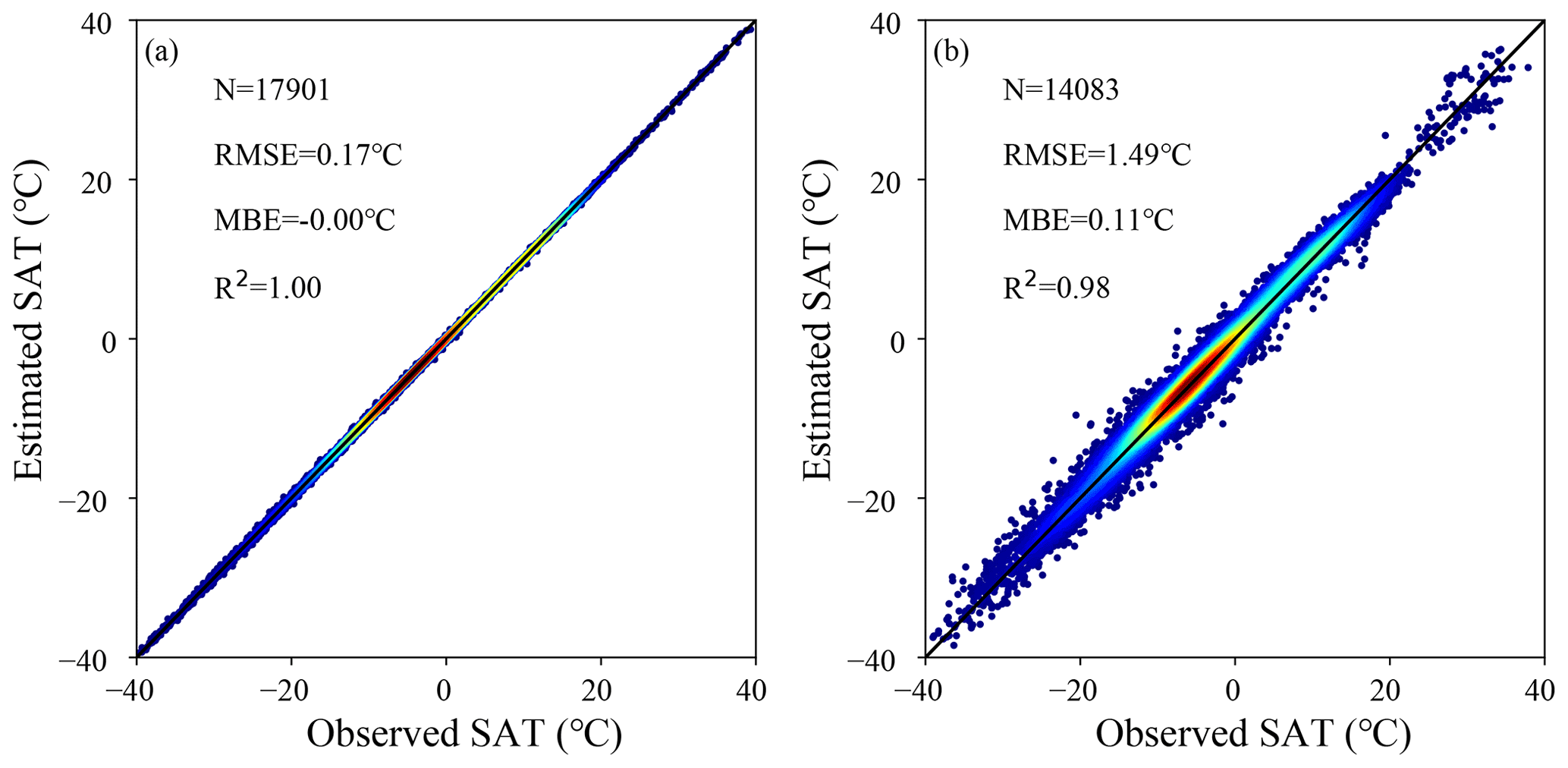
Figure 3 Comparison of observed station SATs with estimated satellite SATs (a) for training and (b) for validation on the whole training and validation datasets.

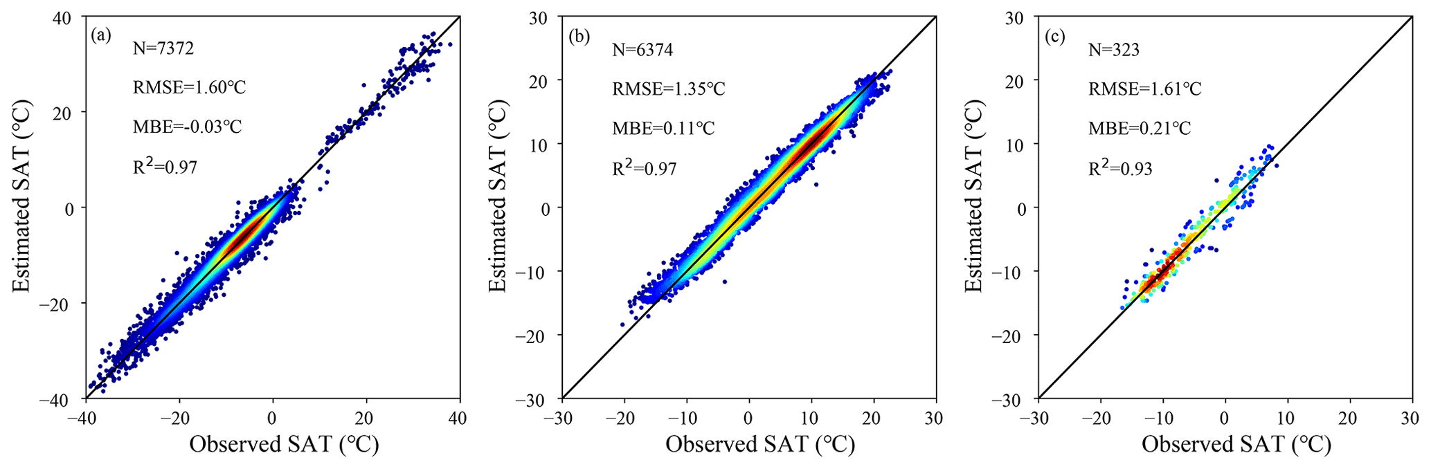
Figure 4 Comparison of observed station SATs with estimated satellite SATs for validation (a) at regular stations in the Northern Hemisphere beyond the Tibetan Plateau, (b) at regular stations on the Tibetan Plateau, and (c) at glacier stations.

3.4 Evaluation indicators

In this study, three error metrics are selected to validate the glacial SAT estimates, which are root mean square error (RMSE), mean bias error (MBE), and determination coefficient (R²). They are expressed as follows:

$$\begin{array}{}\text{(7)}& \begin{array}{l}\text{RMSE}=\sqrt{\frac{\mathrm{1}}{M}\sum _{i=\mathrm{1}}^M{\left(y_i^{\mathrm{est}}-y_i^{\mathrm{obs}}\right)}^{\mathrm{2}}},\\ \text{MBE}=\frac{\mathrm{1}}{M}\sum _{i=\mathrm{1}}^M\left(y_i^{\mathrm{est}}-y_i^{\mathrm{obs}}\right),\\ R^{\mathrm{2}}=\mathrm{1}-\frac{\sum _{i=\mathrm{1}}^M{\left(y_i^{\mathrm{est}}-y_i^{\mathrm{obs}}\right)}^{\mathrm{2}}}{\sum _{i=\mathrm{1}}^M{\left(y_i^{\mathrm{est}}-\stackrel{\mathrm{‾}}{y},\right)}^{\mathrm{2}}}\\ \stackrel{\mathrm{‾}}{y}=\frac{\mathrm{1}}{M}\sum _{i=\mathrm{1}}^M{y}_i^{\mathrm{obs}},\end{array}\end{array}$$

where y^est denotes the estimated SATs (including estimated satellite SATs and reconstructed glacial SATs), $\stackrel{\mathrm{‾}}{y}$ the averaged station SAT observations, and M the number of station observations. When the evaluation is performed according to RMSE, MBE, and R², it often happens that RMSE, MBE, and R² exhibit inconsistencies. For example, the RMSE of one dataset is larger than the RMSE of the other dataset, but R² is also larger than R² of the other dataset. Here, a comprehensive error metric (DISO) is introduced to handle this and can be formulated as (Zhou et al., 2021)

$$\begin{array}{}\text{(8)}& \text{DISO}=\sqrt{{\left(R-\mathrm{1}\right)}^{\mathrm{2}}+{\left(\text{RMSE}/\stackrel{\mathrm{‾}}{y}\right)}^{\mathrm{2}}+{\left(\text{RMSE}/\stackrel{\mathrm{‾}}{y}\right)}^{\mathrm{2}}}.\end{array}$$

Overall, the smaller DISO is, the better estimates are.

Figure 5 Comparison between station SAT observations and satellite SAT estimates over glaciers for (a) our products and (b) Xu's products (Xu et al., 2018). There is a total of 182 sample points, since the overlay period of these two datasets is from 2002 to 2015.

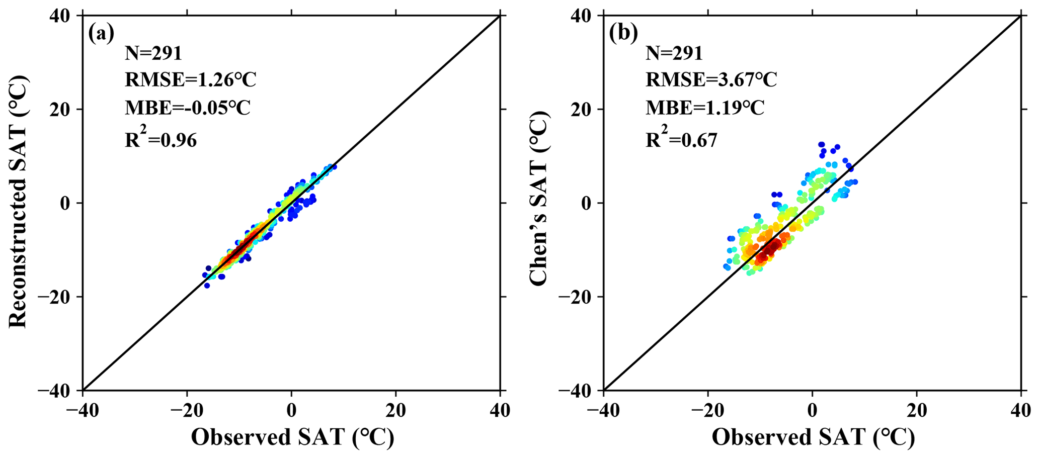
Figure 6 Comparison between station SAT observations and satellite SAT estimates over glaciers for (a) our products and (b) Chen's products (Chen et al., 2021). There is a total of 291 sample points, since the overlay period of these two datasets is from 2002 to 2019.

4 Results and discussion

4.1 Evaluation of satellite SATs

Figure 3a shows the overall training results for the presented ensemble learning algorithm. There is a total of 17 901 samples from July 2002 to December 2020 in the training dataset (in synchronization with the time span of MODIS). As can be seen, the training accuracy can attain an extremely high level with RMSE, MBE, and R² being equal to 0.17 ^∘C, 0.00 ^∘C, and 1.00 ^∘C, respectively. This indicates the strong capability of the ensemble leaning algorithm to capture the variation in the samples. As a matter of fact, more attention should be paid to the validation results. Figure 3b shows the overall validation results with RMSE, MBE, and R² being equal to 1.47 ^∘C, 0.11 ^∘C, and 0.98 ^∘C, respectively. Although the overall validation accuracy is inferior to the overall training accuracy, the validation results are fairly favorable. Moreover, the validation results are illustrated in three groups of stations in Fig. 4. As shown in Fig. 4a, the validation results at global regular stations outside the TP are similar to the overall validation results with RMSE, MBE, and R² being equal to 1.60 ^∘C, −0.03 ^∘C, and 0.97 ^∘C, respectively. For regular stations in the TP, RMSE, MBE, and R² are equal to 1.35 ^∘C, 0.11 ^∘C, and 0.97 ^∘C, respectively. For only glaciers, the validation results are slightly worse than those at regular stations, with RMSE, MBE, and R² being equal to 1.61 ^∘C, 0.21 ^∘C, and 0.93 ^∘C, respectively. The total number of glacier stations for validation is 18, and the validation results for each station are listed in Table 1. It can be seen that most of the glacier stations were set up in 2018, and their observation periods lasted less than 2 years. Moreover, the number of high-quality monthly SAT observations is rather limited, and only one observation sample is available at two stations (SETP12 and SETP13; see Table 1) due to harsh natural conditions. Only SETP1 has a long observation period lasting for approximately 15 years.

Table 1 Validation results for each glacier station on the TP.

To further examine the reliability of the satellite SAT estimates on glaciers, comparisons with three other SAT datasets are performed. Two of them are the satellite SAT datasets based on MODIS LST products compared with machine learning methods (Xu et al., 2018; Chen et al., 2021), which cover the periods of 2001–2015 and 2001–2019, respectively, with a spatial resolution of 1 km × 1 km. As can be seen in Fig. 5, Xu's SAT product has a RMSE, MBE, and R² of 3.11 ^∘C, 0.84 ^∘C, and 0.81 ^∘C, respectively, over the glaciers. However, three error metrics for our glacial satellite SAT product are equal to 1.34 ^∘C, −0.13 ^∘C, and 0.96 ^∘C, obviously being superior to those of Xu's SAT products. As for Chen's product, the error metrics are 3.67 ^∘C, 1.19 ^∘C, and 0.67 ^∘C, respectively, being inferior to ours as indicated in Fig. 6.

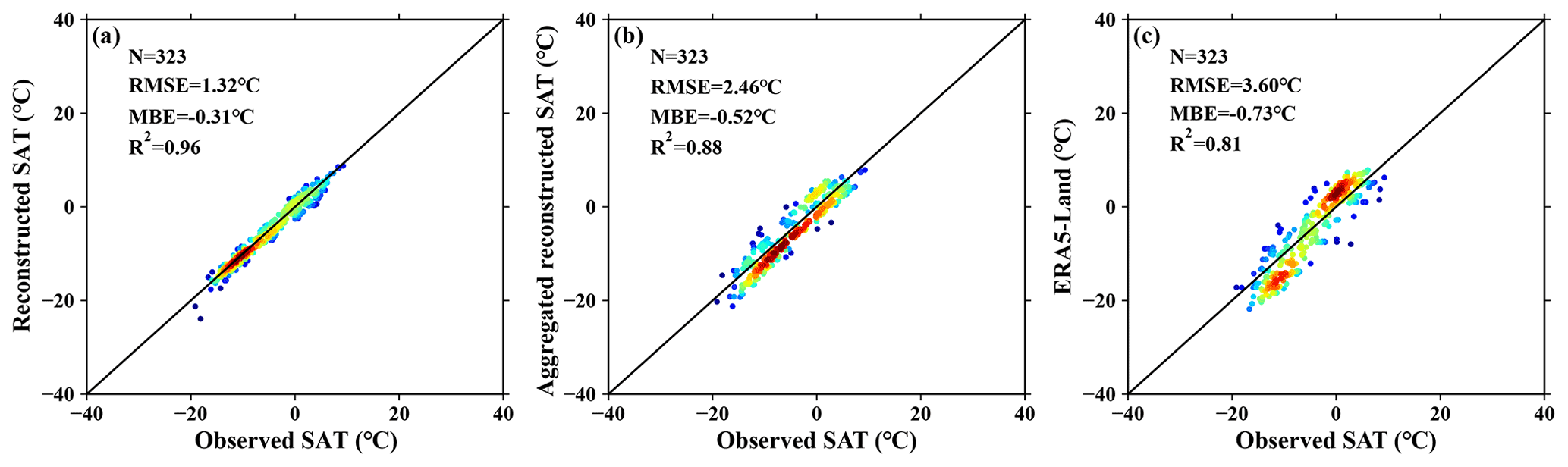
Figure 7 Comparison between station SAT observations and satellite SAT estimates over glaciers for (a) our SAT products at a spatial resolution of 1 km × 1 km, (b) our products aggregated to a resolution of ERA5-Land at 0.1^∘, and (c) ERA5-Land SATs. There is a total of 323 sample points, since the overlay period of these two datasets is from 2002 to 2020.

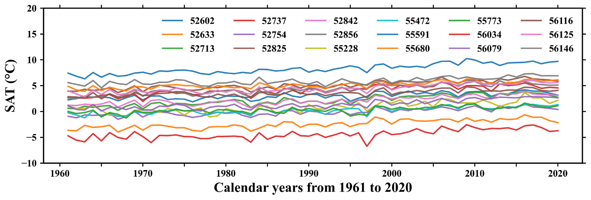
Figure 8 Surface air temperature time series from 1961 to 2020 at 18 stations selected as basis functions for reconstruction.

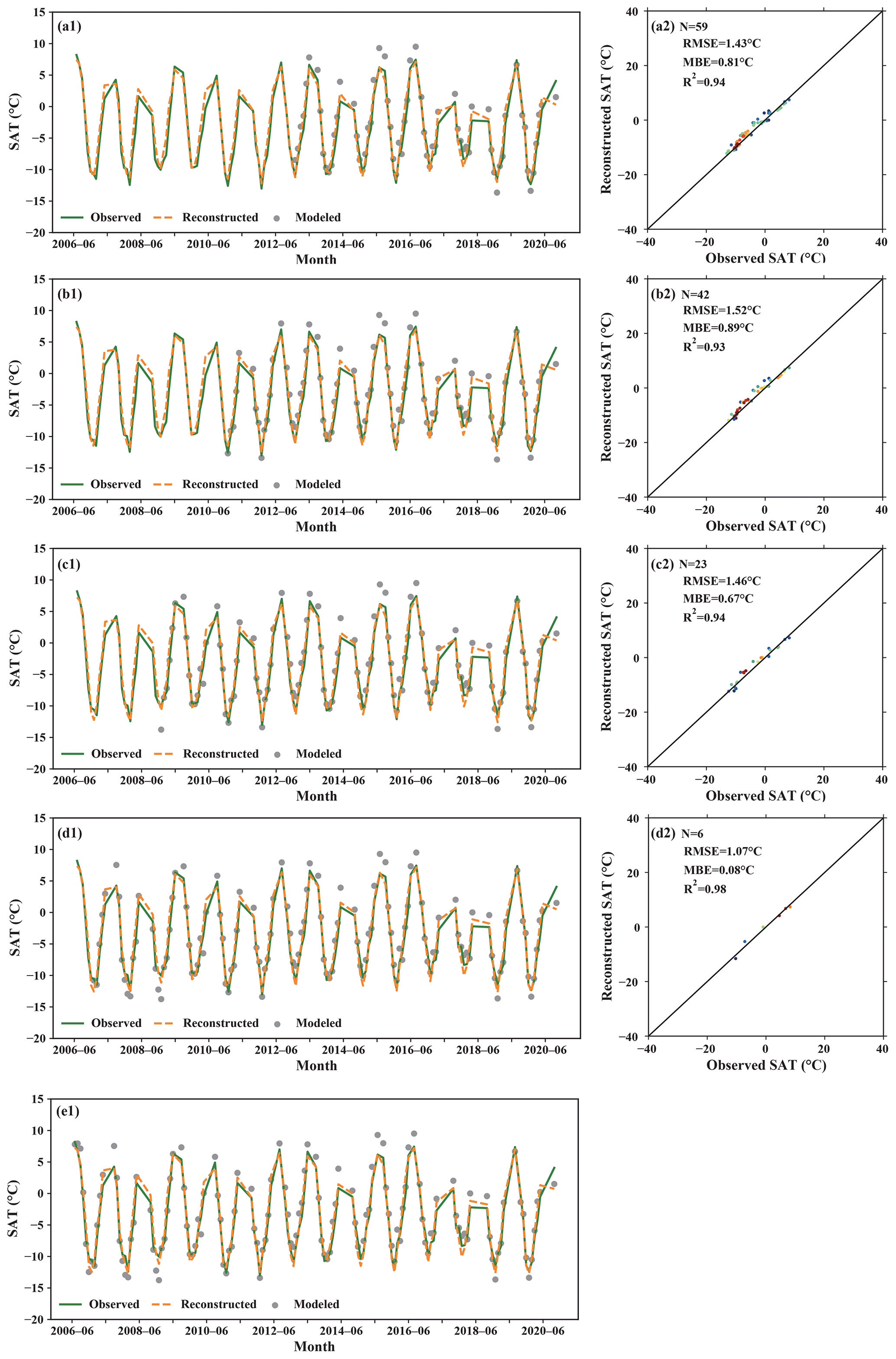
Figure 9 Validation of reconstructed SATs at glacier station SETP1 in five ideal experiments with various specified periods in which satellite SAT estimates are available. (a) For the periods of 2013 to 2020, (b) 2011 to 2020, (c) 2009 to 2020, (d) 2007 to 2020, and (e) 2005 to 2020.

The other comparison is the ERA5-Land reanalysis dataset. It has a spatial resolution of 0.1^∘ and a time span from 1951 to the present. As can be seen in Fig. 7a and c, the performance of our SAT products significantly surpasses the one of ERA5-Land, since RMSE, MBE, and R² deteriorate from 1.32 ^∘C, −0.31 ^∘C, 0.96 to 3.60 ^∘C, −0.71 ^∘C, and 0.81 ^∘C. At the same time, the satellite SAT estimates at a 1 km × 1 km resolution are aggregated to the ones at a 0.1^∘ resolution and then compared with the corresponding ERA5-Land products in order to investigate whether or not the inferiority of ERA5-Land SATs over the glaciers is caused by the difference in the spatial scale. It is illustrated in Fig. 7b that the aggregated SATs are also superior to the ERA5-Land ones over the glaciers with RMSE, MBE, and R² equal to 2.46 ^∘C, −0.52 ^∘C, and 0.88 ^∘C. This proves the advantage of the presented satellite SAT retrieval algorithm itself after adding the samples over glaciers into the estimation model.

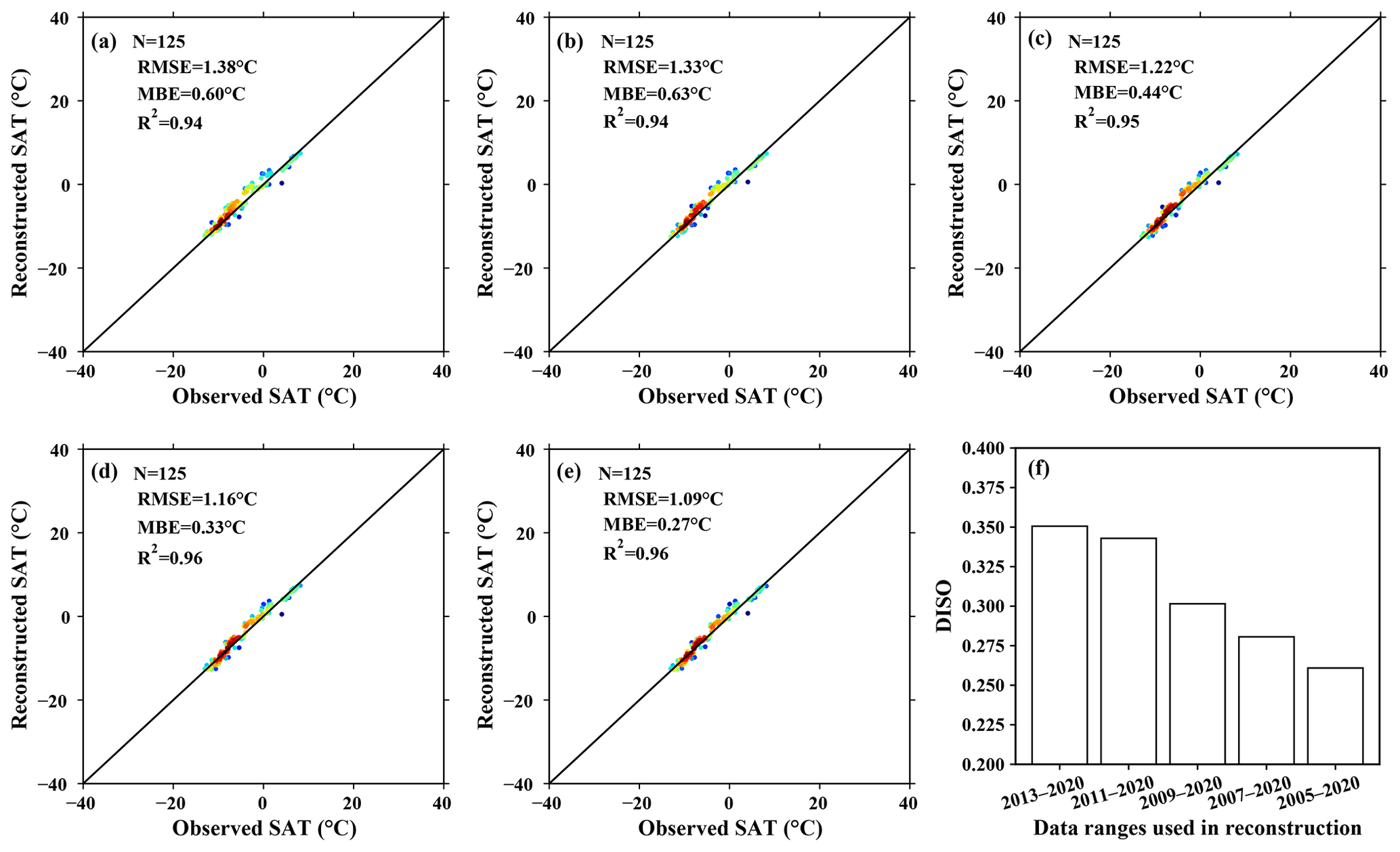
Figure 10 Comparison between observed SATs and reconstructed SATs in the period of 2006 to 2020 at glacier station SETP1 in five ideal experiments with various specified periods in which satellite SAT estimates are available. (a) For the periods of 2013 to 2020, (b) 2011 to 2020, (c) 2009 to 2020, (d) 2007 to 2020, and (e) 2005 to 2020 and (f) for the error metric DISO in the five experiments.

Figure 11 Warming trends over glaciers of the Tibetan Plateau from 1961–2020. (a) Annual anomalies of surface air temperatures over all glaciers and (b) spatial pattern of glacial warming trends.

4.2 Evaluation of reconstructed glacial SATs

The primary goal of this study is to reconstruct long-term glacial SATs to deepen our understanding of the glacial warming status on the TP. As mentioned in Sect. 3.3, long-term continuous SAT observations at some stations need to be selected as basis functions. In principle, the more the number of basis functions, the better the reconstructed results. In fact, the number of such basis functions is scant, because harsh natural conditions often cause failure of measuring instruments and thus observations are missed. So, a total of 18 regular weather stations, at which there are no missing observations in 1961–2020, are selected out of 145 stations as basis functions (Fig. 8). It is notable that the temporal extension is performed on a monthly basis, and the annually averaged values are just presented for illustration. As can be seen, the spatial variabilities of these basis functions are rather striking (Fig. 1), but the temporal variabilities show similarities to some degree. For example, the SAT differences between stations 52 062 and 56 034 can attain more than 12.0 ^∘C due to their distinct elevations and long distance. Before the reconstruction is performed for every glacier pixel, five ideal experiments are conducted at the pixel, where the glacier station SETP1 is located, in order to substantiate the efficacy of the reconstruction algorithm. The procedure for each experiment consists of three steps. Firstly, the observation period (2006–2020) is partitioned into two parts. Secondly, the glacial satellite SAT estimates in the later part are used to evaluate the extension coefficients β in Eq. (5). Thirdly, the glacial station SAT observations in the earlier part are used to validate the reconstructed SATs. The difference among these five experiments lies in the various years to separate the observation period. The separation years are 2013, 2011, 2009, 2007, and 2005. As can be seen in Fig. 9a1, b1, c1, c1, and e1, the number of satellite SAT estimates, which is used to compute the extension coefficients, increases with the separation year moving forward, and accordingly the number of station SAT observations declines. At the same time, the validation accuracy (RMSE, MBE, and R²) gradually improves in the first four experiments as shown in Fig. 9a2, b2, c2, and d2. It is notable that no validation is performed for the fifth experiment, since the separation year of 2005 means that all satellite SAT estimates in the observation period are used in evaluating the extension coefficients.

As a matter of fact, in the five ideal experiments, the temporal extension process can produce not only the reconstructed SATs in the time period in which no satellite SAT estimates exist but also the ones in the period when satellite SATs are available. These reconstructed SATs in the latter period can be regarded as being smoothed. Figure 10a–e illustrates the comparison between all reconstructed SATs and observed SATs for the five ideal experiments. As shown in Fig. 10f, the comprehensive error metric (DISO) becomes better with the number of satellite SAT estimates rising. The ideal experiments are performed only at one glacier station with a long-term series of observations, and such experiments cannot be done at other glacier stations due to the lack of SAT observations. However, these ideal experiments demonstrate that the presented reconstruction algorithm can restore the historical SATs on glaciers with high accuracy.

4.3 Glacial warming pattern

Both annual means and anomalies of reconstructed SATs at each glaciated pixel are calculated for the period of 1961 to 2020. Then, the anomalies are averaged over all glaciated pixels to obtain the holistic warming trend of the glaciated area on the TP. As can be seen in Fig. 11a, the glaciated areas on the TP have undergone rapid warming in the past 60 years with a warming rate of 0.024 ^∘C yr⁻¹ at the 95 % confidence level. It is also found that the coldest and warmest SATs occur in 1967 and 2016 with averaged values of −11.20 ^∘C and −9.33 ^∘C, respectively. In order to obtain a complete understanding of the warming pattern in space, the warming trends for each glaciated pixel are illustrated in Fig. 11b. Except for a few glaciers in the southeast, the warming happens over almost all glaciers on the TP but at the same time exhibits a spatial heterogeneity, being more pronounced in the north. The maximum warming rate reaches 0.07^∘C yr⁻¹, appearing over the glaciers in the central Karakorum Mountains located in the northwestern part of the TP. The cooling occurs over the glaciers of the western Himalayas in the southwest of the TP and the glaciers of the Nyainqentanglha Mountains in the south of the TP, but the cooling trends are not significant.

5 Data availability

The 60-year (1961–2020) glacial near-surface air temperature dataset on the Tibetan Plateau is freely available from the National Tibetan Plateau Data Center at https://doi.org/10.11888/Atmos.tpdc.272550 (Qin, 2022). The dataset provides monthly estimates of near-surface air temperature within 67.67–104.67^∘ E and 26.01–40.00^∘ N at a spatial resolution of 1 km in units of ^∘C. All files are stored in GeoTIFF format with a datum of WGS84. Each file is named “yyyymm.tif”, where “yyyy” and “mm” denote year and month, respectively. For example, the file “196101.tif” stores the glacial monthly near-surface air temperature on the Tibetan Plateau in January 1961.

6 Summary

The shortage of long-term glacial SATs with high spatial resolution has seriously hindered a deep understanding of the glacial warming status on the TP. On the basis of MODIS LST products and station SAT observations, we develop an ensemble learning algorithm with a random forest being the base learner to convert MODIS LSTs to SATs over the glaciers of the TP from 2002 to 2020. The glacial satellite SAT estimates are validated against glacial station SAT observations with RMSE, MBE, and R² equal to 1.61 ^∘C, 0.21 ^∘C, and 0.93 ^∘C, respectively. At the same time, a series of experiments are conducted to corroborate the effectiveness of the temporal extension algorithm. Afterwards, long-term SATs between 1961 and 2020 are reconstructed for all the glacier pixels over the TP. Based on the reconstructed SATs, the warming trend from 1961 to 2020 over all the glaciers of the TP is equal to 0.024 ^∘C yr⁻¹ in the past 60 years. The spatial warming pattern indicates that most of the glaciers are undergoing a warming process with a maximum warming rate of 0.07 ^∘C yr⁻¹, and only a few glaciers in the southeastern part of the TP exhibit an insignificant cooling trend. Overall, this study alleviates the problem of being short of long-term SAT data over the glaciers of the TP. The reconstructed SAT dataset can strongly underpin climate change and modeling research on glaciers of the TP. In the future, we intend to enhance the temporal resolution of the glacial SAT dataset to a daily scale and implement the spatial extension outside of the TP to other ice-covered areas in the world, such as the North and South poles.