the Creative Commons Attribution 4.0 License.
the Creative Commons Attribution 4.0 License.
 | 18 Jan 2023
AI4Boundaries: an open AI-ready dataset to map field boundaries with Sentinel-2 and aerial photography
Raphaël d'Andrimont
Martin Claverie
Pieter Kempeneers
Davide Muraro
Momchil Yordanov
Devis Peressutti
Matej Batič
François Waldner
Field boundaries are at the core of many agricultural applications and are a key enabler for the operational monitoring of agricultural production to support food security. Recent scientific progress in deep learning methods has highlighted the capacity to extract field boundaries from satellite and aerial images with a clear improvement from object-based image analysis (e.g. multiresolution segmentation) or conventional filters (e.g. Sobel filters). However, these methods need labels to be trained on. So far, no standard data set exists to easily and robustly benchmark models and progress the state of the art. The absence of such benchmark data further impedes proper comparison against existing methods. Besides, there is no consensus on which evaluation metrics should be reported (both at the pixel and field levels). As a result, it is currently impossible to compare and benchmark new and existing methods. To fill these gaps, we introduce AI4Boundaries, a data set of images and labels readily usable to train and compare models on field boundary detection. AI4Boundaries includes two specific data sets: (i) a 10 m Sentinel-2 monthly composites for large-scale analyses in retrospect and (ii) a 1 m orthophoto data set for regional-scale analyses, such as the automatic extraction of Geospatial Aid Application (GSAA). All labels have been sourced from GSAA data that have been made openly available (Austria, Catalonia, France, Luxembourg, the Netherlands, Slovenia, and Sweden) for 2019, representing 14.8 M parcels covering 376 K km2. Data were selected following a stratified random sampling drawn based on two landscape fragmentation metrics, the perimeter/area ratio and the area covered by parcels, thus considering the diversity of the agricultural landscapes. The resulting “AI4Boundaries” dataset consists of 7831 samples of 256 by 256 pixels for the 10 m Sentinel-2 dataset and of 512 by 512 pixels for the 1 m aerial orthophoto. Both datasets are provided with the corresponding vector ground-truth parcel delineation (2.5 M parcels covering 47 105 km2), and with a raster version already pre-processed and ready to use. Besides providing this open dataset to foster computer vision developments of parcel delineation methods, we discuss the perspectives and limitations of the dataset for various types of applications in the agriculture domain and consider possible further improvements. The data are available on the JRC Open Data Catalogue: http://data.europa.eu/89h/0e79ce5d-e4c8-4721-8773-59a4acf2c9c9 (European Commission, Joint Research Centre, 2022).
- Article
(12465 KB) - Full-text XML
- BibTeX
- EndNote


Field boundaries are at the core of many agricultural applications such as mapping crop types and yield estimation. With the development of digital farming platforms, extracting and updating field boundaries automatically has gained much traction to facilitate customer onboarding. Different spatial and temporal data coverage could be needed according to the desired application.
There are three broad methods to map field boundaries: deep learning, object-based image segmentation, and conventional (edge-detection) filters (Waldner and Diakogiannis, 2020). Deep learning methods can extract field boundaries from satellite/aerial images better than object-based image analysis (e.g. multiresolution segmentation) or conventional filters (Sobel filters) because they can learn to emphasise relevant image edges while suppressing others. For instance, Waldner and Diakogiannis (2020) and Waldner et al. (2021) have shown that convolutional neural networks can learn complex hierarchical contextual features from the image to accurately detect field boundaries and discard irrelevant boundaries, thereby outperforming conventional edge filters. More recently, a similar approach has been used to unlock large-scale crop field delineation in smallholder farming systems with transfer learning and weak supervision (Wang et al., 2022). Deep learning methods need labels for training and evaluation. No benchmark data set exists to easily do so. The absence of such benchmark data impedes proper comparison with existing methods. Besides, there is no consensus on which evaluation metrics should be reported (both at the pixel and field levels). As a result, it is currently challenging to benchmark new and existing methods.
Deep learning parcel delineation based on the land parcel identification system has been evaluated in several countries such as France (Aung et al., 2020), Netherlands (Masoud et al., 2019), and Spain (Garcia-Pedrero et al., 2019). However, as there is no European harmonised land parcel identification system, there is no dataset to properly benchmark methods over a variety of landscapes and latitudes.
The Geospatial Aid Application (GSAA) refers to the annual crop declarations made by European farmers for Common Agricultural Policy (CAP) area-aid support measures. The electronic GSAA records include a spatial delineation of the parcels. A GSAA element is always a polygon of an agricultural parcel with one crop (or a single crop group with the same payment eligibility). The GSAA is operated at the region or country level in the European Union's (EU) 28 Member States (MS), resulting in about 65 different designs and implementation schemes over the EU. Since these infrastructures are set up in each region, data are not interoperable at the moment, and the legends are not semantically harmonised. Furthermore, most GSAA data are not publicly available, although several countries are increasingly opening the data for public use. In this study, seven regions with publicly available GSAA are selected, representing a contrasting gradient across the European Union (i.e. agricultural system depends on physical and human geography resulting in contrasted landscapes). More detailed information about the GSAA is provided in the Sect. 2.3.
Creating reference AI data sets in remote sensing has been shown to accelerate method development and to help push the boundary of the state of the art. For instance, data sets such as BigEarthNet (Sumbul et al., 2019) and EuroSAT (Helber et al., 2019) have been used for generic land cover. For agriculture, most of the previously published datasets over Europe are focusing on France (BreizhCrop and PASTIS; Rußwurm et al., 2019; Tarasiou et al., 2021) or France and Catalonia (Sen4AgriNet; Sykas et al., 2022). In addition to the fact that no harmonised dataset is currently available for multiple European countries, no dataset combining remote sensing and very high-resolution aerial imagery has yet to be published.
To fill these gaps, we release two AI-ready data sets (pairs of images and labels) for field boundary detection to facilitate model development and comparison, as follows:
-
A multi-date dataset based on Sentinel-2 monthly composites for large-scale analyses in retrospect.
-
A single-date dataset based on orthophoto for regional-scale analyses such as the automation of GSAA.
All labels are sourced from public parcel data (GSAA) that have been made openly available.
2.1 Sampling
The rationale behind this study is to propose ready-to-use data set of Earth observation data with corresponding parcel boundaries. Public parcel data are first obtained over several countries/regions (i.e. Austria, Catalonia, France, Luxembourg, Netherlands, Slovenia, and Sweden) for the year 2019. After drawing a grid of cells of 4 by 4 km in the ETRS89-extended LAEA Europe projection (EPSG:3035), a stratified random sampling is drawn based on the following two variables:
-
the average parcel perimeter/area ratio (PAR) computed for each cell is then distributed over 5 percentile bins,
-
the coverage percentage of parcels within the cell distributed in 10 classes.
We designed a random stratified sampling method to extract the image chips from various landscapes. First, the 4×4 km grid was overlaid over each country/region where parcel data are available. In each grid cell, the field fraction (in percent) and the perimeter/area ratio were computed as shown for France in Fig. 1. These indicators jointly describe the prevalence of agriculture (i.e. land proportion covered by agriculture) and the landscape fragmentation (i.e. perimeter area ratio) of each grid cell. Fifty strata were defined by discretising the field fraction in 10 classes (from 0 % to 100 % by step of 10 %) and the perimeter area ratio in 5 classes defined by its 20th percentile in order to obtain a representative sampling. The goal was to sample 85 000 sampling units representing an already important dataset to train deep learning models. To this aim, 170 sampling were selected per stratum (Fig. 2). In those strata where the number of samples is larger than the number of available grid cells, the sampling units in excess were evenly distributed to the other strata. Within each stratum, grid cells were selected so as to maximise the balance between source regions.
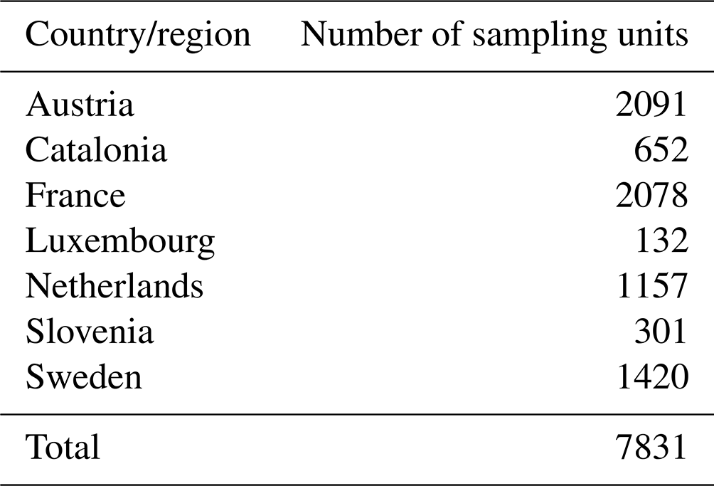
The resulting sampling results in 7831 samples distributed as described in Table 1 and in Fig. 3.
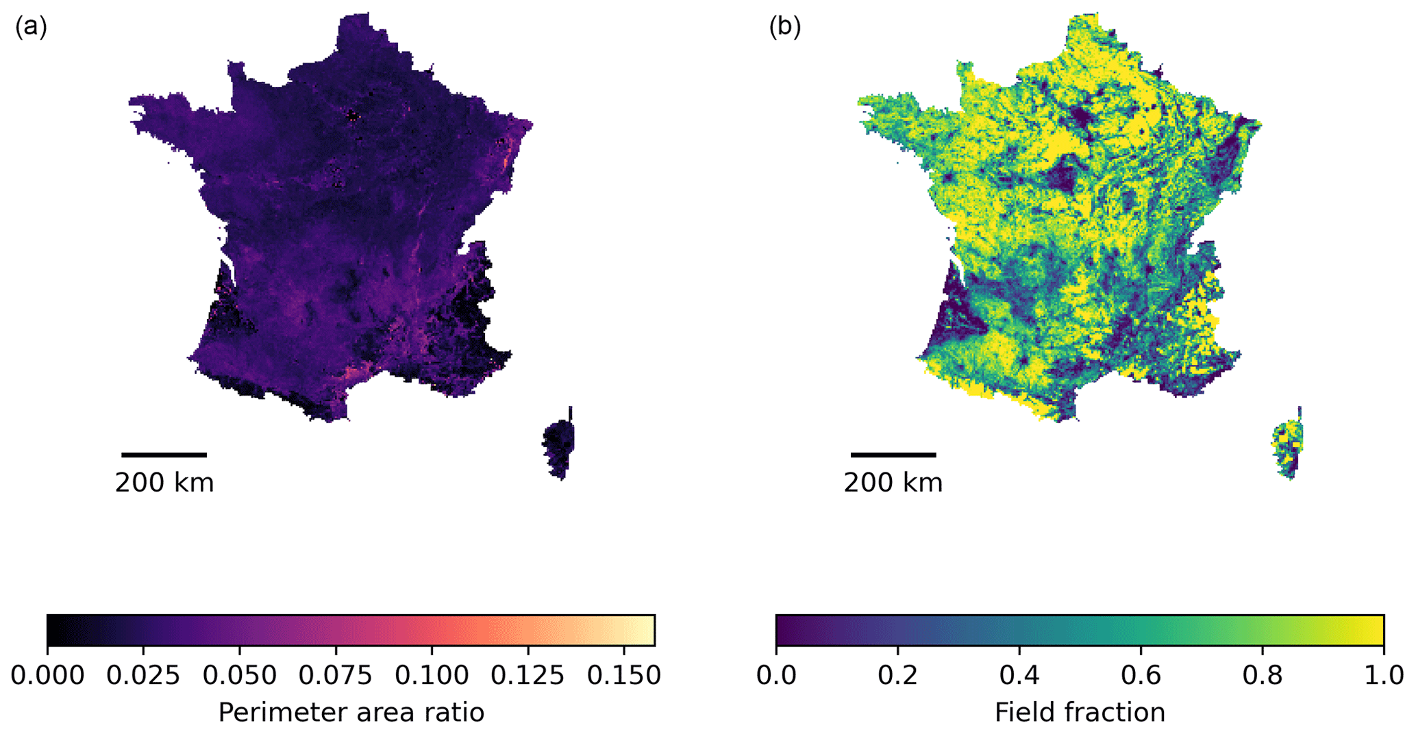
Figure 1The stratification of the sampling is done based on perimeter area ratio (a) and proportion of parcels (b) in 4 km × 4 km grid cells. Example across France.
Table 1Distribution of the final stratified sampling for each region.
The samples are mainly distributed from North to South (Fig. 3).
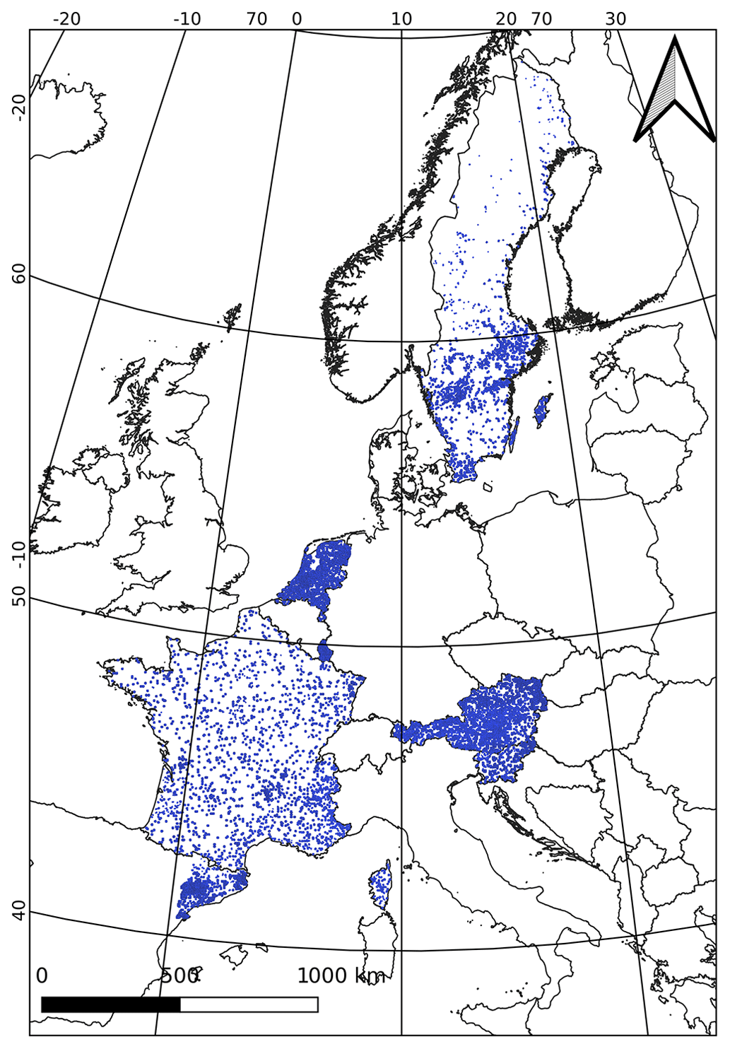
Figure 3Spatial distribution of sampling units among the seven regions.
2.2 Earth observation (EO) data
Image chips of a fixed pixel size are required to feed deep learning models. EO data were extracted for the two specific datasets, as shown in Fig. 4:
-
Sentinel-2 monthly composites (March to August 2019), 256 by 256 pixels,
-
Orthophoto single-temporal imagery resampled at 1 m resolution, 512 by 512 pixels.
The difference in pixel extent (256 vs. 512) of the two datasets is linked to the spatial resolution of Sentinel-2 (10 m) and orthophoto (1 m), respectively, corresponding thus to 2560 m by 2560 m and 512 m by 512 m. The extent of the orthophoto extracted has to be extended from 256 to 512 to provide sufficient context.
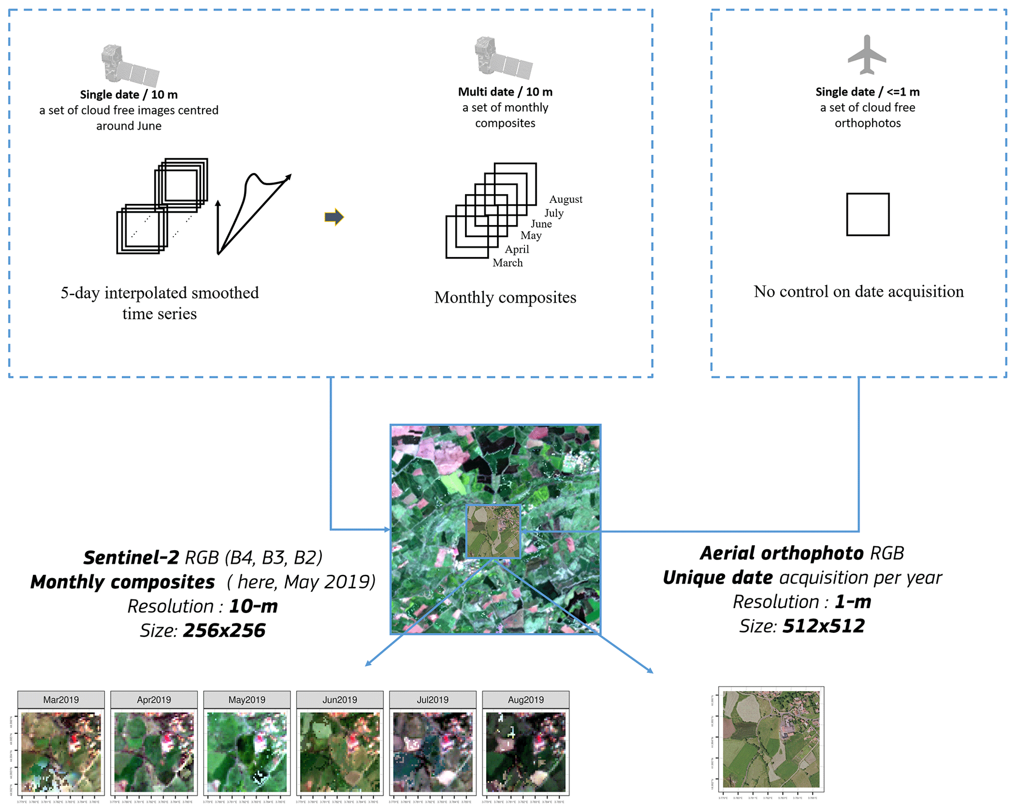
Figure 4Earth observation generation overview. Sentinel-2 time series' are interpolated and smoothed to generate 10 m monthly composites cropped on 256 by 256 pixels. Aerial orthophotos are resampled at 1 m and cropped on 512 by 512 pixels in the center of the 4 km sampled cell. The Sentinel-2 time series cropped to the orthophoto extent is shown in detail in Fig. A2.
2.2.1 Sentinel-2
This section describes how the monthly cloud-free Sentinel-2 surface reflectance composites for March to August 2019 (thus 6 months of four bands: R, G, B, NIR) were produced. Figure 5 provides an example of the dataset.
The Sentinel-2 level-2A surface reflectance (SR) were derived from the Sentinel-2 level-1C top of atmosphere (TOA) reflectance data processed using the Sen2Cor processor (Main-Knorn et al., 2017) from the ESA SNAP toolbox (European Space Agency, 2023). The four spectral bands that are available at a spatial resolution of 10 m were selected (B2, B3, B4, and B8). The Scene Classification Layer (SCL) obtained from Sen2Cor was added as an extra band. Sentinel-2 processing was performed on the BDAP (Soille et al., 2018) using the open-source pyjeo (Kempeneers et al., 2019) Python package.
Data cubes, consisting of merging all 2019 acquisitions for all 4×4 km2 chips, were created. The data cubes were extended with the acquisitions of the preceding (December 2018) and successive (January 2020) months. The extra observations served to mitigate the boundary effects at the beginning and end of the time series while applying temporal operations. These months were removed after the filter was applied.
Only pixels identified as dark (SCL = 2), vegetated (SCL = 4), not-vegetated (SCL = 5), water (SCL = 6), and unclassified (SCL = 7) were considered as “clear”. In addition, outliers were detected using the Hampel identifier (Hampel, 1974), based on the pixel values in the red (B4) and near-infrared (B8) bands. The SCL was resampled to 10 m based on the nearest neighbour to obtain a regular gridded data cube. The Hampel filter calculates the median and the standard deviation in a moving window, expressed as the median absolute deviation (MAD). For the moving window, a width of 40 d was considered. Pixels below 2 and above 3 standard deviations from the median were identified as outliers for the NIR and the red bands, respectively. The respective values of 2 and 3 standard deviations for the lower and upper bounds were selected ad hoc based on a visual inspection of the results. The outliers in the red and NIR band domains were used to identify omitted clouds and omitted cloud shadows, respectively. The masked pixels from the SCL and the detected outliers were removed from the time series and replaced by a linearly interpolated time series using “clear” observations; in case of outliers near the beginning and end of the time series, values were extrapolated to the nearest “clear” observation. The resulting time series' were then resampled to obtain gap-filled data cubes by taking the mean of the filtered and interpolated values every 5 d.
Despite the SCL masking and the outlier detection, the resulting time series' were still noisy. This is due to residual of atmospheric correction and non-accounted bidirectional reflectance distribution function (BRDF) effects. A subsequent smoothing filter was therefore applied, the recursive Savitzky–Golay filter (Chen et al., 2004). The original implementation has been developed for Normalised Difference Vegetation Index (NDVI) time series. It was adapted in this study to smooth surface reflectance values. A total of 15 observations at 5 d temporal resolution were used for the smoothing window size: 7 leftward (past) and 7 rightward (future) observations. The order of the smoothing polynomial was set to 2.
A monthly composite image was then calculated, resulting in 12 observations for the year 2019 for each spectral band (B2, B3, B4, and B8). The composite was calculated as the median value of the smoothed values within each month. The median composite further reduced the remaining noise in the time series by aggregating the observations and reducing the temporal dimension. The median composite was chosen for its robust statistics to outlying observations resulting from atmospheric contamination or phenological variation (Flood, 2013; Brems et al., 2000). In a study on forested areas (Potapov et al., 2011), the median value composites produced the least noisy outputs. More specific on crop classification, the median composite has been successfully applied to Sentinel-1/2 time series in Northern Mongolia (Tuvdendorj et al., 2022).
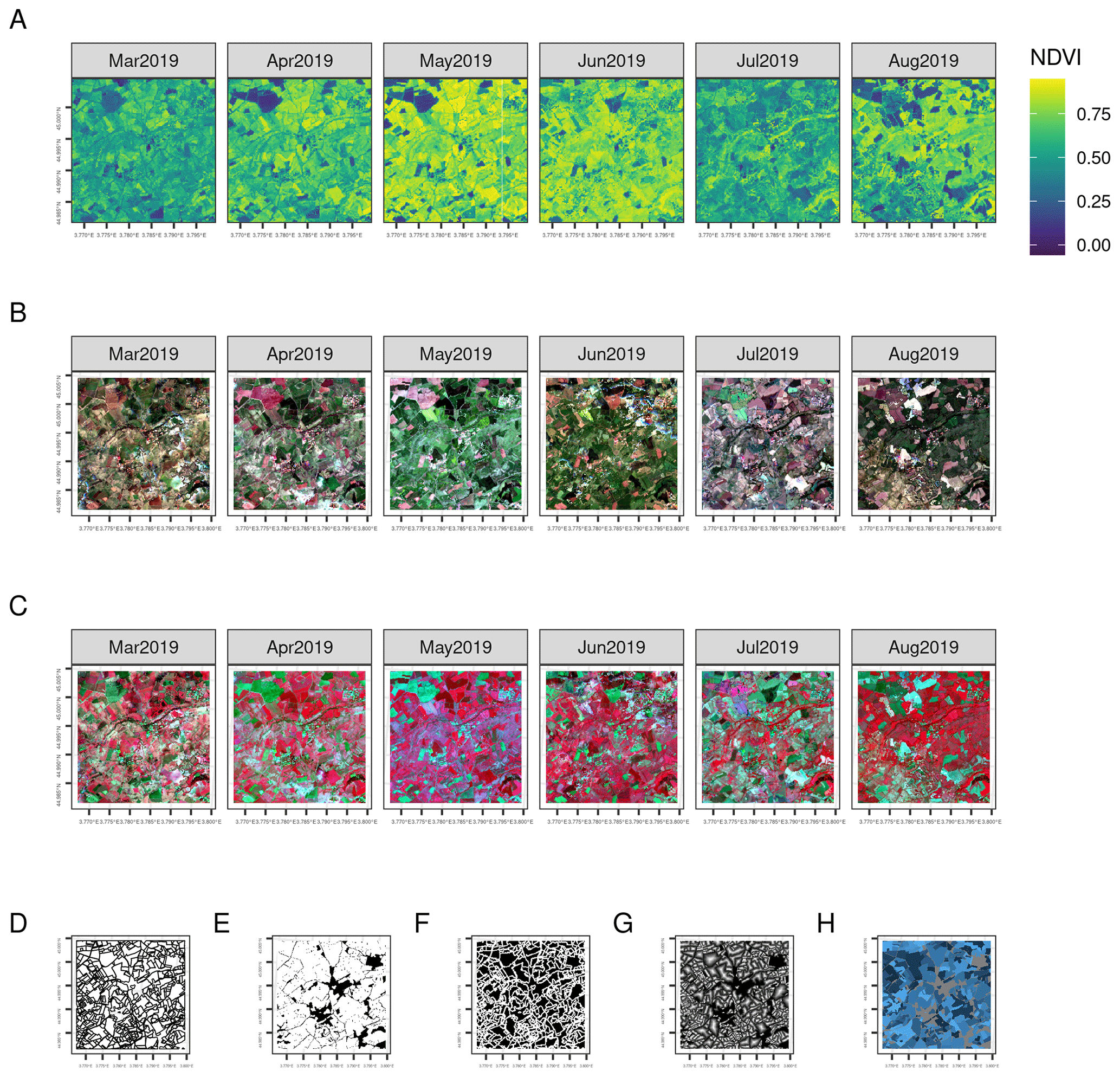
Figure 5Examples of the Sentinel-2 10 m dataset consisting of an extent of 256 pixels of 10 m (thus 2560 m by 2560 m). The samples are located in the South of France (sample ID 41781 with the extent coordinates 3827536, 2449682 to 3833405, 2453882 in EPSG 3035) . (a) NDVI monthly composite, (b) RGB monthly composites, and (c) NIR false colour monthly composites. The vector layer of the label is shown in (d). The label at the same resolution and extent consists of four layers: (e) an extent mask, (f) a boundary mask, (g) a distance mask, and (h) a field enumeration. See Fig. A3 for more detailed overview.

Figure 6Examples of the aerial orthophotos 1 m dataset consisting of an extent of 512 pixels of 1 m (thus 512 m by 512 m). (a) Aerial orthophoto RGB. The vector label (b) and the raster label at the same 1 m resolution and extent consist of four layers: (c) an extent mask, (d) a boundary mask, (e) a distance mask, and (f) a field enumeration.
2.2.2 Aerial orthophoto imagery
Orthophoto extraction was done using public Web Map Tile Service (WMTS) and Web Map Service (WMS) services for the seven regions (see details in Table A1). The orthophotos have a 1 m resolution and an extent of 512 by 512 pixels centred on the centroid of the sampled cells. After downloading a larger extent in the geographic reference system provided by the service, the samples are reprojected to EPSG 3035, cropped to the exact extent, and standardised on 3 RGB by removing the NIR band when available to have a consistent dataset. Finally, the histogram extraction of each sample has been used to filter out 233 of the 7831 samples (corresponding to 232 in Sweden and 1 in France), for which no data are available. Figure 7, along with the vector label data, shows random examples for each country.
The EU context in which aerial photography is collected is specific and has high requirements in terms of spatial accuracy. Indeed, in the EU, the aerial photography campaigns are driven by the need of administration to control the farmers' declarations' validity for aid application.The minimum accuracy requirement is defined in Article 70 of Regulation (EU) 1306/2013 as at least equivalent to that of cartography at a scale of 1:10 000 and, as from 2016, at a scale of 1:5000. This translates into (1) a horizontal absolute positional accuracy expressed as RMSE of 1.25 m (5000×0.25 mm = 1.25 m) (2) or the equivalent CE95 value, display range, and feature type content compatible with a map with a scale 1:5000 (i.e. topographic maps rather than urban survey maps), (3) using orthoimagery ≤ 0.5 m GSD (see more details in https://marswiki.jrc.ec.europa.eu/wikicap/index.php/Positional_Accuracy, last access: 11 January 2023).
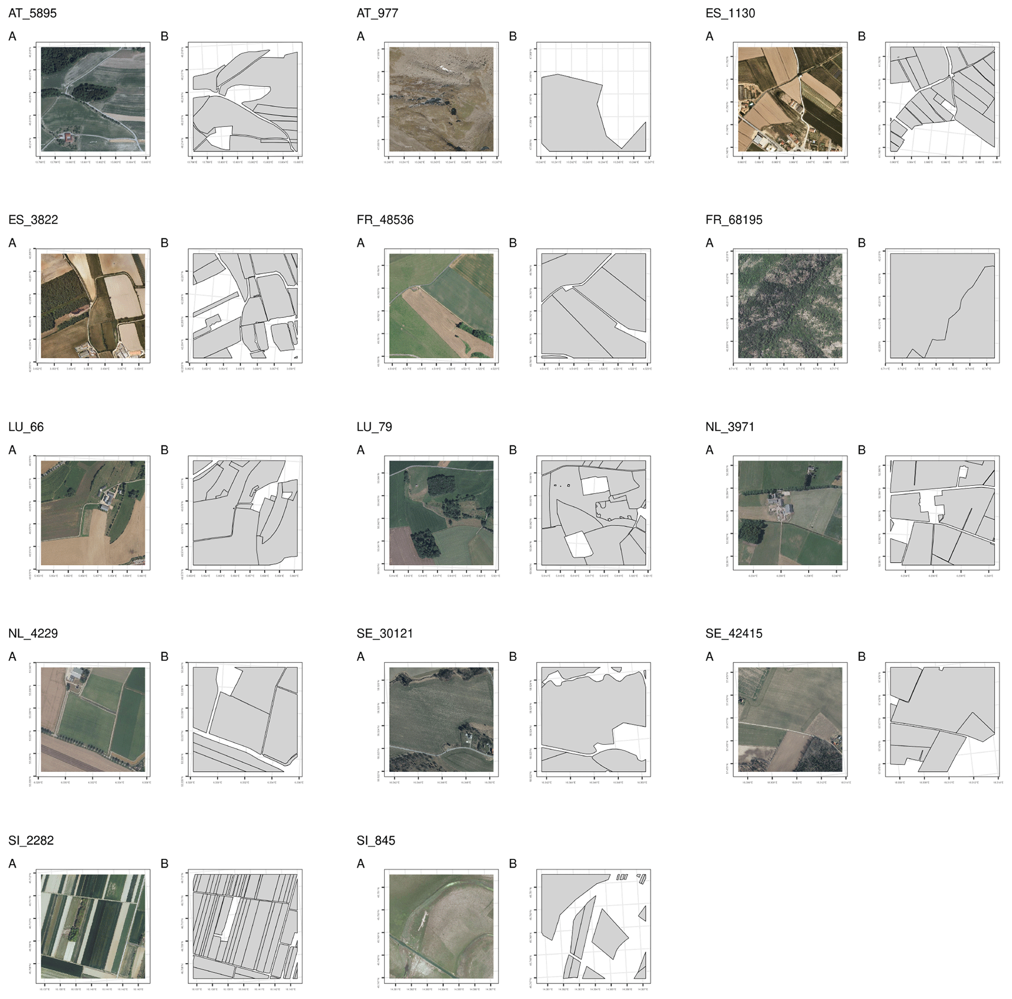
Figure 7Two random aerial orthophotos of (a) examples for each country along with the corresponding parcel vector labels (b). File ID including NUTS0 (e.g. AT_5895) is above each example.
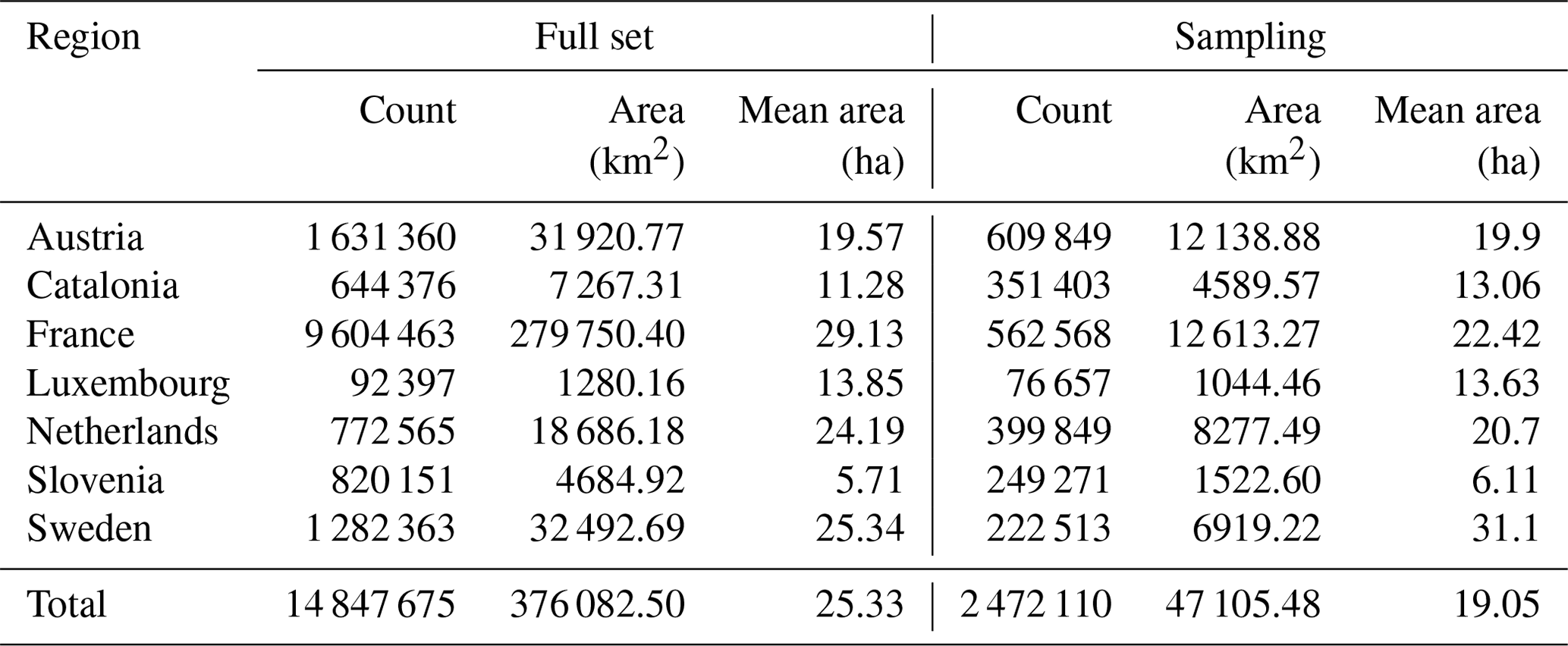
Table 2The original dataset contains 14.8 M parcels covering 376 K km2. The stratified sampling resulting in 7831 of 4 km samples contains 2.5 M parcels covering 47 105 km2. The mean area refers to parcel area in hectares, while the total mean area is here in the table the average area for the seven regions.
2.3 Label data
The labels are obtained from vector parcels of the GSAA for each specific region. The GSAA refers to the annual crop declarations made by EU farmers for CAP area-aid support measures. The electronic GSAA records include a spatial delineation of the parcels. A GSAA element is always a polygon of an agricultural parcel with one crop (or a single crop group with the same payment eligibility). The GSAA is operated at the region or country level in the EU-28, resulting in about 65 different designs and implementation schemes over the EU. Since these infrastructures are set up in each region, at the moment, data are not interoperable, nor are legends semantically harmonised. Furthermore, most GSAA data are not publicly available, although several countries are increasingly opening the data for public use. In this study, seven regions with publicly available GSAA are selected, representing a contrasting gradient across the EU. The Agri-food Data Portal from the Directorate General for Agriculture and Rural Development references Member State Geoportals, providing links where the data could be downloaded (https://agridata.ec.europa.eu/extensions/iacs/iacs.html, last access: 11 January 2023). After downloading the dataset, a reprojection to EPSG 3035 was done. From the original set of 14.8 M parcels covering 376 K km2 (Table 2), the 7831 of 4 km samples that contain 2.5 M parcels covering 47 105 km2 were selected. Finally, for both Sentinel-2 and orthophoto datasets, vector data were rasterised. The label is composed of four bands (example in Fig. 6b–e): vector label, boundary mask, distance mask, and field enumeration. See Fig. A3 for detailed overview of the label along with a Sentinel-2 RGB composite.
2.4 Train, validation, and test
We provide the orthophotos Zip archive with their respective masks to be used as a benchmark dataset (see Data availability section to access the data). The split between the samples respects a typical distribution, such as training of 70 %, validation of 15 %, and test of 15 %. The selection of the sampling is random. This information is stored in the column “split” of the CSV tables with the URLs of the files. As described previously, 233 samples, almost exclusively in Sweden, have no orthophotos available; thus, the split was done on 7598 files (7831 minus 233). The resulting random division provides 5319 files for training, 1140 for validation, 1139 for testing, and 233 as NA.
In this section, we point out some limitations and potential improvements of the approach and the proposed dataset.
The atmospheric corrections and cloud screening remain a challenge for Sentinel-2. We implemented a pragmatic approach to improve the bottom-of-atmosphere reflectance obtained from sen2cor (Main-Knorn et al., 2017). The Hampel outlier detection approach followed by a Savitsky–Golay smoothing allows to produce a 5 d interpolated smoothed data. However, residual cloud, cloud shadow, or haze thus jeopardise the development of applications (see Fig. A2 where undetected clouds result in artefacts on the time series). From the interpolated data, we obtain a median monthly composite to reduce the data size. This approach also has limitations and we could question the usefulness of interpolating the data if the ultimate goal is to produce a median monthly composite, as it could represent an extra computing burden with a limited added value.
In the regions covered by the dataset, the average size of the parcel is 25.33 ha, ranging from 5.71 ha in Slovenia to 29.13 ha in France. Sentinel-2 has also inherent limitations for small parcels monitoring as it was already highlighted (Vajsová et al., 2020). They show that about 10 % out of 867 fields less than 0.5 ha in size were not monitorable with Sentinel-2. Of course, parcel delineation is not the same, but it gives an idea on the limitations inherent to Sentinel-2 resolution. A good illustration to see the difference of the resolution between the Sentinel-2 and orthophoto data set is to look at the orthophoto on Fig. 6a and the same location cropped to the same extent on the Sentinel-2 in the Fig. A2.
The access to the orthophoto services was done either via WMTS or via WMS. A specific server access has to be used for each country with different projections (most in EPSG:3857, but some in local projections as shown in Table A1). While for most of the country, a specific capability layer allows to select the specific year of the service, the specific date of acquisition is most of the time unavailable. Additionally, the data quality is heterogeneous and depends on the specific acquisition.
The labels are obtained from GSAA containing inherent caveats. First of all, the geometry accuracy is referred to as , i.e. better than 1 m. Sometimes, parcels do not correspond to the agricultural field. Limitations of the labelled dataset could be the geometries, the timeliness, and also the semantics. As agricultural fields might be missing (e.g. due to not being present in original GSAA data), the data sets are really only suitable for the masked approach in training – the models trained on AI4Boundaries should only learn about the borders, extent, and distance of the included fields.
Several potential improvements have to be considered in the future.
First, in addition to the field boundaries, the crop type could be added to enable semantic segmentation similarly to Sykas et al. (2022). To do it properly over a large scale would require harmonising the legend of the GSAA from the different countries. A recent work (Schneider et al., 2021) has proposed a semantic harmonisation framework for this type of data and could thus serve as a basis.
Second, so far the AI4Boundaries data set covers only data sets from EU countries. To support the development of robust algorithm, the data set should be completed with a parcel from other geographical context. This is crucial to have validated and generalisable methods.
Another potential improvement would be to add other data sources such as radar data (e.g. Sentinel-1 coherence) or high-resolution satellite time series such as Planet data.
It is also very important to align such a type of data set with new emerging standards such as the one proposed by Radiant Earth ML HUB (https://mlhub.earth/, last access: 11 January 2023; Alemohammad, 2019). Their Spatio Temporal Asset Catalog (STAC) helps to make geospatial assets openly searchable and indexable.
A limitation of the proposed AI4Boundaries is its availability on an FTP server only, not directly callable as python packaged dataset. Having the data set accessible similarly to the Crop Harvest (Tseng et al., 2021) or Calisto (https://github.com/Agri-Hub/Callisto-Dataset-Collection, last access: 11 January 2023) would be more user-friendly.
Finally, the AI4Boundaries Sentinel-2 dataset has been used to train a model (based on the work of Waldner and Diakogiannis, 2020) that is available on Euro Data Cube (EDC) as an algorithm for on-demand automatic delineation of agricultural field boundaries over user-defined area of interest (AOI). The algorithm (https://collections.eurodatacube.com/field-delineation/, last access: 11 January 2023) uses Sentinel-Hub services for accessing Sentinel-2 data, and can be employed to produce baseline results for benchmarking purposes. In future work, the AI4Boundaries could be made available directly on EDC along with a tutorial on how to use it to increase the outreach to the community of potential users.
This section describes each data set provided along with this document and are downloadable at http://data.europa.eu/89h/0e79ce5d-e4c8-4721-8773-59a4acf2c9c9 (last access: 11 January 2023) (d'Andrimont et al., 2022):
-
./sampling.
ai4boundaries_sampling.gpkg. A geopackage vector file containing the 7831 4-by-4 km polygons of the sampling along with the stratification values as attributes.
ai4boundaries_ftp_urls_all.csv. A table that contains the path on the JRC FTP server of each Sentinel 2 tiles, orthophotos, and the respective labels of each. This also contains the split (i.e. train, test, val).
ai4boundaries_parcels_vector.gpkg. A vector file (geopackage) with the original parcel boundaries on the 4 km grid cell of the sampling.
-
./sentinel2.
./images. The folder contains seven folders – one for each NUTS0 region, amounting to a total of 7831 files named NUTS0_sampleID_S2_10m_256.nc. The files are NetCDF of Sentinel 2 tiles at 10 m ground resolution of 256 by 256 pixels and containing five bands (R, G, B, NIR, and NDVI) from March to August 2019.
./masks. The folder contains seven folders – one for each NUTS0 region, amounting to a total of 7831 files named NUTS0_sampleID_S2label_10m_256.tif. The files are Geotiff at 10 m ground resolution of 256 by 256 pixels and contain four bands.
ai4boundaries_ftp_urls_sentinel2_split.csv. This contains the URLs of the Sentinel-2 image and corresponding mask files along with the split (i.e. train, test, val).
-
./orthophoto.
./images. The folder contains seven folders - one for each NUTS0 region, amounting to a total of 7598 files named NUTS0_sampleID_ortho_1m_512.tif. The files are Geotiff at 1 m ground resolution of 512 by 512 pixels and contain three bands (R, G, B) acquired in 2019.
./masks. The folder contains seven folders – one for each NUTS0 region, amounting to a total of 7598 files named NUTS0_sampleID_ortholabel_1m_512.tif. The files are Geotiff at 1 m ground resolution of 512 by 512 pixels and contain four bands.
ai4boundaries_ftp_urls_orthophoto_split.csv. This contains the URLs of the orthophoto image and corresponding mask files along with the split (i.e. train, test, val).
A python-based library is also available to facilitate download: https://github.com/waldnerf/ai4boundaries (last access: 2 January 2023).
The AI4Boundaries data set provides a statistical sampling of agricultural parcel boundaries over key regions of Europe along with 10 m Sentinel-2 satellite time series and 1 m aerial orthophoto imagery. This unique data set allows to benchmark and compare parcel delineation methodologies in a transparent and reproducible way.
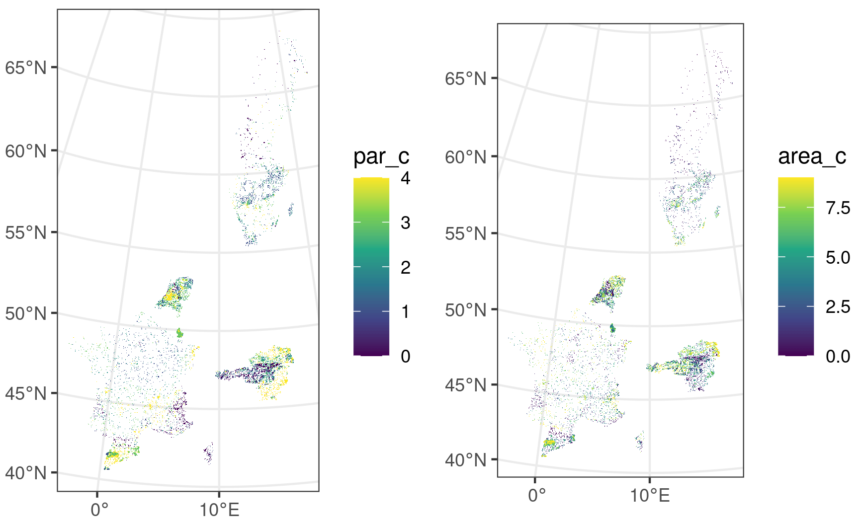
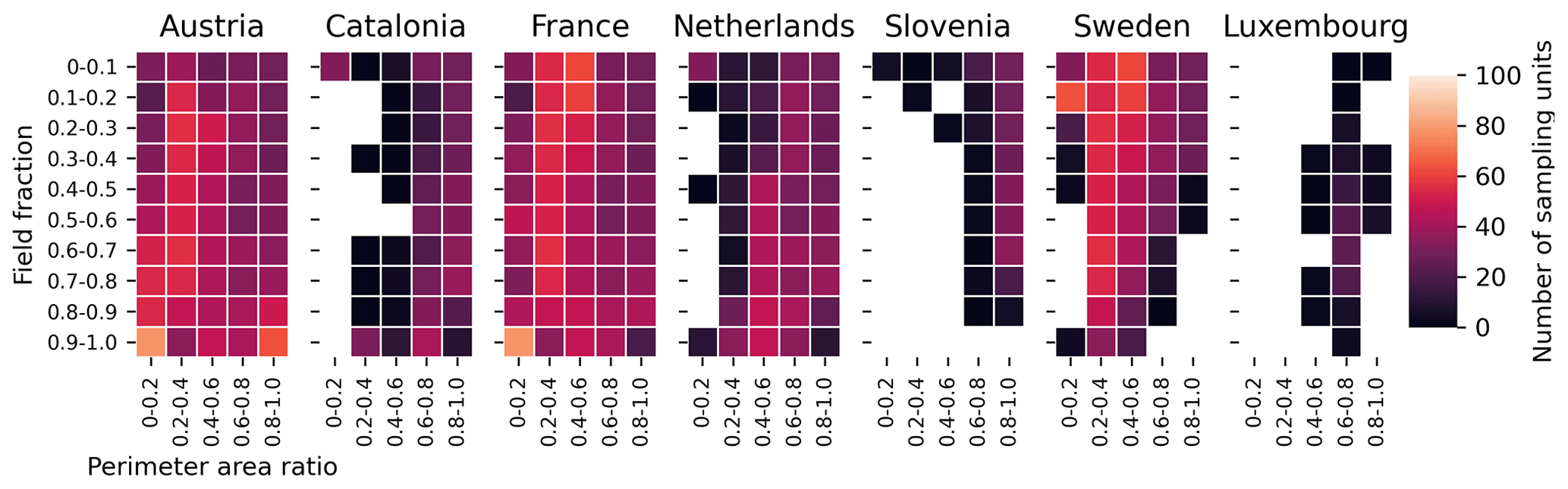
Figure A1Distribution of sampling units among the seven regions with the two variables used for the stratification.
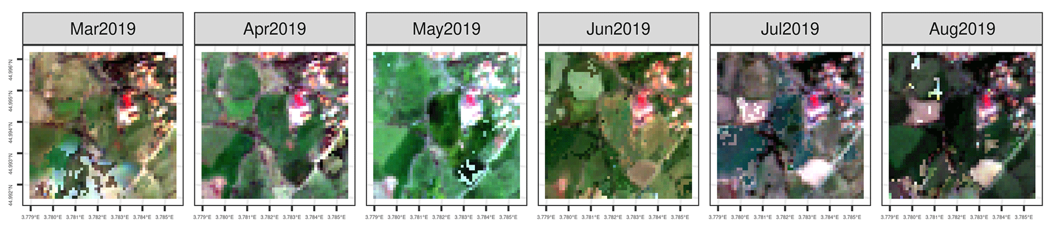
Figure A2Examples of the Sentinel-2 10 m cropped to an extent of the orthophoto data (thus 512 m by 512 m) for ease of comparison.
Table A1Aerial orthophoto WMTS and WMS services and projections.
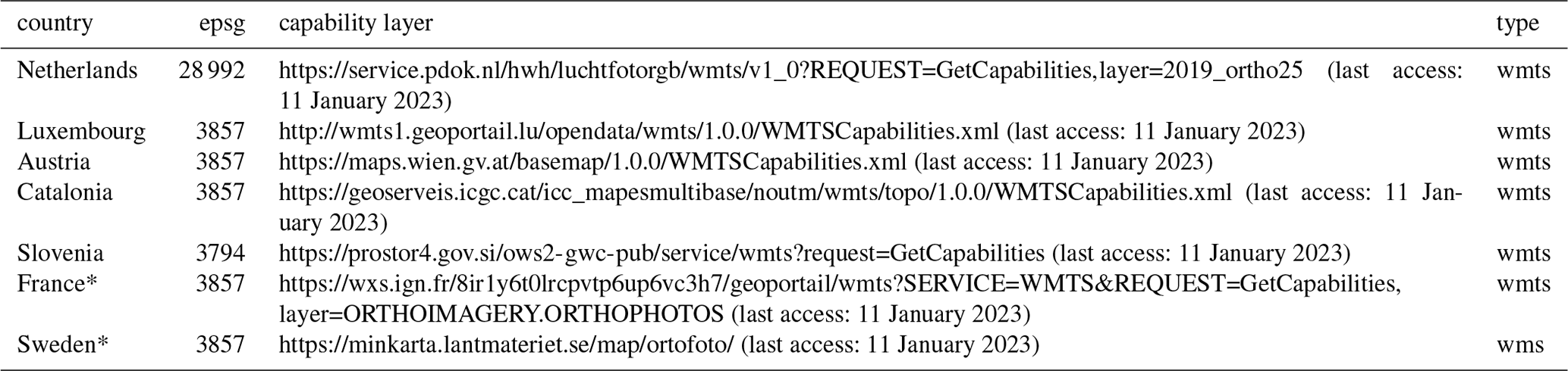
* Layers for France and Sweden require a password to download, which is available upon registration in the respective country's platform.
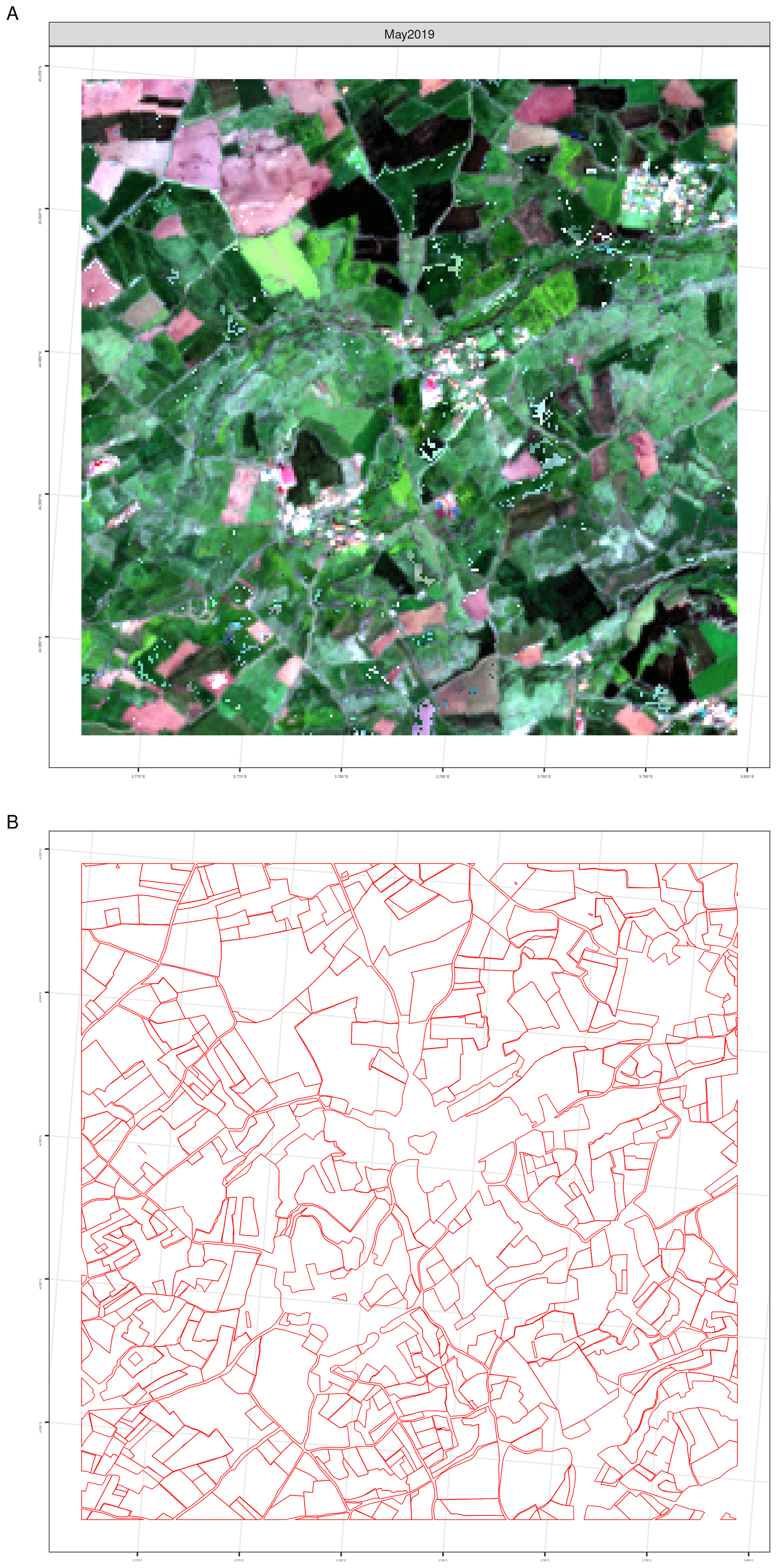
Figure A3Examples of the Sentinel-2 10 m data set consisting of an extent of 256 pixels of 10 m (thus, 2560 m by 2560 m). The samples are located in the South of France (sample ID 41781 with the extent coordinates 3827536, 2449682 to 3833405, 2453882 in EPSG 3035). (a) RGB May composites and (b) vector layer of the label.
Rd'A and FW conceptualised the study and designed the methodology. Rd'A, MC, PK, MY, DP, and FW processed the data. Rd'A, MC, PK, DM, MY, DP, and FW analysed the data and wrote the paper.
The contact author has declared that none of the authors has any competing interests.
Publisher's note: Copernicus Publications remains neutral with regard to jurisdictional claims in published maps and institutional affiliations.
The authors thank Ferdinando Urbano, Guido Lemoine, Marijn van der Velde, and Wim Devos for their support.
This paper was edited by Jia Yang and reviewed by two anonymous referees.
Alemohammad, H.: Radiant ML Hub [data set], https://www.radiant.earth/mlhub/ (last access: 11 January 2023), 2019. a
Aung, H. L., Uzkent, B., Burke, M., Lobell, D., and Ermon, S.: Farm parcel delineation using spatio-temporal convolutional networks, in: Proceedings of the IEEE/CVF Conference on Computer Vision and Pattern Recognition Workshops, 76–77, 2020. a
Brems, E., Lissens, G., and Veroustraete, F.: MC-FUME: A new method for compositing individual reflective channels, IEEE T. Geosci. Remote, 38, 553–569, https://doi.org/10.1109/36.823950, 2000. a
Chen, J., Jönsson, P., Tamura, M., Gu, Z., Matsushita, B., and Eklundh, L.: A simple method for reconstructing a high-quality NDVI time-series data set based on the Savitzky–Golay filter, Remote Sens. Environ., 91, 332–344, https://doi.org/10.1016/j.rse.2004.03.014, 2004. a
d'Andrimont, R., Claverie, M., Kempeneers, P., Muraro, D., Martinez Sanchez, L., and Waldner, F.: AI4boundaries, http://data.europa.eu/89h/0e79ce5d-e4c8-4721-8773-59a4acf2c9c9 [data set], 2022. a
European Commission, Joint Research Centre (JRC): AI4boundaries, European Commission, Joint Research Centre (JRC) [data set], http://data.europa.eu/89h/0e79ce5d-e4c8-4721-8773-59a4acf2c9c9, 2022. a
European Space Agency: ESA SNAP, http://step.esa.int, last access: 11 January 2023. a
Flood, N.: Seasonal Composite Landsat TM/ETM+ Images Using the Medoid (a Multi-Dimensional Median), Remote Sens., 5, 6481–6500, https://doi.org/10.3390/rs5126481, 2013. a
Garcia-Pedrero, A., Lillo-Saavedra, M., Rodriguez-Esparragon, D., and Gonzalo-Martin, C.: Deep learning for automatic outlining agricultural parcels: Exploiting the land parcel identification system, IEEE Access, 7, 158223–158236, 2019. a
Hampel, F. R.: The influence curve and its role in robust estimation, J. Am. Stat. A., 69, 383–393, 1974. a
Helber, P., Bischke, B., Dengel, A., and Borth, D.: EuroSAT: A novel dataset and deep learning benchmark for land use and land cover classification, IEEE J. Sel. Top. Appl. Earth Obs., 12, 2217–2226, 2019. a
Kempeneers, P., Pesek, O., De Marchi, D., and Soille, P.: pyjeo: A Python Package for the Analysis of Geospatial Data, ISPRS International Journal of Geo-Information, 8, 461, https://doi.org/10.3390/ijgi8100461, 2019. a
Main-Knorn, M., Pflug, B., Louis, J., Debaecker, V., Müller-Wilm, U., and Gascon, F.: Sen2Cor for sentinel-2, in: Image and Signal Processing for Remote Sensing XXIII, SPIE, 10427, 37–48, 2017. a, b
Masoud, K. M., Persello, C., and Tolpekin, V. A.: Delineation of agricultural field boundaries from Sentinel-2 images using a novel super-resolution contour detector based on fully convolutional networks, Remote Sens., 12, 59, https://doi.org/10.3390/rs12010059, 2019. a
Potapov, P., Turubanova, S., and Hansen, M. C.: Regional-scale boreal forest cover and change mapping using Landsat data composites for European Russia, Remote Sens. Environ., 115, 548–561, https://doi.org/10.1016/j.rse.2010.10.001, 2011. a
Rußwurm, M., Pelletier, C., Zollner, M., Lefèvre, S., and Körner, M.: Breizhcrops: A time series dataset for crop type mapping, arXiv preprint, arXiv:1905.11893, 2019. a
Schneider, M., Broszeit, A., and Körner, M.: Eurocrops: A pan-european dataset for time series crop type classification, arXiv preprint, arXiv:2106.08151, 2021. a
Soille, P., Burger, A., De Marchi, D., Kempeneers, P., Rodriguez, D., Syrris, V., and Vasilev, V.: A versatile data-intensive computing platform for information retrieval from big geospatial data, Future Gener. Comp. Sy., 81, 30–40, 2018. a
Sumbul, G., Charfuelan, M., Demir, B., and Markl, V.: Bigearthnet: A large-scale benchmark archive for remote sensing image understanding, in: IGARSS 2019–2019 IEEE International Geoscience and Remote Sensing Symposium, IEEE, 5901–5904, 2019. a
Sykas, D., Sdraka, M., Zografakis, D., and Papoutsis, I.: A Sentinel-2 multi-year, multi-country benchmark dataset for crop classification and segmentation with deep learning, arXiv, https://doi.org/10.48550/ARXIV.2204.00951, 2022. a, b
Tarasiou, M., Güler, R. A., and Zafeiriou, S.: Context-self contrastive pretraining for crop type semantic segmentation, IEEE T. Geosci. Remote, 60, 1–7, 2021. a
Tseng, G., Zvonkov, I., Nakalembe, C. L., and Kerner, H.: CropHarvest: A global dataset for crop-type classification, in: Thirty-fifth Conference on Neural Information Processing Systems Datasets and Benchmarks Track (Round 2), https://github.com/nasaharvest/cropharvest (last access: 12 January 2023), 2021. a
Tuvdendorj, B., Zeng, H., Wu, B., Elnashar, A., Zhang, M., Tian, F., Nabil, M., Nanzad, L., Bulkhbai, A., and Natsagdorj, N.: Performance and the Optimal Integration of Sentinel-1/2 Time-Series Features for Crop Classification in Northern Mongolia, Remote Sens., 14, 1830, https://doi.org/10.3390/rs14081830, 2022. a
Vajsová, B., Fasbender, D., Wirnhardt, C., Lemajic, S., and Devos, W.: Assessing spatial limits of Sentinel-2 data on arable crops in the context of checks by monitoring, Remote Sens., 12, 2195, https://doi.org/10.3390/rs12142195, 2020. a
Waldner, F. and Diakogiannis, F. I.: Deep learning on edge: Extracting field boundaries from satellite images with a convolutional neural network, Remote Sens. Environ., 245, 111741, https://doi.org/10.1016/j.rse.2020.111741, 2020. a, b, c
Waldner, F., Diakogiannis, F. I., Batchelor, K., Ciccotosto-Camp, M., Cooper-Williams, E., Herrmann, C., Mata, G., and Toovey, A.: Detect, consolidate, delineate: Scalable mapping of field boundaries using satellite images, Remote Sens., 13, 2197, https://doi.org/10.3390/rs13112197, 2021. a
Wang, S., Waldner, F., and Lobell, D. B.: Unlocking Large-Scale Crop Field Delineation in Smallholder Farming Systems with Transfer Learning and Weak Supervision, Remote Sens., 14, 5738, https://doi.org/10.3390/rs14225738, 2022. a