the Creative Commons Attribution 4.0 License.
the Creative Commons Attribution 4.0 License.
 | 28 Jun 2023
The EUPPBench postprocessing benchmark dataset v1.0
Jonathan Demaeyer
Jonas Bhend
Sebastian Lerch
Cristina Primo
Bert Van Schaeybroeck
Aitor Atencia
Zied Ben Bouallègue
Jieyu Chen
Markus Dabernig
Gavin Evans
Jana Faganeli Pucer
Ben Hooper
Nina Horat
David Jobst
Janko Merše
Peter Mlakar
Annette Möller
Olivier Mestre
Maxime Taillardat
Stéphane Vannitsem
Statistical postprocessing of medium-range weather forecasts is an important component of modern forecasting systems. Since the beginning of modern data science, numerous new postprocessing methods have been proposed, complementing an already very diverse field. However, one of the questions that frequently arises when considering different methods in the framework of implementing operational postprocessing is the relative performance of the methods for a given specific task. It is particularly challenging to find or construct a common comprehensive dataset that can be used to perform such comparisons. Here, we introduce the first version of EUPPBench (EUMETNET postprocessing benchmark), a dataset of time-aligned forecasts and observations, with the aim to facilitate and standardize this process. This dataset is publicly available at https://github.com/EUPP-benchmark/climetlab-eumetnet-postprocessing-benchmark (31 December 2022) and on Zenodo (https://doi.org/10.5281/zenodo.7429236, Demaeyer, 2022b and https://doi.org/10.5281/zenodo.7708362, Bhend et al., 2023). We provide examples showing how to download and use the data, we propose a set of evaluation methods, and we perform a first benchmark of several methods for the correction of 2 m temperature forecasts.
- Article
(4311 KB) - Full-text XML
-
Supplement
(1201 KB) - BibTeX
- EndNote


Since the advent of numerical weather prediction, statistical postprocessing techniques have been used to correct forecast biases and errors. The term “postprocessing techniques” here refers to methods which use past forecasts and observations to learn information about forecast deficiencies that can then be used to correct future forecasts. Nowadays, postprocessing of weather forecasts is an important part of the forecasting chain in modern prediction systems at national and international meteorological services.
Many postprocessing approaches have been proposed during the last half century, ranging from the so-called perfect prog method (Klein et al., 1959; Klein and Lewis, 1970) to Bayesian model averaging (BMA) techniques (Raftery et al., 2005) and including the emblematic model output statistics (MOS) approach (Glahn and Lowry, 1972). Some of these methods have been adapted to deal with ensemble forecasts and also calibrate the associated forecast probabilities, like the ensemble MOS (EMOS) method (Gneiting et al., 2005). Recently, machine learning-based methods have been proposed (Taillardat et al., 2016; Rasp and Lerch, 2018; Bremnes, 2020), which were shown to improve upon the conventional methods (Schulz and Lerch, 2022).
Systematic intercomparison exercises of both univariate (e.g., Rasp and Lerch, 2018; Schulz and Lerch, 2022; Chapman et al., 2022) and multivariate (e.g., Wilks, 2015; Perrone et al., 2020; Lerch et al., 2020; Chen et al., 2022; Lakatos et al., 2023) postprocessing methods exist, often based on artificial simulated datasets mimicking properties of real-world ensemble forecasting systems or based on real-world datasets consisting of ensemble forecasts and observations for specific use cases. However, there is no comprehensive, widely applicable benchmark dataset available for station- and grid-based postprocessing that facilitates reuse and comparisons, including a large set of potential input predictors and several target variables relevant to operational weather forecasting at meteorological services. The aim of the present work is to pave the way towards achieving these aims, with the publication of an extensive – analysis-ready – forecast and observation dataset, consisting of both gridded data and data at station locations. By an analysis-ready dataset, we mean that the dataset formatting is tailored to obtain the most optimal match between observations and forecasts. In practice, this means that the observations are not provided as conventional time series but rather at the times and locations that match the forecasts.
Recently, the need for a common platform based on which different postprocessing techniques of weather forecasts can be compared was highlighted (Vannitsem et al., 2021) and extensively discussed between several members of the expert team of the postprocessing module running within the programs of the European Meteorological Network (EUMETNET). Here, we introduce the first step in the development of such a platform, in the form of an easily accessible dataset that can be used by a large community of users interested in the design of efficient postprocessing algorithms of weather forecasts for different applications. As stated in Dueben et al. (2022), comprehensive benchmark datasets are needed to enable a fair, quantitative comparison between different tools and methods while reducing the need to design and build them, a task which requires domain-specific knowledge. In this view, common benchmark datasets facilitate the collaboration of different communities with different expertise, by lowering the energy barrier required to embark on specific problems which would have otherwise required an excessive and discouraging amount of resources.
Many datasets related to weather and climate prediction were released during the last 3 years, emphasizing the need and appetite of the field for ever more data. For instance, datasets have been published related to sea ice drift (Rabault et al., 2022), to hydrology (Han et al., 2022), to learning of cloud classes (Zantedeschi et al., 2019), to subseasonal and seasonal weather forecasting (Rasp et al., 2020; Garg et al., 2022; Lenkoski et al., 2022; Wang et al., 2022), to data-driven climate projections (Watson-Parris et al., 2022), and – most relevant to the present work – to the benchmarking of postprocessing methods (Haupt et al., 2021; Ashkboos et al., 2022; Kim et al., 2022). Haupt et al. (2021) distribute a collection of (partly preexisting) different datasets for specific postprocessing tasks, including ensemble forecasts of the Madden–Julian Oscillation, integrated vapor transport over the eastern Pacific and western United States, temperature over Germany, and surface road conditions in the United Kingdom. By contrast, Ashkboos et al. (2022) provide a reduced set of global gridded 10-member ECMWF ensemble forecasts for selected target variables.
Providing weather- or climate-related datasets to the scientific community in a standardized and persistent way remains a challenge, which was recently simplified by the introduction of efficient tools to store and provide data to the users. We can mention, for example, xarray (Hoyer and Joseph, 2017), Zarr (Miles et al., 2020), dask (https://github.com/dask/dask, last access: 24 April 2023) and the package climetlab (https://github.com/ecmwf/climetlab, last access: 24 April 2023), recently developed by the European Centre for Medium-Range Weather Forecasts (ECMWF). The dataset introduced in the present article is, for instance, provided by a climetlab plugin (https://github.com/EUPP-benchmark/climetlab-eumetnet-postprocessing-benchmark, last access: 24 April 2023) but also accessible through other means and programming languages (see the Supplement).
The EUPPBench (EUMETNET postprocessing benchmark) dataset consists of gridded and point ECMWF subdaily forecasts of different kinds (deterministic high-resolution, ensemble forecasts and reforecasts) over central Europe (see Fig. 1). EUPPBench encompasses both station- and grid-based forecasts for many different variables, enabling a large variety of applications. This – complemented by the inclusion of reforecasts – enables a realistic representation of operational postprocessing situations, allowing users and institutions to learn and improve their skills on this crucial process. These operational aspects are, to our knowledge, missing in the currently available postprocessing benchmark datasets.
The forecasts and reforecasts of EUPPBench are paired with station observations and gridded reanalysis for the purpose of training and verifying postprocessing methods. To demonstrate how this dataset can be used, a benchmark of state-of-the-art postprocessing methods has been conducted to improve medium-range temperature forecasts. Although limited in scope, the outcome of this benchmark already emphasizes the potential of the dataset to provide meaningful results and provides useful insights into the potential, diversity and limitations of postprocessing over the study domain. Additionally, performing the benchmark for the first time with a large community also allows us to address the usefulness of the established guidelines and protocols and to draw conclusions, which are important assets for the delivery of many more benchmarks to come.
This article is structured as follow. The dataset structure and metadata are introduced in Sect. 2. The design and the verification setup of the benchmark which was carried out upon publication of this dataset is explained in Sect. 3, while in Sect. 4 the benchmarked methods are detailed. The results of the benchmark are presented in Sect. 5. We draw some interesting conclusions in Sect. 7 and outline plans for the future development of the dataset and of other benchmarks to come. Finally, the code of the benchmark and the data availability of the dataset are provided in Sect. 6.
The EUPPBench dataset is available on a portion of Europe covering 45.75 to 53.5∘ in latitude and 2.5 to 10.5∘ in longitude. Therefore, this domain includes mainly Belgium, France, Germany, Switzerland, Austria and the Netherlands. It is stored in Zarr format, a CF-compatible format (https://cfconventions.org/, last access: 24 April 2023) (Gregory, 2003; Eaton et al., 2003), which provides easy access and allows users to “slice” the data along various dimensions in an effortless and efficient manner. In addition, the forecast and observation data are already paired together along corresponding dimensions, therefore providing an analysis-ready dataset for postprocessing benchmarking purposes.
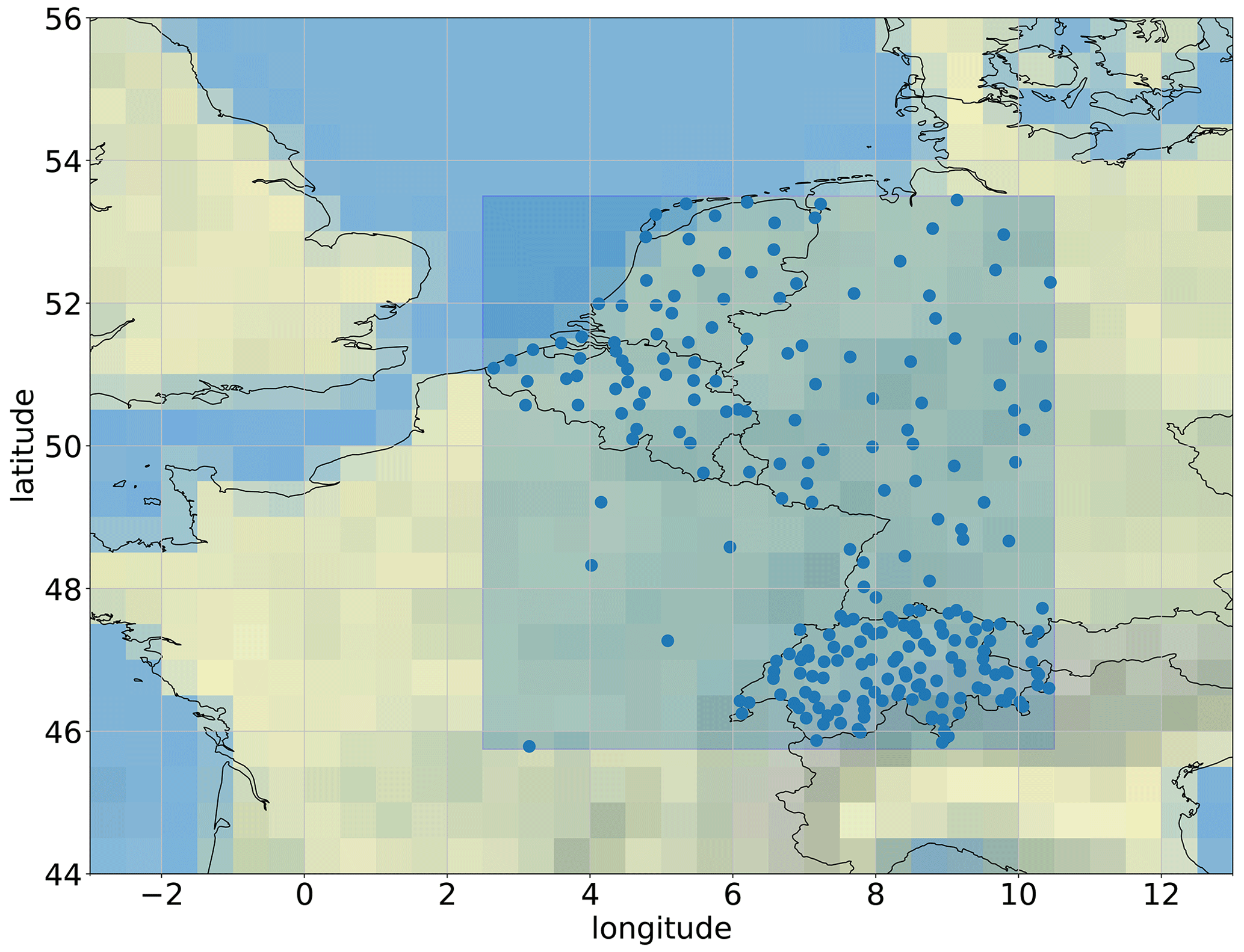
Figure 1Spatial coverage of the dataset. Blue rectangle: spatial domain of the gridded dataset. Blue dots: position of the stations included in the dataset. Grey lines depict the latitude and longitude grid.
EUPPBench includes both the 00:00 Z (midnight) subdaily ensemble forecasts and reforecasts (Hagedorn et al., 2008; Hamill et al., 2008) produced by the Integrated Forecasting System (IFS) of ECMWF during the years 2017 and 2018, which are released by the forecasting center under the CC-BY-4.0 license. Therefore, there are 730 forecast dates and 209 reforecast dates over the 2-year span, with reforecasts being produced twice a week (Monday and Thursday). Apart from the ensemble forecasts and reforecasts, the high-resolution deterministic forecasts are also included. Each reforecast date, however, consists of 20 past forecasts computed with the model version valid at the reforecast date and initialized from 1 to 20 years in the past at the same date of the year, thereby covering the period 1997–2017. In total, there are 4180 reforecasts. The numbers of ensemble members are 51 and 11 for the forecasts and reforecasts, respectively. This includes the forecast control run which is assumed to have the closest initial conditions to reality. The choice of the years 2017 and 2018 was motivated by the relatively small number of model changes in the ECMWF forecast system during that period and, most importantly, the absence of model resolution modifications, as shown by Table 1. This implementation constraint is crucial to ensure that no supplementary model error biases are introduced in the datasets, as those biases can lead to a more-or-less severe degradation of the postprocessing performances (Lang et al., 2020; Demaeyer and Vannitsem, 2020).
Table 1ECMWF IFS model changes during the 2017–2018 time span.
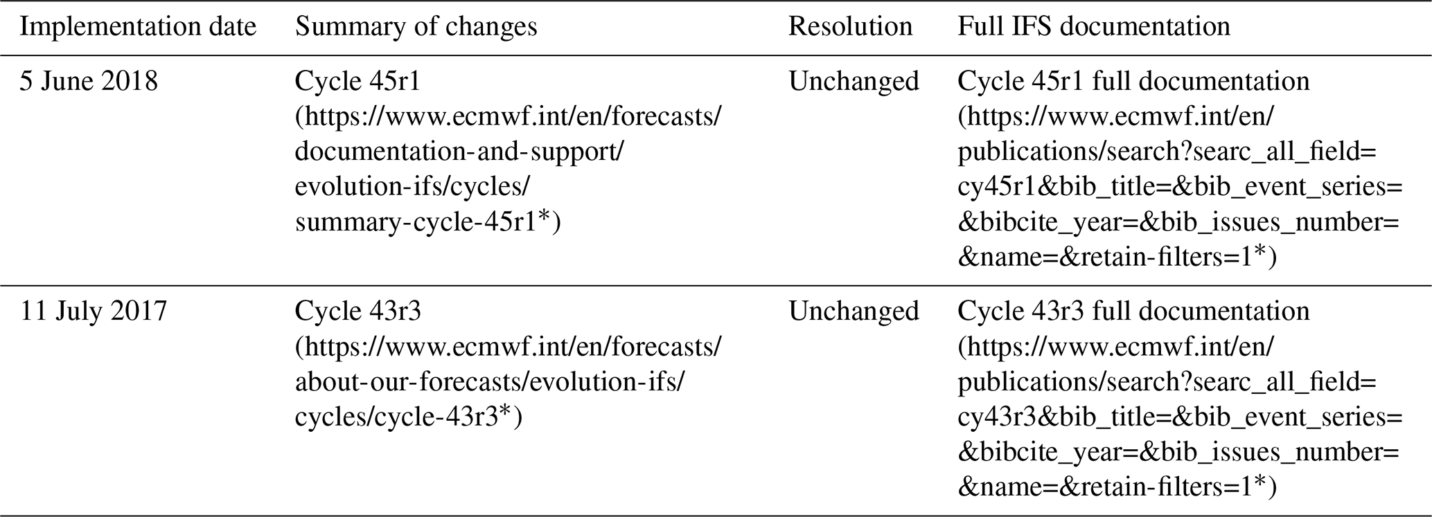
Source: https://www.ecmwf.int/en/forecasts/documentation-and-support/changes-ecmwf-model (last access: 2 December 2022). * Last access: 2 June 2023.
The forecast and reforecast time steps are 6-hourly (including the 0th analysis time steps) up to a lead time of 120 h (5 d). The variables considered are mainly surface variables and can be classified into two main categories: instantaneous or processed. Table 2 details these two different kinds of variable. Here, a “processed variable” means that the corresponding variable has either been accumulated, averaged or filtered over the past 6 h. In addition to these surface variables, the extreme forecast indices1 (Lalaurette, 2003; Zsótér, 2006) and some pressure-level variables are also available (see Tables 3 and 4, respectively).
Table 2List of instantaneous and processed forecast variables on the surface level available in EUPPBench, all available in the EUPPBench gridded and station-location forecast datasets, and the availability of the corresponding gridded and station-location observations. The presence (“yes”) or absence (“no”) of corresponding observations are shown in the last two columns.
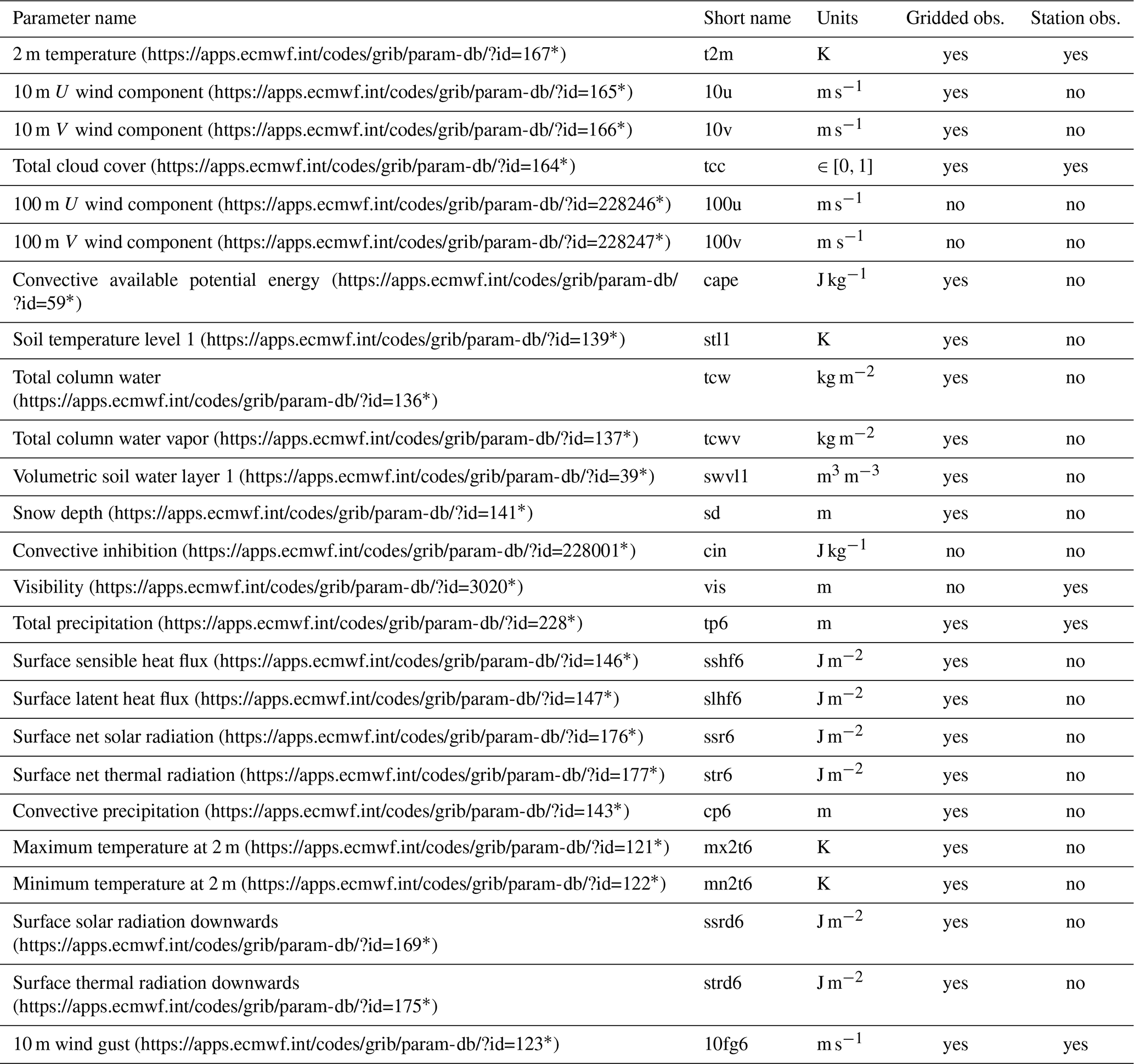
Remark: a “6” was added to the usual ECMWF short names to indicate the span (in hours) of the accumulation or filtering. * Last access: 22 December 2022.
Table 3List of available extreme forecast indices, all available in the EUPPBench gridded and station-location forecast datasets.
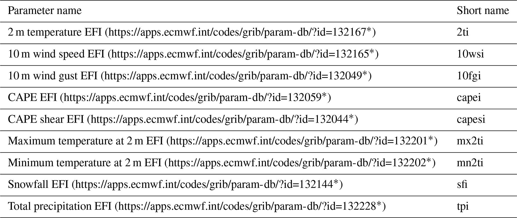
Remark: by definition, observations are not available for the EFI. The EFIs are available for the model step ranges (in hours) 0–24, 24–48, 48–72, 72–96, 96–120, 120–144 and 144–168. The range of values of EFI goes from −1 to +1. * Last access: 22 December 2022.
Table 4List of variables on pressure levels, all available in the EUPPBench gridded and station-location forecast datasets.
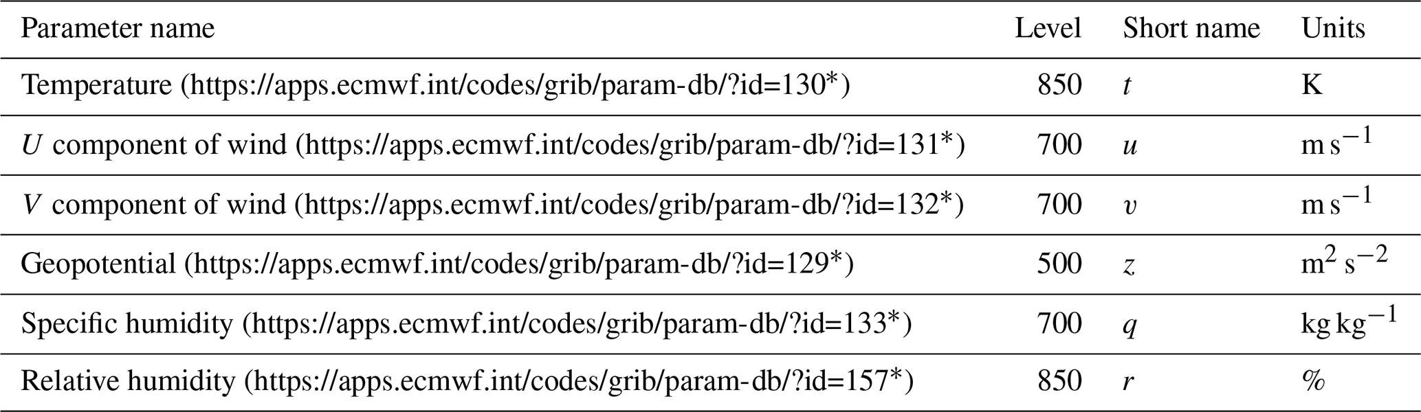
Remark: only gridded observations (reanalysis) are available for these variables. * Last access: 22 December 2022.
2.1 General data structure
The EUPPBench dataset consists of observations and forecasts in two types: a gridded dataset and a dataset at station locations. All forecasts are based on the ECMWF IFS forecasts. However, while the observational dataset at the station locations is based on ground measurements, the reanalysis ERA5 is taken as the gridded observational dataset. All forecast and reforecast datasets are provided for 31 variables, and additionally, the forecast dataset includes 9 EFI variables. The observations, on the other hand, include only 5 and 21 variables for the station-location and gridded datasets, respectively. Additionally metadata on the model and observations are provided.
How to access the datasets is documented in the Sect. 6. We now detail in the following subsections the sources and properties of both dataset formats.
2.2 Gridded data
All gridded EUPPBench data are provided on a regular grid of 0.25∘ × 0.25∘, corresponding roughly to a 25 km horizontal resolution at midlatitudes. As mentioned before, the forecasts and reforecasts are provided by the ECMWF forecasting model in operation at the moment of their issuance. They have both been regridded from the ECMWF original ensemble forecasts O640 (or O1280 for the deterministic forecasts)2 grid to the regular grid using the ECMWF MIR interpolation package (Maciel et al., 2017), provided automatically by the MARS archive system. This regridding was done to be in line with the resolution of the ERA5 reanalysis (Hersbach et al., 2020), which provides the gridded observations of the EUPPBench dataset.
We recognize that gridded observational datasets over the study domain exist for specific variables that are more accurate than ERA5. For instance, in the case of precipitation-related variables (like the total precipitation contained in the dataset at hand), ERA5 has been shown to provide – compared to other datasets – a poor agreement with station observations (Zandler et al., 2019), mixed performances when used to derive hydrological products (Hafizi and Sorman, 2022), yet good results when using perfect prog downscaling methods (Horton, 2022). Notwithstanding, we emphasize that the goal of this gridded dataset is to provide a representative “truth” for the purpose of benchmarking of postprocessing methods. Additionally, the availability of a wide range of variables in ERA5 and the spatiotemporal consistency among different meteorological variables (a very important aspect in the present context) cannot be provided by gridded observational datasets.
2.3 EUPPBench data at station locations
Subdaily station observations have been provided by many national meteorological services (NMSs) participating in the construction of this dataset, and a big part of the station data can be considered open data (see Sect. 6). The observations of 234 stations cover the entire 22-year time period 1997–2018 necessary to match the reforecasts and forecasts. The elevation of these stations varies from a few meters below the sea level up to 3562 m for the Jungfraujoch station in Switzerland. These stations constitute the most authoritative sources of information about weather and climate provided in each of the involved countries, being constantly monitored and having the quality of the data checked.
The EUPPBench dataset at station locations consists of the ECMWF forecasts and reforecasts at the grid point closest to the station locations and the associated observations, matched for each lead time. As shown in Table 2, there are five variables currently available: 2 m temperature (t2m), total cloud cover (tcc), visibility (vis), total precipitation (tp6) and 10 m wind gust (10fg6). More observation variables will be added in subsequent versions of the dataset.
2.4 Static data and metadata
In addition to the forecasts and reforecasts, auxiliary fields are provided, such as the land usage and the surface geopotential which is proportional to the model orography (see Fig. 2). Table 5 synthesizes this part of the dataset. These constant fields have been extracted and are also provided in the station metadata.
Table 5List of available constant fields.
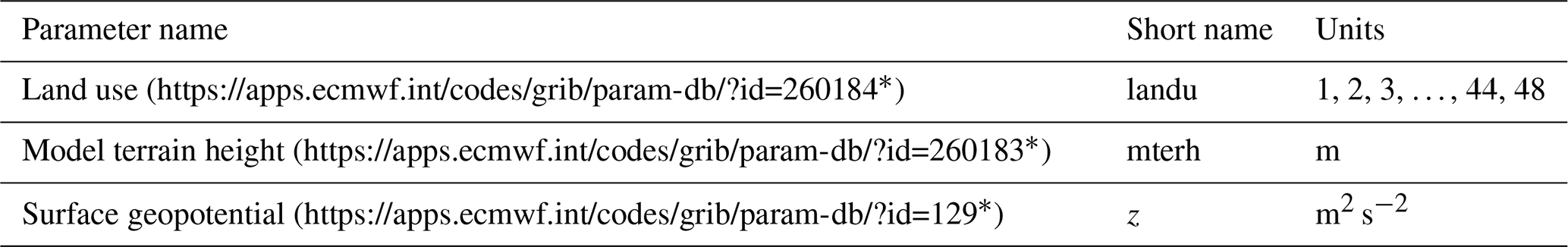
The land usage is extracted from the CORINE2018 (https://land.copernicus.eu/pan-european/corine-land-cover, last access: 30 July 2022) dataset (Copernicus Land Monitoring Service, 2018). More details are provided in the legend entry of the metadata within each file. The model terrain height is extracted from the EU-DEM v1.1 (https://land.copernicus.eu/imagery-in-situ/eu-dem, last access: 1 August 2023) data elevation model dataset (Copernicus Land Monitoring Service, 2022). Finally, the model orography can be obtained by dividing the surface geopotential by g=9.80665 m s−2. * Last access: 22 December 2022.
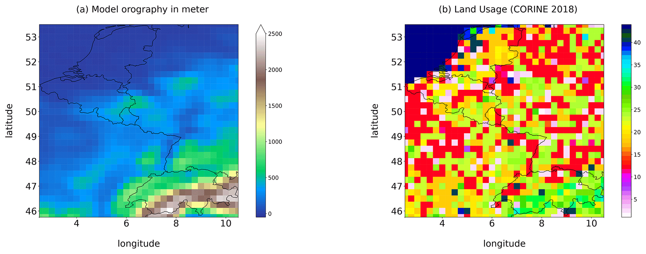
Figure 2Static fields in the gridded dataset. (a) The model orography obtained by dividing the model surface geopotential by g=9.80665 m s−2. (b) Grid point land usage provided by the CORINE 2018 dataset (Copernicus Land Monitoring Service, 2018). Numerical codes indicating the usage categories are included in the dataset metadata.
Depending on the kind of dataset, dimensions and different information are embedded in the data. For gridded data, the metadata available in the forecast, reforecast and observation datasets are detailed in Table 6. For station data, the forecast and reforecast metadata are detailed in Table 7, while the observation metadata are detailed in Table 8. For all data, attributes specifying the sources and the license are always provided.
Table 6The metadata provided in the files of the gridded forecasts, reforecasts and observational datasets.
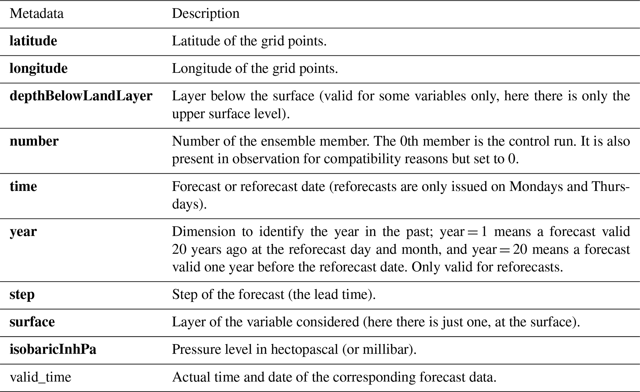
Remark: bold metadata denote dimensions indexing the datasets.
Table 7The metadata provided in the files of the forecast, reforecast at the station locations.
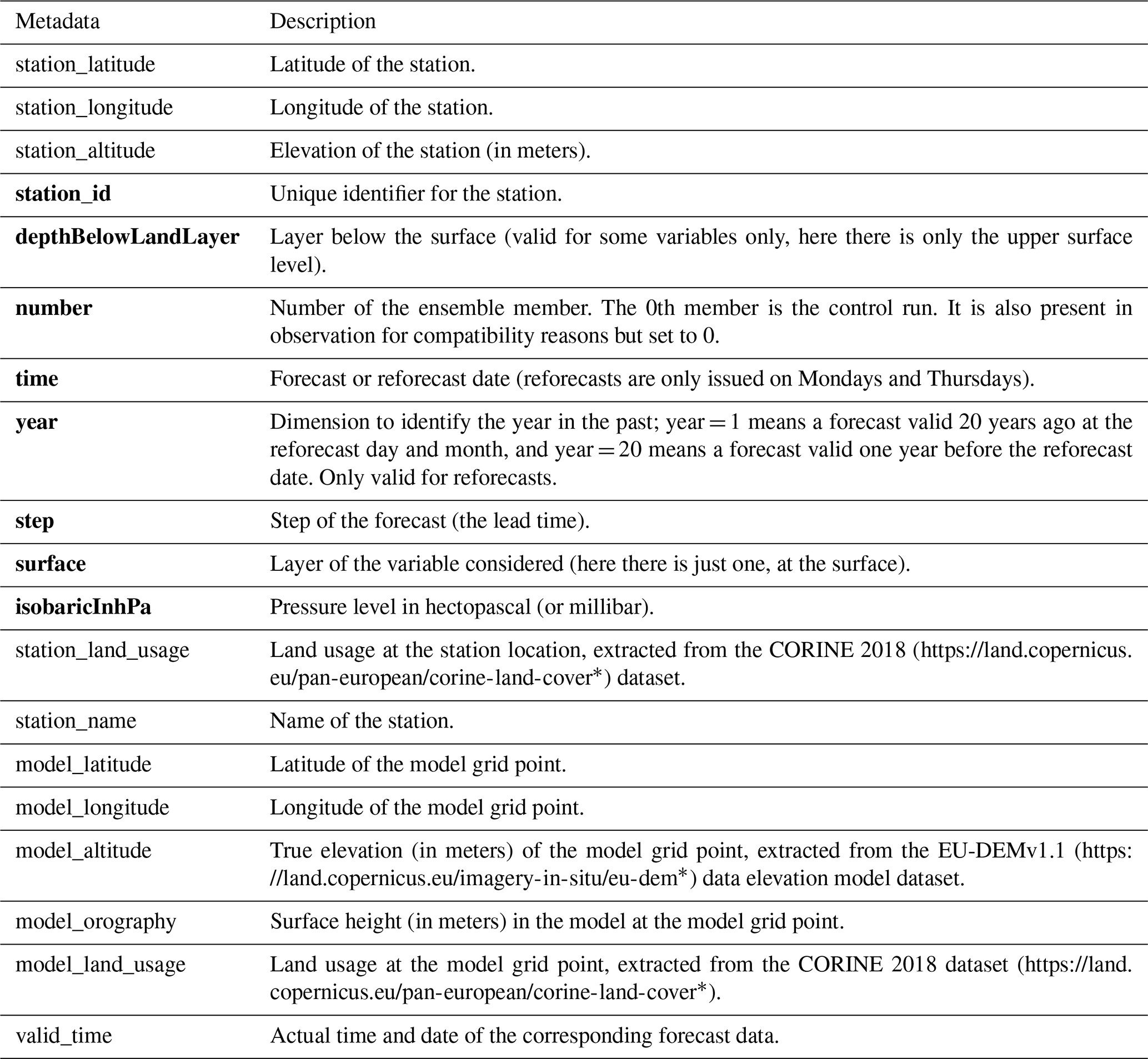
Remark 1: bold metadata denote dimensions indexing the datasets. Remark 2: the metadata with “model” in their name indicate properties of the closest model grid point to the station location, and at which the forecasts corresponding to the station observations was extracted from the gridded dataset. * Last access: 1 August 2022.
Table 8Station observations metadata
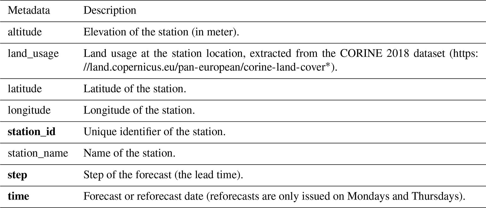
Remark: bold metadata denote dimensions indexing the datasets. * Last access: 30 June 2022.
To illustrate the usefulness of the EUPPBench dataset, a benchmark of several state-of-the-art postprocessing methods – many of which are currently in operation in NMSs – was performed, including some more recent and more advanced methods. This first exercise was based on a small subset of the dataset. Along the same line, the verification process of this benchmark also focused on some general aspects typically considered for operational postprocessing. In this section, we describe the general framework that we used to conduct this benchmark. The following sections will be devoted to the methods and the results obtained. We begin by detailing the design of this experiment.
3.1 Experiment design
The postprocessing benchmark at hand considers the correction of the ensemble forecasts of the 2 m temperature at the nearest forecast grid point from every station available in the dataset, spanning several European countries and the whole EUPPBench area. We note that this area includes orographically difficult regions, nearly flat plains, and also stations close to the sea or located on islands. Discrepancies may therefore occur between forecasts and observations due to poor observational representativity at the scale of the model or due to challenges in the model representation of a wide range of physical processes. We note also that, due to the coarse nature of the gridded forecast dataset, the forecast grid points are not evenly situated with respect to the stations they represent, with sometimes huge differences in elevation or situation (e.g., forecast point at sea) that may induce large temperature biases.
Within this simplified benchmark exercise, the only predictor that could be used to perform the postprocessing is the temperature at 2 m itself. Additionally the use of the (static) metadata was allowed, and some methods used latitude and longitude, elevation, land use, model orography, lead time, and also the day of the year. The 11-member reforecasts produced during the 2017–2018 period were considered training data, while the 51-member forecasts for the same period were used as test data for verification. This setup introduced some challenges for the implementation of some of the postprocessing methods described below.
To avoid a potential overlap between the reforecasts and the forecasts, the forecasts from 2017 that were included in the reforecasts of 2018 have been removed from the training dataset. Since the ECMWF reforecasts data are produced each Monday and Thursday, the reforecasts (per lead time) for 2017 do not overlap with those of 2018.
However, one notable difference between the training data and the test data is the number of ensemble members: ensemble forecasts contain 51 members, while ensemble reforecasts include 11 members. Also, note that in both cases the ECMWF control run forecast is included in the ensemble (as the 0th ensemble member). The high-resolution deterministic forecast runs were not used nor postprocessed in the current benchmark.
3.2 Verification setup and methodology
Forecasts from the various methods analyzed here are available for particular forecast initialization times, lead times and for a specific place of interest (here the locations of measurement stations). For those distinct pairs of ensemble forecasts and verifying observations, we compute a range of forecast verification measures to quantify forecast performance. These verification measures are then aggregated across time and/or space in order to extract summary information on forecast performance. According to how the aggregation is done, the analysis will focus on different aspects of the forecasts. Do the forecast exhibit systematic temporal or spatial errors? How does the forecast quality decrease with the lead time? Can we distinguish spatial patterns or does the performance depend on the elevation? The verification study addresses these questions by comparing the performance of the different methods using these aggregated verification measures. In particular, the postprocessed forecasts at the station locations are compared with the station observations within the test dataset (2017–2018).
Forecast quality is multifaceted (Murphy, 1993), and no single score can capture all aspects. Here we use four metrics to address different aspects of forecast quality: the bias to diagnose forecast bias, the continuous ranked probability score (CRPS; Hersbach, 2000) to quantify forecast accuracy, the forecast spread to quantify sharpness and the spread–error ratio as an indication of forecast reliability. The bias is defined as the average difference between the ensemble mean and observation, and it points out if an ensemble has positive or negative systematic errors. The CRPS compares the cumulative distribution functions (CDFs) of the forecasts with the corresponding observations. The CRPS generalizes the mean absolute error to probabilistic forecasts and is sensitive to both forecast reliability and sharpness.
For calibrated forecasts, the ensemble standard deviation (commonly referred to as forecast spread) corresponds to the magnitude of the forecast error. A sharper ensemble forecast (i.e., an ensemble forecast with low spread) is therefore more informative and skillful. In this study we analyze the spread/skill relationship by comparing the ratio of the average ensemble standard deviation divided by the root-mean-squared error of the ensemble mean. A spread–error ratio smaller than one indicates a lack of forecast spread (forecast underdispersion), whereas values larger than one indicate overdispersion. It should be noted that spread–error ratio equal to one is only a necessary but not sufficient condition for forecast reliability, and care should be taken when interpreting the spread–error ratio in particular in the presence of remaining systematic biases. To complement, we also analyze rank histograms. These histograms show where the observation places within the ensemble when it is sorted from the lowest to the highest value. A reliable ensemble would lead to a flat rank histogram. The shape of the rank histogram can help to detect deficiencies in ensemble calibration, e.g., a U-shaped rank histogram indicates underdispersion or conditional biases.
The verification using the different measures allows us to detect if the compared postprocessing methods have systematic errors or biases and if the postprocessed ensembles are well calibrated, overconfident or underconfident.
The reference forecast dataset will be the raw IFS ensemble at the nearest forecast grid point from every station. The difference between IFS orography and station elevation is taken into account by applying a constant lapse-rate correction of 6.5 ∘C km−1. In this study, some results are also presented conditioned on the station elevation to detect remnant orographic influences.
The verification results for the different postprocessing methods are obtained after performing quality-control tests on the initial data to detect possible inconsistencies, unrealistic values and missing data. Missing postprocessed predictions for individual time steps and locations in the test set are replaced by the direct model output (DMO). Postprocessing methods with missing values are therefore intentionally penalized. The rationale behind this is that EUMETNET postprocessing (EUPP) aims at improving operational forecasting systems in which forecasts need to be provided in any case. Additionally, this approach discourages hedging, i.e., artificially increasing the performance of a postprocessing method, by replacing known cases with underperforming skill by a missing value. Additionally, score differences are tested for statistical significance (see Appendix A).
Along with the dataset and verification framework described above, the present work further includes a collection of forecasts of exemplary postprocessing methods along with corresponding code for their implementation. Note that with providing forecasts of a selected set of methods, we do not intend to provide a comprehensive or systematic comparison to establish the best approach but rather aim to present an overview of both commonly used and more advanced methods ranging from approaches from statistics to machine learning. Those can be used in subsequent research for developing extensions to existing approaches and for comparing novel methods to established baselines. Short descriptions of the methods available in the present benchmark are provided below, and verification results are presented in Sect. 5. Specific details regarding the adaptation and implementation of the different methods, as well as code, available from the corresponding GitHub repositories.3 For a general overview of recent developments in postprocessing methodology, we refer to Vannitsem et al. (2018, 2021). Note that a direct comparison of computational costs is challenging because of the differences in terms of the utilized hardware infrastructure, software packages and parallelization capabilities, and this might be considered in future work, ideally within a fully automated procedure (see Sect. 7). That said, the computational costs of all considered postprocessing methods are by several orders of magnitude lower than those required for the generation of the raw ensemble forecasts.
Within the present section, we use the following notation. For a specific forecast instance t (at a specific location and for a specific initialization and lead time), we denote the ensemble forecasts by xm(t), where , their mean value by μens(t), and their standard deviation by σens(t). The corresponding observation is denoted by y(t).
4.1 Accounting for systematic and representativeness errors (ASRE)
ASRE postprocessing tackles systematic and representativeness errors in two independent steps. A local bias correction approach is applied to correct for systematic errors. For each station and each lead time, the averaged difference between reforecasts and observations in the training dataset is computed and removed from the forecast in the validation dataset. The difference averaging is performed over all training dates centered around the forecast valid date within a window of ±30 d.
Representativeness errors are accounted for separately using a universal method inspired by the perfect prog approach (Klein et al., 1959; Klein and Lewis, 1970). A normal distribution is used to represent the diversity of temperature values that can be observed at a point within an area given the average temperature of that area. For an area of a given size (i.e., a model grid box), the variance of the distribution is expressed as a function of the difference between station elevation and model orography only (see Eq. 4 in Ben Bouallègue, 2020). Random draws from this probability distribution are added to each ensemble member to simulate representativeness uncertainty.
4.2 Reliability calibration (RC)
Reliability calibration is a simple, nonparametric technique that specifically targets improving the forecast reliability without degrading forecast resolution. Two additional steps are applied prior to reliability calibration, targeted at correcting forecast bias; initially a lapse rate correction of 6.5 ∘C km−1 between the station elevation and model orography is applied, followed by a simple bias correction calculated independently at each station. Following bias correction, probabilistic forecasts are derived from the bias corrected ensemble member forecasts by calculating the proportion of ensemble members which exceed thresholds at 0.5 ∘C intervals. At each threshold, the exceedance probabilities are calibrated separately. The reliability calibration implementation largely follows Flowerdew (2014), although in this study, all sites are aggregated into a single reliability table which is used to calibrate forecasts across all sites. As in Flowerdew (2014), a set of equally spaced percentiles are extracted using linear interpolation between the thresholds, which are treated as pseudo-ensemble members for verification. The nonparametric nature of reliability calibration makes it attractive for a range of diagnostics, including temperature, if combined with other simple calibration techniques such as those applied here. Reliability calibration was implemented using IMPROVER (Roberts et al., 2023), an open-source codebase developed by the Met Office and collaborators.
4.3 Member-by-member postprocessing (MBM)
The member-by-member approach calibrates the ensemble forecasts by correcting the systematic biases in the ensemble mean with a linear regression-based MOS technique and rescaling the ensemble members around the corrected ensemble mean (Van Schaeybroeck and Vannitsem, 2015). This procedure estimates the coefficients αMBM, βMBM and γMBM in the formula providing the corrected ensemble:
by optimizing the CRPS separately for each station and for each lead time. here denotes the deviation of the member m from the ensemble mean. The results were obtained with the Pythie package (Demaeyer, 2022a), training on the 11 members of the training dataset to obtain the coefficients αMBM, βMBM and γMBM and then using them to correct the 51 member forecasts of the test dataset. One of the main advantages of MBM postprocessing is that – by design – it preserves simultaneously spatial, temporal and inter-variable correlations in the forecasts.
4.4 Ensemble model output statistics (EMOS)
EMOS is a parametric postprocessing method introduced in Gneiting et al. (2005). The temperature observations are modeled by a Gaussian distribution. The location (μ) and scale (σ) parameters of the forecast distribution can be described by two linear regression equations via
with , , and acting as regression coefficients and and acting as seasonal smoothing functions to capture a seasonal bias of location and scale. The seasonal smoothing function is a combination of annual and biannual base functions ( and ) as presented in Dabernig et al. (2017). The implemented EMOS version is based on the R package crch (Messner et al., 2016) with maximum likelihood estimation. Fifty-one equidistant quantiles between 1 % and 99 % of the distribution are drawn to match the number of members from the raw ECMWF forecasts, which were needed for verification. EMOS is applied separately to every station and lead time.
4.5 EMOS with heteroscedastic autoregressive error adjustments (AR-EMOS)
AR-EMOS extends the EMOS approach by estimating parameters of the predictive distribution based on ensemble forecasts adjusted for autoregressive behavior (Möller and Groß, 2016). For each ensemble forecast xm(t), the respective error series is defined, and an autoregressive (AR) process of order pm is fitted to each zm(t) individually. Based on the estimated parameters of the AR(pm) processes, an AR-adjusted forecast ensemble is obtained via
where and , where , are the coefficients of the respective AR(pm) process.
The adjusted ensemble forecasts are employed to estimate the mean and variance parameter of the predictive Gaussian distribution. Estimation of the predictive variance was further refined in Möller and Groß (2020).
The method is implemented in the R package ensAR (Groß and Möller, 2019). However, some adaptations had to be made to the method and implementation in order to accommodate the benchmark data; see code documentation in the corresponding GitHub repository.
4.6 D-vine copula-based postprocessing (DVQR)
In the D-vine (drawable vine) copula-based postprocessing, a multivariate conditional copula C is estimated using a pair-copula construction for the graphical D-vine structure according to Kraus and Czado (2017). D-vine copulas enable a flexible modeling of the dependence structure between the observation y and the ensemble forecast (e.g., Möller et al., 2018). The covariates are selected by their predictive strength based on the conditional log-likelihood. Afterwards, D-vine copula quantile regression (DVQR) allows us to predict quantiles that represent the postprocessed forecasts via
where denotes the marginal distributions of xi for all ; the inverse marginal distribution of y; and C−1 is the conditional copula quantile function. The implementation of this method is mainly based on the R package vinereg by Nagler (2020), where the marginal distributions are kernel density estimates. DVQR is estimated separately for every station and lead time using a seasonal adaptive training period.
4.7 Distributional regression network (DRN)
Rasp and Lerch (2018) first proposed the use of neural networks (NNs) for probabilistic ensemble postprocessing. In a nutshell, their DRN approach extends the EMOS framework by replacing prespecified link functions with a NN connecting inputs and distribution parameters, enabling flexible nonlinear dependencies to be learned in a data-driven way. The parameters of a suitable parametric distribution are obtained as the output of the NN, which may utilize arbitrary predictors as inputs, including additional meteorological variables from the numerical weather prediction (NWP) system and station information. In our implementation for EUPPBench, we closely follow Rasp and Lerch (2018) and assume a Gaussian predictive distribution. We fit a single DRN model per lead time jointly for all stations and encode the station identifier and land-use via embedding layers to make the model locally adaptive. Since the use of additional input information has been a key aspect in the substantial improvements of DRN and subsequent extensions in other NN-based methods over EMOS, similar benefits are less likely here due to the limitation to ensemble predictions of the target variable only in the experimental setup; see Rasp and Lerch (2018) for more detailed comparisons.
4.8 ANET
ANET (Atmosphere NETwork) is a NN approach, similar to DRN, for postprocessing ensembles with variable member counts. ANET estimates the parameters of a predictive Gaussian distribution jointly for all lead times and over all stations. ANET processes individual ensemble members first and combines them into a single output inside the architecture later. A dynamic attention mechanism facilitates focusing on important sample members, enabling ANET to retain more information about individual members in cases where the ensemble describes a more complex distribution. Likewise, we take advantage of the fact that we are predicting the parameters of a Gaussian distribution by computing the mean and spread of the residuals and rather than the direct distribution parameter values. ANET thus computes the distribution parameters for a lead time i as , , where S denotes the softplus activation function , ensuring that the standard deviation remains positive. The model is trained by minimizing the negative log-likelihood function. For more details about the method, see Mlakar et al. (2023a).
Here we present the results from the verification of the submission to the benchmark. The CRPS (Fig. 3a) as a measure of forecast accuracy clearly demonstrates the benefit of postprocessing. The elevation-corrected ECMWF DMO exhibits pronounced diurnal variability in CRPS with forecast errors at night being considerably more pronounced than during the day. Postprocessing achieves a reduction of these forecast errors by up to 50 % early in the forecast lead time and by 10 %–40 % on day 5. Most postprocessing methods perform similarly with the notable exception of ANET that achieves the lowest CRPS and exhibits less diurnal variability in forecast errors.
Postprocessing improves forecast performance by reducing systematic biases (Fig. 3b) and by increasing ensemble spread (Fig. 3c) to account for sources of variability not included in the NWP system. The ensemble spread of most postprocessing methods is similar with the notable exception of RC that generates much more dispersed forecasts in particular early in the forecast lead time.
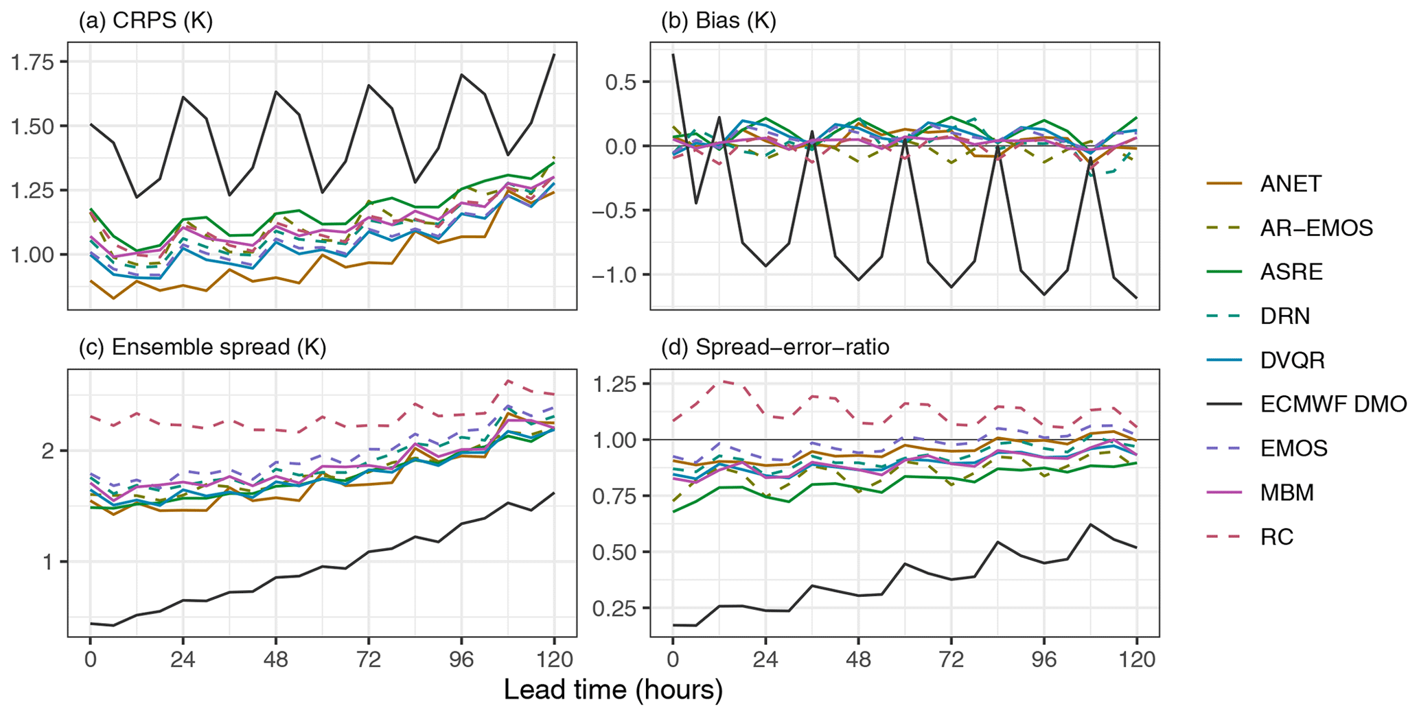
Forecast calibration is assessed with the spread–error ratio (Fig. 3d) and the rank histogram (Fig. 4). ECMWF DMO is heavily overconfident resulting in a spread–error ratio smaller than 1 and a U-shaped rank histogram. Postprocessed forecasts are much better calibrated with indication of some remaining forecast overconfidence for all methods but RC (Fig. 3d). The rank histogram in Fig. 4 allows for a different perspective on forecast calibration with indication of forecast overdispersion (inverse U-shape) for many of the postprocessed forecasts.
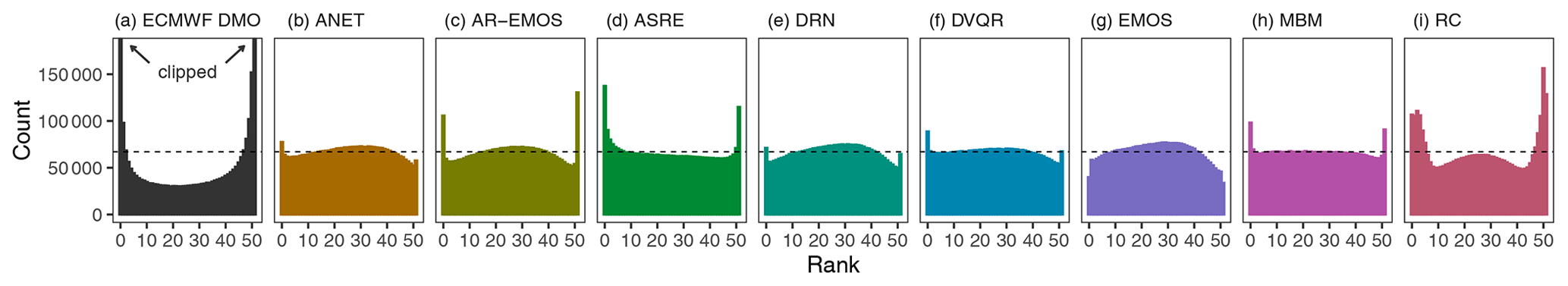
Figure 4Rank histogram of forecasts submitted to the benchmark experiment, aggregated across all stations, forecasts and lead times. Note that the visualization for ECMWF DMO is clipped for better comparison with the rank histograms of the postprocessed forecasts.
Postprocessed forecasts have been produced for a number of stations in central western Europe. With very few exceptions, postprocessing improves forecast quality everywhere as illustrated by the positive values of continuous ranked probability skill score (CRPSS) in Fig. 5. These findings are corroborated by the significance testing presented in Appendix A. Most of the postprocessing methods perform similarly with more pronounced improvements in complex topography and less pronounced improvements in the northern and predominantly flat part of the domain. As a notable exception, ANET forecasts perform better in particular for high-altitude stations in Switzerland (see also Fig. 6).
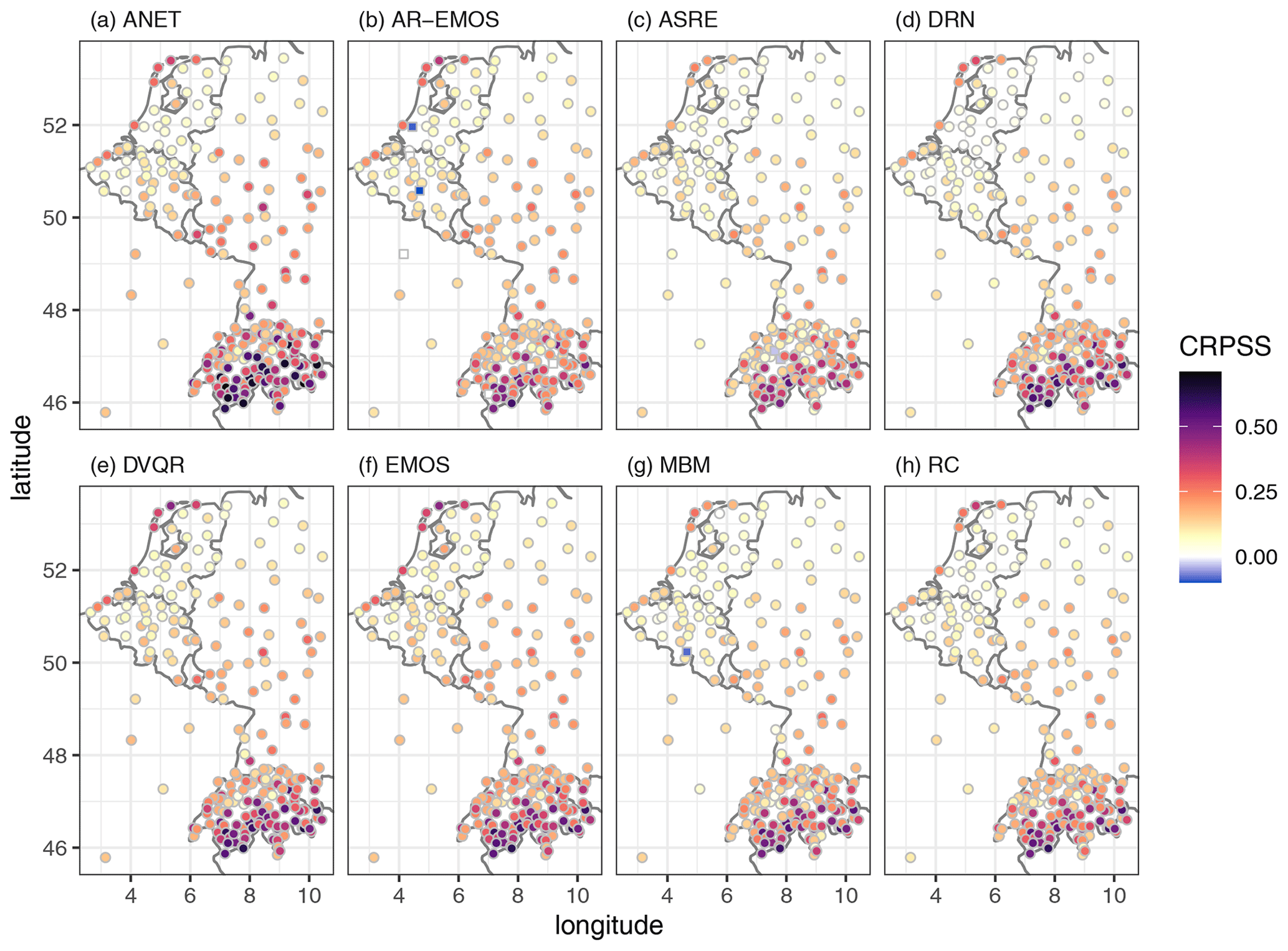
Figure 5Continuous ranked probability skill score (CRPSS) per station, averaged across all forecasts and all lead times. CRPSS is computed using the ECMWF DMO as the reference forecast and positive values indicate that the postprocessed forecasts outperform ECMWF DMO. Stations at which forecast skill is negative are marked by square symbols.
In Fig. 6 we present the relationship with station altitude for a range of scores to further explore the specifics of the postprocessing methods. For example forecasts with the elevation-corrected ECMWF DMO for high-altitude stations are systematically too cold, indicating that the constant lapse rate correction applied to ECMWF DMO is an approximation at best. The AR-EMOS method appears to produce the smallest biases overall, whereas there is some remaining negative bias at altitude in many of the methods and positive biases in RC. The remaining large biases in the AR-EMOS method are from missing predictions that have been filled with ECMWF DMO.
The CRPS at each station in Fig. 6 shows that the reduction in forecast errors and correspondingly increased forecast skill is generally more pronounced at altitude. Compared with the other postprocessing approaches, ANET achieves lower CRPS for high-altitude stations (above 1000 m).
The spread–error ratio as a necessary condition for forecast calibration also reveals considerable differences between postprocessing approaches. The ASRE and RC methods in particular exhibit large variations in spread–error ratio from station to station, whereas the other methods exhibit much more uniform spread–error ratios. Please note that the strong underdispersion of ECMWF DMO as indicated by the spread–error ratio in Figs. 3 and 6 is slightly reduced when systematic biases are removed (not shown). For the postprocessed forecasts, the effect of remaining systematic biases on the spread–error ratio is negligible. More detailed analyses of the results would of course be possible but are beyond the scope of this publication on the benchmark dataset, and they will be the subject of a dedicated work.
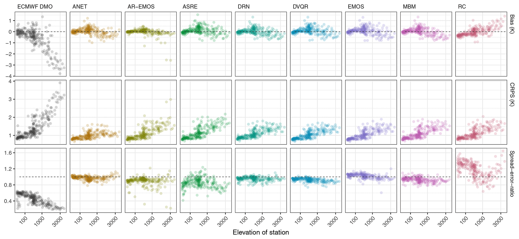
Figure 6Average scores ordered by station elevation; the elevation-corrected ECMWF DMO is shown alongside the results from the postprocessing methods submitted to the benchmark experiment, aggregated across all forecasts and all lead times.
The most straightforward way to access the dataset is through the climetlab (https://github.com/ecmwf/climetlab, last access: 22 December 2022) EUMETNET postprocessing benchmark plugin at https://github.com/EUPP-benchmark/climetlab-eumetnet-postprocessing-benchmark (last access: 31 December 2022). This plugin provides easy access to the dataset stored on the ECMWF European Weather Cloud. An example showing how to use the plugin is documented in the Supplement, along with other unofficial ways to access the data.
In addition, the dataset has been uploaded in Zarr format on Zenodo for long-term storage. See Demaeyer (2022b) (https://doi.org/10.5281/zenodo.7429236) for the gridded data and Bhend et al. (2023) (https://doi.org/10.5281/zenodo.7708362) for the station data.
However, the Switzerland station data which are part of the dataset are not presently freely available. These station data may be obtained from IDAWEB (https://gate.meteoswiss.ch/idaweb/, last access: 15 May 2023) at MeteoSwiss, and we are not entitled to provide it online. Registration with IDAWEB can be initiated here: https://gate.meteoswiss.ch/idaweb/prepareRegistration.do (last access: 15 May 2023). For more information, please also read https://gate.meteoswiss.ch/idaweb/more.do?language=en (last access: 15 May 2023).
The documentation of the dataset is available at https://eupp-benchmark.github.io/EUPPBench-doc/files/EUPPBench_datasets.html (EUMETNET, 2023) and is also provided in the Supplement.
The code and scripts used to perform the benchmark are available on GitHub and have been centralized in a single repository: https://github.com/EUPP-benchmark/ESSD-benchmark (last access: 24 April 2023). This repository contains links to the scripts sub-repositories along with a detailed description of each method. In addition, these codes have been also uploaded to Zenodo: verification code (https://doi.org/10.5281/zenodo.7484371; Primo-Ramos et al., 2023), MBM method (https://doi.org/10.5281/zenodo.7476673, Demaeyer, 2023), reliability calibration method (https://doi.org/10.5281/zenodo.7476590; Evans and Hooper, 2023), ASRE method (https://doi.org/10.5281/zenodo.7477735; Ben Bouallègue, 2023), EMOS method (https://doi.org/10.5281/zenodo.7477749; Dabernig, 2023), AR-EMOS method (https://doi.org/10.5281/zenodo.7477633; Möller, 2023), DRN method (https://doi.org/10.5281/zenodo.7477698; Chen et al., 2023b), DVQR method (https://doi.org/10.5281/zenodo.7477640; Jobst, 2023), and ANET method (https://doi.org/10.5281/zenodo.7479333, Mlakar et al., 2023b).
Finally, to allow for further studies and a better reproducibility, the output data (the corrected forecasts) provided by each method have also been uploaded to Zenodo (See https://doi.org/10.5281/zenodo.7798350, Chen et al., 2023a).
A benchmark dataset is proposed in the context of the EUMETNET postprocessing (EUPP) program for comparing statistical postprocessing techniques that are nowadays an integral part of many operational weather-forecasting suites. This dataset includes ensemble forecasts and reforecasts of the ECMWF for the period 2017–2018, as well as the corresponding gridded and station observations, over a region covering a small portion of western Europe. This region covers a variety of topographies including coastal, flat and mountainous areas. To illustrate the usefulness of this dataset, a standardized exercise is established in order to allow for an objective and rigorous intercomparison of postprocessing methods. This exercise included the contribution of many well-established state-of-the-art postprocessing techniques. Despite the limited scope of the presented exercise, this collaborative effort will serve as a reference framework and will be strongly extended. The whole process includes (i) the download of the data or their access on the European Weather Cloud (where the dataset is stored; see Sect. 6), (ii) the application of the different techniques by the contributors and (iii) the verification of the results by the verification team. This proof-of-concept proved to be very successful.
While the authors constructed and performed this benchmark, some lessons were learned along the way:
-
As much as possible, avoid maintaining an archive or a database of scores for the experiments. Instead compute verification results for the experiments on the fly and only store the summary results. This has the advantage that you can easily add (or remove) scores, summaries of scores, without going through the complex process necessary to update an archive (with new submissions and additional scores).
-
Either be very strict about the format of submitted predictions, or use software that is aware of the NetCDF data model and that can handle slight inconsistencies (e.g., reordering of dimensions or dimension values)
-
Quality control is imperative. While the verification results generally quickly indicate whether there are any major issues with the submitted predictions, issues may already arise earlier than that (making verification impossible). Catching these errors and establishing a feedback loop with the submitters is important. One way to solve this with NetCDF format is to check the NetCDF header of the submission for format compliance.
These points are important for the next EUPP projects, which will aim to harness the full potential of this dataset, by postprocessing other, less predictable variables (e.g., rainfall, radiation), on station and gridded data, and by allowing many predictors instead of only the target variable itself, which can be expected to yield substantial improvements in predictive performance, in particular for the more advanced machine learning approaches (Rasp and Lerch, 2018). By considering broader aspects of forecasting (e.g., spatial and temporal aspects) as well as more specific scores, the verification task for these forthcoming studies will allow us to use more advanced and cutting-edge concepts in the field. The lessons learned from these experiments will also be valuable to other groups engaging with the design and operation of such benchmarking experiments. Ultimately, one of the long-term goals of the current benchmark is to provide an automated procedure to upload and compare new approaches to the existing pool of methods available. It is an ambitious goal, with many challenges ahead, but the benefits it will bring make it worth pursuing.
To assess the significance of the CRPS differences observed between each pair of postprocessing methods in the benchmark results, we compute the percentage of station and lead time combinations for which a standard t test of the null hypothesis of equal predictive performance indicates a significant difference at a level of 5 %. The p values of these tests have been adjusted for multiple testing by controlling the false discovery rate using the Benjamini–Hochberg procedure (Benjamini and Hochberg, 1995). The results are shown in Fig. A1, where each cell in the table shows for what percentage of the station and lead time combinations the method denoted in the row performs significantly better than the method denoted in the column. From this, additional conclusions can be drawn. For instance, all the methods produce a large fraction of significantly better forecasts (i.e., with a lower CRPS) than the ECMWF DMO, while ANET, EMOS, DVQR and AR-EMOS outperform the other methods.
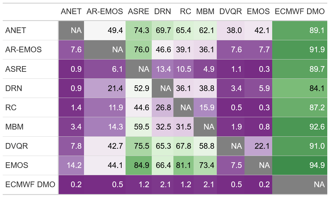
Figure A1Percentage of station and lead time combinations for which the forecast denoted in the row performs significantly (at 5 % level) better in terms of the CRPS than the forecast denoted in the column. The p values have been adjusted for multiple testing using the Benjamini–Hochberg correction.
The supplement related to this article is available online at: https://doi.org/10.5194/essd-15-2635-2023-supplement.
JD led the overall coordination of the benchmark, as well as the collection and dissemination of the dataset. He further contributed to the verification setup, implemented the MBM method (Sect. 4.3) and coordinated the writing of the paper. JC and NH implemented the DRN method (Sect. 4.7). SL coordinated the writing of Sect. 4 and contributed to the implementation of DRN (Sect. 4.7). AM implemented the AR-EMOS method (Sect. 4.5). CP coordinated the verification work and the writing of Sect. 3.2. GE and BH utilized the IMPROVER codebase to implement the reliability calibration method, along with bias correction approaches (Sect. 4.2). MD participated in the collection of the data and provided EMOS corrected forecasts (Sect. 4.4). BVS contributed to the verification results (Sect. 3.2). DJ implemented the DVQR method (Sect. 4.6). AA contributed to the verification work. JB participated in the collection of the data, contributed to the verification work by producing Figs. 3–6 and drafted the Results (Sect. 5). ZBB implemented the ASRE postprocessing method (Sect. 4.1). SV leads the PP module of EUMETNET within which the benchmark has been conceptualized. PM developed and implemented the ANET method (Sect. 4.8). JM and JFP contributed to the development and implementation of the ANET method (Sect. 4.8). OM and MT participated in the collection of the data. All the authors participated to the writing and the review of the paper.
The contact author has declared that none of the authors has any competing interests.
Publisher’s note: Copernicus Publications remains neutral with regard to jurisdictional claims in published maps and institutional affiliations.
This article is part of the special issue “Benchmark datasets and machine learning algorithms for Earth system science data (ESSD/GMD inter-journal SI)”. It is not associated with a conference.
Jonathan Demaeyer thanks Florian Pinault and Baudoin Raoult from ECMWF for their help on the setup of the climetlab plugin, and Francesco Ragone, Lesley De Cruz and David Docquier from Royal Meteorological Institute of Belgium (RMIB) for their support to gather the gridded data. Jonathan Demaeyer also thanks Veerle De Bock and Joffrey Schmitz for their help with the RMIB data. The authors thank Tom Hamill for his guidance on the selection of variables during the dataset design phase. They also thank Thomas Muschinski and Reto Stauffer for raising an important issue about the station data which has since been corrected.
This benchmark activity organized within the postprocessing module of the 2019–2023 EUMETNET program phase is largely supported financially by its members, constituted by a large number of European national meteorological and hydrological services. The EUMETNET postprocessing module also thanks the ECMWF for its support on the European Weather Cloud. Jieyu Chen, Nina Horat and Sebastian Lerch gratefully acknowledge support by the Vector Stiftung through the Young Investigator Group “Artificial Intelligence for Probabilistic Weather Forecasting”. Annette Möller acknowledges support by the Deutsche Forschungsgemeinschaft (DFG, grant no. MO 3394/1-1); by the Hungarian National Research, Development and Innovation Office (under grant no. NN125679); and by the Helmholtz Association's pilot project “Uncertainty Quantification”. Finally, the authors would like to thank the three anonymous reviewers who helped us to increase the value of this paper.
This research has been supported by the 2019–2023 EUMETNET program, the Vector Stiftung (Artificial Intelligence for Probabilistic Weather Forecasting), the Deutsche Forschungsgemeinschaft (grant no. MO 3394/1-1), the Helmholtz Association (grant no. Uncertainty Quantification), and the Hungarian National Research, Development and Innovation Office under grant number NN125679.
This paper was edited by Giuseppe M. R. Manzella and reviewed by three anonymous referees.
Ashkboos, S., Huang, L., Dryden, N., Ben-Nun, T., Dueben, P., Gianinazzi, L., Kummer, L., and Hoefler, T.: Ens-10: A dataset for post-processing ensemble weather forecast, arXiv [preprint], https://doi.org/10.48550/arXiv.2206.14786, 29 June 2022. a, b
Ben Bouallègue, Z.: Accounting for representativeness in the verification of ensemble forecasts, ECMWF Technical Memoranda, 865, https://doi.org/10.21957/5z6esc7wr, 2020. a
Ben Bouallègue, Z.: EUPP-benchmark/ESSD-ASRE: version 1.0 release, Zenodo [code], https://doi.org/10.5281/zenodo.7477735, 2023. a
Benjamini, Y. and Hochberg, Y.: Controlling the False Discovery Rate: A Practical and Powerful Approach to Multiple Testing, J. Roy. Stat. Soc. B Met., 57, 289–300, https://doi.org/10.1111/j.2517-6161.1995.tb02031.x, 1995. a
Bhend, J., Dabernig, M., Demaeyer, J., Mestre, O., and Taillardat, M.: EUPPBench postprocessing benchmark dataset – station data, Zenodo [data set], https://doi.org/10.5281/zenodo.7708362, 2023. a, b
Bremnes, J. B.: Ensemble postprocessing using quantile function regression based on neural networks and Bernstein polynomials, Mon. Weather Rev., 148, 403–414, 2020. a
Chapman, W. E., Monache, L. D., Alessandrini, S., Subramanian, A. C., Ralph, F. M., Xie, S.-P., Lerch, S., and Hayatbini, N.: Probabilistic Predictions from Deterministic Atmospheric River Forecasts with Deep Learning, Mon. Weather Rev., 150, 215–234, https://doi.org/10.1175/MWR-D-21-0106.1, 2022. a
Chen, J., Janke, T., Steinke, F., and Lerch, S.: Generative machine learning methods for multivariate ensemble post-processing, arXiv [preprint], https://doi.org/10.48550/arXiv.2211.01345, 26 September 2022. a
Chen, J., Dabernig, M., Demaeyer, J., Evans, G., Faganeli Pucer, J., Hooper, B., Horat, N., Jobst, D., Lerch, S., Mlakar, P., Möller, A., Merše, J., and Bouallègue, Z. B.: ESSD benchmark output data, Zenodo [data set], https://doi.org/10.5281/zenodo.7798350, 2023a. a
Chen, J., Horat, N., and Lerch, S.: EUPP-benchmark/ESSD-DRN: version 1.0 release, Zenodo [code], https://doi.org/10.5281/zenodo.7477698, 2023b. a
Copernicus Land Monitoring Service, E. U.: CORINE Land Cover, European Environment Agency, CLC, https://land.copernicus.eu/pan-european/corine-land-cover (last access: 30 July 2023), 2018. a, b
Copernicus Land Monitoring Service, E. U.: EU-DEM, European Environment Agency, CLC https://land.copernicus.eu/imagery-in-situ/eu-dem, last access: 1 August 2022. a
Dabernig, M.: EUPP-benchmark/ESSD-EMOS: version 1.0 release, Zenodo [code], https://doi.org/10.5281/zenodo.7477749, 2023. a
Dabernig, M., Mayr, G. J., Messner, J. W., and Zeileis, A.: Spatial Ensemble Post-Processing with Standardized Anomalies, Q. J. Roy. Meteor. Soc., 143, 909–916, https://doi.org/10.1002/qj.2975, 2017. a
Demaeyer, J.: Climdyn/pythie: Version 0.1.0 alpha release, Zenodo [code], https://doi.org/10.5281/zenodo.7233538, 2022a. a
Demaeyer, J.: EUPPBench postprocessing benchmark dataset – gridded data – Part I, Zenodo [data set], https://doi.org/10.5281/zenodo.7429236, 2022b. a, b
Demaeyer, J.: EUPP-benchmark/ESSD-mbm: version 1.0 release, Zenodo [code], https://doi.org/10.5281/zenodo.7476673, 2023. a
Demaeyer, J. and Vannitsem, S.: Correcting for model changes in statistical postprocessing – an approach based on response theory, Nonlin. Processes Geophys., 27, 307–327, https://doi.org/10.5194/npg-27-307-2020, 2020. a
Dueben, P. D., Schultz, M. G., Chantry, M., Gagne, D. J., Hall, D. M., and McGovern, A.: Challenges and Benchmark Datasets for Machine Learning in the Atmospheric Sciences: Definition, Status, and Outlook, Artificial Intelligence for the Earth Systems, 1, e210002, https://doi.org/10.1175/AIES-D-21-0002.1, 2022. a
Eaton, B., Gregory, J., Drach, B., Taylor, K., Hankin, S., Caron, J., Signell, R., Bentley, P., Rappa, G., Höck, H., Pamment, A., Juckes, M., Raspaud, M., Horne, R., Whiteaker, T., Blodgett, D., Zender, C., and Lee, D.: NetCDF Climate and Forecast (CF) metadata conventions, http://cfconventions.org/Data/cf-conventions/cf-conventions-1.8/cf-conventions.pdf (last access: 2 June 2023), 2003. a
EUMETNET: EUPPBench datasets documentation, EUMETNET [data set], https://eupp-benchmark.github.io/EUPPBench-doc/files/EUPPBench_datasets.html, last access: 2023. a
Evans, G. and Hooper, B.: EUPP-benchmark/ESSD-reliability-calibration: version 1.0 release, Zenodo [code], https://doi.org/10.5281/zenodo.7476590, 2023. a
Flowerdew, J.: Calibrating ensemble reliability whilst preserving spatial structure, Tellus A, 66, 22662, https://doi.org/10.3402/tellusa.v66.22662, 2014. a, b
Garg, S., Rasp, S., and Thuerey, N.: WeatherBench Probability: A benchmark dataset for probabilistic medium-range weather forecasting along with deep learning baseline models, arXiv [preprint], https://doi.org/10.48550/arXiv.2205.00865, 2 May 2022. a
Glahn, H. R. and Lowry, D. A.: The use of model output statistics (MOS) in objective weather forecasting, J. Appl. Meteorol. Clim., 11, 1203–1211, 1972. a
Gneiting, T., Raftery, A. E., Westveld, A. H., and Goldman, T.: Calibrated probabilistic forecasting using ensemble model output statistics and minimum CRPS estimation, Mon. Weather Rev., 133, 1098–1118, 2005. a, b
Gregory, J.: The CF metadata standard, CLIVAR Exchanges, 8, 4, http://cfconventions.org/Data/cf-documents/overview/article.pdf (last access: June 2022), 2003. a
Groß, J. and Möller, A.: ensAR: Autoregressive postprocessing methods for ensemble forecasts, R package version 0.2.0, https://github.com/JuGross/ensAR (last access: 2 June 2023), 2019. a
Hafizi, H. and Sorman, A. A.: Assessment of 13 Gridded Precipitation Datasets for Hydrological Modeling in a Mountainous Basin, Atmosphere, 13, 143, https://doi.org/10.3390/atmos13010143, 2022. a
Hagedorn, R., Hamill, T. M., and Whitaker, J. S.: Probabilistic Forecast Calibration Using ECMWF and GFS Ensemble Reforecasts. Part I: Two-Meter Temperatures, Mon. Weather Rev., 136, 2608–2619, https://doi.org/10.1175/2007MWR2410.1, 2008. a
Hamill, T. M., Hagedorn, R., and Whitaker, J. S.: Probabilistic Forecast Calibration Using ECMWF and GFS Ensemble Reforecasts. Part II: Precipitation, Mon. Weather Rev., 136, 2620–2632, https://doi.org/10.1175/2007MWR2411.1, 2008. a
Han, J., Miao, C., Gou, J., Zheng, H., Zhang, Q., and Guo, X.: A new daily gridded precipitation dataset based on gauge observations across mainland China, Earth Syst. Sci. Data Discuss. [preprint], https://doi.org/10.5194/essd-2022-373, in review, 2022. a
Haupt, S. E., Chapman, W., Adams, S. V., Kirkwood, C., Hosking, J. S., Robinson, N. H., Lerch, S., and Subramanian, A. C.: Towards implementing artificial intelligence post-processing in weather and climate: proposed actions from the Oxford 2019 workshop, Philos. T. Roy. Soc. A, 379, 20200091, https://doi.org/10.1098/rsta.2020.0091, 2021. a, b
Hersbach, H.: Decomposition of the continuous ranked probability score for ensemble prediction systems, Weather Forecast., 15, 559–570, 2000. a
Hersbach, H., Bell, B., Berrisford, P., Hirahara, S., Horányi, A., Muñoz-Sabater, J., Nicolas, J., Peubey, C., Radu, R., Schepers, D., Simmons, A., Soci, C., Abdalla, S., Abellan, X., Balsamo, G., Bechtold, P., Biavati, G., Bidlot, J., Bonavita, M., De Chiara, G., Dahlgren, P., Dee, D., Diamantakis, M., Dragani, R., Flemming, J., Forbes, R., Fuentes, M., Geer, A., Haimberger, L., Healy, S., Hogan, R. J., Hólm, E., Janisková, M., Keeley, S., Laloyaux, P., Lopez, P., Lupu, C., Radnoti, G., de Rosnay, P., Rozum, I., Vamborg, F., Villaume, S., and Thépaut, J.-N.: The ERA5 global reanalysis, Q. J. Roy. Meteor. Soc., 146, 1999–2049, https://doi.org/10.1002/qj.3803, 2020. a
Horton, P.: Analogue methods and ERA5: Benefits and pitfalls, Int. J. Climatol., 42, 4078–4096, https://doi.org/10.1002/joc.7484, 2022. a
Hoyer, S. and Joseph, H.: xarray: N-D labeled Arrays and Datasets in Python, Journal of Open Research Software, 5, 10, https://doi.org/10.5334/jors.148, 2017. a
Jobst, D.: EUPP-benchmark/ESSD-DVQR: version 1.0 release, Zenodo [code], https://doi.org/10.5281/zenodo.7477640, 2023. a
Kim, T., Ho, N., Kim, D., and Yun, S.-Y.: Benchmark Dataset for Precipitation Forecasting by Post-Processing the Numerical Weather Prediction, arXiv [preprint], https://doi.org/10.48550/arXiv.2206.15241, 30 June 2022. a
Klein, W. H. and Lewis, F.: Computer Forecasts of Maximum and Minimum Temperatures, J. Appl. Meteorol. Clim., 9, 350–359, https://doi.org/10.1175/1520-0450(1970)009<0350:CFOMAM>2.0.CO;2, 1970. a, b
Klein, W. H., Lewis, B. M., and Enger, I.: Objective prediction of five-day mean temperatures during winter, J. Atmos. Sci., 16, 672–682, 1959. a, b
Kraus, D. and Czado, C.: D-vine copula based quantile regression, Comput. Stat. Data An., 110, 1–18, https://doi.org/10.1016/j.csda.2016.12.009, 2017. a
Lakatos, M., Lerch, S., Hemri, S., and Baran, S.: Comparison of multivariate post-processing methods using global ECMWF ensemble forecasts, Q. J. Roy. Meteor. Soc., 149, 856–877, https://doi.org/10.1002/qj.4436, 2023. a
Lalaurette, F.: Early detection of abnormal weather conditions using a probabilistic extreme forecast index, Q. J. Roy. Meteor. Soc., 129, 3037–3057, 2003. a
Lang, M. N., Lerch, S., Mayr, G. J., Simon, T., Stauffer, R., and Zeileis, A.: Remember the past: a comparison of time-adaptive training schemes for non-homogeneous regression, Nonlin. Processes Geophys., 27, 23–34, https://doi.org/10.5194/npg-27-23-2020, 2020. a
Lenkoski, A., Kolstad, E. W., and Thorarinsdottir, T. L.: A Benchmarking Dataset for Seasonal Weather Forecasts, NR-notat, https://nr.brage.unit.no/nr-xmlui/bitstream/handle/11250/2976154/manual.pdf (last access: 22 December 2022), 2022. a
Lerch, S., Baran, S., Möller, A., Groß, J., Schefzik, R., Hemri, S., and Graeter, M.: Simulation-based comparison of multivariate ensemble post-processing methods, Nonlin. Processes Geophys., 27, 349–371, https://doi.org/10.5194/npg-27-349-2020, 2020. a
Maciel, P., Quintino, T., Modigliani, U., Dando, P., Raoult, B., Deconinck, W., Rathgeber, F., and Simarro, C.: The new ECMWF interpolation package MIR, 36–39, https://doi.org/10.21957/h20rz8, 2017. a
Messner, J. W., Mayr, G. J., and Zeileis, A.: Heteroscedastic Censored and Truncated Regression with crch, The R Journal, 8, 173–181, https://journal.r-project.org/archive/2016-1/messner-mayr-zeileis.pdf (last access: 2 June 2023), 2016. a
Miles, A., Kirkham, J., Durant, M., Bourbeau, J., Onalan, T., Hamman, J., Patel, Z., shikharsg, Rocklin, M., raphael dussin, Schut, V., de Andrade, E. S., Abernathey, R., Noyes, C., sbalmer, pyup.io bot, Tran, T., Saalfeld, S., Swaney, J., Moore, J., Jevnik, J., Kelleher, J., Funke, J., Sakkis, G., Barnes, C., and Banihirwe, A.: zarr-developers/zarr-python: v2.4.0, Zenodo [code], https://doi.org/10.5281/zenodo.3773450, 2020. a
Mlakar, P., Merše, J., and Pucer, J. F.: Ensemble weather forecast post-processing with a flexible probabilistic neural network approach, arXiv [preprint], https://doi.org/10.48550/arXiv.2303.17610, 29 March 2023a. a
Mlakar, P., Pucer, J. F., and Merše, J.: EUPP-benchmark/ESSD-ANET: version 1.0 release, Zenodo [code], https://doi.org/10.5281/zenodo.7479333, 2023b. a
Möller, A.: EUPP-benchmark/ESSD-AR-EMOS: version 1.0 release, Zenodo [code], https://doi.org/10.5281/zenodo.7477633, 2023. a
Möller, A. and Groß, J.: Probabilistic temperature forecasting based on an ensemble autoregressive modification, Q. J. Roy. Meteor. Soc., 142, 1385–1394, https://doi.org/10.1002/qj.2741, 2016. a
Möller, A. and Groß, J.: Probabilistic Temperature Forecasting with a Heteroscedastic Autoregressive Ensemble Postprocessing model, Q. J. Roy. Meteor. Soc., 146, 211–224, https://doi.org/10.1002/qj.3667, 2020. a
Möller, A., Spazzini, L., Kraus, D., Nagler, T., and Czado, C.: Vine copula based post-processing of ensemble forecasts for temperature, arXiv [preprint], https://doi.org/10.48550/arXiv.1811.02255, 6 November 2018. a
Murphy, A. H.: What Is a Good Forecast? An Essay on the Nature of Goodness in Weather Forecasting, Weather Forecast., 8, 281–293, https://doi.org/10.1175/1520-0434(1993)008<0281:WIAGFA>2.0.CO;2, 1993. a
Nagler, T.: vinereg: D-Vine Quantile Regression, r package version 0.7.2, CRAN [code], https://CRAN.R-project.org/package=vinereg (last access: 17 November 2020), 2020. a
Perrone, E., Schicker, I., and Lang, M. N.: A case study of empirical copula methods for the statistical correction of forecasts of the ALADIN-LAEF system, Meteorol. Z., 29, 277–288, https://doi.org/10.1127/metz/2020/1034, 2020. a
Primo-Ramos, C., Bhend, J., Atencia, A., Van schaeybroeck, B., and Demaeyer, J.: EUPP-benchmark/ESSD-Verification: version 1.0 release, Zenodo [code], https://doi.org/10.5281/zenodo.7484371, 2023. a
Rabault, J., Müller, M., Voermans, J., Brazhnikov, D., Turnbull, I., Marchenko, A., Biuw, M., Nose, T., Waseda, T., Johansson, M., Breivik, Ø., Sutherland, G., Hole, L. R., Johnson, M., Jensen, A., Gundersen, O., Kristoffersen, Y., Babanin, A., Tedesco, P., Christensen, K. H., Kristiansen, M., Hope, G., Kodaira, T., de Aguiar, V., Taelman, C., Quigley, C. P., Filchuk, K., and Mahoney, A. R.: A dataset of direct observations of sea ice drift and waves in ice, arXiv [preprint], https://doi.org/10.48550/arXiv.2211.03565, 25 October 2022. a
Raftery, A. E., Gneiting, T., Balabdaoui, F., and Polakowski, M.: Using Bayesian model averaging to calibrate forecast ensembles, Mon. Weather Rev., 133, 1155–1174, 2005. a
Rasp, S. and Lerch, S.: Neural networks for postprocessing ensemble weather forecasts, Mon. Weather Rev., 146, 3885–3900, 2018. a, b, c, d, e, f
Rasp, S., Dueben, P. D., Scher, S., Weyn, J. A., Mouatadid, S., and Thuerey, N.: WeatherBench: A Benchmark Data Set for Data-Driven Weather Forecasting, J. Adv. Model. Earth Sy., 12, e2020MS002203, https://doi.org/10.1029/2020MS002203, 2020. a
Roberts, N., Ayliffe, B., Evans, G., Moseley, S., Rust, F., Sandford, C., Trzeciak, T., Abernethy, P., Beard, L., Crosswaite, N., Fitzpatrick, B., Flowerdew, J., Gale, T., Holly, L., Hopkinson, A., Hurst, K., Jackson, S., Jones, C., Mylne, K., Sampson, C., Sharpe, M., Wright, B., Backhouse, S., Baker, M., Brierley, D., Booton, A., Bysouth, C., Coulson, R., Coultas, S., Crocker, R., Harbord, R., Howard, K., Hughes, T., Mittermaier, M., Petch, J., Pillinger, T., Smart, V., Smith, E., and Worsfold, M.: IMPROVER: the new probabilistic post processing system at the UK Met Office, B. Am. Meteorol. Soc., 104, E680–E697, https://doi.org/10.1175/BAMS-D-21-0273.1, 2023. a
Schulz, B. and Lerch, S.: Machine learning methods for postprocessing ensemble forecasts of wind gusts: A systematic comparison, Mon. Weather Rev., 150, 235–257, 2022. a, b
Taillardat, M., Mestre, O., Zamo, M., and Naveau, P.: Calibrated ensemble forecasts using quantile regression forests and ensemble model output statistics, Mon. Weather Rev., 144, 2375–2393, 2016. a
Vannitsem, S., Wilks, D. S., and Messner, J. W.: Statistical Postprocessing of Ensemble Forecasts, 1st edn., edited by: Vannitsem, S., Wilks, D. S., and Messner, J. W., Elsevier, ISBN 978-0-12-812372-0, 2018. a
Vannitsem, S., Bremnes, J. B., Demaeyer, J., Evans, G. R., Flowerdew, J., Hemri, S., Lerch, S., Roberts, N., Theis, S., Atencia, A., Bouallègue, Z. B., Bhend, J., Dabernig, M., Cruz, L. D., Hieta, L., Mestre, O., Moret, L., Plenković, I. O., Schmeits, M., Taillardat, M., den Bergh, J. V., Schaeybroeck, B. V., Whan, K., and Ylhaisi, J.: Statistical Postprocessing for Weather Forecasts: Review, Challenges, and Avenues in a Big Data World, B. Am. Meteorol. Soc., 102, E681–E699, https://doi.org/10.1175/BAMS-D-19-0308.1, 2021. a, b
Van Schaeybroeck, B. and Vannitsem, S.: Ensemble post-processing using member-by-member approaches: theoretical aspects, Q. J. Roy. Meteor. Soc., 141, 807–818, https://doi.org/10.1002/qj.2397, 2015. a
Wang, W., Yang, D., Hong, T., and Kleissl, J.: An archived dataset from the ECMWF Ensemble Prediction System for probabilistic solar power forecasting, Sol. Energy, 248, 64–75, https://doi.org/10.1016/j.solener.2022.10.062, 2022. a
Watson-Parris, D., Rao, Y., Olivié, D., Seland, Ø., Nowack, P., Camps-Valls, G., Stier, P., Bouabid, S., Dewey, M., Fons, E., Gonzalez, J., Harder, P., Jeggle, K., Lenhardt, J., Manshausen, P., Novitasari, M., Ricard, L., and Roesch, C.: ClimateBench v1.0: A Benchmark for Data-Driven Climate Projections, J. Adv. Model. Earth Sy., 14, e2021MS002954, https://doi.org/10.1029/2021MS002954, 2022. a
Wilks, D. S.: Multivariate ensemble Model Output Statistics using empirical copulas, Q. J. Roy. Meteor. Soc., 141, 945–952, https://doi.org/10.1002/qj.2414, 2015. a
Zandler, H., Haag, I., and Samimi, C.: Evaluation needs and temporal performance differences of gridded precipitation products in peripheral mountain regions, Scientific Reports, 9, 15118, https://doi.org/10.1038/s41598-019-51666-z, 2019. a
Zantedeschi, V., Falasca, F., Douglas, A., Strange, R., Kusner, M. J., and Watson-Parris, D.: Cumulo: A dataset for learning cloud classes, arXiv [preprint], https://doi.org/10.48550/arXiv.1911.04227, 5 November 2019. a
Zsótér, E.: Recent developments in extreme weather forecasting, ECMWF Newsletter, 107, 8–17, 2006. a
Commonly abbreviated as “EFI”.
The ensemble forecasts grid O640 has a horizontal resolution of 18 km, while the deterministic forecasts grid O1280 has a 9 km horizontal resolution.
See a detailed list of the methods GitHub repositories at https://github.com/EUPP-benchmark/ESSD-benchmark (last access: 25 April 2023).
- Abstract
- Introduction
- EUPPBench v1.0 dataset
- Postprocessing benchmark
- Postprocessing methods
- Results
- Code and data availability
- Conclusions and prospects
- Appendix A: Significance assessment
- Author contributions
- Competing interests
- Disclaimer
- Special issue statement
- Acknowledgements
- Financial support
- Review statement
- References
- Supplement