A gridded dataset of a leaf-age-dependent leaf area index seasonality product over tropical and subtropical evergreen broadleaved forests

The quantification of large-scale leaf-age-dependent leaf area index has been lacking in tropical and subtropical evergreen broadleaved forests (TEFs), despite the recognized importance of leaf age in influencing leaf photosynthetic capacity in this biome. Here, we simplified the canopy leaves of TEFs into three age cohorts (i.e., young, mature, and old, with different photosynthesis capacities; i.e., V_c,max) and proposed a novel neighbor-based approach to develop the first gridded dataset of a monthly leaf-age-dependent leaf area index (LAI) product (referred to as Lad-LAI) at 0.25^∘ spatial resolution over the continental scale during 2001–2018 from satellite observations of sun-induced chlorophyll fluorescence (SIF) that was reconstructed from MODIS and TROPOMI (the TROPOspheric Monitoring Instrument). The new Lad-LAI products show good performance in capturing the seasonality of three LAI cohorts, i.e., young (LAI_young; the Pearson correlation coefficient of R=0.36), mature (LAI_mature; R=0.77), and old (LAI_old; R=0.59) leaves at eight camera-based observation sites (four in South America, three in subtropical Asia, and one in the Democratic Republic of the Congo (DRC)) and can also represent their interannual dynamics, validated only at the Barro Colorado site, with R being equal to 0.54, 0.64, and 0.49 for LAI_young, LAI_mature, and LAI_old, respectively. Additionally, the abrupt drops in LAI_old are mostly consistent with the seasonal litterfall peaks at 53 in situ measurements across the whole tropical region (R=0.82). The LAI seasonality of young and mature leaves also agrees well with the seasonal dynamics of the enhanced vegetation index (EVI; R=0.61), which is a proxy for photosynthetically effective leaves. Spatially, the gridded Lad-LAI data capture a dry-season green-up of canopy leaves across the wet Amazonian areas, where mean annual precipitation exceeds 2000 mm yr⁻¹, consistent with previous satellite-based analyses. The spatial patterns clustered from the three LAI cohorts also coincide with those clustered from climatic variables over the whole TEF region. Herein, we provide the average seasonality of three LAI cohorts as the main dataset and their time series as a supplementary dataset. These Lad-LAI products are available at https://doi.org/10.6084/m9.figshare.21700955.v4 (Yang et al., 2022).

1 Introduction

Tropical and subtropical evergreen broadleaved forests (TEFs) account for approximately 34 % of global terrestrial primary productivity (GPP; Beer et al., 2010) and 40 %–50 % of the world's gross forest carbon sink (Pan et al., 2011; Saatchi et al., 2011). Despite a perennial canopy, TEFs shed and rejuvenate their leaves continuously throughout the year, leading to significant seasonality in canopy leaf demography (Wu et al., 2016; Chen et al., 2021). This phenological change in leaf demography is the primary cause of GPP seasonality in TEFs (Saleska et al., 2003; Sayer et al., 2011; Leff et al., 2012), and this thus largely regulates their seasonal carbon sinks (Beer et al., 2010; Aragao et al., 2014; Saatchi et al., 2011).

A key plant trait linking canopy phenology with GPP seasonality was shown to be leaf age (Wu et al., 2017; Xu et al., 2017). At the leaf scale, the newly flushed young leaves and maturing leaves show higher maximum carboxylation rates (V_c,max) than the old leaves being replaced (De Weirdt et al., 2012; Chen et al., 2020). Such age-dependent variations in V_c,max are associated with changes in leaf nutritional contents (nitrogen, phosphorus, potassium, etc.) and stomatal conductance over time (Menezes et al., 2021). Xu et al. (2017) and Menezes et al. (2021) monitored in situ leaf age and leaf demography combined with leaf-level V_c,max in Amazonian TEFs and found that V_c,max of newly flushed leaves increases rapidly with leaf longevity, peaks at approximately 2 months old, and then declines gradually as leaf grows older (leaf age >2 months). At canopy scale, it was hypothesized that leaf demography and seasonal differences in leaf age compositions of tree canopies control the GPP seasonality in TEFs (Wu et al., 2016; Albert et al., 2018). A similar mechanism was also observed from the ground-based lidar signals which showed an increasing trend in upper canopy leaf area index (LAI) during the dry season, whereas there was a decrease in lower canopy LAI (more old leaves; Smith et al., 2019). Wu et al. (2016) classified the canopy leaves of Amazonian TEFs into three leaf age cohorts (young at 1–2 months, mature at 3–5 months, and old at ≥6 months). The LAI of young and mature leaves increased during the dry seasons and consequently promoted dry-season canopy photosynthesis. Based on the above age-dependent V_c,max at leaf scale (Xu et al., 2017) and the LAI seasonality of different leaf age cohorts at canopy scale (Wu et al., 2016), Chen et al. (2020, 2021) developed a climate-triggered leaf litterfall and flushing model and successfully represented the seasonality of canopy leaf demography and GPP at four Amazonian TEF sites. Overall, leaf-age-dependent LAI seasonality is one of the vital biotic factors in influencing the GPP seasonality in TEFs (Wu et al., 2016; Chen et al., 2020).

Although the leaf-age-dependent LAI seasonality can be well documented at site level using phenology cameras (Wu et al., 2016), it is still rarely studied and remains unclear at the continental scale. The key causation for this is that the leaf flushing and litterfall of TEFs in different climatic regions experience different seasonal constraints of water and light availability during recurrent dry and wet seasons (Brando et al., 2010; Chen et al., 2020; Davidson et al., 2012; Xiao et al., 2005). Thus, the seasonal patterns of LAI in different leaf age cohorts become very complex at the continental scale (Chen et al., 2020; Xu et al., 2015). Satellite-based remote sensing (Saatchi et al., 2011; Guan et al., 2015) and land surface model (LSM) technologies (De Weirdt et al., 2012; Chen et al., 2020, 2021) are two commonly used approaches for detecting the spatial heterogeneity of plant phenology at a large scale. However, for satellite-based studies, most optical signals are saturated in TEFs due to the dense covered canopies and thus fail to capture the seasonality of total LAI in TEFs and are much less able to decompose the LAI into different leaf age cohorts. These limitations prevent satellite-based studies from accurately representing the age-dependent LAI seasonality. Moreover, most Earth system models (ESMs) also show poor performances in simulating the LAI seasonality in different leaf age cohorts (De Weirdt et al., 2012; Chen et al., 2020). This is because the underlying mechanisms linking seasonal water and light availability with leaf flushing and litterfall seasonality are currently highly debated and remain elusive at the regional scale (Leff et al., 2012; Saleska et al., 2003; Sayer et al., 2011). This vague notion imposes a challenge for accurately modeling continental-scale GPP seasonality in most LSMs (Restrepo-Coupe et al., 2017; Chen et al., 2021).

To fill the research gap, this study aimed to produce a global gridded dataset of leaf-age-dependent LAI seasonality product (Lad-LAI) over the whole TEF biomes from 2001 to 2018. For this purpose, we first simplified the canopy GPP as being composed of three parts that were produced from young, mature, and old leaves, respectively. GPP was then expressed as a function of the sum of the product of each LAI cohort (i.e., young, mature, and old leaves, denoted as LAI_young, LAI_mature, and LAI_old, respectively) and corresponding net CO₂ assimilation rate (An, denoted as An_young, An_mature, and An_old for young, mature, and old leaves, respectively; Eq. 1). Then, we proposed a novel neighbor-based approach to derive the values of three LAI cohorts. It was hypothesized that forests in the adjacent four cells in the gridded map exhibited consistent seasonality in both GPP and LAI cohorts (LAI_young, LAI_mature, and LAI_old). Based on this assumption, we applied Eq. (1) to each pixel and combined the four equations of 2×2 neighboring pixels to derive the three LAI cohorts using a linear least squares with the constrained method. The An parameter was calculated using the Farquhar–von Caemmerer–Berry (FvCB) leaf photochemistry model (Farquhar et al., 1980), and GPP was linearly derived from an arguably better proxy in the form of the TROPOMI (the TROPOspheric Monitoring Instrument) solar-induced fluorescence (SIF), based on a simple SIF–GPP relationship established by Chen et al. (2022; see Sect. 3 for details). This gridded dataset of three LAI cohorts provides new insights into tropical and subtropical phenology, with more details of subcanopy level of leaf seasonality in different leaf age cohorts, and will be helpful for developing an accurate tropical phenology model in ESMs.

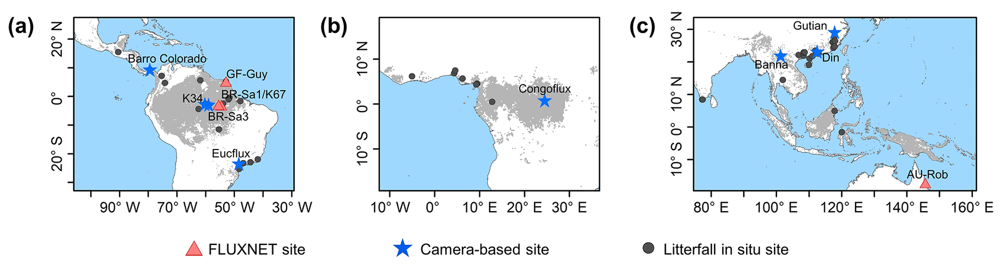
Figure 1 Study areas over tropical and subtropical evergreen broadleaves forests (TEF). Red triangles show the observed GPP seasonality at four eddy covariance (EC) tower sites. Blue pentangles show the observed LAI cohorts at eight camera-based observation sites. Black circles show the observed litterfall seasonality at 53 observation sites.

2 Study area and material

2.1 Tropical and subtropical evergreen broadleaved forest biomes

In this study, we focused on the whole tropical and subtropical evergreen broadleaf forests (TEFs). The pixels labeled TEFs, according to the International Geosphere–Biosphere Program (IGBP) classification, were extracted as the study area, based on the 0.05^∘ spatial resolution MODIS land cover map (Fig. 1; MCD12C1; Sulla-Menashe et al., 2018). The study area contains three regions, namely South America (18^∘ N–30^∘ S, 40–90^∘ W), the world's largest and most biodiverse tropical rain forest, Republic of the Congo and Democratic Republic of the Congo (DRC; 10^∘ N–10^∘ S, 10^∘ W–30^∘ E), the western part of the Africa TEF region, and tropical Asia (30^∘ N–20^∘ S, 70–150^∘ E), covering the Southeast Asian Peninsula, the majority of the Malay Archipelago and northern Australia.

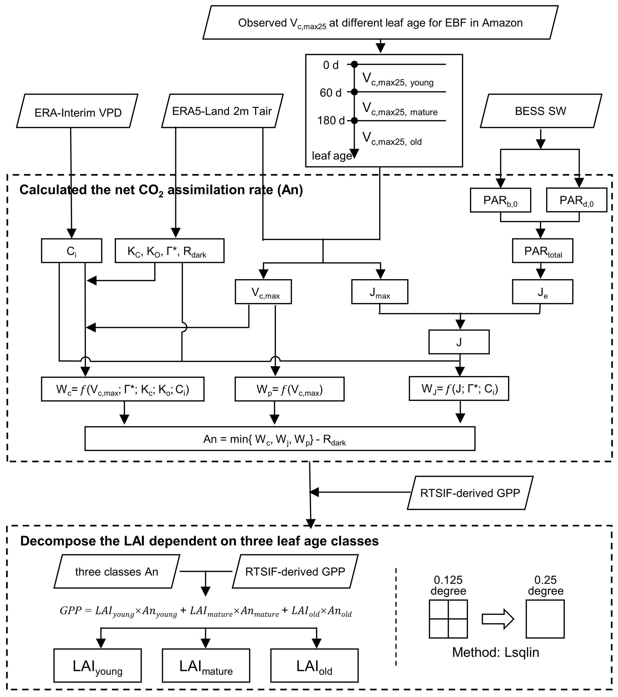
Figure 2 The workflow for mapping Lad-LAI using the Lsqlin method. Lsqlin is the abbreviation of the linear least squares solver with bounds or linear constraints. All the abbreviations are described in Table S4 in the Supplement.

2.2 Input datasets for calculating GPP and An parameters

The TROPOMI SIF data were used to derive the continent-scale GPP (denoted as RTSIF-derived GPP), according to the SIF–GPP relationship established by Chen et al. (2022), which used 15.343 as a transformation coefficient to covert SIF to GPP. The air temperature data from ERA5-Land (Zhao et al., 2020), vapor pressure deficit (VPD) data from ERA-Interim (Yuan et al., 2019), and downward shortwave solar radiation (SW) from the Breathing Earth System Simulator (BESS; Ryu et al., 2018) were used to calculate the Michaelis–Menton constant for carboxylase (K_c), the Michaelis–Menton constant for oxygenase (K_o), the CO₂ compensation point (Γ^*), dark respiration (R_dark), and V_c,max and thus to calculate the An parameter according to the equations in Table S4 (see the Supplement). The calculation processes are illustrated in Fig. 2. All datasets were aggregated at the same spatial (0.125^∘) and temporal resolutions (month; Table S3).

2.3 Datasets for validating leaf-age-dependent LAI seasonality

2.3.1 Ground-based seasonal LAI cohorts and litterfall data

The top-of-canopy imagery observed by ground-based phenology cameras were used to decompose the canopy LAI into LAI_young, LAI_mature, and LAI_old. In total, imagery from eight observation sites across the whole TEF region were used to validate the simulation results (blue pentangles in Fig. 1; Table S1 in the Supplement). Additionally, the seasonal litterfall data from 53 in situ sites (black circles in Fig. 1; Table S6) spanning the TEFs were collected from globally published articles to compare them with the phase of simulated LAI_old seasonality (see Sect. 3 for details). The multiyear monthly litterfall data were averaged to the monthly mean to compare them with the seasonality of the simulated LAI_old. Four eddy covariance flux tower sites (red triangles in Fig. 1; Table S2) provided in situ seasonal GPP data to evaluate the seasonality of RTSIF-derived GPP.

2.3.2 Satellite-based seasonal EVI data

To evaluate the LAI seasonality of photosynthetically effective leaves (i.e., young and mature leaves), this study used the satellite-based MODIS and enhanced vegetation index (EVI; Huete et al., 2002; Lopes et al., 2016; Wu et al., 2018) as the remotely sensed proxied alternatives of effective leaf area changes and new leaf flush (i.e., LAI_young+mature; Wu et al., 2016; Xu et al., 2015). To prove the robustness of the products over a large spatial coverage, the seasonal LAI cohorts of young and mature leaves were evaluated against the EVI product, which was considered to be a proxy for leaf area changes in photosynthetically effective leaves (Xu et al., 2015; Wu et al., 2016; de Moura et al., 2017).

3 Methods

3.1 Decomposing LAI cohorts (young, mature, and old) from SIF-derived GPP

Figure 2 illustrates the overall framework used to generate the leaf-age-dependent LAI seasonality product (Lad-LAI). The majority of the tropical and subtropical TEFs retain leaves year-round, and their total LAI shows marginally small spatial and seasonal changes (Wu et al., 2016; Figs. S3, S4). Therefore, previous modeling studies have assumed a constant value for the total LAI in tropical and subtropical TEFs (Cramer et al., 2001; Arora and Boer, 2005; De Weirdt et al., 2012). Based on this, we collected observed seasonal LAI dynamics in tropical and subtropical TEFs from previously published literature, which showed a constant value of LAI at around 6.0 (Figs. S3, S4; Table S5). Thus, in this study, we simplified the data to assume that the seasonal LAI was approximately equal to 6.0 in tropical and subtropical TEFs. We grouped the canopy leaves of tropical and subtropical TEFs into three leaf age cohorts (i.e., young, mature and old leaves, respectively). Then, the total GPP was defined as the sum of those produced by the young, mature, and old leaves, respectively. According to the FvCB leaf photochemistry model (Farquhar et al., 1980), GPP can be expressed as function of the sum of the products of each LAI cohort (LAI_young, LAI_mature, and LAI_old) and corresponding net CO₂ assimilation rate (An_young, An_mature, and An_old; Eq. 1).

$$\begin{array}{}\text{(1)}& \begin{array}{rl}\mathrm{GPP}& ={\mathrm{LAI}}_{\mathrm{young}}\times {\mathrm{An}}_{\mathrm{young}}+{\mathrm{LAI}}_{\mathrm{mature}}\times {\mathrm{An}}_{\mathrm{mature}}\\ & +{\mathrm{LAI}}_{\mathrm{old}}\times {\mathrm{An}}_{\mathrm{old}},\end{array}\end{array}$$

where LAI_young, LAI_mature, and LAI_old are the leaf area index of young, mature, and old leaves, respectively. An_young, An_mature, and An_old are the net rate of the CO₂ assimilation, dependent on three leaf age classes. GPP is the canopy total gross primary production. The sum of LAI_young, LAI_mature, and LAI_old was set as a constant in this study, equaling to 6.0.

The gridded GPP data over the whole TEFs were derived from SIF (denoted as RTSIF-derived GPP) using a linear SIF–GPP regression model (see Sect. 3.2), which was established based on in situ GPP from 76 eddy covariance (EC) sites (Chen et al., 2022). The An_young, An_mature, and An_old were calculated according to the FvCB biochemical model (Farquhar et al., 1980; Bernacchi et al., 2003; see Sect. 3.3). As there were three unknown variables (i.e., LAI_young, LAI_mature, and LAI_old) to be solved in Eq. (1), we hypothesized that the adjacent four pixels exhibited homogenous TEFs and consistent leaf demography and canopy photosynthesis. Then, we used the GPP and An data from the adjacent four pixels to estimate their LAI_young, LAI_mature, and LAI_old, based on Eq. (1), using linear least squares with the constrained method. The inputs, on gridded datasets (i.e., RTSIF-derived GPP and An derived from T_air, VPD, and SW; Table S3; Fig. 2), were sampled at 0.125^∘ spatial resolution, while the output maps of LAI_young, LAI_mature, and LAI_old were at 0.25^∘ spatial resolution. Therefore, the output maps of LAI_young, LAI_mature, and LAI_old were at a 0.25^∘ spatial resolution. Additionally, to test the robustness of the neighbor-based decomposition approach, we increased the number of adjacent pixels from 4 (2×2) to 16 (4×4) to produce another version of the Lad-LAI product, with a spatial resolution of 0.5^∘. All our analyses were conducted using Python (version 3.7; http://www.python.org, last access: 15 June 2023) and MATLAB (version R2019b) software.

3.2 Calculating the GPP (RTSIF-derived GPP) from TROPOMI SIF

Satellite-retrieved solar-induced chlorophyll fluorescence (SIF) is a widely used proxy for canopy photosynthesis (Yang et al., 2015; Dechant et al., 2020). Here, we used a long-term reconstructed TROPOMI SIF dataset (RTSIF; Chen et al., 2022) to estimate GPP seasonality. Previous analyses showed that RTSIF was strongly linearly correlated to eddy covariance (EC) GPP and used 15.343 as a transformation coefficient to convert RTSIF to GPP (Fig. 8a in Chen et al., 2022). In this study, we followed previously published literature to set a constant value of LAI around 6.0 for the whole tropical and subtropical TEFs (Figs. S3, S4; Table S5). We collected seasonal GPP data observed at four EC sites from the FLUXNET2015 tier 1 dataset (Table S2; Pastorello et al., 2020) and validated the Chen et al. (2022) simple SIF–GPP relationship (Fig. S1 in the Supplement). Results confirmed the robustness of the Chen et al. (2022) simple SIF–GPP relationship for estimating the GPP seasonality in tropical and subtropical TEFs (R>0.49). Despite the potential overestimation (Fig. S1b) or underestimation (Fig. S1h) of the magnitudes, the RTSIF-derived GPP mostly captured the seasonality of the EC GPP at all four sites (d_phase<0.26).

3.3 Calculating the net rate of CO₂ assimilation (An)

We calculated the net CO₂ assimilation (An) using the FvCB biochemical model (Farquhar et al., 1980). In this model, the parameter An was calculated as the minimum of RuBisCO (W_c), RuBP regeneration (W_j), and TPU (W_p) to minus dark respiration (R_dark; Bernacchi et al., 2013). The formulae for calculating An, W_c, W_j, W_p, R_dark, and the corresponding intermediate variables were listed in Table S4.

3.3.1 Calculation of W_c

W_c is expressed as a function of the internal CO₂ concentration (c_i), K_c, K_o, Γ*, and the maximum carboxylation rate (V_c,max; Table S4 part1; Lin et al., 2015; Bernacchi et al., 2013; Ryu et al., 2011; Medlyn et al., 2011; June et al., 2004; Farquhar et al., 1980). The K_c, K_o, Γ*, and V_c,max are temperature-dependent variables. Thus, we used Eq. (2) to calculate their values at T_k by converting from those at 25^∘. Then, we used the Medlyn et al. (2011) stomatal conductance model to estimate internal CO₂ concentration (c_i; Eq. 3), which is expressed as a function of the VPD rather than relative humidity (Lin et al., 2015). The method for calculating the V_c,max of each LAI cohort was introduced in Sect. 3.4. The formulae for calculating corresponding intermediate parameters are presented in Table S4.

$$\begin{array}{}\text{(2)}& \mathrm{Para}={\mathrm{Para}}_{\mathrm{25}}\times \exp \left({\displaystyle \frac{\left(T_{\mathrm{k}}-\mathrm{298.15}\right)\times \mathrm{\Delta }{H}_{\mathrm{para}}}{R\times T_{\mathrm{k}}\times \mathrm{298.15}}}\right),\end{array}$$

where Para denotes a correction factor arising from the temperature dependence of V_c,max, Para₂₅ are values of the temperature-dependent parameters (K_c, K_o, Γ*, and V_c,max) at the temperature 25^∘, T_k denotes temperature in Kelvin, ΔH_para is the activation energy for temperature dependence, and R is the universal gas constant.

$$\begin{array}{}\text{(3)}& c_{\mathrm{i}}=c_{\mathrm{a}}\times \left(\mathrm{1}-{\displaystyle \frac{\mathrm{1}}{\mathrm{1.6}\times \left(\mathrm{1}+\frac{g_{\mathrm{1}}}{\surd \mathrm{VPD}}\right)}}\right),\end{array}$$

where c_a is atmospheric CO₂ concentration (380 ppm – parts per million). VPD is calculated from the air temperature and dew point temperature of the global ERA-Interim reanalysis dataset (Dee et al., 2011), using the method of Yuan et al. (2019). The calculation formula of VPD is described in the Supplement. In this study, we used the value of 3.77 for the stomatal slope (g₁) in the stomatal conductance model, according to Lin et al. (2015).

3.3.2 Calculation of W_p

W_p was calculated as the function of V_c,max, which was given different values for different LAI cohorts based on multiple in situ observations (Sect. 3.4).

3.3.3 Calculation of W_j

W_j was calculated from V_c,max, c_i, and the rate of electrons through the thylakoid membrane (J; Bernacchi et al., 2013). The parameter J was calculated from the maximum electron transport rate (J_max), and the rate of the whole electron transport provided by light (J_e; Bernacchi et al., 2013). J_max was expressed as a temperature-dependent function of the maximum electron transport rate (J_max,25) at 25^∘. Temperature (T_air) and J_e were expressed as a function of total photosynthetically active radiation (PAR) absorbed by the canopy (PAR_total) that was the sum of the active radiation in the beam (PAR_b,0) and the diffused (PAR_d,0) light (Weiss and Norman, 1985), which were calculated from downward shortwave radiation (SW; Ryu et al., 2018). The formula for PAR_total is given in Eq. (4), and the formulae for other intermediate parameters (i.e., PAR_b,0, PAR_d,0, ρ_cb, ρ_cd, $k{{}^{\prime }}_{\mathrm{b}}$, $k{{}^{\prime }}_{\mathrm{d}}$, and CI) are listed in Table S4.

$$\begin{array}{}\text{(4)}& \begin{array}{rl}{\mathrm{PAR}}_{\mathrm{total}}& =\left(\mathrm{1}-{\mathit{\rho }}_{\mathrm{cb}}\right)\times {\mathrm{PAR}}_{\mathrm{b},\mathrm{0}}\\ & \times \left(\mathrm{1}-\exp \left(-k_{\mathrm{b}}{}^{\prime }\times CI\times {\mathrm{LAI}}_{\mathrm{total}}\right)\right)\\ & +\left(\mathrm{1}-{\mathit{\rho }}_{\mathrm{cd}}\right)\times {\mathrm{PAR}}_{\mathrm{d},\mathrm{0}}\\ & \times \left(\mathrm{1}-\exp \left(-k_{\mathrm{d}}{}^{\prime }\times CI\times {\mathrm{LAI}}_{\mathrm{total}}\right)\right),\end{array}\end{array}$$

where PAR_total is total PAR absorbed by the canopy, PAR_b,0 is the active radiation, PAR_d,0 is diffused radiation, and LAI_total is a total LAI. Here, we used a constant value of 6.0, according to De Weirdt et al. (2012).

3.4 Classifying three LAI cohorts with different V_c,max

In this study, we compared in situ samples of V_c,max25 data against different leaf age across tropical and subtropical TEFs from previous publications. Mature leaves (leaf age 70–160 d) show the highest V_c,max25 compared to those of newly flushed leaves (leaf age <60 d) and old leaves (leaf age >200 d), as seen in Menezes et al. (2021). Therefore, in this study, we classified the canopy leaves into three cohorts, namely young (leaf age <2 months), mature (leaf age 3–5 months), and old cohorts (leaf age >6 months), as per Wu et al. (2016). The V_c,max25 values for young, mature, and old cohorts were set to 60, 40, and 20 µmol m⁻² s⁻¹, respectively, according to previous ground-based observations by Chen et al. (2020).

3.5 Decomposing camera-based LAI into three leaf age cohorts

We classified the canopy leaves into young, mature, and old age cohorts based on the green color band from the top-of-canopy imagery observed by a RGB camera. This is because the brightness of different leaf age leaves differs greatly in the values of the green color band. Raster density slicing is a useful classification method for detecting the attributes of various ground objects (Kartikeyan et al., 1998). Therefore, we set three brightness thresholds to divide young (blue), mature (green), and old (yellow) leaves and background (gray) for the same canopy extent in each month (Fig. S2). This analysis was conducted in ENVI 5 Service Pack 3 software.

3.6 Evaluating the LAI_young+mature seasonality and its spatial patterns using satellite-based EVI products

To compare the seasonality of LAI_young+mature with those of EVI, we calculate the mean squared deviation (MSD) and their three components, namely d_bias, which denotes the differences about absolute value, d_var, which denotes the differences in seasonal fluctuations, and d_phase, which denotes the differences in peak phase to evaluate this consistency comprehensively (see Sect. 3.8). Additionally, we compared the spatial patterns of the wet- minus dry-season differences (Δ) between the observed and simulated variables, following the work of Guan et al. (2015). To determine the wet and dry seasons in each grid cell, we defined a month as being a dry one when its monthly average precipitation was smaller than the potential evapotranspiration (PET) computed using the method of Maes et al. (2019); other months were classified as wet ones. The wet- minus dry-season LAI_young+mature (denoted as ΔLAI_young+mature) was calculated for each grid cell as the wet-season average LAI_young+mature value minus the dry-season average value of LAI_young+mature.

3.7 Evaluating the LAI_old seasonality using ground-based litterfall data

Litterfall is closely related to the seasonal dynamics of old leaves (i.e., LAI_old; Chen et al., 2020; Yang et al., 2021). Previous analyses indicated that, in general, a sharp decrease in LAI_old corresponded to a peak in litterfall (Pastorello et al., 2020; Midoko Iponga et al., 2019; Ndakara, 2011; Barlow et al., 2007; Dantas and Phillipson, 1989). Based on this causal relationship between litterfall and LAI_old, we compared the time of seasonal litterfall peak with the time of abrupt drops in LAI_old to indirectly evaluate the simulated LAI_old seasonality. To accurately detect the onset date of old leaves being shed and the day of the litterfall peak, we used a least squares regression analysis method, developed by Piao et al. (2006), to smooth the LAI_old and litterfall seasonal curves. The sixth-degree polynomial function (n=6) was applicable to the regression (Eq. 5).

$$\begin{array}{}\text{(5)}& {\mathrm{LAI}}_{\mathrm{old}}=a_{\mathrm{0}}+a_{\mathrm{1}}x+a_{\mathrm{2}}{x}^{\mathrm{2}}+a_{\mathrm{3}}{x}^{\mathrm{3}}+a_{\mathrm{4}}{x}^{\mathrm{4}}+a_{\mathrm{5}}{x}^{\mathrm{5}}+a_{\mathrm{6}}{x}^{\mathrm{6}},\end{array}$$

where x is the day of a year.

The slope of seasonal LAI (LAI_old, ratio) was calculated in Eq. (6). The date of abrupt drops in LAI_old was defined as the time with the most negative values of LAI_old, ratio.

$$\begin{array}{}\text{(6)}& {\mathrm{LAI}}_{\mathrm{old},\mathrm{ratio}\left(t\right)}=\left({\mathrm{LAI}}_{\mathrm{old}(t+\mathrm{1})}-{\mathrm{LAI}}_{\mathrm{old}\left(t\right)}\right)/\left({\mathrm{LAI}}_{\mathrm{old}\left(t\right)}\right),\end{array}$$

where LAI_old, ratio is the slope of seasonal LAI_old curve. LAI_old(t+1) and LAI_old(t) are the corresponding monthly LAI at times t+1 and t, respectively.

3.8 Evaluation metrics

Two metrics were chosen to evaluate the seasonality of Lad-LAI against the that of other proxies, namely the Kobayashi and Salam (2000) decomposition of the mean square difference between the model and observation and the Pearson (1896) correlation coefficient for gridded fields.

3.8.1 Mean squared deviation (MSD)

The mean squared deviation (MSD) was given by Kobayashi and Salam (2000):

$$\begin{array}{}\text{(7)}& {\displaystyle }\mathrm{MSD}={\displaystyle \frac{\mathrm{1}}{n}}\sum _{i=\mathrm{1}}^n{\left(x_i-y_i\right)}^{\mathrm{2}}\text{(8)}& {\displaystyle }\mathrm{SB}=(\stackrel{\mathrm{‾}}{x}-\stackrel{\mathrm{‾}}{y}{)}^{\mathrm{2}}\text{(9)}& {\displaystyle }{\mathrm{SD}}_{\mathrm{s}}=\sqrt{{\displaystyle \frac{\mathrm{1}}{n}}{\sum }_{i=\mathrm{1}}^n{\left(x_i-\stackrel{\mathrm{‾}}{x}\right)}^{\mathrm{2}}}\text{(10)}& {\displaystyle }{\mathrm{SD}}_{\mathrm{m}}=\sqrt{{\displaystyle \frac{\mathrm{1}}{n}}{\sum }_{i=\mathrm{1}}^n{\left(y_i-\stackrel{\mathrm{‾}}{y}\right)}^{\mathrm{2}}}\text{(11)}& {\displaystyle }\mathrm{SDSD}={\left({\mathrm{SD}}_{\mathrm{s}}-{\mathrm{SD}}_{\mathrm{m}}\right)}^{\mathrm{2}}\text{(12)}& {\displaystyle }\mathrm{LCS}=\mathrm{2}{\mathrm{SD}}_{\mathrm{s}}{\mathrm{SD}}_{\mathrm{m}}\left(\mathrm{1}-r\right),\end{array}$$

where the mean squared deviation is the square of the root mean squared deviation or RMSD (i.e., MSD = RMSD²), x_i is the simulated data at time t, and y_i is the observed one at time t (month). SD_s is standard deviation of the simulation, and SD_m is the standard deviation of the measurement. The lower the value of the MSD, the closer the simulation is to the measurement. The MSD can be decomposed into the sum of three components, including the squared bias (d_bias; d_bias=SB), the squared difference between standard deviations (variance-related difference; d_var; d_var=SDSD), and the lack of correlation weighted by the standard deviations (phase-related difference; d_phase; d_phase=LCS). r indicates the correlation coefficient between x and y.

3.8.2 Pearson correlation coefficient (R)

The Pearson correlation coefficient is a measure of the linear correlation between two variables (Merkl and Waack, 2009). The correlation coefficient between x and y was as follows:

$$\begin{array}{}\text{(13)}& {\mathit{\rho }}_{x,y}={\displaystyle \frac{\mathrm{cov}\left(x,y\right)}{{\mathit{\sigma }}_x{\mathit{\sigma }}_y}}={\displaystyle \frac{E\left(\left(x-{\mathit{\mu }}_x\right)\left(y-{\mathit{\mu }}_y\right)\right)}{{\mathit{\sigma }}_x{\mathit{\sigma }}_y}}.\end{array}$$

3.9 The quality control (QC) for the Lad-LAI product

We provided information on the data quality control (QC) along with the Lad-LAI product (Fig. S5). In the QC system (Table S7), data quality was divided into four levels, where level 1 represents the highest quality, level 2 and level 3 represent good and acceptable quality, respectively, and level 4 should be used with caution. This QC product was generated according to residual sum of squares (RSSs; Melgosa et al., 2008) and the root mean square error (RMSE; Chen et al., 2020), obtained from the constrained least squares method that was used to estimate derive monthly Lad-LAI data.

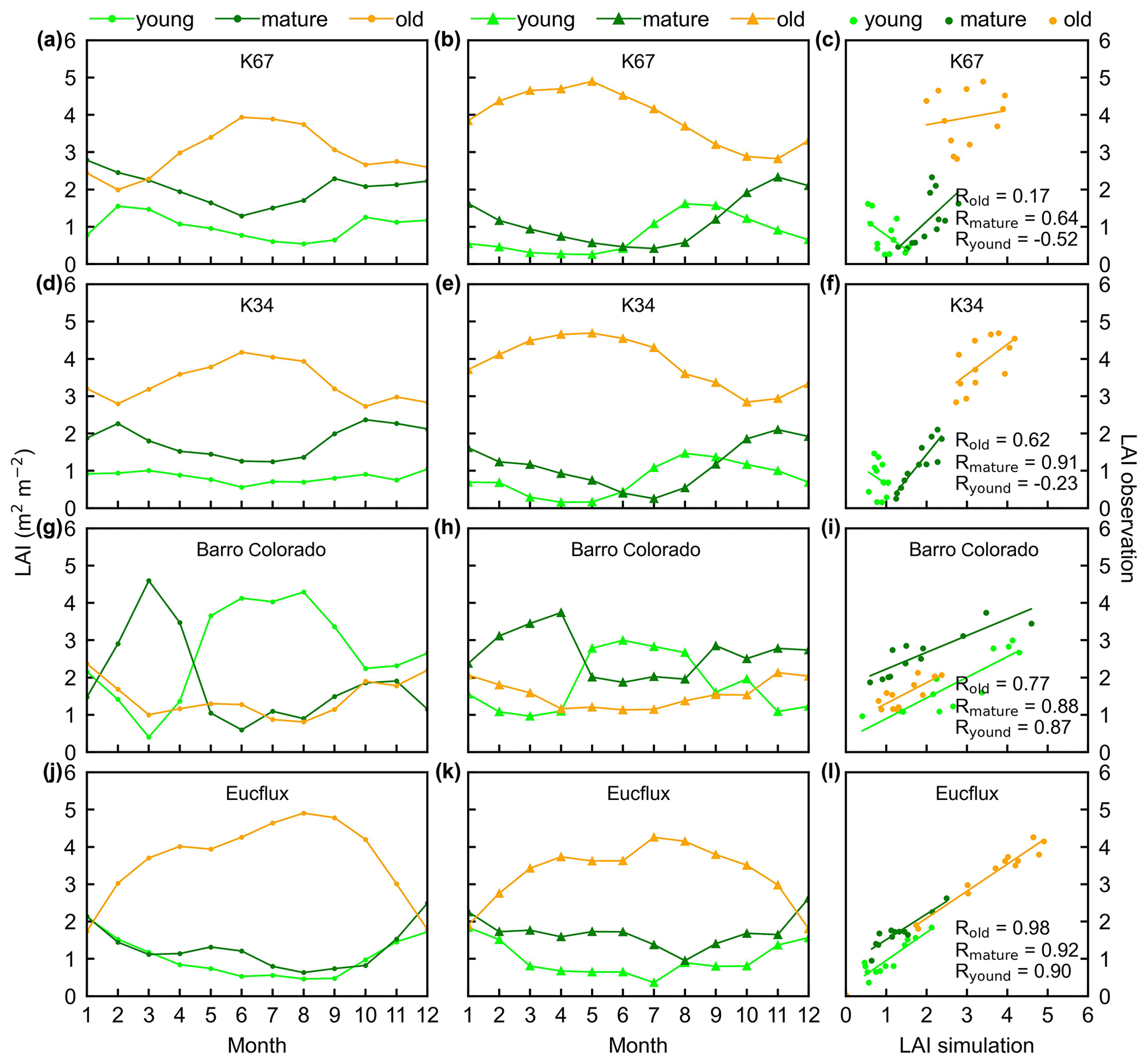
Figure 3 Seasonality of simulated LAI_young, LAI_mature, and LAI_old, in comparison with observed data at four sites in South America. (a, d, g, and j) Simulated LAIs. (b, e, h, and k) Observed LAIs. (c, f, i, and l) Scatterplots between simulated and observed LAIs. Lime green dots are LAI_young, green dots are LAI_mature, and orange dots are LAI_old.

4 Results

4.1 Comparison of LAI cohort seasonality with site observations

The simulated leaf-age-dependent LAI seasonality product was validated against the camera-based measurements of LAI_young, LAI_mature, and LAI_old at four sites in South America, one site in Congo, and three sites in China. Overall, the LAI seasonality of mature and old classes from the new Lad-LAI products agrees well at these sites, with very fine-scale collections of monthly LAI of mature (R=0.77; MSD =0.69) and old leaves (R=0.59; MSD =0.62). However, the seasonality of simulated LAI from young leaves performs poorly (R=0.36; MSD =0.45). It is also interesting to note that the canopy leaf phenology of TEFs at these sites differs greatly. In South America, at K67, K34, and EUCFLUX sites, both in situ and simulated LAI_young and LAI_mature decrease early in the dry season, around February, and convert to an increase early in wet season, around June (Fig. 3a, b, d, e, j, k). At the Barro Colorado site, LAI_young increases from the late dry to early wet season, around March, in response to the increasing incoming shortwave radiation, and in contrast, LAI_mature starts to increase in the wet season, around June (Fig. 3g, h). However, in subtropical Asia, LAI_young and LAI_mature increase during the wet season and peak with largest rainfall in June or July at the Din, Gutian, and Banna sites (Fig. 5a, b, d, e, g, h). In Congo, we only found one site (CONGOFLUX) with a 6-month observation period (from May to October). The seasonality of LAI_young and LAI_mature are similar to those in tropical Asia, while having smaller variations in magnitude due to the moderate seasonality of sunlight in the equatorial region (Fig. 4a, b). Overall, there is a reverse pattern for the LAI_old seasonality compared to LAI_mature for all eight sites.

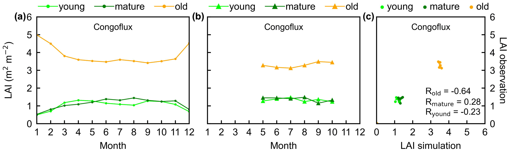
Figure 4 Seasonality of simulated LAI_young, LAI_mature, and LAI_old in comparison with observed data at one site in Congo. (a) Simulated LAIs. (b) Observed LAIs. (c) Scatterplots between simulated and observed LAIs. Lime green dots are LAI_young, green dots are LAI_mature, and orange dots are LAI_old.

Additionally, only one ground site (Barro Colorado site in Panama) had observed time series camera-based phenological imagery, which was then used to evaluate the capacity of Lad-LAI in representing the interannual dynamics of three LAI cohorts, with R values being equal to 0.54, 0.64, and 0.49 for LAI_young, LAI_mature, and LAI_old, respectively (Fig. 6). However, more in situ long-term observations are needed to test the robustness of the time series variations. The temporal variations in LAI_young, LAI_mature, and LAI_old across eight sub-regions classified by the K-means clustering analysis are shown in Fig. S6. Results showed that, for example, the LAI_mature increased significantly due to 2015 drought in the Amazon basin (e.g., sub-region S2; Fig. S6) and southeast Asia (e.g., sub-region S7; Fig. S6), indicating a good capability for detecting the dynamics of LAI_young, LAI_mature, and LAI_old in response to climate disturbances.

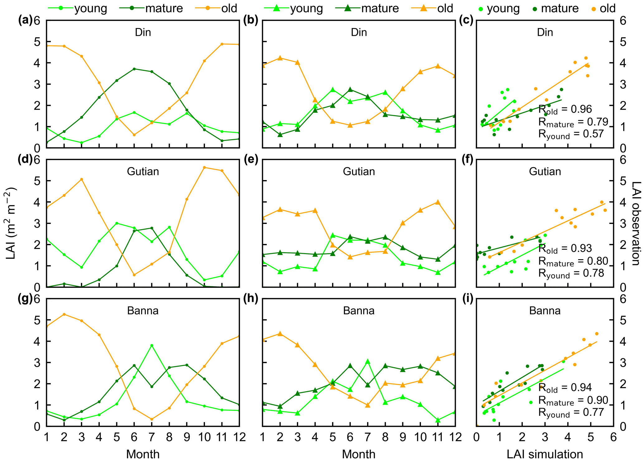
Figure 5 Seasonality of simulated LAI_young, LAI_mature, and LAI_old in comparison with observed data at three sites in tropical Asia. (a, d, g) Simulated LAIs. (b, e, h) Observed LAIs. (c, f, i) Scatterplots between simulated and observed LAIs. Lime green dots are LAI_young, green dots are LAI_mature, and orange dots are LAI_old.

4.2 Comparison of patterns of gridded LAI cohort seasonality with climatic and phenological patterns

The in situ measurements of LAI_young, LAI_mature, and LAI_old suggested diverse patterns of Lad-LAI seasonality over the TEFs. Nevertheless, the sparse coverage of these sites created challenges for a comprehensive and direct evaluation of leaf-age-dependent LAI seasonality product. To evaluate the robustness of the gridded Lad-LAI seasonality product at the regional scale, we further conducted spatial clustering analyses of LAI_young, LAI_mature, and LAI_old, using the K-means analysis method.

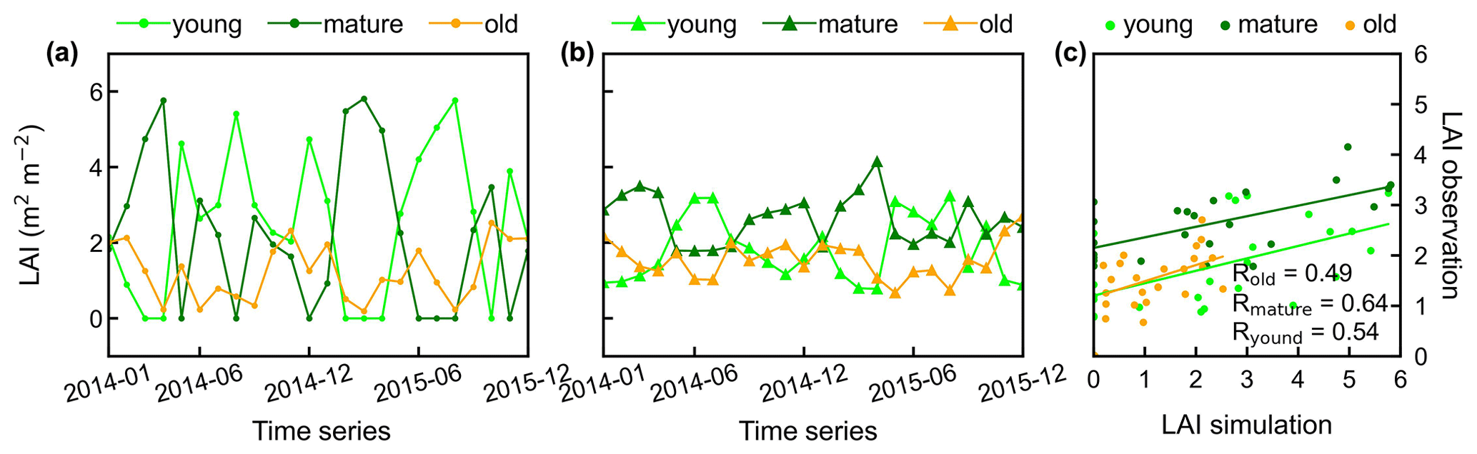
Figure 6 Time series of simulated LAI_young, LAI_mature, and LAI_old, in comparison with observed data at Barro Colorado site in Panama. (a) Simulated LAIs. (b) Observed LAIs. (c) Scatterplots between simulated and observed LAIs.

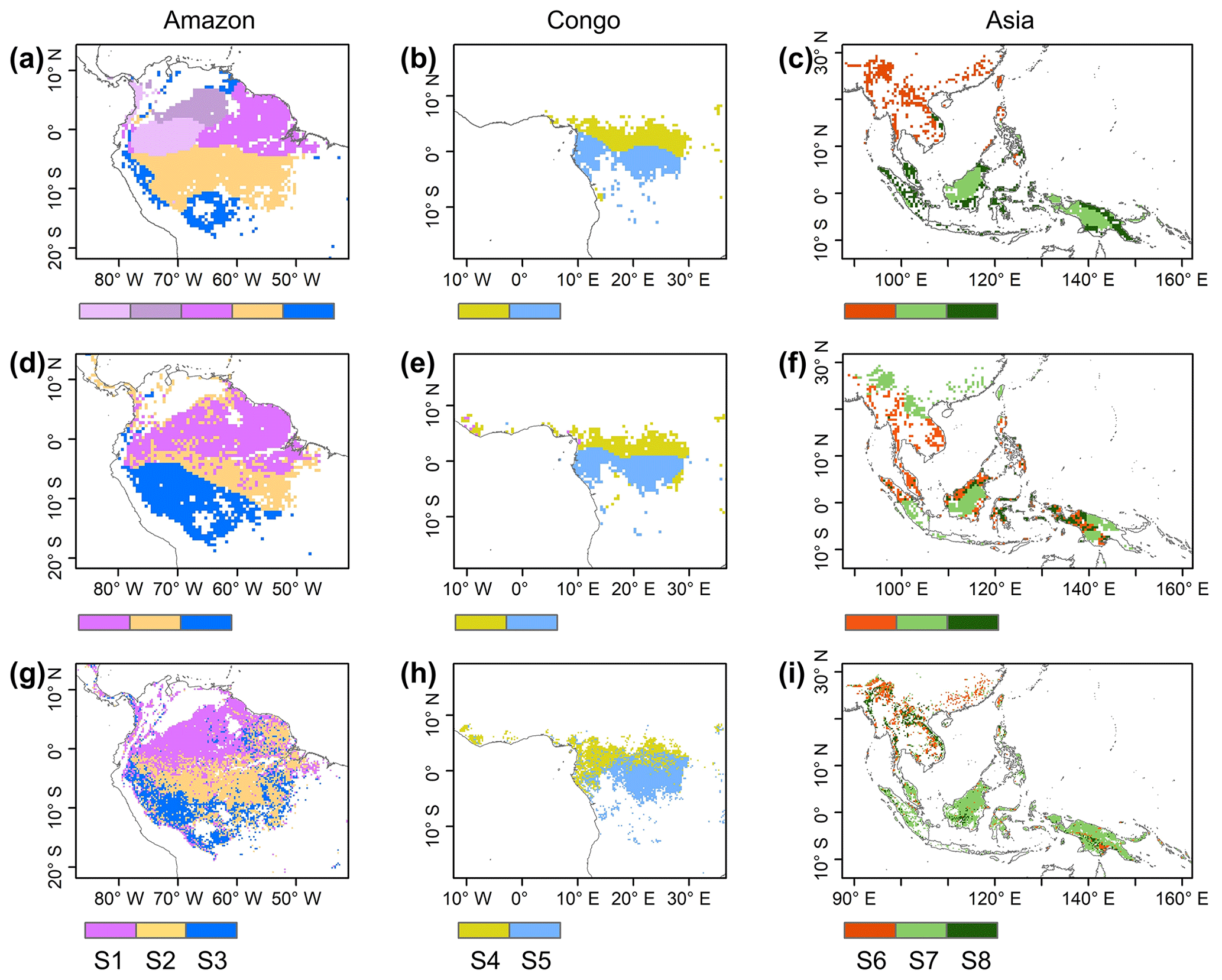
Figure 7 Comparison of sub-regions of Lad-LAI products (g–i) with those of climatic factors classified by the K-means clustering analysis (a–c), following Chen et al. (2021), and those of the three climate–phenology regimes (d–f), as developed by Yang et al. (2021).

Surprisingly, the spatial patterns of Lad-LAI product clustered from satellite-based vegetative signals (Fig. 7g–i) coincide well with those clustered from in-dependent climatic variables (rainfall, radiation, etc.; Fig. 7a–c). These patterns are also similar to those of the climate–phenology rhythms mapped by Yang et al. (2021), which suggested different correlations of litterfall seasonality with canopy phenology between different climate–phenology rhythms (Fig. 7d–f). In the central (sub-region S2) and south (sub-region S3) Amazon (Fig. 7g), the seasonality of LAI_young, LAI_mature, and LAI_old (Fig. 8b, c) are similar to those of the BR-Sa1 and BR-Sa3 sites. And in subtropical Asia (sub-region S6; Fig. 7i), the seasonality of the three LAI cohorts (Fig. 8f) are similar to those of the Din, Gutian, and Banna sites. Notably, in the sub-region S8, located geographically between sub-regions S6 and S7, LAI_young shows a peak at July, and LAI_mature shows a bimodal phenology (Fig. 8h). The remaining four sub-regions (sub-regions S1, S4, S5, and S7) are all located near the Equator. The magnitudes of seasonal changes in LAI cohorts are smaller than those in sub-regions S2, S3, S6, and S8 (away from the Equator). It is worth noting that, for these sub-regions around the Equator, there is a bimodal seasonality pattern for LAI_mature, with the first peak around March and the second peak around August (Fig. 8a, d, e, g). This is consistent with the findings of Li et al. (2021), who found that tropical and subtropical TEFs changed from a unimodal phenology at higher latitudes to a bimodal phenology at lower latitudes.

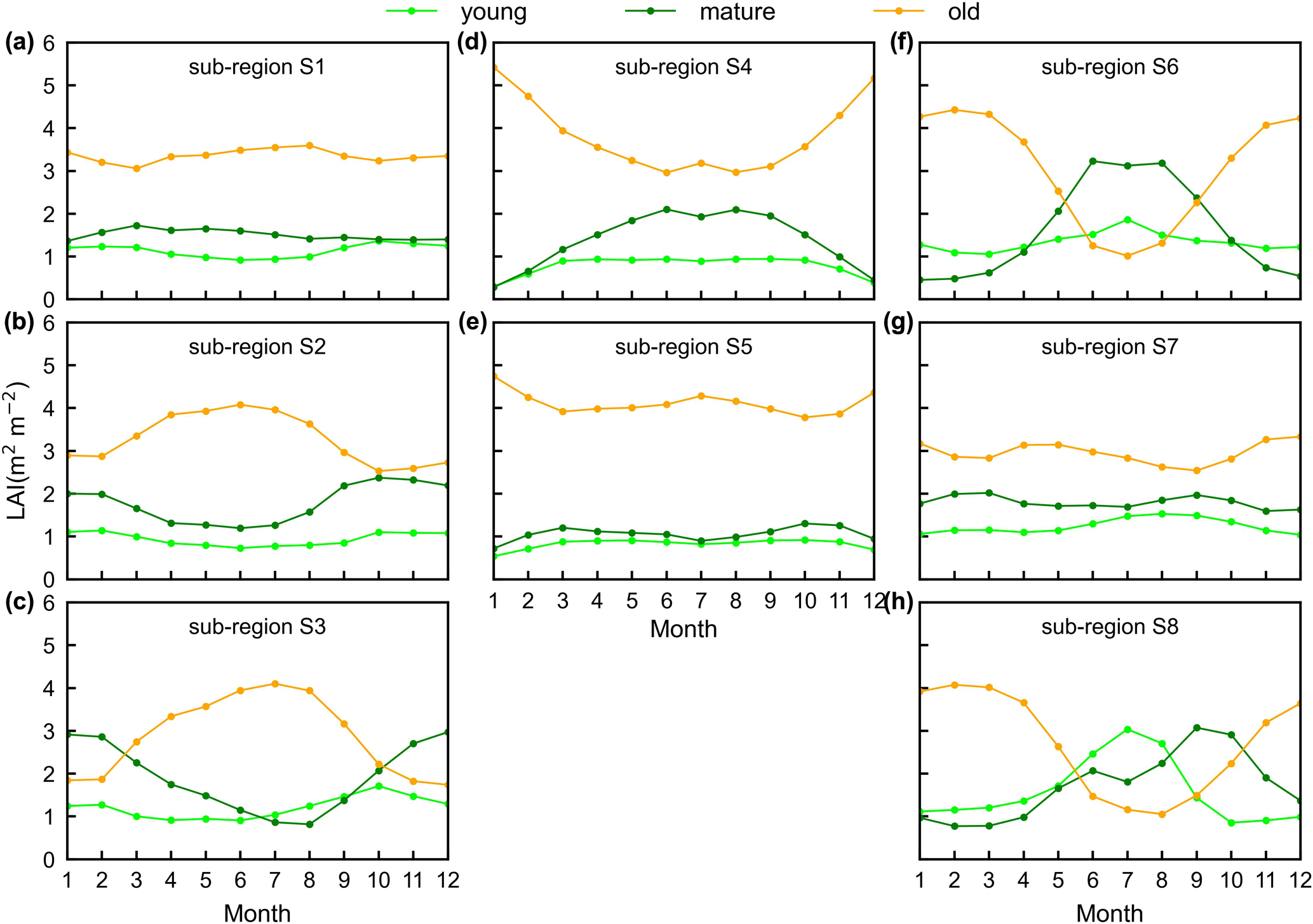
Figure 8 Seasonality of simulated LAI_young, LAI_mature, and LAI_old in eight sub-regions classified by the K-means clustering analysis.

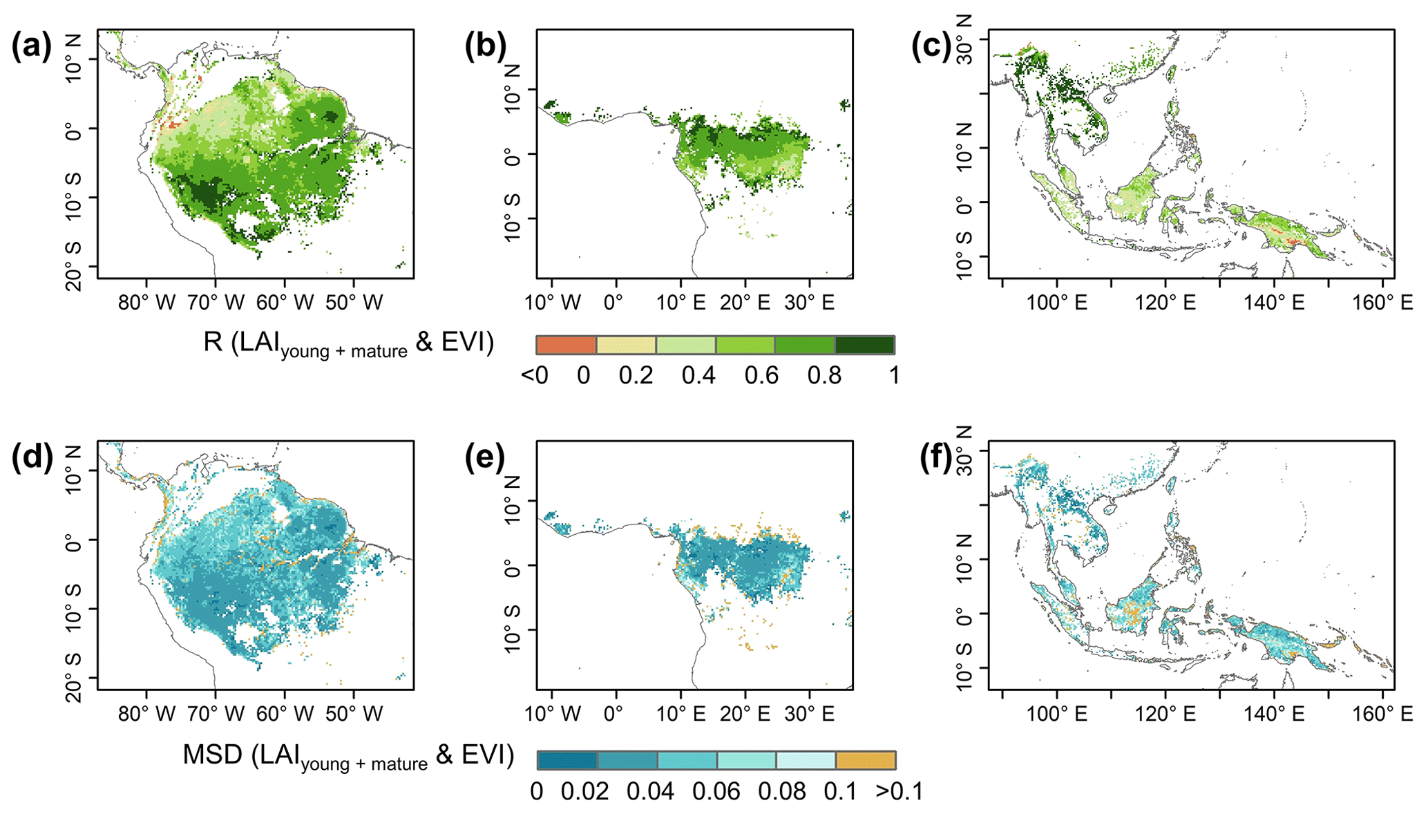
Figure 9 Pearson correlation coefficient (R) and mean squared deviation (MSD) between seasonality of the simulated LAI_young+mature and MODIS enhanced vegetation index (EVI).

4.3 Sub-regional evaluations of gridded LAI_young+mature seasonality, using satellite-based EVI products

The gridded dataset of monthly LAI_young+mature was indirectly evaluated using the satellite-based EVI products (Wang et al., 2017; de Moura et al., 2017; Xiao et al., 2005; Wu et al., 2018), as EVI was consistent with LAI_young+mature in seasonality (Figs. S7–S8), which agreed with previous findings that EVI can be considered to be a proxy for the leaf area change in those leaves with high photosynthetic efficiency (Huete et al., 2006; Lopes et al., 2016; Wu et al., 2018). This is because EVIs are very sensitive to changes in the near-infrared (NIR) reflectance (Galvão et al., 2011), while young and mature leaves also reflect more NIR signals than the older leaves they replace (Toomey et al., 2009). The linear correlation and MSD decompositions (see Sect. 3) between simulated and satellite-based EVIs are displayed in Fig. 9. Overall, the seasonal LAI_young+mature is well correlated with satellite-based EVI (R>0.40) in 78.26 % of the TEFs, and the average correlation coefficient is equal to 0.61 (Fig. 9a–c). The MSD is smaller than 0.1 in 89.69 % of the whole tropical and subtropical TEFs (Fig. 9d–f). Statistics in the eight clustered sub-regions show that the seasonal LAI_young+mature of Lad-LAI data mostly correlate better with seasonal EVI in high-latitude areas (sub-region S2 R=0.65; sub-region S3 R=0.71; sub-region S6 R=0.67) than those in low latitudes (sub-region S1 R=0.46; sub-region S5 R=0.61; sub-region S7 R=0.44; sub-region S8 R=0.64), except for sub-region S4 (R=0.72; Figs. 10, S9). The MSD components also confirm a better performance of LAI_young+mature seasonality in high-latitude areas (sub-region S2 d_bias=0.009, d_var=0.001, and d_phase=0.030; sub-region S3 d_bias=0.009, d_var=0.002, and d_phase=0.030; sub-region S6 d_bias=0.016, d_var=0.005, and d_phase=0.040) than in low-latitude areas near the Equator (sub-region S1 d_bias=0.012, d_var=0.001, and d_phase=0.041; sub-region S4 d_bias=0.020, d_var=0.001, and d_phase=0.031; sub-region S5 d_bias=0.017, d_var=0.001, and d_phase=0.032; sub-region S7 d_bias=0.018, d_var=0.002, and d_phase=0.043; sub-region S8 d_bias=0.012, d_var=0.005, and d_phase=0.035; Figs. 11, S9). This happens because the accuracy of Lad-LAI in representing the seasonality of LAI cohorts depends highly on the input SIF data, which have low sensitivity to canopy phenology and show marginally small seasonal changes nearby the Equator, for example, in tropical Asia (Guan et al., 2015, 2016).

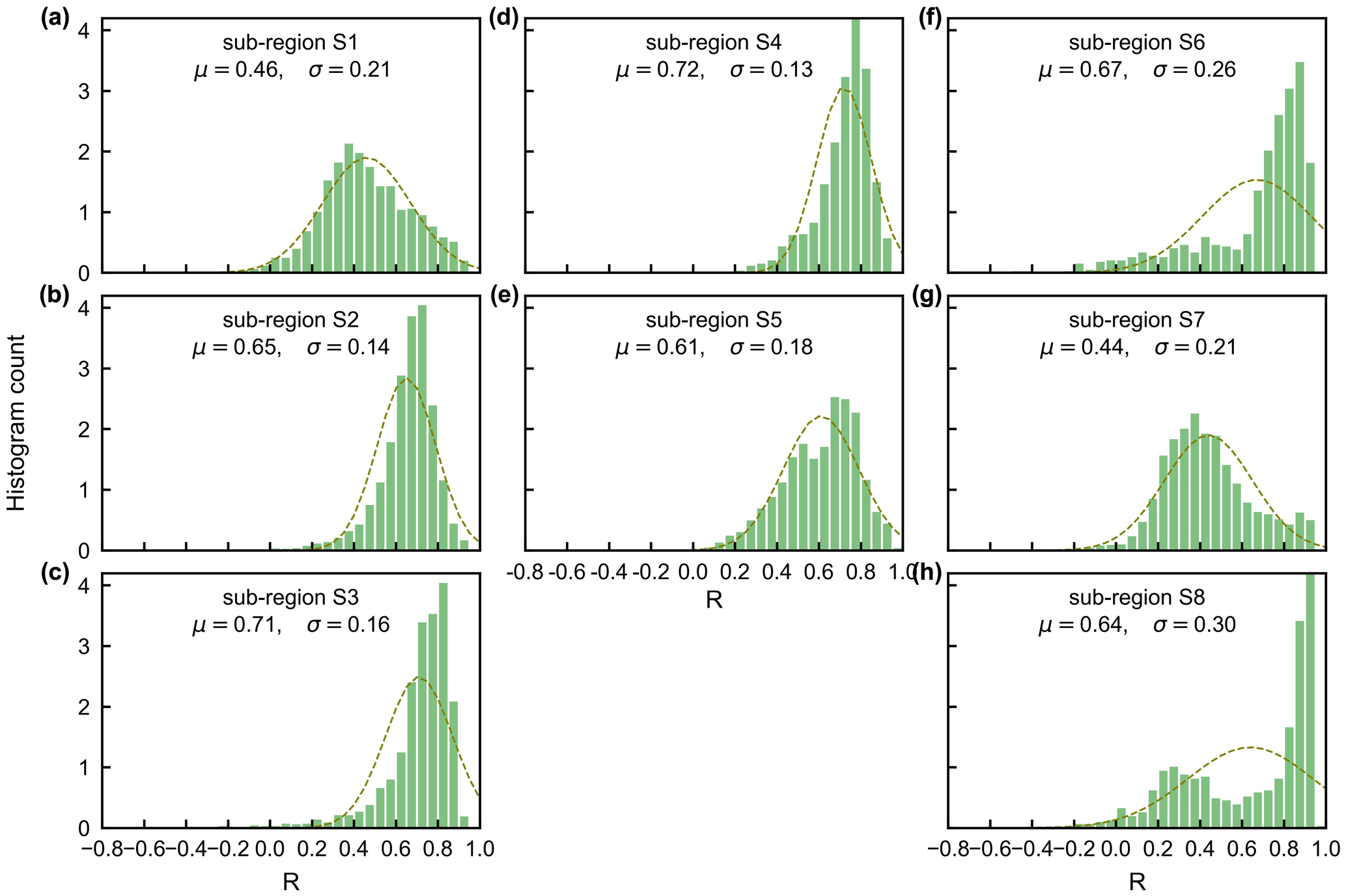
Figure 10 Statistics of the Pearson correlation coefficient (R) between the seasonality of simulated LAI_young+mature and MODIS enhanced vegetation index (EVI) in the eight clustered sub-regions.

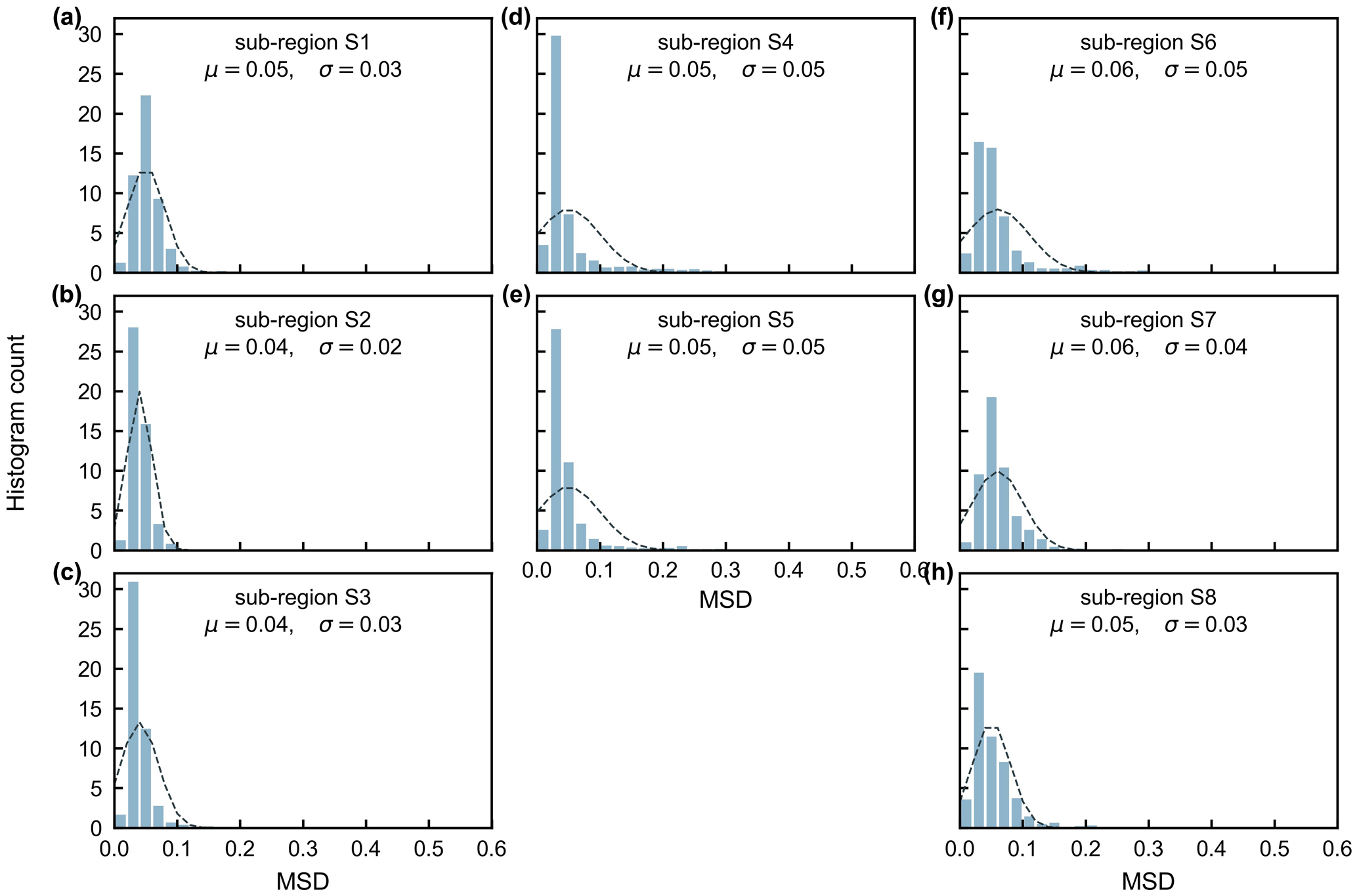
Figure 11 Statistics of the mean squared deviation (MSD) between seasonality of simulated LAI_young+mature and MODIS enhanced vegetation index (EVI) in the eight clustered sub-regions.

Additionally, previous studies indicated a large-scale green-up area over the tropical and subtropical region during the dry seasons (i.e., Guan et al., 2015; Tang and Dubayah, 2017; Myneni et al., 2007), where the average annual precipitation exceeds 2000 mm yr⁻¹. Here, we calculated the differences (Δ) between wet- and dry-season LAI_young+mature (i.e., LAI_young+ LAI_mature), to test whether the Lad-LAI can capture this green-up spatial pattern. Spatial patterns of ΔLAI_young+mature (Fig. 12) are similar than those developed by Guan et al. (2015), with higher LAI_young+mature during the dry season (blue area) in large areas north of the Equator. This indicates an emergence of new leaf flush and an increase in mature leaves, resulting in the canopy green-up phenomenon observed by previous satellite-based signals. It is interesting to note that the total areas (blue regions in Fig. 12) of this dry-season green-up shown by LAI_young+mature are smaller than those shown by SIF signals that are almost everywhere north of the Equator. That is because that new and mature leaves often have a higher photosynthetic capacity than old leaves. A slight or moderate green-up in new and mature leaves (i.e., increase in LAI_young+mature) would boost a strong increase in photosynthesis, inducing the significant green-up shown by photosynthesis-related signals (e.g., SIF data). Therefore, photosynthesis proxies likely overestimate the areas with the green-up of new leaves during the dry seasons in the real world.

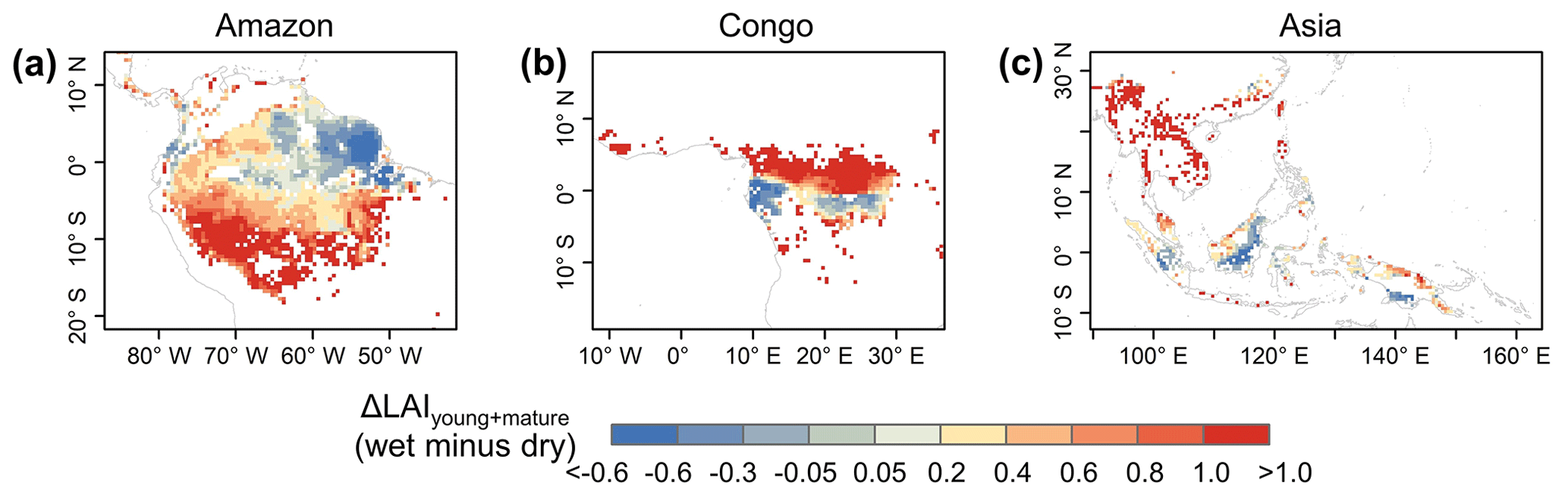
Figure 12 Spatial pattern of dry-season green-up using wet-season LAI_young+mature minus dry-season LAI_young+mature.

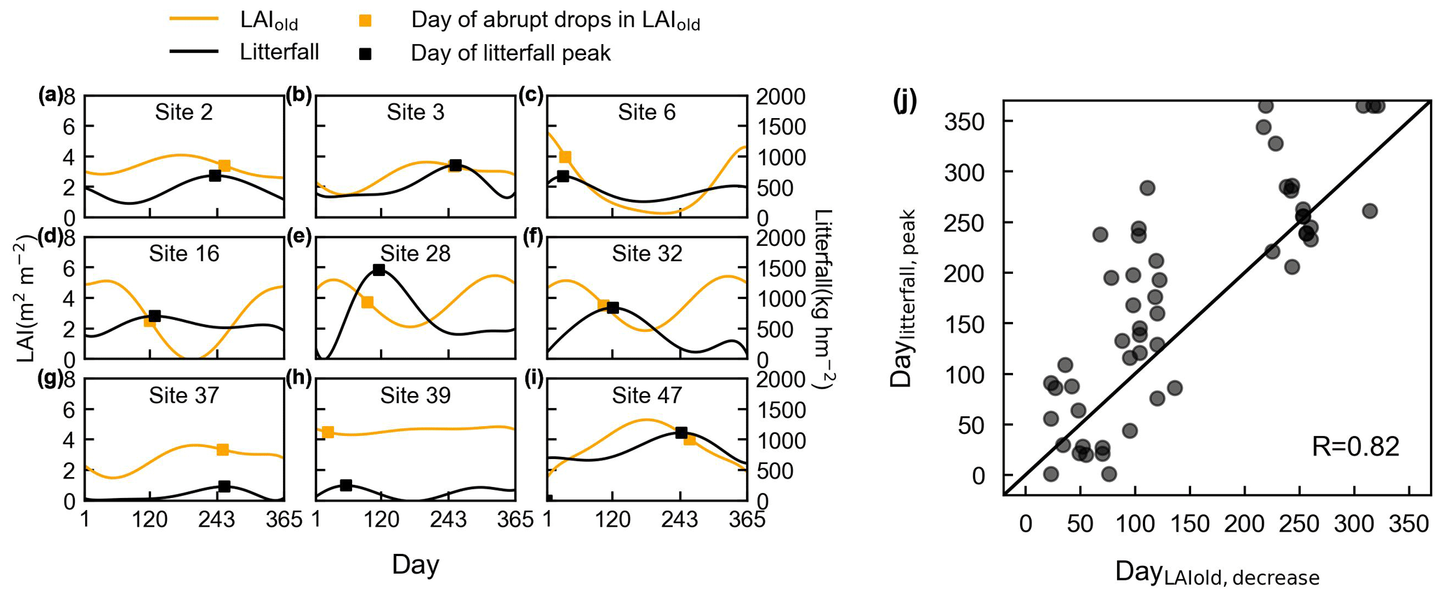
Figure 13 Evaluation of simulated LAI_old using ground-observed litterfall seasonality. (a–i) Days of an abrupt decrease in LAI_old in comparison with days of corresponding litterfall peak at nine specific sites, for example. The orange curves represent simulated LAI_old. Dots on the orange curves represent the point with an abrupt decrease in LAI_old. The black curves represent the observed seasonal litterfall mass. The dots on the black curves represent the point with litterfall peak. (j) Comparisons of the days when LAI_old has an abrupt decrease (Day_LAIold) against the days when monthly litterfall peaks (Day_litterfall).

4.4 Sub-regional evaluations of gridded LAI_old seasonality using site-based litterfall observations

The seasonal patterns of LAI_old were evaluated indirectly using ground-based seasonal litterfall observations from 53 sites over the tropical and subtropical TEFs (black circles in Figs. 1, S10–S12). Here, we selected nine specific sites (Fig. 13), with different patterns of litterfall seasonality and LAI_old seasonality, to illustrate the results of the analyses. Figure 13a–i illustrate the days on which there is an abrupt decrease in monthly LAI_old, which are close to the monthly litterfall peak. The days when LAI_old decreases the sharpest (Day_LAIold) agree well with the days on which their monthly litterfall peaks (Day_litterfall; Fig. 13j) and are mostly distributed near the diagonal lines (R=0.82). This validation from seasonal litterfall data indirectly demonstrates the robustness of the LAI_old seasonality of the Lad-LAI product.

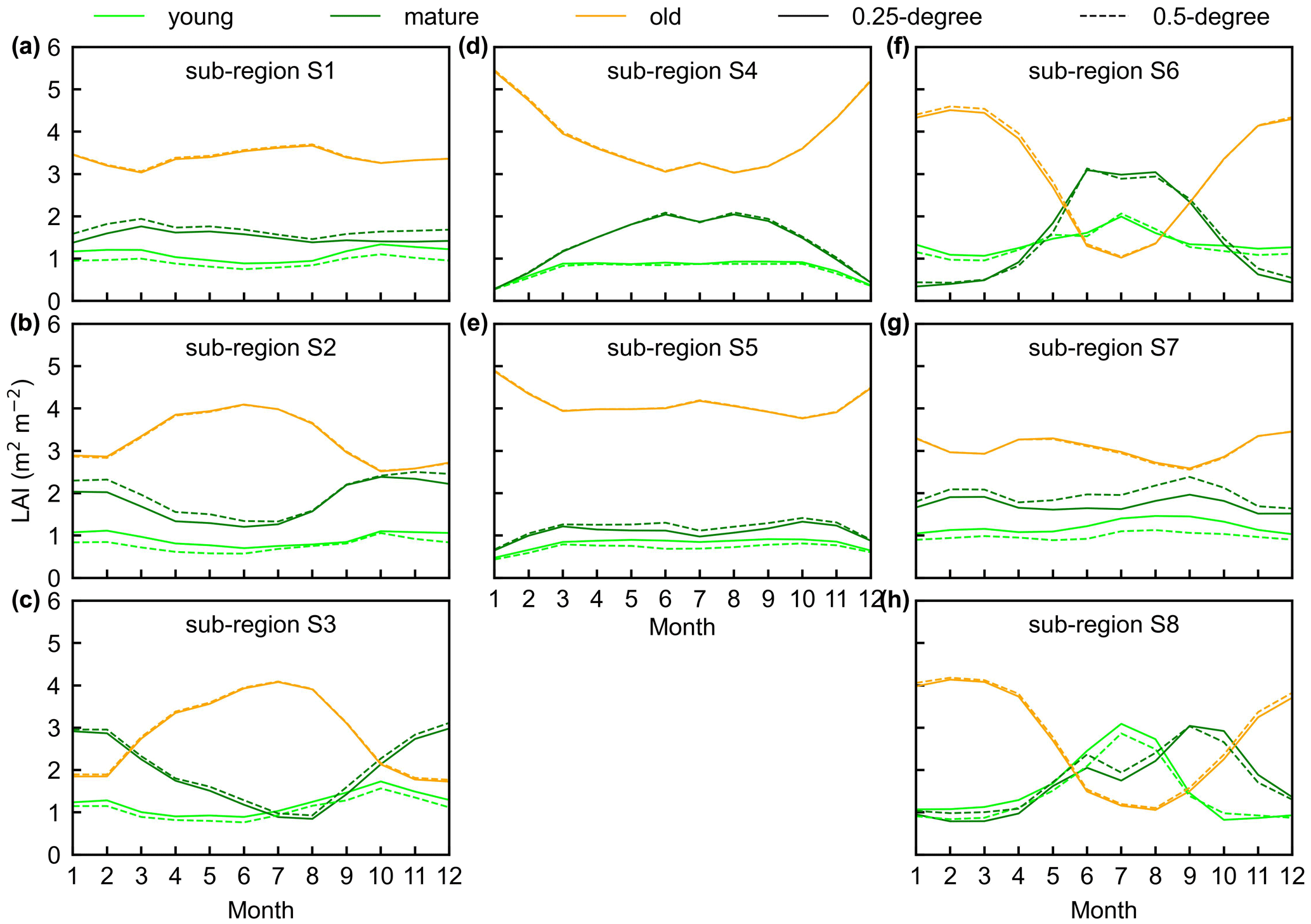
Figure 14 The seasonality of LAI_young, LAI_mature, and LAI_old between 0.25^∘ and 0.5^∘ Lad-LAI datasets in the eight clustered regions. Lime green represents LAI_young, green represents LAI_mature, and orange represents LAI_old. Solid lines represent the 0.25^∘ dataset, and the dashed lines represent the 0.5^∘ dataset.

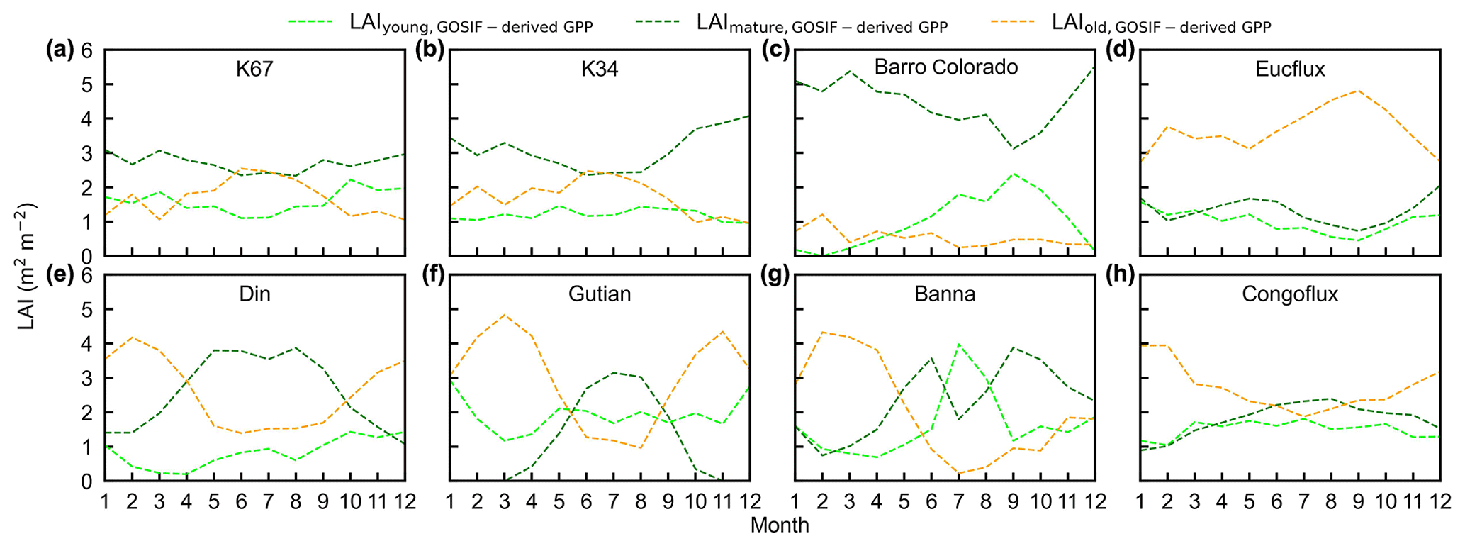
Figure 15 Seasonality of simulated LAI_young, LAI_mature, and LAI_old from GOSIF-derived GPP in comparison with observed data at eight sites. (a) K67. (b) K34. (c) Barro Colorado. (d) EUCFLUX. (e) Din. (f) Gutian. (g) Banna. (h) CONGOFLUX.

4.5 Testing potential uncertainties in the Lad-LAI products

To prove the robustness of the neighbor-based decomposition approach, we compared the Lad-LAI products generated based on 2×2 neighboring pixels with those based on 4×4 neighboring pixels. Results show that the seasonality of LAI_young, LAI_mature, and LAI_old in the 0.5^∘ Lad-LAI products based on 4×4 neighboring pixels are highly consistent with those of the 0.25^∘ one that is based on 2×2 neighboring pixels across the whole tropical region (Fig. 14), with the correlation coefficients (R) being equal to 0.63, 0.68, and 0.95, respectively (Fig. S13).

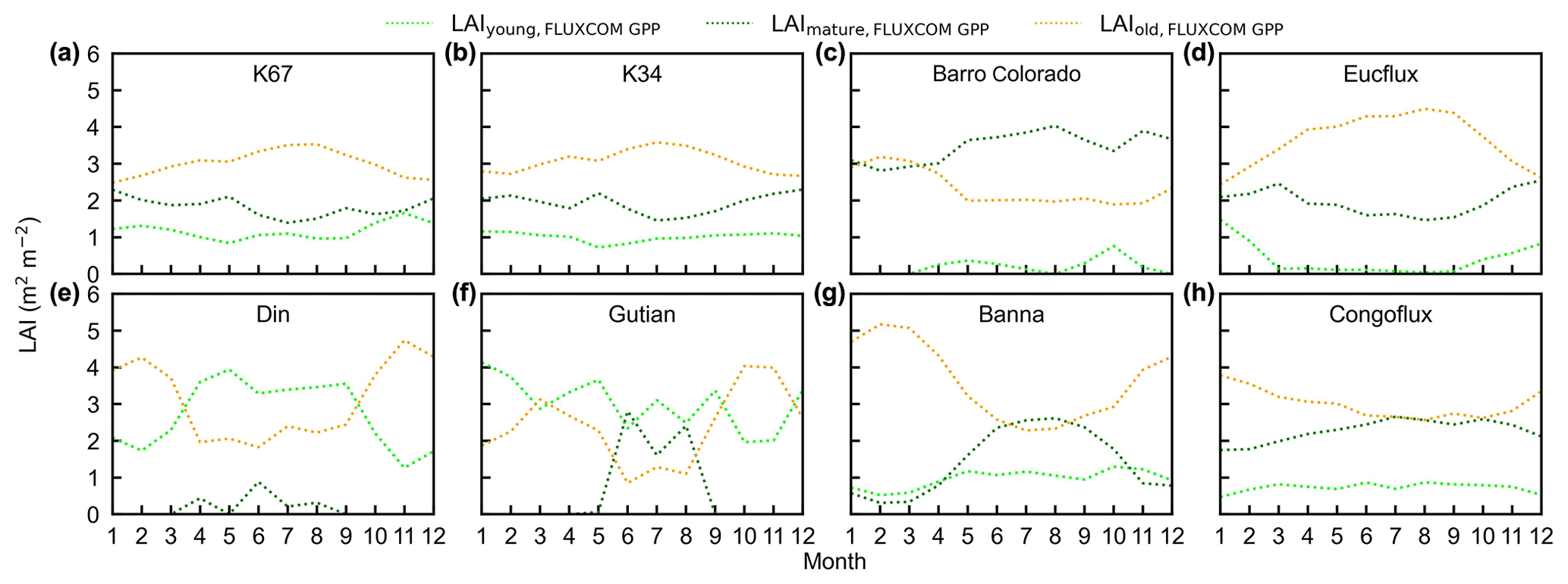
Figure 16 Seasonality of simulated LAI_young, LAI_mature, and LAI_old from the FLUXCOM GPP in comparison with observed data at eight sites. (a) K67. (b) K34. (c) Barro Colorado. (d) EUCFLUX. (e) Din. (f) Gutian. (g) Banna. (h) CONGOFLUX.

To test the uncertainties caused by the GPP estimation, we added two more GPP products, i.e., GOSIF-derived GPP (Li and Xiao, 2019) and FLUXCOM GPP (Jung et al., 2019), to produce another two versions of the Lad-LAI products. The GPP seasonality coincides well between these three data sources across all eight sub-regions (Fig. S14). By comparing them with the ground-based LAI cohorts at eight observation sites, the results show that the Lad-LAI generated from RTSIF-derived GPP show the highest correlation and a minimal deviation with the in situ measurements, with R equaling 0.36, 0.77, and 0.59 and MSD equaling 0.45, 0.69, and 0.62 for LAI_young, LAI_mature, and LAI_old, respectively (Figs. 15–16, S15–S17). Additionally, we also compared the seasonal variability in LAI_young, LAI_mature, and LAI_old between three Lad-LAI versions in eight sub-regions classified by the K-means clustering analysis (Fig. 17). In general, three versions of Lad-LAI products all performed well in eight sub-regions with a consistent seasonal variability (Fig. 17). For the regional average, sub-regions S4, S5, S6, S7, and S8 show a highly consistent seasonality of LAI_young, LAI_mature, and LAI_old between these three products, whereas the Lad-LAI generated from GOSIF-derived GPP performs a poorly in capturing the seasonality of LAI cohorts in the Amazon (sub-regions S1, S2, and S3).

5 Discussion

Leaf-age-dependent LAI performs well in describing the seasonal replacements of canopy leaves in TEFs (Wu et al., 2016; Chen et al., 2020), showing it to be a critical plant trait for representing the tropical and subtropical phenology (Doughty and Goulden, 2008; Saleska et al., 2007). However, to our knowledge, there is currently no continental-scale information of such leaf-age-dependent LAI data over the whole TEFs, as it can be neither mapped from sparse site observations (Wu et al., 2016) nor modeled from ESMs, which are triggered by unclear climatic drivers (Chen et al., 2020). These constraints hinder global researchers from accurately simulating large-scale photosynthesis (GPP) seasonality using remote sensing approaches and ESMs (Chen et al., 2020).

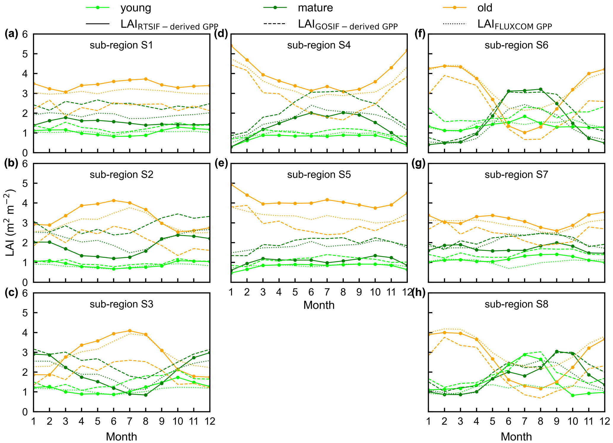
Figure 17 Seasonality of simulated LAI_young, LAI_mature, and LAI_old from three version products in eight sub-regions classified by the K-means clustering analysis. Solid lines represent LAI generated from RTSIF-derived GPP, dashed lines represent LAI generated from GOSIF-derived GPP, and dotted lines represent LAI generated from FLUXCOM GPP. Lime green represents LAI_young, green represents LAI_mature, and orange represents LAI_old.

The Lad-LAI product developed in this study is the first continental-scale gridded dataset of monthly LAI in different leaf age cohorts. Although still needing more in situ observations for an adequate validation, the seasonality of the three LAI cohorts performs well at the eight sites (four in South America, three in subtropical Asia, and one in Congo) with very fine-scale collections of monthly LAI_young, LAI_mature, and LAI_old. To test the robustness of the gridded Lad-LAI products over the whole TEFs, the seasonality of LAI_mature was also validated pixel by pixel using satellite-based EVI products, and the phases of LAI_old seasonality were compared with those of seasonal litterfall data from 53 site measurements, respectively. Moreover, the LAI_young+mature from the new Lad-LAI products can also directly represent the large-scale dry-season green-up of canopy leaves north of the Equator. Overall, direct and indirect evaluations demonstrated the robustness of the developed Lad-LAI products.

It should be noted that, over the regions with a large magnitude of annual precipitation nearby the Equator, there are no obvious dry seasons, and thus tree canopy phenology changes are smaller than higher-latitude ones throughout the year (Yang et al., 2021). The LAI of young, mature, and old leaf cohorts all show a bimodal phenology with marginally small seasonal changes near the Equator, which is captured by the developed Lad-LAI product. Second, we used a constant coefficient to transfer from SIF data to GPP and also assumed a constant value for the total LAI over the whole TEFs, which might bring additional uncertainties. This can be seen from the MSD evaluations, where the bias-related term dominates the total MSD, especially in regions near the Equator. However, this has less of an impact on the seasonality of Lad-LAI, as the phase-related term of MSD is much smaller.

Additionally, the maximum carboxylation rate (V_c,max) of leaves changes significantly with leaf age (Xu et al., 2017). Currently, most ESMs define V_c,max as a function of leaf age, whereas their relationship is still less well understood in TEFs due to sparse in situ measurements (Chen et al., 2020). This consequentially leads to the poor representation of LAI and GPP seasonality in ESMs (De Weirdt et al., 2012). To overcome this challenge, here we simplified the tree canopy into three big-leaf types (i.e., young, mature, and old) in TEFs, similar to the two big-leaf models developed for temperate and boreal forests (Best et al., 2011; Clark et al., 2011; Harper et al., 2016), which simplified the tree canopy into sun and shade leaves. However, some uncertainty remains on the assumption, as it neglects the spatial and temporal variations in V_c,max, which changes with the seasonal climate anomaly and also differs between nearby pixels in high heterogeneous forest ecosystems. This assumption may bring uncertainties for simulating seasonal An and therefore influence the seasonality of Lad-LAI.

In summary, we developed a new method to produce the first global gridded dataset for a leaf-age-dependent LAI product across the whole TEFs at the continental scale. Although some uncertainties might remain, the Lad-LAI products could provide seasonal age-dependent LAI data at the pixel level to develop a common phenology model for the whole tropical and subtropical TEFs in ESMs that are currently run at a coarser resolution. With the development of remote sensing technology, finer temporal and spatial resolutions of SIF products will enable finer temporal- and spatial-resolution maps of Lad-LAI products in the future.

6 Data availability

The 0.25^∘ leaf-age-dependent LAI seasonality (Lad-LAI) data from 2001–2018 are presented in this paper as the main dataset, and their time series are as a supplementary dataset. The two datasets are available at https://doi.org/10.6084/m9.figshare.21700955.v4 (Yang et al., 2022). Besides, we also provided another two versions of Lad-LAI generated from GOSIF-derived GPP and FLUXCOM GPP, respectively. These datasets are compressed in a GeoTiff format, with a spatial reference of WGS84. Each file in these datasets is named as follows: “LAI_{leaf age}_{spatial resolution}_{month/year-month}.tif”.

7 Conclusions

This study, for the first time, developed a continental-scale gridded dataset of monthly LAI in three leaf age cohorts from 2001–2018 RTSIF data. The LAI seasonality of young, mature, and old leaves was evaluated using in situ measurements of seasonal LAI data, satellite-based EVI, and in situ measurements of seasonal litterfall data. The evaluations from these datasets demonstrate the robustness of the seasonality of three leaf age cohorts. The new Lad-LAI products indicate diverse patterns over the whole tropical and subtropical regions. In the central and south Amazon, LAI_young and LAI_mature decrease early in the dry season, around February, and start to increase early in the wet season, around June. On the contrary, in subtropical Asia, LAI_young and LAI_mature increase during the wet season and peak with the largest rainfall volume in June or July. In regions near the Equator, the LAI cohorts show a bimodal phenology but with marginally small changes in the magnitude. The proposed method will enable us to produce finer temporal- and spatial-resolution maps of Lad-LAI products by using precise temporal- and spatial-resolution data as input. The Lad-LAI products will be helpful for diagnosing the adaption of tropical and subtropical forest to climate change and will also help improve the development of phenology models in ESMs.