the Creative Commons Attribution 4.0 License.
the Creative Commons Attribution 4.0 License.
 | 23 Jun 2023
NH-SWE: Northern Hemisphere Snow Water Equivalent dataset based on in situ snow depth time series
Adrià Fontrodona-Bach
Bettina Schaefli
Ross Woods
Adriaan J. Teuling
Joshua R. Larsen
Ground-based datasets of observed snow water equivalent (SWE) are scarce, while gridded SWE estimates from remote-sensing and climate reanalysis are unable to resolve the high spatial variability of snow on the ground. Long-term ground observations of snow depth, in combination with models that can accurately convert snow depth to SWE, can fill this observational gap. Here, we provide a new SWE dataset (NH-SWE) that encompasses 11 071 stations in the Northern Hemisphere (NH) and is available at https://doi.org/10.5281/zenodo.7515603 (Fontrodona-Bach et al., 2023). This new dataset provides daily time series of SWE, varying in length between 1 and 73 years, spanning the period 1950–2022, and covering a wide range of snow climates including many mountainous regions. At each station, observed snow depth was converted to SWE using an established snow-depth-to-SWE conversion model, with excellent model performance using regionalised parameters based on climate variables. The accuracy of the model after parameter regionalisation is comparable to that of the calibrated model. The key advantages and strengths of the regionalised model presented here are its transferability across climates and the high performance in modelling daily SWE dynamics in terms of peak SWE, total snowmelt and duration of the melt season, as assessed here against a comparison model. This dataset is particularly useful for studies that require accurate time series of SWE dynamics, timing of snowmelt onset, and snowmelt totals and duration. It can, for example, be used for climate change impact analyses, water resources assessment and management, validation of remote sensing of snow, hydrological modelling, and snow data assimilation into climate models.
- Article
(10384 KB) - Full-text XML
- BibTeX
- EndNote


The modification of the cryosphere is one of the most visible effects of ongoing climate warming (Beniston et al., 2018). In this context, snow cover is particularly important, as it provides an important seasonal hydrologic buffer over high latitudes and high elevations, through storage over the accumulation season and a delayed release of water in the subsequent melt season (Kuppel et al., 2017). Snow cover also plays an important role in the Earth's climate through snow–albedo feedbacks (Déry and Brown, 2007). Studies showing the impact of global warming on snow are numerous: declining trends in snow depth have been observed over the European Alps (Matiu et al., 2021a), the Pyrenees (López-Moreno et al., 2020), and all of Europe except the coldest climates (Fontrodona Bach et al., 2018); decreasing snow cover duration and extent have been reported over the Northern Hemisphere (Bormann et al., 2018; Mudryk et al., 2020) and over 78 % of global mountain regions (Notarnicola, 2020); and increasing snowmelt in winter has been observed in western North America (Musselman et al., 2021). Regions whose water resources strongly depend on snow water storage are at risk of large declines in spring and summer streamflow, posing a potential future threat to human water used for ∼2 billion people (Mankin et al., 2015). There is therefore an ongoing need for access to wide coverage and reliable snow data and research.
There are various ways to measure snow, which serve different scientific purposes. Snow depth is the thickness of snow accumulated above ground level and can easily be measured manually with a ruler or automatically with an acoustic sensor that measures snow height. The depth of water that is actually stored in a snowpack is referred to as snow water equivalent (SWE) and corresponds to the depth of liquid water that would result from melting the entire snowpack.
Reliable estimates of SWE, rather than snow depth, are thus needed for water resources assessments across scales. However, limitations arise when estimating SWE at regional, continental or global scales. Remote sensing estimates of SWE provided by satellite measurements are in constant development but currently have low accuracy and are limited to shallow (<150 mm) snowpacks (Luojus et al., 2021). Estimates of SWE resulting from reanalysis and land surface modelling rely on snow models forced with meteorological data and are also subject to biases and errors (Brun et al., 2013; Broxton et al., 2016; Muñoz-Sabater et al., 2021). A common limitation of these gridded SWE estimates is that they cannot reproduce the high spatial variability of snow on the ground, especially for mountain regions and complex terrain (Clark et al., 2011; López-Moreno et al., 2013), although reliability and resolution can be improved by assimilating measurements of snow depth and SWE (Zeng et al., 2018). A review of global gridded datasets of SWE shows up to a 50 % variability in peak snow accumulation between different datasets (Mudryk et al., 2015).
Adding to the complexity of obtaining reliable SWE data, large-scale estimates of SWE often have limited validation against observed ground data, which is scarce in time and in space. In fact, both manual and remotely sensed measurement techniques exist for SWE, but they are either complex, time consuming or require specialised equipment (Jonas et al., 2009; Winkler et al., 2021). In contrast to complex SWE measurements, manual and automatic snow depth measurements are more straightforward and therefore more widespread. Many regional snow depth datasets exist or are emerging, with an increasing number of national hydrological and meteorological services making snow depth data publicly available and easily downloadable through site portals and application programming interfaces (APIs). However, an estimate of snow density is needed together with a snow depth measurement to obtain the snow water equivalent.
There is an increasing number of models that can accurately convert snow depth to SWE using simple empirical regressions (Mizukami and Perica, 2008; Jonas et al., 2009; Sturm et al., 2010; Bormann et al., 2013; Mccreight and Small, 2014; Pistocchi, 2016; Hill et al., 2019; Ntokas et al., 2021). These regression-based methods require paired snow depth–SWE ground measurements to calibrate parameters that later on are used to estimate SWE when only snow depth measurements are available. Some of the approaches generalise parameters regionally, based on elevation and on the day of the year (Jonas et al., 2009), or globally based on climatological variables (Sturm et al., 2010; Hill et al., 2019; Szeitz and Moore, 2023). Physics-based snow models can also regionalise and cluster snow parameters based on climate variables (Dawson et al., 2017; Sun et al., 2019, 2022), but the parameterisation is more data intensive than for simple regression-based approaches. The common limitation of using regression-based approaches is that a SWE value on a given time step is estimated independently for each snow depth value, irrespective of snow depth values on preceding time steps. Therefore, conversion of time series of snow depth to SWE leads to an incorrect temporal evolution of SWE, because the regression cannot account for the settling of new snow nor for the compaction of the snowpack (Jonas et al., 2009). This problem has been addressed by considering the temporal evolution of snow depth in the conversion model (Mccreight and Small, 2014; Winkler et al., 2021), but, to date, no approach has generalised this method for regional or global use.
Here we bring together the increasing number of available in situ snow depth datasets and the increasing number of snow depth to SWE conversion models to produce a new, freely available SWE dataset: the NH-SWE dataset. This compilation and analysis provides (i) the first pan-Northern Hemisphere in situ snow depth time series compilation and (ii) a conversion from depth to SWE using an established model (ΔSNOW; Winkler et al., 2021). This SWE dataset can be extremely useful across a wide variety of applications such as validation of remote sensing products, hydrological and environmental modelling, assimilating snow data into models, and general climate research.
This paper is organised as follows: (1) we show data sources used to calibrate, regionalise, and evaluate the model for snow depth to SWE conversion (Sect. 2); (2) model development and implementation (Sect. 3); (3) performance of the model across a variety of variables (Sect. 4); and (4) demonstration of some key features of the NH-SWE dataset (Sect. 5), including its usage and limitations (Sect. 6).
The data used to compile NH-SWE from in situ snow depth observations can be divided into two main groups: group HS-SWE includes all stations that have both snow depth (height of snow, HS) and SWE data available; group HS includes all stations that have only HS observations available.
Group HS-SWE data can be further split for the purposes of model implementation into (a) data used for model regionalisation and (b) data used for independent evaluation. The HS data group then provides the input data to generate the new SWE estimates within the NH-SWE dataset (Sect. 5) but is not used in model implementation. We evaluate the model using independent HS-SWE datasets, different from the one used to regionalise the ΔSNOW model from Winkler et al. (2021). This approach enables us to evaluate SWE estimates for as wide a range of snow climate conditions as possible combined with an independent evaluation process to test the transferability of the model regionalisation to other independent datasets, such as our collection of Northern Hemisphere snow depth time series. A summary chart of the workflow to produce the final SWE dataset is shown in Fig. 1. An overview of all the data used to derive the NH-SWE dataset is shown in Table 1, and the spatial distribution of the data and sources is shown in Fig. 2.
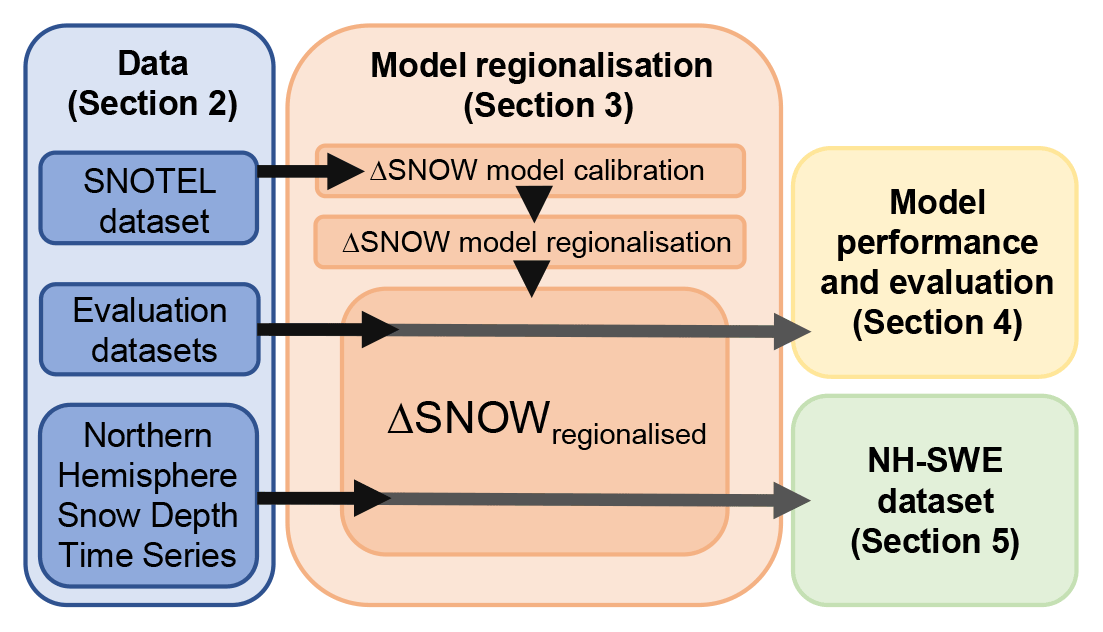
Figure 1Workflow chart to obtain the NH-SWE dataset. The ΔSNOW model is from Winkler et al. (2021).
2.1 HS-SWE data for model regionalisation
The SNOwpack TELemetry Network (SNOTEL) dataset contains a large network of automated sub-daily observations of HS and SWE data over the western United States and is freely available (USDA NRCS, 2022). The dataset covers a wide range of snow climates and characteristics such as the wet and mild Pacific Northwest (including the maritime Cascades mountain range), the continental cold and snowy Rockies, the Mediterranean climate from California, the arid climate from the southwest, and even high-latitude tundra/taiga in Alaska (Serreze et al., 1999; Sun et al., 2019). The SNOTEL dataset only contains measurement stations where a minimum of 40 d of continuous snow cover is observed on average (since it has been designed to monitor seasonal snowpacks). We use this dataset to calibrate and regionalise the ΔSNOW model (Winkler et al., 2021) over a wide range of hydroclimates, and we assess the transferability of the regionalisation by evaluating the model over fully independent datasets from other climates. We apply the same data preprocessing to the SNOTEL dataset as Hill et al. (2019), retaining only measurement stations with joint HS and SWE records and removing outliers. The resulting dataset for model regionalisation contains 812 sites with daily HS-SWE time series data ranging from 1 to 25 years in length (see Table 1 and Fig. 2a).
USDA NRCS (2022)Vionnet et al. (2021, 2022)Marty (2020)RIHMI-WDC (2022)NVE (2022)Krajči et al. (2017)Essery et al. (2016)Morin et al. (2012)Stähli (2018)Klein Tank et al. (2002)FMI (2022)Matiu et al. (2021b, a)RIHMI-WDC (2022)Menne et al. (2012)MeteoSwiss (2022)Table 1Overview of datasets and sources used for model regionalisation, model evaluation and input for the final NH-SWE dataset. Model regionalisation and model evaluation data refer to Sect. 2.1 and 2.2, and input data refers to Sect. 2.3. SWEd for daily measurements, SWEb for biweekly measurements. The number of sites is after quality control and selection. The minimum length is 1 year for all datasets.
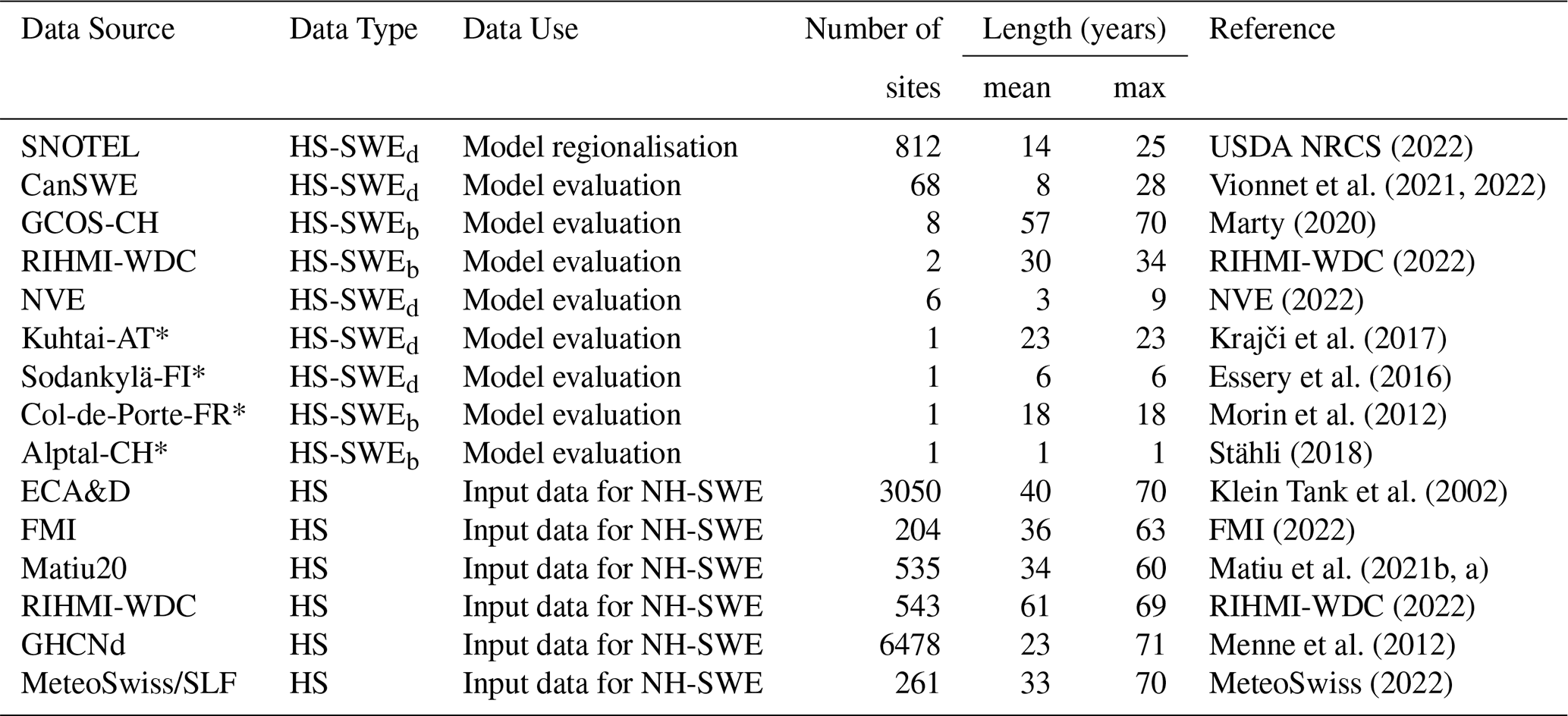
* Referred to as “single sites” in Fig. 2a
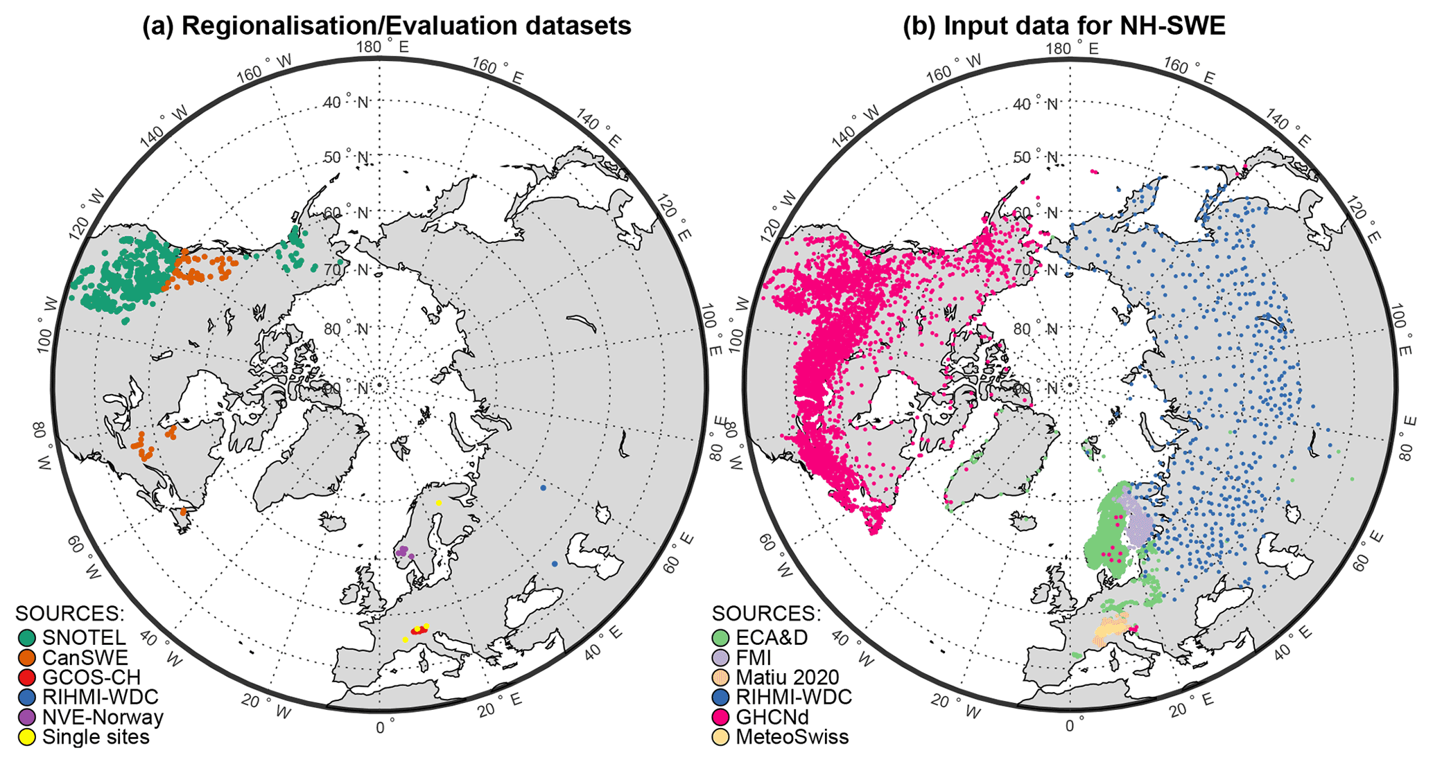
Figure 2Spatial distribution of stations in the datasets used. (a) Paired HS-SWE datasets for model regionalisation and evaluation and (b) HS data used as model input for the final modelled SWE dataset (NH-SWE). In (a), SNOTEL is used for model regionalisation, and the rest are evaluation datasets. See Table 1 for more information on the sources.
2.2 HS-SWE data for model evaluation
We independently evaluate the ΔSNOW model using a SWE dataset from Canada (Vionnet et al., 2021), which contains 2607 stations with historical HS and SWE measurements. Selecting only those stations with daily observations of HS and SWE, and applying gap-filling and quality control (see Appendix A), 68 stations distributed over eastern and western Canada are retained for model evaluation (see Fig. 2a and Table 1).
To assess the transferability of the model to outside North America, we compiled 20 additional HS and SWE datasets from seven different sources: 8 stations from the Global Climate Observing System (GCOS) in Switzerland (Marty, 2020); 2 stations from the All-Russia Research Institute of Hydrometeorological Information – World Data Center (RIHMI-WDC, 2022); 6 stations from the Norwegian Water Resources and Energy Directorate (NVE, 2022); and 4 single-station observations from different sources over the European Alps and Finland (Stähli, 2018; Krajči et al., 2017; Essery et al., 2016; Morin et al., 2012). The number of additional stations available for independent validation outside North America is low because (1) continuous observation of both HS and SWE is much rarer and (2) if collected is also rarely provided within open-data repositories. Most of this additional validation data contain daily observations of SWE, but some contain only weekly or biweekly measurements (see Table 1). This change in temporal resolution in turn reduces the metrics that can be evaluated. For example, the timing of snowmelt onset cannot be accurately determined without daily SWE measurements (see Sect. 3.6). Furthermore, the daily observations of SWE were obtained automatically and are typically co-located with the snow depth measurements. However, the biweekly SWE measurements are usually acquired through manual profiles, a destructive method that may introduce spatial variability in the measurements due to differences in the location of sampling relative to the HS data, which are typically obtained from fixed installed stakes, snow courses or automatic snow depth measurements.
2.3 HS data as model input for the NH-SWE dataset
We have gathered and compiled pan-Northern Hemisphere datasets of in situ daily HS observations from different sources. This relies on the European Climate Assessment and Dataset (ECA&D), which has already been described (Klein Tank et al., 2002) and analysed in previous studies (Fontrodona Bach et al., 2018), but with some important additions and updates. Gaps in time series from Finland in the ECA&D have been filled where possible by downloading HS time series directly from the Finnish Meteorological Institute (FMI). The underrepresentation of alpine sites in the ECA&D has been reduced through data obtained from the MeteoSwiss data portal IDAWEB, which includes data from MeteoSwiss, the SLF (WSL Institute for Snow and Avalanche Research) and the Autonomous Province of Bolzano – Südtirol. We have also included alpine data published by Matiu et al. (2021a, b). The ECA&D coverage over Russia has been completely replaced by data from the All-Russia Research Institute of Hydrometeorological Information – World Data Center (RIHMI-WDC), which contains longer and updated coverage of many sites. The western half of the Northern Hemisphere is well covered by data available from the Global Historical Climatology Network daily (GHCNd) dataset. In the case of multiple time series from the same location being available across the compiled datasets, we selected the time series with the most updated record or the one with fewer gaps. Because of the sharp increase in data availability and quality after 1950 (Fontrodona Bach et al., 2018; Matiu et al., 2021a), our data compilation begins from 1 September 1949 to 31 August 2022. Most snow depth measurements are manual with a precision of ±1 cm, but automatic measurements with higher precision are also present. Due to the large amount of data gathered, we do not provide information on the type of measurements for each snow depth dataset.
Following this initial compilation, we obtain 21 502 individual time series of snow depth, upon which we apply further selection criteria before further use. The ΔSNOW model (Winkler et al., 2021) requires a gap-free record of daily snow depth. Therefore, we use a robust gap-filling procedure to the HS time series (see Appendix A). We quality control the gap-filling based on confidence criteria and we select stations with at least one entire gap-free snow year between 1950 and 2022. We define a snow year from 1 September to 31 August, since this was the first day of the month with most snow-free records over the entire dataset. Furthermore, the ΔSNOW model can only be reliably applied over seasonal snowpacks (Winkler et al., 2021), and the SNOTEL dataset (used here for model regionalisation) contains only sites with a minimum of 40 d of continuous snow cover. Because of the uncertainty in model performance for shorter snow cover durations, we retain only stations where the mean continuous snow cover duration is at least 40 d. The number of stations in the dataset after quality control and selection criteria is 11 071. An overview of the datasets and sources is available in Table 1, and the spatial coverage is shown in Fig. 2b.
We are not allowed to republish the original HS data used as source to derive the SWE dataset because it is already freely available (See references in Table 1). More information on the data sources and how to download the HS data can be found in the “Code and data availability” section.
3.1 Definitions
We show in Fig. 3 the terms to describe the snow season. The day count of a snow year starts on 1 September, which is day 1. The annual snow season is the longest period of continuous snow cover (SWE >0 mm) in a snow year. The maximum snow water equivalent value in the annual snow season is the peak SWE. For biweekly SWE measurements, peak SWE is the highest observed SWE and is compared with the modelled SWE on the same date for the purpose of model evaluation. The value of peak SWE can last for days while there is no more snow accumulation, until the snowpack starts to melt. Snowmelt is defined as a decrease in SWE. The timing of snowmelt onset corresponds to the last day of peak SWE and divides the annual snow season into the accumulation season and the snowmelt season. Snow seasons can have more complicated accumulation and melt patterns than the one in Fig. 3, for instance if peak SWE occurs very early in the season, followed by a long cold period without a decrease in SWE. However, for computing snowmelt volume and duration, we only use days with a decrease in SWE, and thus the results should not be heavily affected by our definitions.
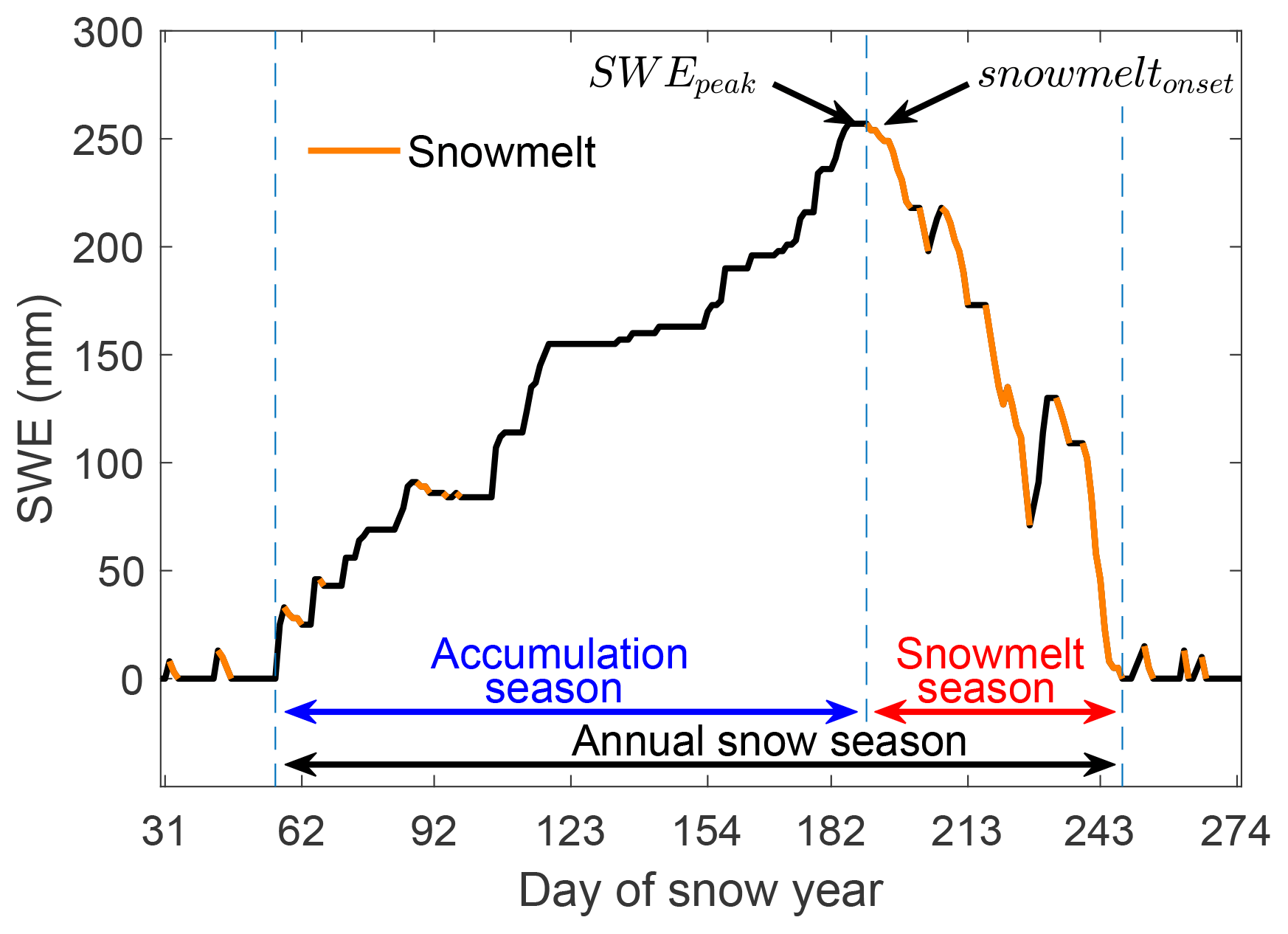
Figure 3Snow season terms and definitions. SWEpeak is the highest snow water equivalent value. Snowmelt onset is the last day of peak SWE and divides the snow season into accumulation season and snowmelt season.
3.2 Model choice and brief description
We use the ΔSNOW model of Winkler et al. (2021) to convert snow depth (HS) to snow water equivalent (SWE) time series. We use the ΔSNOW model because of its low complexity and little input data required, given that most snow depth time series do not contain other meteorological data (see Sect. 2). Furthermore, the ΔSNOW model shows a high accuracy compared to other conversion models (Winkler et al., 2021), especially because of its ability to integrate the temporal evolution of snow depth into the model. Here, we further test its ability to accurately model the temporal dynamics of SWE by evaluating the model performance on other variables (see Sect. 3.6) than simulated daily SWE and simulated peak SWE, which were the main evaluated variables in previous studies (Hill et al., 2019; Winkler et al., 2021). In addition, the low number of required parameters makes it possible to regionalise the model and to transfer it to different types of snowpacks and climates, as shown in Sect. 3.4.
The model estimates total snowpack SWE by accumulating, compacting and drenching a series of snow layers, based on the temporal evolution of snow depth and 7 parameters that need to be calibrated. The model has four modules for HS computation, which are activated according to the value of ΔHS(t) (the change in depth of the entire snow pack between t−1 and t), the density of the snow layers (ρl, which can reach a maximum density of ρmax) and a threshold deviation parameter (τ). The four modules are
-
new snow and overburden module, activated if ΔHS(t)>τ;
-
dry compaction module, activated at every time step if ρlj<ρmax for at least one snow layer j;
-
drenching module if and runoff submodule when ρl=ρmax for all snow layers;
-
scaling module when .
Each increase in snow depth activates the new snow module and creates a new layer in the snowpack. The parameter new snow density (ρ0) determines the density of the new layer. In case the snowpack already contains one or more layers, the overburden submodule is activated, which increases the density in underlying snow layers due to the weight of the new snow. The overburden parameters (kov, cov) control this submodule. There is no maximum number of snow layers, and their thicknesses are determined by the temporal evolution of snow depth.
A snow accumulation event is generally followed by a decrease in snow depth due to snow metamorphism. This process densifies the snowpack but does not imply a decrease of SWE. This densification of snow layers is computed by the dry compaction module and occurs at every time step until all layers in the snowpack reach the maximum snow density (ρmax). The densification is controlled by the viscosity parameters (η0 , k).
A decrease in snow depth also activates the drenching module, which simulates wet metamorphism and snowpack water percolation from the top to the bottom layers, further densifying the snowpack layers until all layers have reached ρmax. During dry compaction and drenching, SWE does not decrease even though snow depth does. When all layers have reached the maximum snow density, the runoff submodule is activated, and a decrease in snow depth leads to a decrease in SWE (i.e. snowmelt).
The scaling module intervenes when and avoids excessive mass loss or mass gain from uncertainties in manual and automatic snow depth measurements. When , the model re-evaluates dry compaction and makes small adjustments to HS within threshold deviation τ. For further details on the model, we refer the reader to Winkler et al. (2021).
3.3 ΔSNOW model calibration
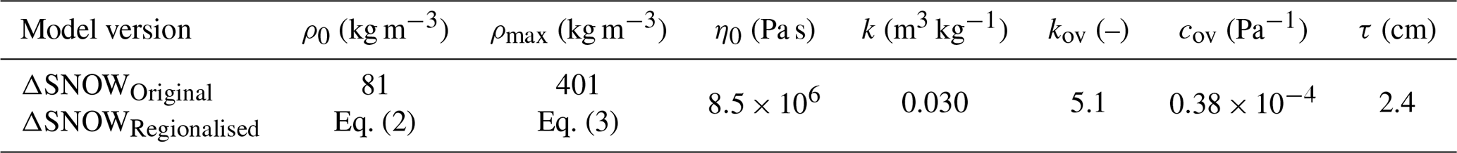
The ΔSNOW model (Winkler et al., 2021) contains seven parameters that might be site-specific or depend on local conditions. The model was originally developed and calibrated over 15 alpine sites in the Swiss and Austrian Alps with continuous measurements of snow depth (HS) and biweekly measurements of SWE. One unique set of optimised parameters was obtained by Winkler et al. (2021) for the European Alps only (Table 2). Here we use continuous time series of daily HS and SWE from 812 sites from the SNOTEL dataset (see Sect. 2.1) to calibrate the model, and we obtain one set of optimised parameters per site.
The new snow density (ρ0) is the most sensitive model parameter, largely controlling the bias in daily SWE and peak SWE (Winkler et al., 2021). Our initial tests showed that the maximum snow density (ρmax) has a stronger impact on the timing of modelled peak SWE than on the modelled daily SWE, a sensitivity which was not explicitly tested in the work of Winkler et al. (2021). This sensitivity is not surprising, because the maximum snow density determines the maximum densification of the snowpack, after which any decrease in snow depth will lead to a decrease in SWE. However, the magnitude of modelled peak SWE is still mostly controlled by the new snow density parameter. Even though Winkler et al. (2021) suggest calibration of all seven parameters of the model, our tests showed that ρ0 and ρmax are the only two parameters that exhibit some relationship with the climate variables that we used (see Sect. 3.4). Therefore, we focus here on the calibration of these two key parameters, ρ0 and ρmax, and retain the values determined in the analysis of Winkler et al. (2021) (see Table 2) for the remaining five (η0, k, cov, kov, τ).
To identify the optimum values for ρ0 and ρmax, we search within the original calibration ranges provided by Winkler et al. (2021), which are kg m−3 and kg m−3. We use Latin hypercube sampling (McKay et al., 1979) to obtain 1000 parameter sets with ρ0 and ρmax.
The performance of each model run is evaluated using the root-mean-square error of daily SWE (Rdaily), peak SWE (Rpeak) and day of the year of peak SWE (Rpeakdoy). See Sect. 3.1 for the definition of peak SWE and day of peak SWE. We normalise each metric by the mean of the 1000 simulations to sum the three metrics into one single value to be minimised (Rmin). We also test different weighed sums of Rdaily, Rpeak and Rpeakdoy to minimise also the bias for the same three quantities. These tests lead to the following final objective function to minimise:
which ensures peak SWE and day of peak SWE have the largest weight on the overall model performance. This is because the model is unlikely to reach an optimal fit for peak SWE and day of peak SWE without a correspondingly good fit for daily SWE during the snow accumulation season.
For each of the 812 SNOTEL sites, the parameter set with the minimum Rmin according to Eq. (1) is retained.
3.4 Regionalisation of ΔSNOW model parameters
In order to make the modelled SWE estimates as transferable as possible to different types of snowpacks and climates where calibration is not possible, we used regional climate variables to estimate key model parameters. For each of the 812 SNOTEL sites, we compared the optimised parameter sets for ρ0 and ρmax against selected monthly climate variables from the WorldClim2 global dataset (Fick and Hijmans, 2017), which was used because of its high spatial resolution (∼1 km) and global extent. Appendix B provides details on all the variables tested.
We further complement this analysis with the dimensionless climate index parameters proposed by Woods (2009) to analytically describe snow cover dynamics. These index parameters namely include , which is defined by Woods (2009) as the ratio between mean annual temperature and the amplitude of the annual temperature cycle.
We then use a stepwise linear regression to determine which variables best account for the variation in the ΔSNOW optimised model parameters ρ0 and ρmax. This is similar to the approach used by Hill et al. (2019) to find explanatory climate variables for the snow density parameters in their SWE estimation model. The stepwise linear regression finds the best explanatory variable and includes additional variables if the adjusted R2 improves by 0.02 or greater compared to its exclusion.
The final regression model for ρ0 reads as follows (see also Fig. 4a):
The final regression model for ρmax reads as (see also Fig. 4b):
where PV is the mean December–January–February water vapour pressure in the atmosphere, which was taken from the WorldClim2 dataset (Fick and Hijmans, 2017); is the average maximum snow depth in metres; and is a dimensionless climate index defined by Woods (2009) and calculated based on WorldClim2 (Fick and Hijmans, 2017). See Appendix B for further description of the climate variables. We set a minimum of 54 and a maximum of 197 kg m−3 for ρ0 and a minimum of 309 and maximum of 580 kg m−3 for ρmax, as these were the minimum and maximum calibrated values (see Sect. 3.3).
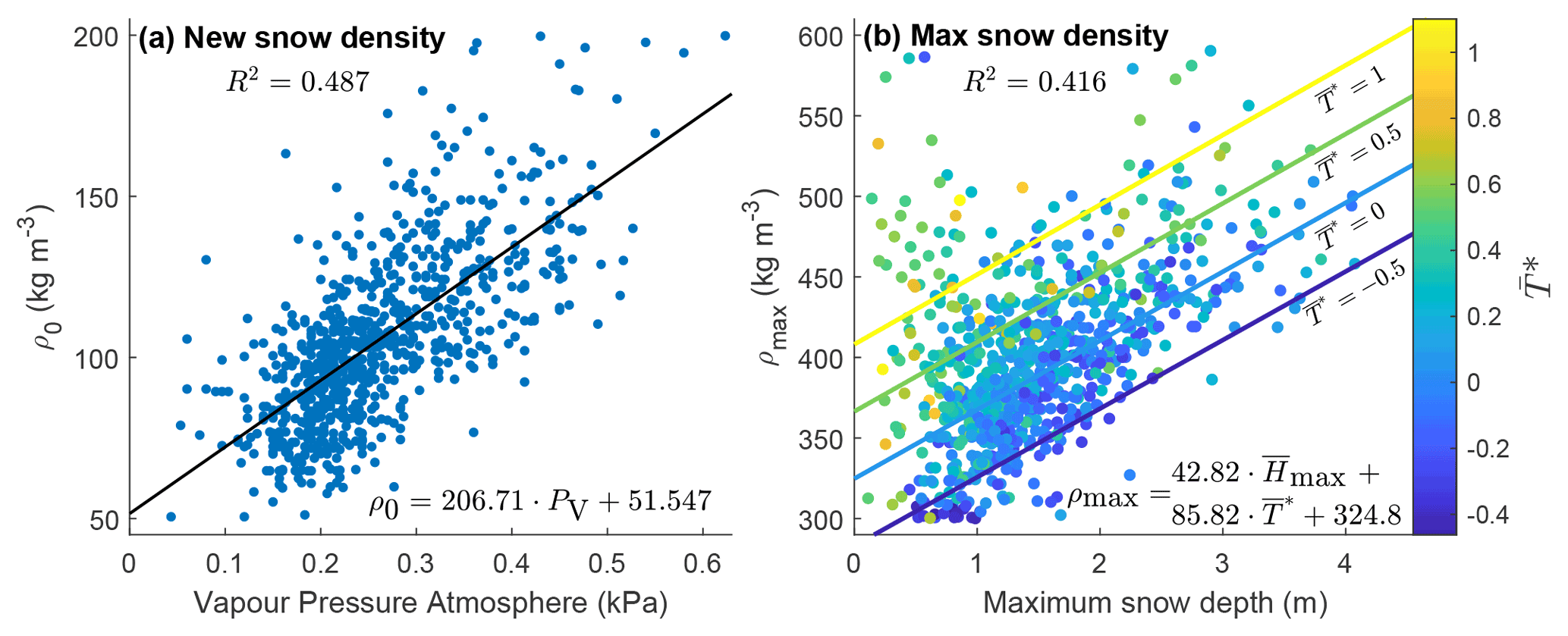
Figure 4Regionalisation of ΔSNOW model parameters. (a) Fresh snow density (ρ0) against mean December–January–February atmospheric vapour pressure (PV) from WorldClim2 dataset. (b) Maximum snow density (ρmax) against maximum snow depth () and dimensionless temperature index (). Equation (2) is shown in panel (a) together with the simple linear regression line. Equation (3) is shown in panel (b) together with regression lines for four values of . Adjusted r-squared is displayed in each panel.
Table 2The ΔSNOW model parameters as originally calibrated by Winkler et al. (2021) and with our regionalised approach (Sect. 3.4).
The new snow density parameter ρ0 is best explained (R2=0.49) by the mean December–January–February (DJF) atmospheric vapour pressure. This influence is consistent with observed climatic controls for snow density, where more humid climates and maritime climates will typically have higher snow densities than drier climates, such as tundra and taiga (Bormann et al., 2013). The maximum snow density parameter ρmax is best explained (R2=0.42) by a combination of the average annual maximum snow depth and . This conforms to broad expectations from snowpack dynamics, whereby the greater mass of a deeper snowpack contributes to higher densification. An estimated value for average annual maximum snow depth should always be available since the model needs continuous time series of snow depth. The dependence on (ratio between mean and amplitude of annual temperature) reveals an additional link between ρmax and the regional climate, whereby close to zero arises for high temperature amplitudes (typically continental climates) or for marginal snow areas with mean annual temperatures close to zero. In contrast, high positive or negative values correspond to low temperature amplitudes (typically maritime climates) or highly negative or positive mean annual temperatures. This relationship can be observed in Fig. 4 if we consider the hypothetical scenario of two sites with equal maximum snow depth. In this case, the site located in a warmer climate is likely to have a higher maximum snow density, which is consistent with previous literature (Bormann et al., 2013).
Based on the two linear regression models, we estimate the new snow density and maximum snow density parameters for all the sites in the regionalisation, evaluation and model input datasets (see Sect. 2) and run the ΔSNOW model for all of the snow depth time series. The performance of the model using these regionalised parameters (ΔSNOWRegionalised) is analysed in Sect. 4.
The final modelled NH-SWE dataset presented in Sect. 5 is based on the parameters estimated using this approach. Furthermore, we provide code for the user to extract the ΔSNOWRegionalised model parameters for any point in the Northern Hemisphere. Latitude–longitude coordinates and a value for maximum snow depth need to be provided by the user (see the “Code and data availability” section).
3.5 Comparison with an alternative SWE estimation approach
In order to provide broader context for our Northern Hemisphere SWE estimates, we compare these results with a previously published statistical SWE estimation model (Hill et al., 2019) (from now on “Hill model”). The Hill model also estimates SWE using snow depth data and climatological variables but does not need a complete time series of snow depth and can instead estimate single values based on an estimate of snow density. There is some similarity in the climatological variables found by Hill et al. (2019) that best estimate snow density variation and those used in the present paper (see Sect. 3.4). The Hill model estimates higher snow density for locations with a higher mean winter precipitation (humid climates) and a lower snow density for locations with a high temperature difference between warmest and coldest month (continental climates). In addition, in the Hill model, the day of the hydrological year contributes to estimating snow density, with higher densities towards the end of the snow season, when the snowpack is deeper and more compact.
We use the WorldClim2 global dataset of monthly climate variables (Fick and Hijmans, 2017) to obtain the Hill model parameters, namely mean winter precipitation (PPTWT) and the temperature difference between the warmest and coldest month (TD). The reader is referred to the work of Hill et al. (2019) for more details on the model. We run the Hill model for all the sites in the regionalisation and evaluation datasets (see Sect. 2). The performance of the Hill model is analysed in Sect. 4 as a comparison along with the regionalised ΔSNOW model (ΔSNOWRegionalised).
3.6 Extended model performance assessment
Previous snow depth to SWE conversion models have evaluated model performance based on root-mean-square error and bias of daily SWE and of peak SWE, which we also employ to enable comparisons. This is mostly due to a lack of data to evaluate more metrics. For example, continuous measurements of SWE are required to assess the model performance on timing of snowmelt onset, but these are rarely available. In order to assist with potential applications in water resources management and modelling, here we use our extensive HS-SWE data compilation (see Sect. 2) to assess additional aspects of the SWE model performance, namely the relative bias of peak SWE, the daily SWE time-series variability, the timing of snowmelt onset, the total snowmelt and the snowmelt duration.
(Nash and Sutcliffe, 1970)Table 3Summary of model performance assessment variables and metrics. All performance variables are computed for each annual snow season. Snow seasons with non-daily SWE observations or with gaps do not allow for the computation of snowmelt onset and snowmelt total. All the biases are computed as modelled minus observed.
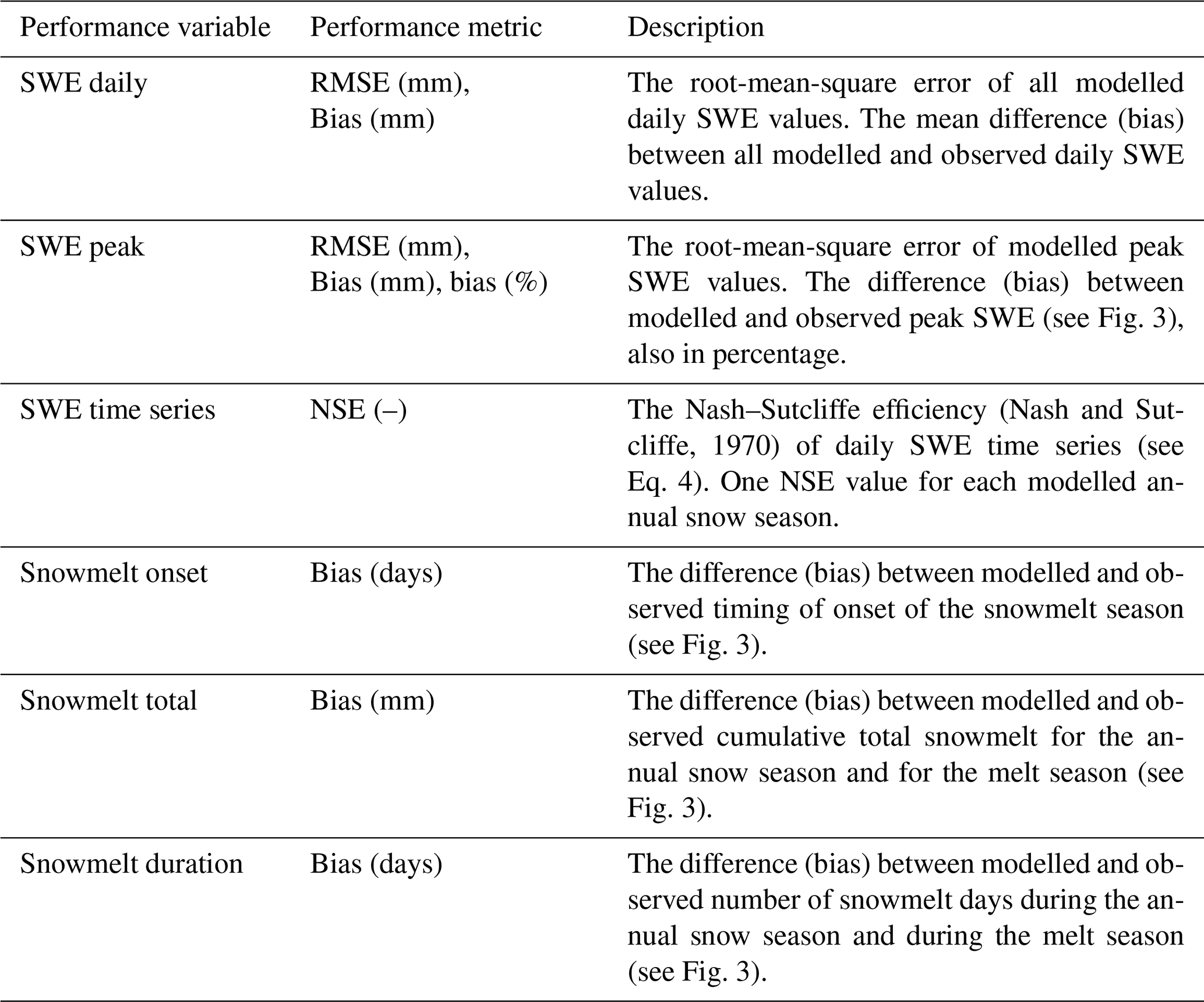
The performance variables and metrics together with their description are shown in Table 3. The reproduction of the daily SWE time series dynamics is assessed based on the well-known Nash–Sutcliffe criterion (Nash and Sutcliffe, 1970), widely used in streamflow model assessment:
where xobs is the observed quantity (here daily SWE) at time step t, xmod is the corresponding modelled quantity and is the mean of all N observed values.
Here we give a summary of the ΔSNOW regionalised (see Sect. 3.6) model performance using both the regionalisation and evaluation datasets.
4.1 Daily SWE, peak SWE and snowmelt onset
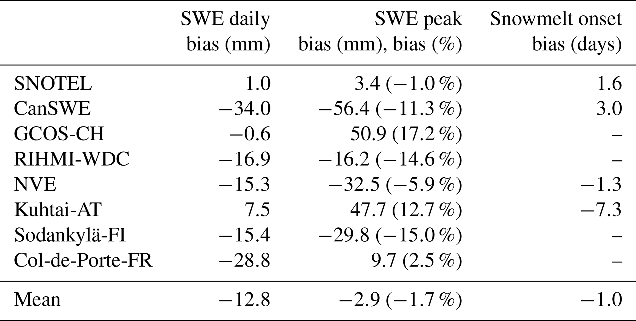
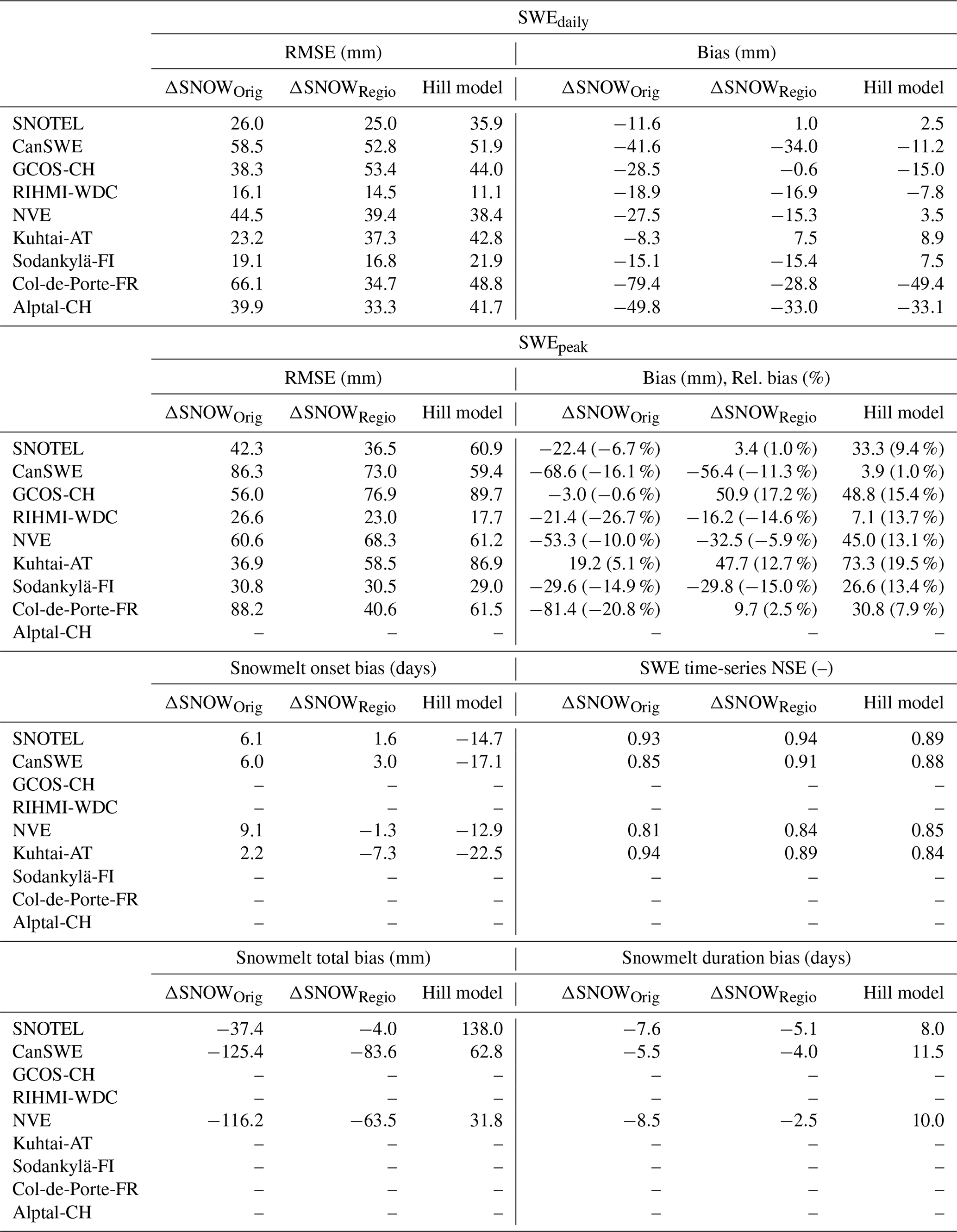
The daily SWE values (Fig. 5a and b) and the peak SWE values (Fig. 5c and d) reproduce the observed values well and show a comparable performance to previous efforts to convert snow depth to snow water equivalent (Jonas et al., 2009; Sturm et al., 2010; Hill et al., 2019; Winkler et al., 2021). The regionalisation dataset is generally unbiased for daily SWE and peak SWE, while the evaluation datasets show a slight but spatially consistent negative bias (Fig. C1). This negative bias is largely driven by the Canadian SWE dataset, because it contains a large amount of data and very deep snowpacks. But the median relative bias across the entire dataset is only −11.3 % (Table 4), and the spatially consistent negative bias is smaller for European sites and for relative bias of peak SWE (Fig. C1). The mean relative bias across all datasets given equal weight is −1.7 %, and the largest relative bias is 17 % (Table 4). For the GCOS-CH and Kuhtai-AT datasets, the regionalisation of parameters yields a lower model performance for daily SWE and peak SWE than using the original ΔSNOW model parameters (see Table C1) obtained for the European Alps. This is because these two datasets were among others used by Winkler et al. (2021) to calibrate the model. It should also be noted that the model from Hill et al. (2019) had a better performance than the ΔSNOW regionalised model for five of the nine datasets used, showing that the Hill model is also an excellent option for estimating daily SWE. The timing of snowmelt onset is well reproduced by the ΔSNOWRegio model, with a 1.45 d bias for the regionalisation dataset and a 1.34 d bias for the evaluation datasets (Fig. 5e and f). The spatial distribution of the bias in snowmelt onset timing shows the dominance of small positive biases except for some sites with a larger positive bias in eastern Canada (Fig. C1). The positive bias in the timing snowmelt onset may indicate a very small model delay in the densification of all the snowpack layers to ρmax. Nonetheless, the model performance is excellent considering no information on daily temperature or any other variable is used to model the start of the snowmelt season. For comparison, the regression model from Hill et al. (2019) has a negative bias of 15 d for the SNOTEL dataset and 17 d for the CanSWE dataset (see Table C1). This very premature onset of the snowmelt season occurs in the regression model because the day of peak SWE corresponds to the day of maximum snow depth, which is not realistic as snowpack compaction and ripening can still occur prior to melt loss. A period of snow depth decline but no change in SWE can last for many days. This can be observed in Fig. 6a. Thus, the improved capacity to capture accurate timing is a key advantage of using the ΔSNOW model.
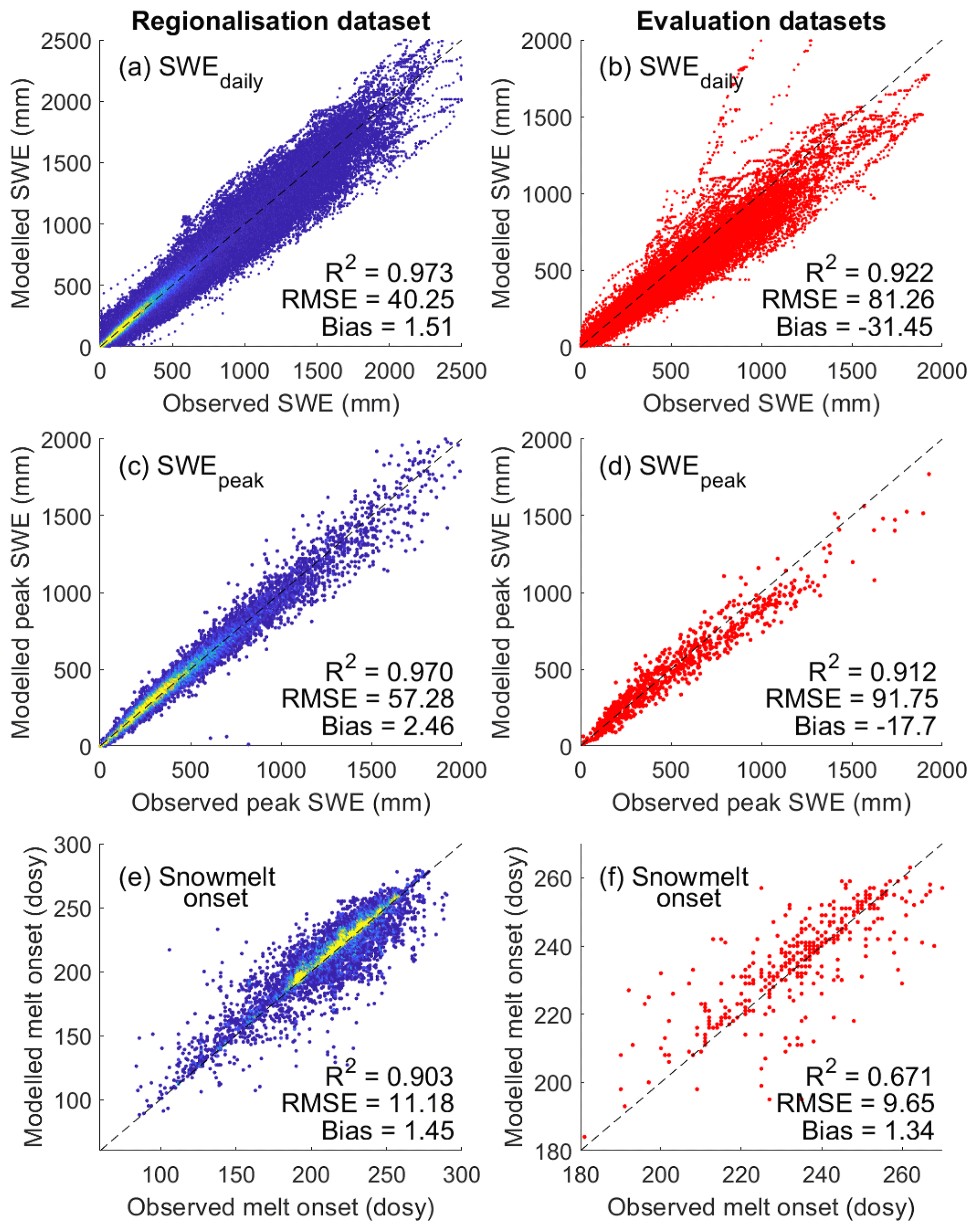
Figure 5Model performance of ΔSNOWRegio. For the regionalisation (a, c, e) and evaluation (b, d, f) datasets, performance of all modelled daily SWE (a, b), modelled peak SWE (c, d) and day of snowmelt onset (e, f) are given. Colours in the left column show scatter density. “dosy”: day of snow year starting on 1 September.
Table 4Performance across datasets for daily SWE, peak SWE and timing of snowmelt onset. For each dataset, the mean performance of all stations is shown. SNOTEL is the regionalisation dataset, and the others are evaluation datasets (see Sect. 2).
4.2 Daily SWE time series
In terms of daily SWE dynamics, Fig. 6b shows that the ΔSNOWRegio model can reach very high Nash–Sutcliffe efficiencies as the bias in daily SWE approaches zero, all data considered. This is shown by the high density of points close to a NSE of 1 in Fig. 6b. In contrast, the regression model from Hill et al. (2019) shows lower NSE values in general for an unbiased daily SWE performance (Fig. 6d), shown by a lower density of points close to a NSE of 1. Only the regionalisation dataset is analysed here, because many time series in the evaluation datasets are not continuous daily measurements and thus do not allow for NSE estimates for the entire snow season. The better performance of the ΔSNOWRegio model is explained by the inclusion of snowpack metamorphism processes which are not included in regression models (e.g. compaction and ripening, see Sect. 3.2). An example can be seen in Fig. 6a and c, where similar unbiased performances for both models show a higher NSE (0.94) for the ΔSNOWRegio compared to the regression model (0.89). The NSE values of modelled daily SWE in Fig. 6a are closer to 1, while the NSE values of the regression model in Fig. 6c are lower and clearly show that the model has difficulty accurately capturing snowpack changes due to daily snow accumulation and settling processes.
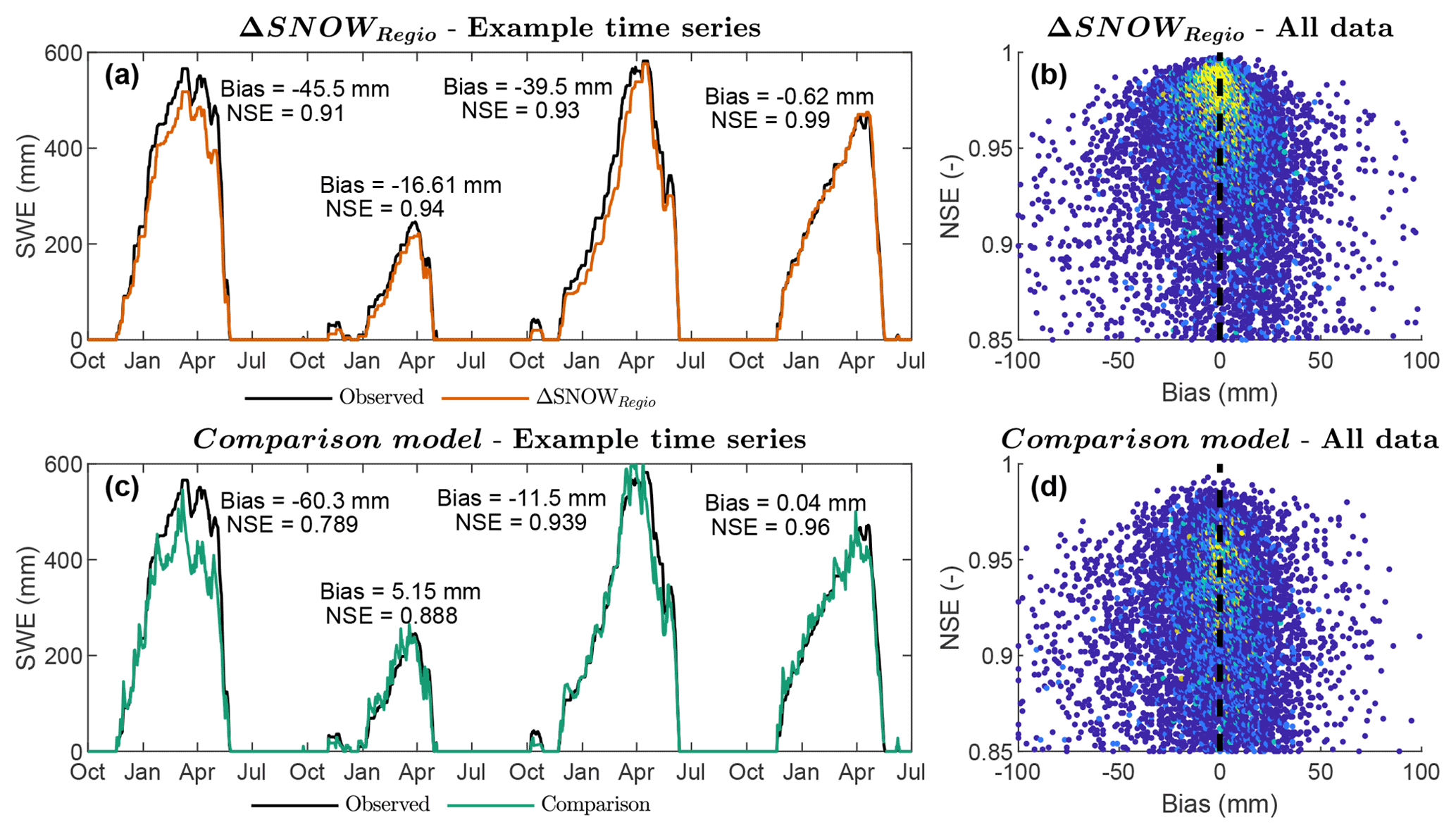
Figure 6Model performance for daily time series. Nash–Sutcliffe efficiency (NSE) vs. bias of daily SWE for (b) the ΔSNOWRegio and (d) the comparison (Hill) model. Colours show scatter point density. One example time series of observed daily SWE and modelled daily SWE for (a) the ΔSNOWRegio and (c) the regression model (Hill model) is shown for comparison. Time series from the 2017–2020 water years of SNOTEL is shown, station ID 371; Buck Flat, Utah, United States; latitude: 39.1300; longitude: −111.44; elevation: 2868 m a.s.l.
4.3 Snowmelt duration and total snowmelt
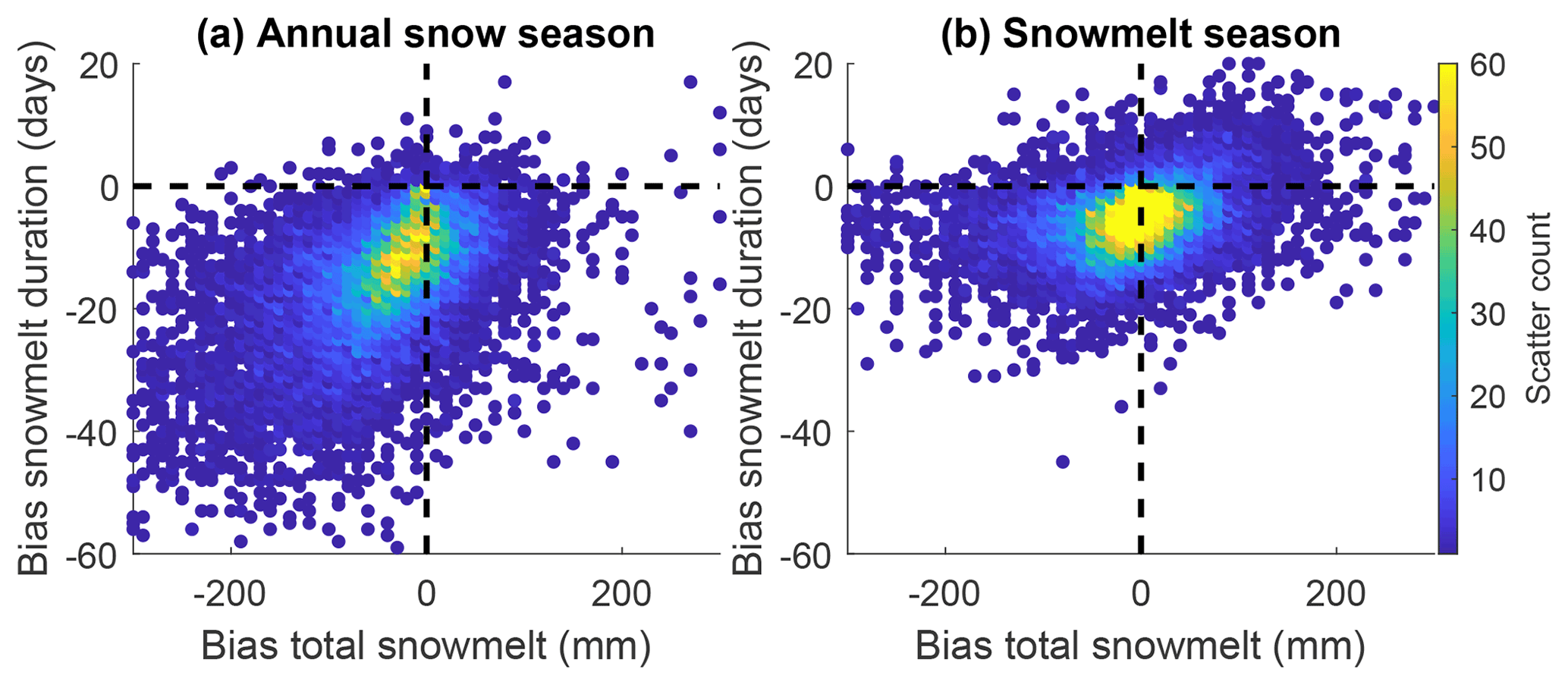
The general daily SWE dynamics are well reproduced by the ΔSNOWRegio model. However, a negative bias in total snowmelt and snowmelt duration is observed when the full annual snow season is considered (Fig. 7a). This negative bias occurs because small snowmelt events (<5 mm) during the accumulation season are not well captured by the ΔSNOWRegio model. The model snow layers do not reach the maximum snow densification for a short period of snowmelt, and the 1 cm precision of snow depth measurements that drive the ΔSNOW model make the minimum modelled melt 3–5 mm (depending on the snow density). During the snowmelt season, the total snowmelt exhibits little to no bias, and the snowmelt duration has a slight negative bias. The negative bias in the duration of the snowmelt season is largely due to the positive bias in the timing of snowmelt onset (2.5 d on average), resulting in a shorter modelled total snowmelt season. Despite the slight negative biases shown for snowmelt duration and total snowmelt, the overall performance is very good and enables confidence in the application of modelled SWE using the ΔSNOWRegio model. This confidence is not possible for regression model estimates of SWE, especially for cumulative variables such as snowmelt duration and total snowmelt, which can be greatly overestimated (although peak SWE magnitudes can be equally well estimated).
4.4 Performance summary
The previous evaluation sections show model performance inclusive of all daily data from the regionalisation and evaluation datasets. In order to provide a more general overview, in Fig. 8 we display a summary comparing three model scenarios, regionalisation and evaluation datasets, and the six different performance metrics (see Table 3). The three model scenarios are the ΔSNOW model with its original parameters from Winkler et al. (2021), the ΔSNOWRegio with our regionalised approach and the Hill model (Hill et al., 2019). Mean performance values for each station are used for forming a boxplot in Fig. 8. This avoids over-weighting performance interpretations due to, for example, stations with very long time series or outliers in model performance. An important highlight from this comparison is the clear benefit in estimating ρ0 and ρ0 from regional climate data (ΔSNOWRegio), which is apparent in the better performance across all six metrics compared to using the original values (ΔSNOWOriginal) obtained by Winkler et al. (2021) for the European Alps only. The full results for all these comparisons are also available in Table C1. The regionalised ΔSNOW model performs better than the original ΔSNOW model for 77 % of all performance metrics and datasets and better than the Hill model for 60 % (see Table C1).
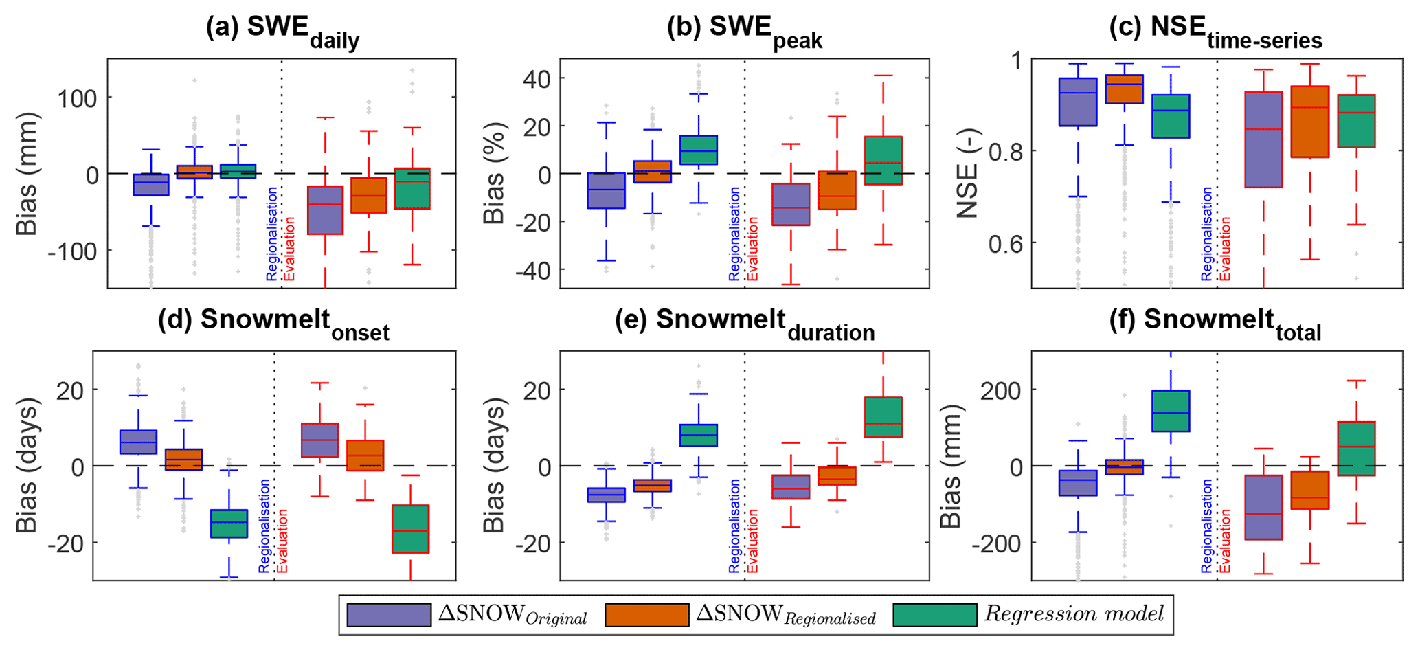
Figure 8Model performance summary. Each subplot is split in two sides: the performance for the regionalisation dataset (left, blue lines) and the performance for the evaluation datasets (right, red lines). Boxes are built from mean values for all stations in each dataset, instead of considering all data points (i.e. a box for the regionalisation dataset is built from the mean performance for that model at each of the 812 SNOTEL sites).
5.1 Snow climatologies and data characteristics
We present an overview of some of the key features of the final NH-SWE dataset in Fig. 9. The dataset contains 11 071 time series of daily SWE and estimated snow density at the point scale. The climatic range is broad, which can be seen in the large variability of peak SWE and of snow cover duration across the sites (Fig. 9a and b). The deepest snowpacks (largest peak SWE) are generally located in high latitudes and mountainous areas, such as western North America, the European Alps and Scandinavia, but deep snowpacks can also occur at high elevation stations surrounded by lower elevation stations with shallow snowpacks, such as the isolated high peak SWE stations that stand out in Poland in Fig. 9a. Snowpacks are generally shallower in relatively warmer locations where higher temperatures limit snowfall (e.g. southern parts of Canada, Germany and Sweden). Shallow snowpacks are also found in very cold climates, where precipitation is limiting due to low water vapour in the atmosphere (e.g. Siberia and northern Canada). Regarding snow cover duration, the spatial patterns are well linked to mean energy availability, with the higher latitudes and higher elevations having the longest snow cover duration.
In Fig. 9c, we compare the links between peak SWE, snow cover duration and . This demonstrates the large variation in the interplay between precipitation and temperature in determining snowpack dynamics. All temperature regimes can produce a low peak-SWE if snow input (i.e. snowfall) is limited. For regimes with low peak-SWE, all snow cover durations are possible, depending on the temperature regime. In very cold climates (e.g. Siberia, Alaska), peak-SWE conditions can last for several months; in warmer climates (e.g. south Scandinavia), the snow will melt quickly.
On the contrary, there is a very clear link between snow cover duration and peak-SWE for temperature regimes that lead to high peak-SWE. In fact, if peak SWE increases, snow cover duration also increase. Peak-SWE convergences to highest values towards intermediate , i.e. neither too cold nor too warm for large amounts of snow to occur and stay for long on the ground.
The median time series length in the dataset is 15 years; however, the distribution is slightly bimodal with the overall average being 35 years, and a second peak in the availability of very long time series (up to 73 years) (Fig. 9d). The distribution of site elevations reflects the large number of time series at low lying parts of coastal Norway, of Canada, and of Siberia. However, more than 1000 sites are located above 1000 m a.s.l., providing good representation of snow dynamics from higher elevations (Fig. 9e).
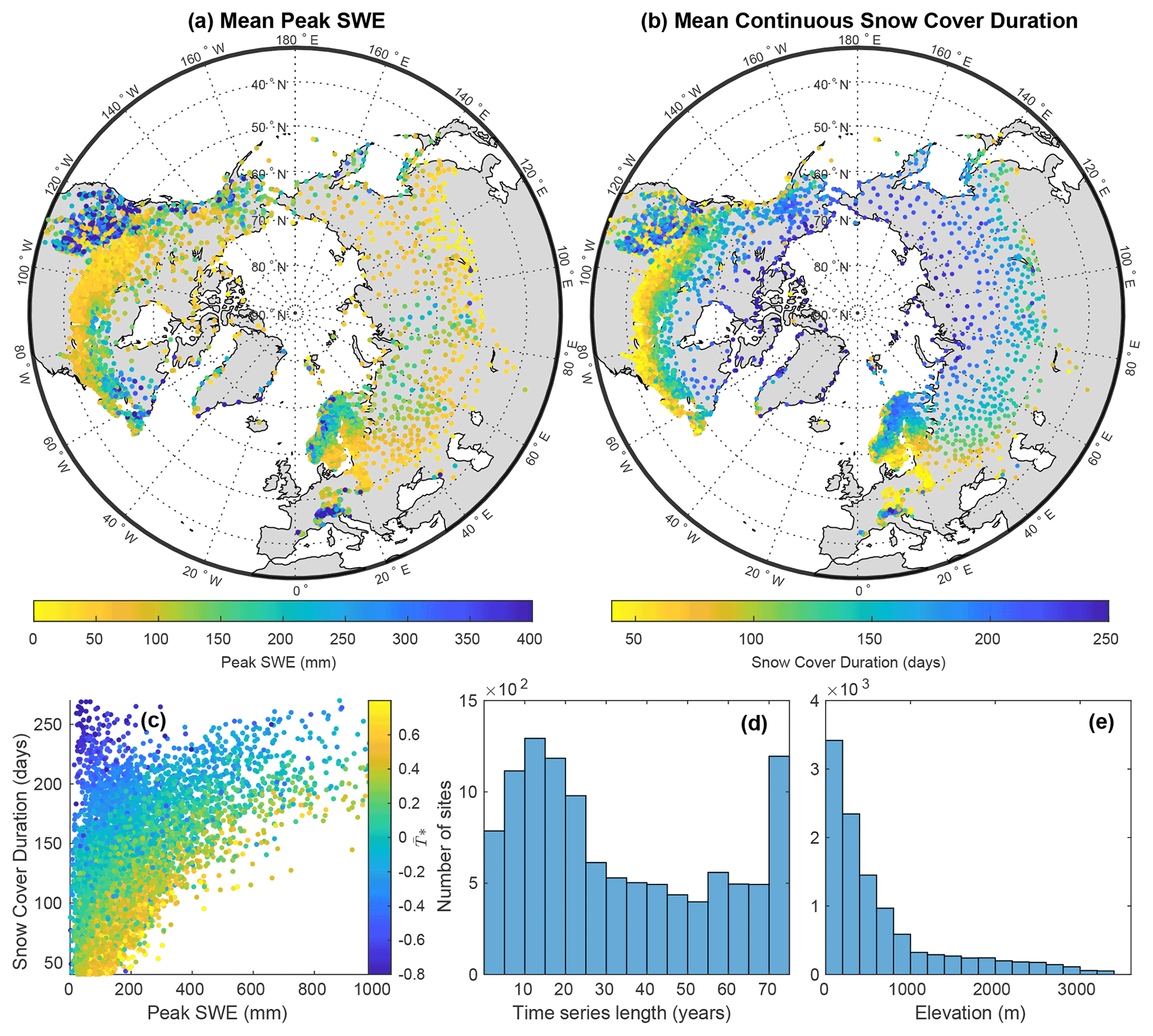
Figure 9Features of the NH-SWE dataset. (a) Mean yearly peak SWE at each station; (b) mean continuous snow cover duration at each station; (c) correlation between peak SWE, snow cover duration and . (d) Distribution of time series lengths in years; and (e) distribution of station elevations.
5.2 Quality control and uncertainty
We provide quality control and uncertainty flags for the SWE time series to signal the values that should be handled with care. We flag the effect of the τ parameter (see Sect. 3.2) on the ΔSNOW model when an increase in snow depth is smaller than τ (2.4 cm). This means that sometimes there is a small increase in snow depth without an increase in SWE, leading to an artificial decrease in snow density. We correct this decrease in snow density and flag the value. Even though this is good for uncertain measurements, care should be taken for snow climates where small snow depth increments are normal. We also flag days when the computed snow density would fall below the fresh snow density parameter value. These are flagged as 1 in the quality control flag in the dataset.
We also flag all the values that result from gap-filling of snow depth. The gap-filling algorithm performs well overall (see Appendix A); however, we cannot guarantee that all gap-filled records are realistic. Special care is required if the data are filled across gaps longer than 15 d because of the reduction in gap-filling performance (see Appendix A). We flag days that are gap-filled with the neural network algorithm with an “N”, and we flag linearly interpolated gaps with an “L”.
6.1 Potential applications
The SWE dataset presented here can be used freely and has a variety of potential applications. This data may be especially useful for applications where an accurate reproduction of the SWE dynamics in terms of timing of snow accumulation and melt is required. Additional uses include data assimilation into hydrological and climate models or validation of remote sensing products. A key strength of the dataset is accuracy in the timing of peak SWE and of snowmelt onset, which makes it valuable for water resources assessment and management. The spatial extent of the dataset offers opportunities for snow climate research and in particular to assess Northern Hemisphere-scale climate change impacts on snow water resources. We note, however, that some key snow regions are not yet included due to lack of long-term data or a lack of data access (e.g. Himalaya, Central Asia and Tibetan Plateau).
The presented NH-SWE dataset is based on a model but also based on actual measurements of snow depth, making this the only point-scale Northern Hemisphere SWE dataset based on in situ snow data. Main advantages compared to other recently published Northern Hemisphere gridded SWE datasets (Luojus et al., 2021; Shao et al., 2022) are the following: (i) NH-SWE includes mountains across the Northern Hemisphere; (ii) it includes deep snowpacks exceeding 200 mm; (iii) it has along temporal coverage, dating back to 1950s for some locations; and (iv) it uses actual point-scale observations of snow depth.
It is noteworthy that we not only publish the NH-SWE dataset but also the underlying ΔSNOW model parameterisation, which can be used to estimate the model parameters for any point in the Northern Hemisphere. In addition, we provide code for this purpose along with the publication of the dataset on Zenodo (see “Code and data availability”), which enables any user to obtain the model parameters to run the ΔSNOW model of Winkler et al. (2021) for any given daily time series of snow depth.
6.2 Limitations
A few limitations should be considered before using the data or our regionalised parameterisation of the ΔSNOW model of Winkler et al. (2021).
Although our analysis applied quality control measures to the daily SNOTEL data used for calibration, potential errors or biases in the data may still exist. As described in the literature, SNOTEL measurements can suffer from overestimation/underestimation of measurement, and these errors are often challenging to detect (Avanzi et al., 2014; Hill et al., 2019). The ΔSNOW model considers the uncertainty associated with snow depth measurements through the threshold deviation parameter (τ=2.4 cm), but larger measurement errors may still be present. Nevertheless, it should be noted that our calibration is based on a sufficiently large sample of data, which likely reduces the impact of potential errors on both the calibration and regionalisation of the model.
Uncertainty in the evaluation datasets should be noted too. Although the evaluation of the SWE estimates for datasets with biweekly measurements (see Table 1) may be somewhat biased due to spatial variability between SWE and HS measurements; the error range for all datasets is similar, indicating that this did not significantly affect the overall model evaluation. The evaluation of the estimated peak SWE provides valid bias measures in terms of SWE magnitude estimates but not in terms of timing, which we do not consider for these biweekly estimates. The peak SWE biases for the datasets with biweekly SWE measurements are also similar to the ones found in the datasets with daily SWE measurements (see Table 1).
The ΔSNOW model requires good quality time series of snow depth (e.g. gap-free, low measurement uncertainty). Measurement errors can accumulate and bias the SWE simulations for an entire season, especially if snow depth data are erroneous for a significant number of days. If the quality of the snow depth observations is poor or not continuous, we recommend using the regression model of Hill et al. (2019) to convert snow depth to SWE.
Our quality control flags capture gap-filled records and unrealistic snow densities, but the amount of data limits our capacity of exhaustive quality checks; unrealistic time series could exist in the dataset. We show that our regional parameterisation performs well especially in terms of snow cover dynamics and timings, but some SWE time series might nevertheless be slightly biased, resulting, for example, from an overestimation or underestimation of model parameters. It is worth noting that while two parameters were calibrated in the regional parameterisation of the ΔSNOW model of Winkler et al. (2021), five other parameters were not calibrated due to data limitations and their lack of clear link with climate variables. However, adding five additional calibration parameters would significantly increase parameter uncertainty, and a thorough sensitivity analysis of the model parameters is provided by Winkler et al. (2021), who highlight the importance of the snow density parameters. Our approach is a prudent one in terms of being able to track assumptions and uncertainty. Despite the lack of calibration of the other parameters, our model evaluation demonstrates that the regionalisation of the density parameters still results in acceptable model performance.
The user should also be cautious with any snow cover duration period of less than 40 d or with snowpacks shallower than 50 mm of SWE. Even though we selected stations with an average of 40 d of snow cover, interannual variability could mean some years are shorter, making the model performance uncertain (see Sect. 2.3). Snow sublimation and snow drift are also processes that are not captured by the ΔSNOW model.
Furthermore, the user should be aware of the spatial and temporal inhomogeneity of NH-SWE; the dataset covers most of the Northern Hemisphere, but some areas have a high station density (e.g. Scandinavia), while others show a rather low density (e.g. Siberia and Alaska). The time series lengths also vary from 1 to 73 years. Finally, NH-SWE does not include the original snow depth data, which has to be directly downloaded from the data source, but we provide modelled snow density along with the SWE time series.
The NH-SWE dataset is free to access and available at https://doi.org/10.5281/zenodo.7515603 (Fontrodona-Bach et al., 2023). The dataset is provided in two different formats (matrices and vectors) and contains modelled daily SWE, estimated snow density, and the quality control and gap-filling flags. An extensive metadata file includes information on station coordinates, elevation, length of time series, model parameters and the climate variables used to estimate them, as well as average snow climatology such as average maximum snow depth, average peak SWE and average maximum snow cover duration. The code used to estimate ΔSNOW regionalised model parameters can be found together with the NH-SWE dataset at https://doi.org/10.5281/zenodo.7515603 (Fontrodona-Bach et al., 2023).
This paper presents NH-SWE, a dataset of snow water equivalent (SWE) time series based on in situ observations of snow depth that are freely available across the Northern Hemisphere. The dataset is based on an established model for continuous snow-depth-to-SWE conversion (Winkler et al., 2021), for which we regionalised the model parameters for application at the Northern Hemisphere scale. The dataset contains 11 071 time series covering most areas of the Northern Hemisphere with a seasonal snow cover and spans the period 1950–2022.
The modelled daily SWE values and seasonal dynamics of SWE are generally well reproduced over the wide range of climates in the regionalisation and evaluation datasets (SNOTEL, CanSWE, GCOS-Switzerland, RIHMI-WDC, NVE and other). The model has a slight delay towards a later start of snowmelt after the peak of snow accumulation, leading to a small negative bias in the duration of the melt season, but peak SWE and total snowmelt are generally unbiased.
Compared to SWE datasets based on remote sensing or climate reanalysis data, with a typical resolution of ∼10 km, NH-SWE is based on in situ observations of snow depth on the ground and therefore provides a higher confidence in the magnitude and dynamics of snow accumulation and melt at the point scale.
This dataset can be used for a variety of applications that require reliable SWE estimates rather than snow depth, in particular in the fields of water resources and snow climate research, environmental and hydrological modelling, validation of remote sensing products, or climate change impact research.
The ΔSNOW model (Winkler et al., 2021) requires a continuous record of daily observations of snow depth to estimate daily SWE. Our compilation of snow depth time series contains a large variability in time series length, number and size of gaps (Fig. A1). Many time series have missing data during the summer period when there is no snow (e.g. most MeteoSwiss stations). This is easy to visually identify and manually fill with zeros, but it is complicated to fill all the series in an automated way with high confidence. Gaps also occur often in the middle of the snow season. Over 90 % of the gaps in the dataset are less than 50 d long, and 80 % of the gaps are less than 10 d long (Fig. A2).
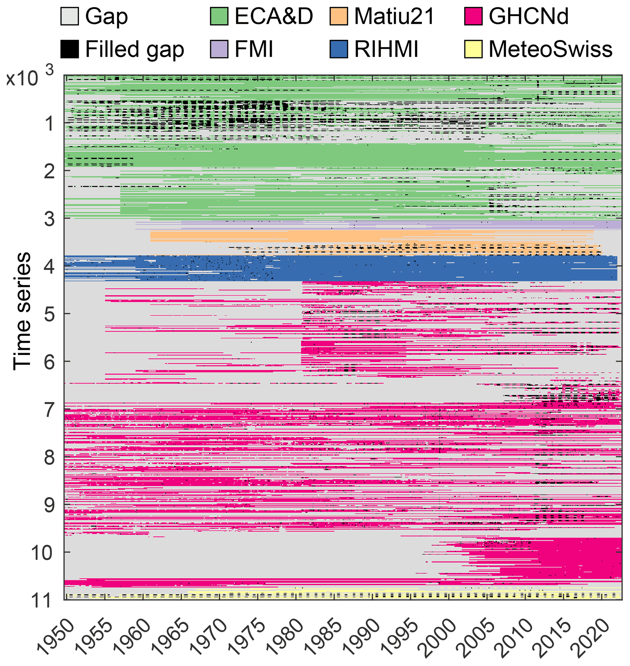
Figure A1Final modelled NH-SWE dataset matrix. Each row corresponds to one of the 11 071 time series in the dataset at daily resolution. Colours indicate data sources, gaps and filled gaps.
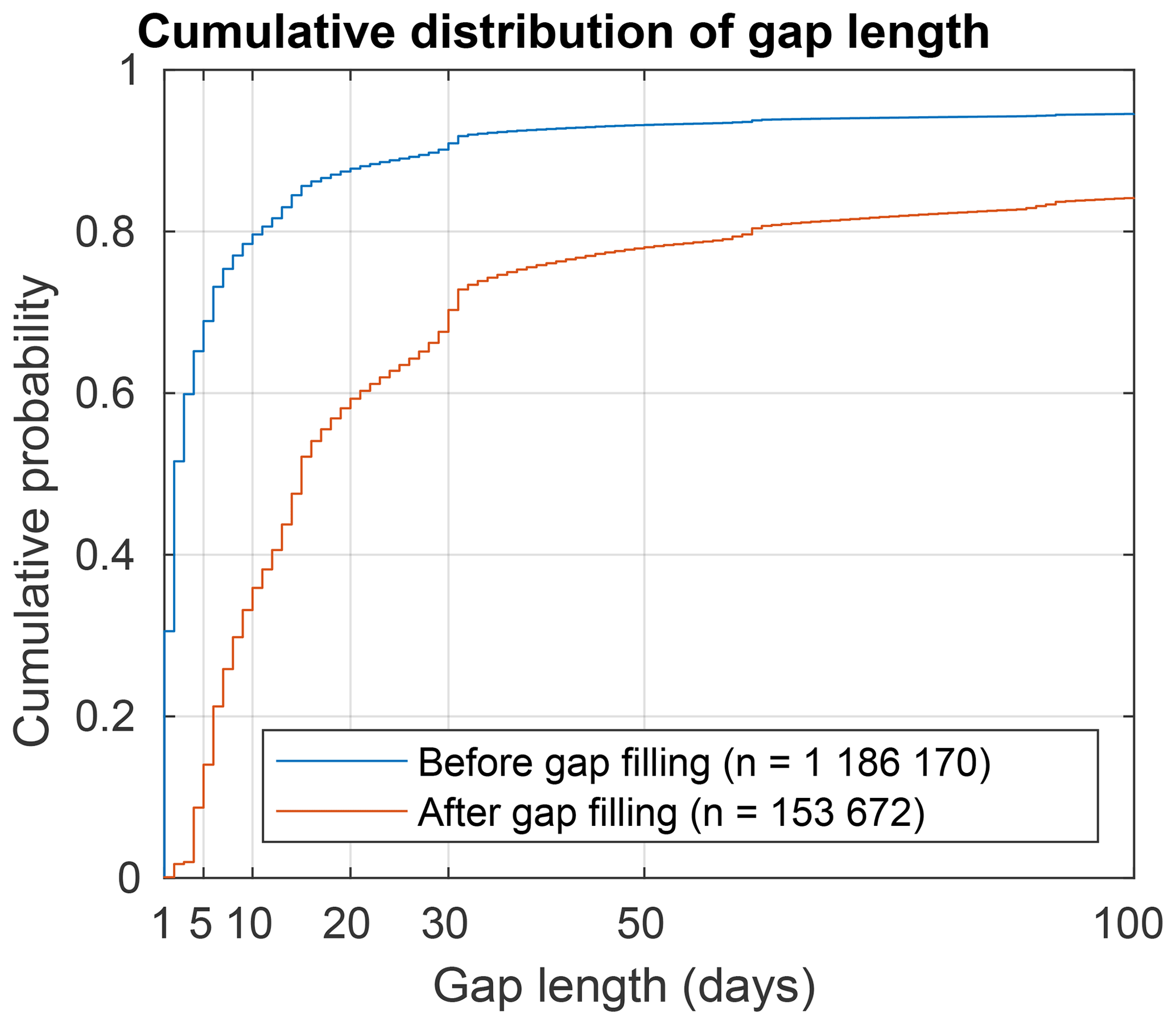
Figure A2Cumulative distribution of dataset gap length before and after gap-filling. n is the total number of data gaps.
The high autocorrelation of daily snow depth time series (i.e. the correlation of snow depth at time t to snow depth at time t−i) motivates us to use a non-linear autoregressive neural network with external input (NARX) technique to fill the time series of snow depth. Neural networks have been used by Silva et al. (2018) and Vieira et al. (2020) to fill environmental time series of sea surface wind speeds and ocean waves but have to date not been applied to snow depth time series. We use the narxnet function from the MATLAB Deep Learning Toolbox (, ). The NARX neural network uses snow depth at time steps up to i d before time t as input to estimate snow depth at time t. The delay parameter i must be estimated. We found i=4 d to be the best estimation of the delay parameter. This means that the snow depth at time t is mostly influenced by snow depth at 1, 2, 3 and 4 d before time t.
External inputs are used to help the NARX simulation. We tested a few NARX network architectures and inputs and found that including precipitation and temperature data as input to the NARX network showed promising results for filling the snow depth time series. We obtain daily precipitation and temperature data from DAYMET (Thornton et al., 2020) for the stations in North America and from E-OBS (Cornes et al., 2018) for the European stations. For the stations in Eurasia not covered by E-OBS, we use temperature and precipitation station data from RIHMI-WDC (2022) stations. For stations where precipitation and temperature data cannot be obtained (i.e. locations not covered by gridded data and no station data available), we do not gap fill the snow depth data with NARX. For stations that were not gap-filled, we only modelled SWE for those years with continuous (gap-free) daily measurements of snow depth.
Neural network models require enough data to be trained. We train one model for each snow depth station in the dataset, because the training of the network could differ per site. During training, the data are divided into a training, a validation and a testing set. The division is made by blocks with a ratio of , meaning that for every 5 years, 3 are used for training, 1 for validation and 1 for testing. For snow depth stations with more than 20 years of data where the trained model yields an r-squared performance higher than 0.9, we further test the performance of the NARX network gap-filling technique by creating synthetic gaps of 1, 3, 7, 15, 30 and 50 d in the time series, at different times of the year. We then run the NARX network gap-filling and compute the absolute error (in centimetres) of the filled snow depth compared to the real observed snow depth. We also compute the percentage error dividing by the observed snow depth value. For each site, we repeat this procedure 50 times so that the gaps are randomly tested at different times of the year, for various years and for various gap lengths. The overall performance of the gap-filling can be visualised in Fig. A3, where the mean absolute error and mean percentage error of the 50 simulations is plotted for each time of the year and gap length. At the beginning of the year (September–October) and at the end (June to August), the mean absolute error is zero, indicating that the NARX neural network performs very well during the summer periods when there is no snow. This allows for filling the gaps in summer with high confidence. During the snow season (November to May), the errors are higher the longer the gap. In percentage terms, the error also becomes larger the longer the gap. We consider an acceptable error to be less than 5 cm or less than 20 %. For gaps equal to or under 15 d, the error of the NARX network gap-filling is consistently under those thresholds. Figure A3 shows the mean over all sites where the performance is tested, but the procedure is applied to each site independently because the training of the network could differ per site.
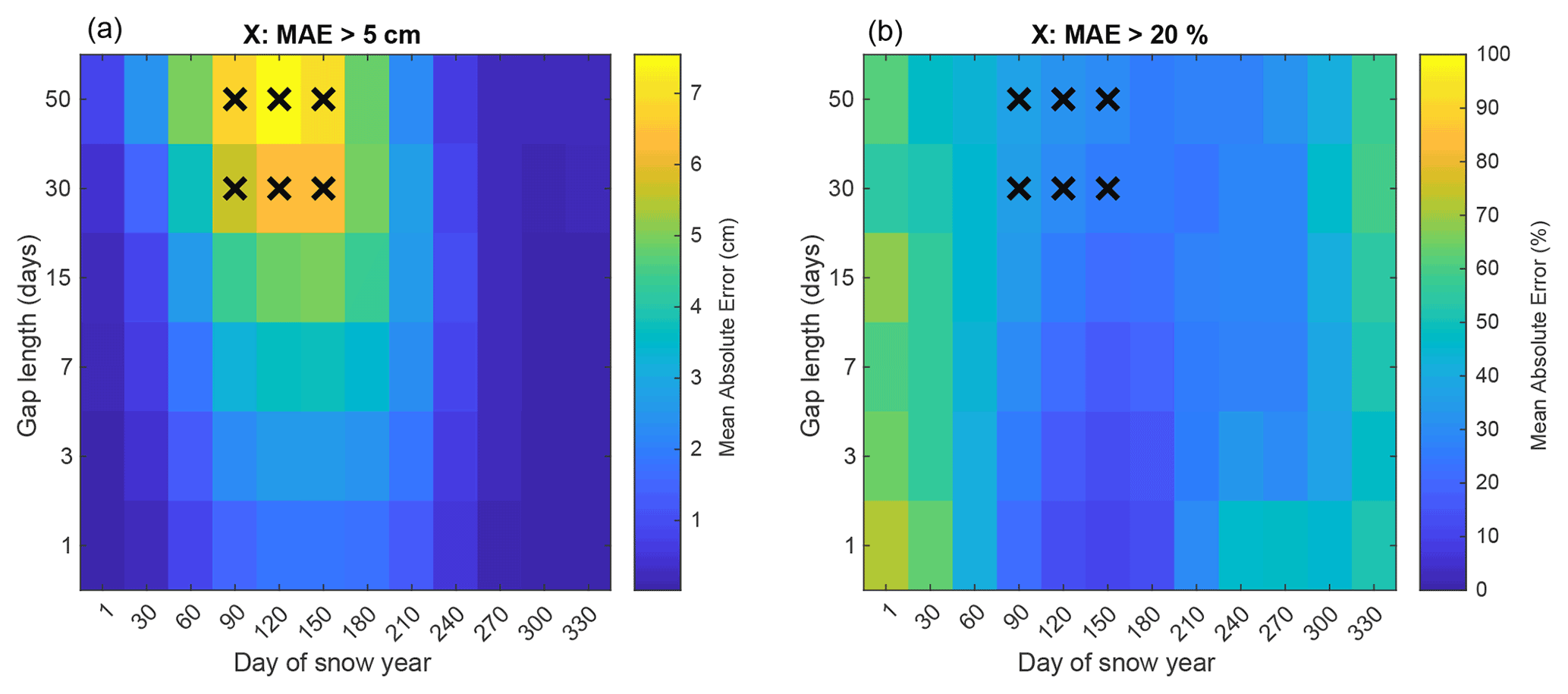
Figure A3Mean performance of NARX gap-filling routine. Panel (a) shows absolute error in centimetres of the snow depth filled gaps at different times of the year and for different gap lengths. Panel (b) shows the same but in percentage error. A cross is displayed if the absolute error is higher than 5 cm and the percentage error is higher than 20 %.
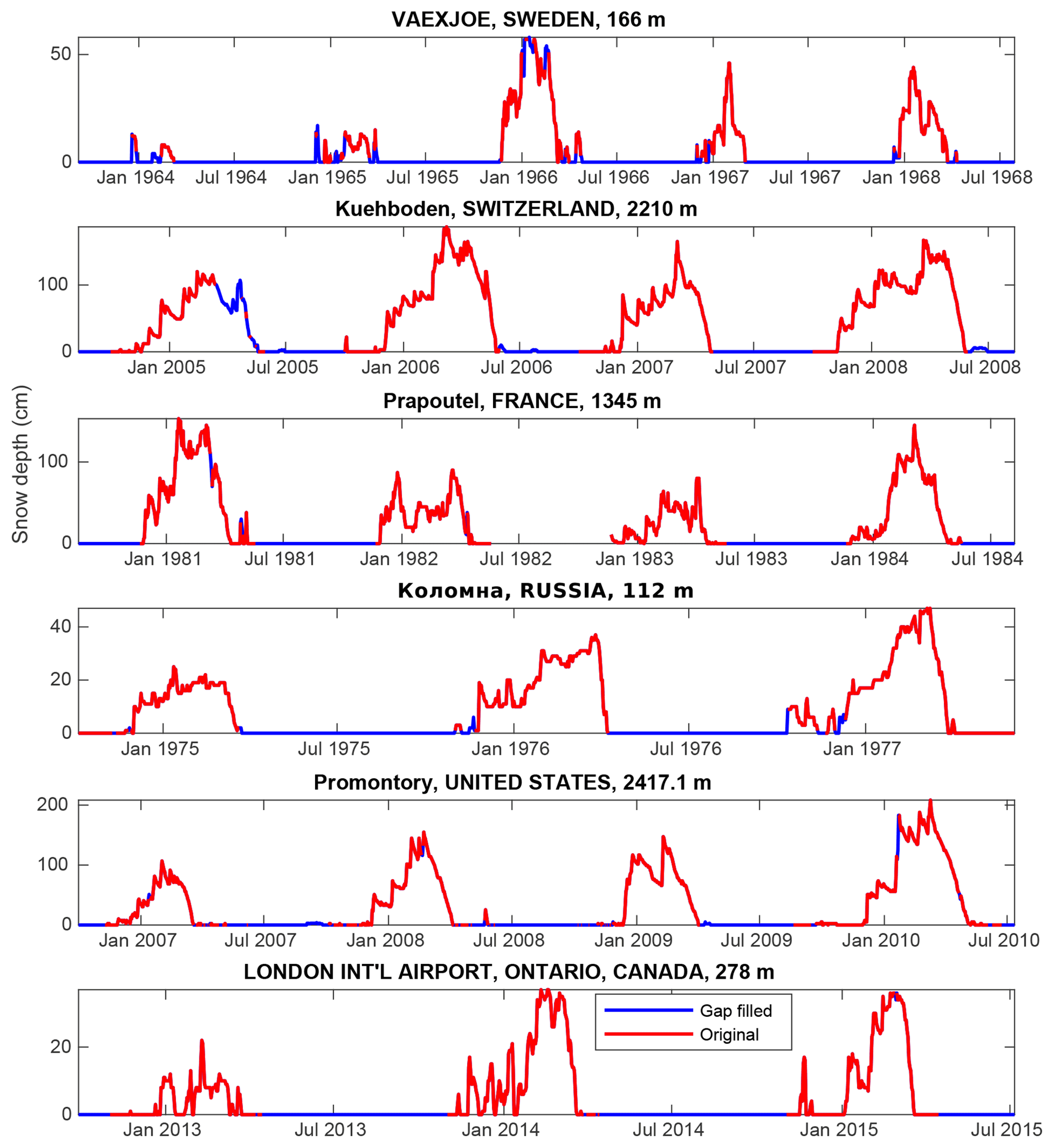
Figure A4Example gap-filled snow depth time series. The title of each subplot corresponds to the station name, the country and the elevation in metres above sea level.
For each gap in each time series, we decide whether or not to fill the gap based on a series of conditions. For stations with a minimum of 20 years of data where the performance is tested as explained above, we fill all the gaps under 16 d long because of the high confidence on filling them (Fig. A3). For gaps longer than 15 d and shorter than 70, we decide based on the performance according to the decision matrix (as in Fig. A3, where an acceptable error is less than 5 cm or less than 20 %) for that specific station. For long gaps between 70 and 365 d, we fill the gaps if the performance for gaps of 50 d is acceptable and at least 80 % of the filled values are under 2 cm of snow depth, which means snow-cover-free periods are being filled. For stations with less than 20 but more than 5 years of data where the training of the NARX model yields an r-squared performance of at least 0.95, we also fill all gaps under 16 d long. For those stations, we also fill longer gaps if at least 80 % of the filled values are under 2 cm, indicating that snow-cover-free summer is being filled. For stations where less than 5 years of daily snow depth data are available but where the NARX model still yields an r-squared performance higher than 0.95, we fill all gaps shorter than 7 d and only fill gaps longer than 7 d if 90 % of the filled values are under 2 cm.
After the NARX neural network gap-filling, we also fill all gaps in the dataset that are equal to or shorter than 3 d by linear interpolation. If a station has more than 20 years of data but the NARX neural network model does not perform well or no precipitation and temperature data are available, we compute the average main snow cover season and we fill with zeros any gaps outside the average snow cover season. If after all the gap-filling routine, 1 snow year at any station has only a gap of 7 d or shorter, we also fill the gap by linear interpolation. We do not fill gaps if any of the conditions above are not met.
Overall, 94.8 % of the filled gaps are filled by the NARX neural network models, while only 5.2 % are linearly interpolated or filled with zeros.
Finally, we apply an extra quality control to the gap-filled time series of snow depth before running the ΔSNOW model. We remove those years where the annual snow season (see Fig. 3) contains more than 75 % of filled gaps. We remove any snow cover period of less than 8 d that is fully gap-filled. We remove those years that are fully snow cover free, given that it is an unlikely event after our selection based on a minimum of 40 d of snow cover on average (see Sect. 2.3). We remove unrealistic daily snow depth increases of more than 150 cm in 1 d or decreases of more than 45 cm in 1 d. These values are based on the 99.99 percentile of all observed daily snow depth increases and snow depth decreases of the entire SNOTEL dataset (see Sect. 2.1). We remove years with perennial snow cover, since the ΔSNOW model is developed over seasonal snowpacks. We remove all snow depth values that are higher than 4 times the median absolute deviation of the average yearly peak of snow depth.
Figure A4 shows example time series where the gap-filling is successfully filling the summer zeroes and small gaps during the snow season.
We test a few climate variables to regionalise the ΔSNOW model parameters in Sect. 3.4. All the climate variables are obtained from the WorldClim2 dataset of monthly climate variables (Fick and Hijmans, 2017). We complete the set of climate variables with snow climatology variables (i.e. climate variables based on snow depth data). The variables that were computed and tested are the following:
-
: mean yearly temperature
-
: mean December–January–February temperature
-
: mean November–December–January–February–March temperature
-
: mean December–January–February cumulative precipitation
-
: mean November–December–January–February–March cumulative precipitation
-
: precipitation as snow computed as the sum of monthly precipitation when temperature is below zero
-
: dimensionless temperature index from Woods (2009) defined as the ratio between mean annual temperature and the amplitude of the annual temperature cycle
-
: dimensionless precipitation index from Woods (2009) comparing the average precipitation rate and melt rate for a site
-
PV,DJF: mean December–January–February vapour pressure in the atmosphere
-
PV,NDJFM: mean December–January–February vapour pressure in the atmosphere
-
SR,DJF: mean December–January–February short-wave radiation
-
PR,NDJFM: mean December–January–February short-wave radiation
-
: mean snow depth
-
: mean maximum snow depth (i.e. peak of snow accumulation)
This extends the model performance summary of Sect. 4, showing the mean model performance for each of the datasets separately for three model scenarios (ΔSNOW original, ΔSNOW regionalised and Hill model) and for the six evaluation metrics from Table 3.
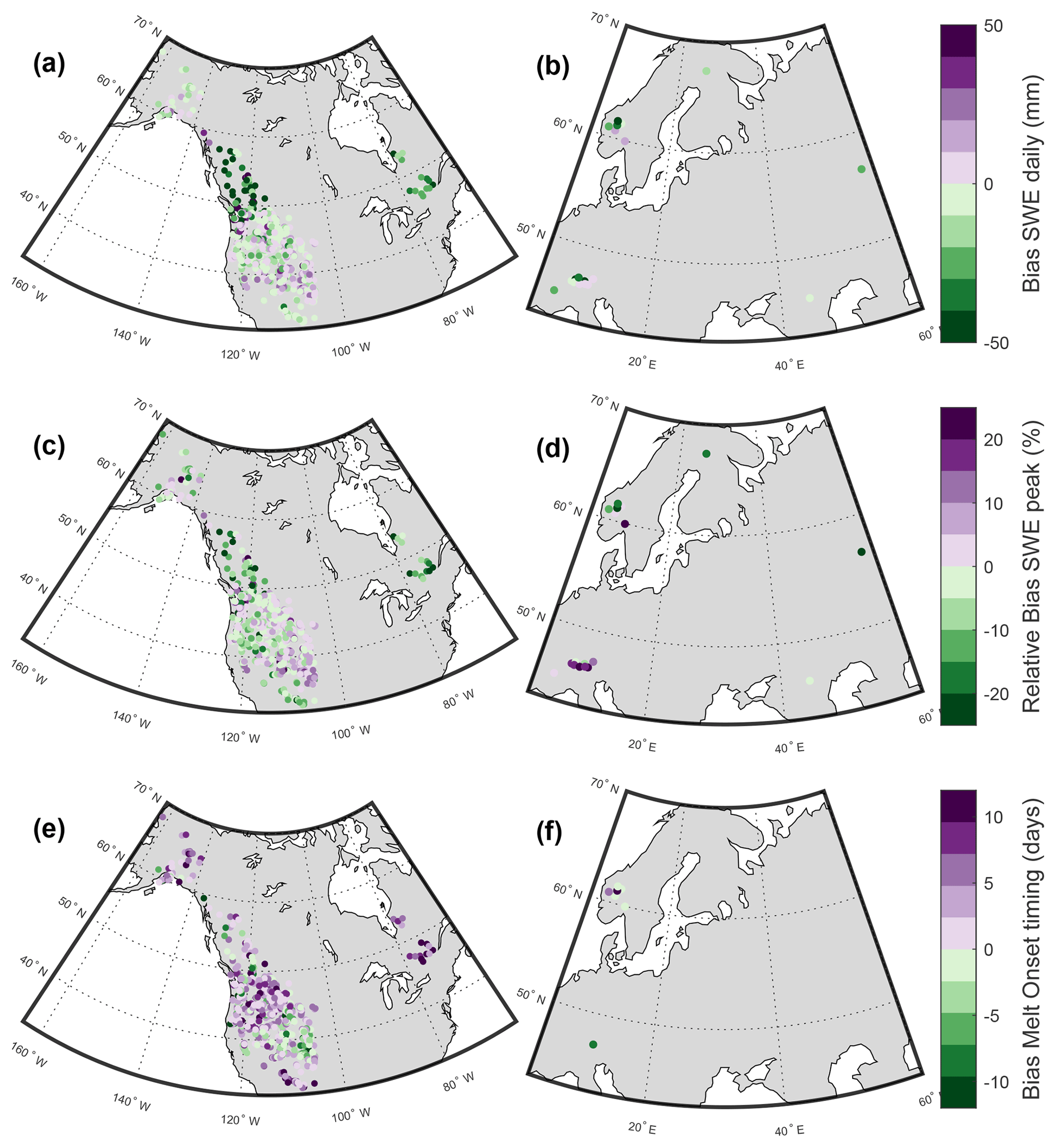
Figure C1Spatial distribution of model performance. The variables shown are the same as in Table 4: Panels (a) and (b) for bias of daily SWE, panels (c) and (d) for relative bias of peak SWE, and panels (e) and (f) for bias of snowmelt onset timing. All sites displayed are from regionalisation and evaluation datasets.
Table C1Extended model performance and evaluation. Here the performances are shown for all the datasets separately. ΔSNOWOrig refers to the original model parameters by Winkler et al. (2021), ΔSNOWRegio refers to our regional parameterisation (see Sect. 3.4) and Hill model refers to the regression model from Winkler et al. (2021). Where a value is not shown, it means that performance variable is not possible to compute for that dataset due to a lack of appropriate observed SWE records to compute that metric. The ΔSNOWRegio is better than ΔSNOWOrig on 77 % of all datasets and metrics and better than the Hill model on 61 % of all datasets and metrics.
AFB collected and processed the data, calibrated and parameterised the model, wrote the manuscript, produced all the figures and results, and provided the SWE dataset. JRL closely supervised the underlying PhD research and wrote the initial PhD project proposal. JRL and BS contributed to editing the text. AJT had the initial idea of producing a SWE dataset based on depth data. BS, RW and AJT gave regular input on the work and the manuscript process. All co-authors have provided feedback on the manuscript.
The contact author has declared that none of the authors has any competing interests.
Publisher's note: Copernicus Publications remains neutral with regard to jurisdictional claims in published maps and institutional affiliations.
Adrià Fontrodona-Bach acknowledges the UK's Natural Environment Research Council (NERC) CENTA2 doctoral training programme. The computations described in this paper were performed using the University of Birmingham's BlueBEAR HPC service, which provides a high performance computing service to the University's research community. See http://www.birmingham.ac.uk/bear (last access: 20 January 2023) for more details.
This research has been supported by the Natural Environment Research Council (CENTA studentship).
This paper was edited by Dalei Hao and reviewed by Ning Sun and one anonymous referee.
Avanzi, F., De Michele, C., Ghezzi, A., Jommi, C., and Pepe, M.: A processing–modeling routine to use SNOTEL hourly data in snowpack dynamic models, Adv. Water Resour., 73, 16–29, 2014. a
Beniston, M., Farinotti, D., Stoffel, M., Andreassen, L. M., Coppola, E., Eckert, N., Fantini, A., Giacona, F., Hauck, C., Huss, M., Huwald, H., Lehning, M., López-Moreno, J.-I., Magnusson, J., Marty, C., Morán-Tejéda, E., Morin, S., Naaim, M., Provenzale, A., Rabatel, A., Six, D., Stötter, J., Strasser, U., Terzago, S., and Vincent, C.: The European mountain cryosphere: a review of its current state, trends, and future challenges, The Cryosphere, 12, 759–794, https://doi.org/10.5194/tc-12-759-2018, 2018. a
Bormann, K. J., Westra, S., Evans, J. P., and McCabe, M. F.: Spatial and temporal variability in seasonal snow density, J. Hydrol., 484, 63–73, 2013. a, b, c
Bormann, K. J., Brown, R. D., Derksen, C., and Painter, T. H.: Estimating snow-cover trends from space, Nat. Clim. Change, 8, 924–928, 2018. a
Broxton, P. D., Zeng, X., and Dawson, N.: Why do global reanalyses and land data assimilation products underestimate snow water equivalent?, J. Hydrometeorol., 17, 2743–2761, 2016. a
Brun, E., Vionnet, V., Boone, A., Decharme, B., Peings, Y., Valette, R., Karbou, F., and Morin, S.: Simulation of northern Eurasian local snow depth, mass, and density using a detailed snowpack model and meteorological reanalyses, J. Hydrometeorol., 14, 203–219, 2013. a
Clark, M. P., Hendrikx, J., Slater, A. G., Kavetski, D., Anderson, B., Cullen, N. J., Kerr, T., Örn Hreinsson, E., and Woods, R. A.: Representing spatial variability of snow water equivalent in hydrologic and land-surface models: A review, Water Resour. Res., 47, W07539, https://doi.org/10.1029/2011WR010745, 2011. a
Cornes, R. C., van der Schrier, G., van den Besselaar, E. J., and Jones, P. D.: An ensemble version of the E-OBS temperature and precipitation data sets, J. Geophys. Res.-Atmos., 123, 9391–9409, 2018. a
Dawson, N., Broxton, P., and Zeng, X.: A New Snow Density Parameterization for Land Data Initialization, J. Hydrometeorol., 18, 197–207, https://doi.org/10.1175/JHM-D-16-0166.1, 2017. a
Déry, S. J. and Brown, R. D.: Recent Northern Hemisphere snow cover extent trends and implications for the snow-albedo feedback, Geophys. Res. Lett., 34, L22504, https://doi.org/10.1029/2007GL031474, 2007. a
Essery, R., Kontu, A., Lemmetyinen, J., Dumont, M., and Ménard, C. B.: A 7-year dataset for driving and evaluating snow models at an Arctic site (Sodankylä, Finland), Geosci. Instrum. Method. Data Syst., 5, 219–227, https://doi.org/10.5194/gi-5-219-2016, 2016. a, b
Fick, S. E. and Hijmans, R. J.: WorldClim 2: new 1-km spatial resolution climate surfaces for global land areas, Int. J. Climatol., 37, 4302–4315, 2017. a, b, c, d, e
FMI: Open Research Data from the Finnish Meteorological Institute, Finnish Meteorological Institute [data set], https://en.ilmatieteenlaitos.fi/observation-stations (last access: 22 September 2022), 2022. a
Fontrodona Bach, A., Van der Schrier, G., Melsen, L., Klein Tank, A., and Teuling, A.: Widespread and accelerated decrease of observed mean and extreme snow depth over Europe, Geophys. Res. Lett., 45, 12–312, 2018. a, b, c
Fontrodona-Bach, A., Schaefli, B., Woods, R., Teuling, A. J., and Larsen, J.: NH-SWE: Northern Hemisphere Snow Water Equivalent dataset based on in-situ snow depth time series and the regionalisation of the ΔSNOW model, Zenodo [data set], https://doi.org/10.5281/zenodo.7515603, 2023. a, b, c
Hill, D. F., Burakowski, E. A., Crumley, R. L., Keon, J., Hu, J. M., Arendt, A. A., Wikstrom Jones, K., and Wolken, G. J.: Converting snow depth to snow water equivalent using climatological variables, The Cryosphere, 13, 1767–1784, https://doi.org/10.5194/tc-13-1767-2019, 2019. a, b, c, d, e, f, g, h, i, j, k, l, m, n, o
Jonas, T., Marty, C., and Magnusson, J.: Estimating the snow water equivalent from snow depth measurements in the Swiss Alps, J. Hydrol., 378, 161–167, 2009. a, b, c, d, e
Klein Tank, A. M. G., Wijngaard, J. B., Können, G.P ., Böhm, R., Demarée, G., Gocheva, A., Mileta, M., Pashiardis, S., Hejkrlik, L., Kern-Hansen, C., Heino, R., Bessemoulin, P., Müller-Westermeier, G., Tzanakou, M., Szalai, S., Pálsdóttir, T., Fitzgerald, D., Rubin, S., Capaldo, M., Maugeri, M., Leitass, A., Bukantis, A., Aberfeld, R., van Engelen, A. F. V., Forland, E., Mietus, M., Coelho, F., Mares, C., Razuvaev, V., Nieplova, E., Cegnar, T., Antonio López, J., Dahlström, B., Moberg, A., Kirchhofer, W., Ceylan, A., Pachaliuk, O., Alexander, L. V., and Petrovic, P.: Daily dataset of 20th-century surface air temperature and precipitation series for the European Climate Assessment, Int. J. Climatol., 22, 1441–1453, 2002. a, b
Krajči, P., Kirnbauer, R., Parajka, J., Schöber, J., and Blöschl, G.: The Kühtai data set: 25 years of lysimetric, snow pillow, and meteorological measurements, Water Resour. Res., 53, 5158–5165, 2017. a, b
Kuppel, S., Fan, Y., and Jobbágy, E. G.: Seasonal hydrologic buffer on continents: Patterns, drivers and ecological benefits, Adv. Water Resour., 102, 178–187, 2017. a
López-Moreno, J., Soubeyroux, J. M., Gascoin, S., Alonso-Gonzalez, E., Durán-Gómez, N., Lafaysse, M., Vernay, M., Carmagnola, C., and Morin, S.: Long-term trends (1958–2017) in snow cover duration and depth in the Pyrenees, Int. J. Climatol., 40, 6122–6136, 2020. a
López-Moreno, J. I., Fassnacht, S., Heath, J., Musselman, K., Revuelto, J., Latron, J., Morán-Tejeda, E., and Jonas, T.: Small scale spatial variability of snow density and depth over complex alpine terrain: Implications for estimating snow water equivalent, Adv. Water Resour., 55, 40–52, 2013. a
Luojus, K., Pulliainen, J., Takala, M., Lemmetyinen, J., Mortimer, C., Derksen, C., Mudryk, L., Moisander, M., Hiltunen, M., Smolander, T., Ikonen, J., Cohen, J., Salminen, M., Norberg, J., Veijola, K., and Venäläinen, P.: GlobSnow v3. 0 Northern Hemisphere snow water equivalent dataset, Sci. Data, 8, 1–16, 2021. a, b
Mankin, J. S., Viviroli, D., Singh, D., Hoekstra, A. Y., and Diffenbaugh, N. S.: The potential for snow to supply human water demand in the present and future, Environ. Res. Lett., 10, 114016, https://doi.org/10.1088/1748-9326/10/11/114016, 2015. a
Marty, C.: GCOS SWE data from 11 stations in Switzerland, WSL Institute for Snow and Avalanche Research SLF [data set], https://doi.org/10.16904/15 (last access: 30 October 2020), 2020. a, b
Matiu, M., Crespi, A., Bertoldi, G., Carmagnola, C. M., Marty, C., Morin, S., Schöner, W., Cat Berro, D., Chiogna, G., De Gregorio, L., Kotlarski, S., Majone, B., Resch, G., Terzago, S., Valt, M., Beozzo, W., Cianfarra, P., Gouttevin, I., Marcolini, G., Notarnicola, C., Petitta, M., Scherrer, S. C., Strasser, U., Winkler, M., Zebisch, M., Cicogna, A., Cremonini, R., Debernardi, A., Faletto, M., Gaddo, M., Giovannini, L., Mercalli, L., Soubeyroux, J.-M., Sušnik, A., Trenti, A., Urbani, S., and Weilguni, V.: Observed snow depth trends in the European Alps: 1971 to 2019, The Cryosphere, 15, 1343–1382, https://doi.org/10.5194/tc-15-1343-2021, 2021a. a, b, c, d
Matiu, M., Crespi, A., Bertoldi, G., Carmagnola, C. M., Marty, C., Morin, S., Schöner, W., Cat Berro, D., Chiogna, G., De Gregorio, L., Kotlarski, S., Majone, B., Resch, G., Terzago, S., Valt, M., Beozzo, W., Cianfarra, P., Gouttevin, I., Marcolini, G., Notarnicola, C., Petitta, M., Scherrer, S. C., Strasser, U., Winkler, M., Zebisch, M., Cicogna, A., Cremonini, R., Debernardi, A., Faletto, M., Gaddo, M., Giovannini, L., Mercalli, L., Soubeyroux, J.-M., Sušnik, A., Trenti, A., Urbani, S., and Weilguni, V.: Snow cover in the European Alps: Station observations of snow depth and depth of snowfall, Zenodo [data set], https://doi.org/10.5281/zenodo.5109574, 2021b. a, b
MATLAB R2021a: MATLAB Deep Learning Toolbox, https://www.mathworks.com/products/deep-learning (last access: 20 January 2023), the MathWorks, Natick, MA, USA, R2021a. a
McCreight, J. L. and Small, E. E.: Modeling bulk density and snow water equivalent using daily snow depth observations, The Cryosphere, 8, 521–536, https://doi.org/10.5194/tc-8-521-2014, 2014. a, b
McKay, M. D., Beckman, R. J., and Conover, W. J.: A Comparison of Three Methods for Selecting Values of Input Variables in the Analysis of Output from a Computer Code, Technometrics, 21, 239–245, 1979. a
Menne, M. J., Durre, I., Vose, R. S., Gleason, B. E., and Houston, T. G.: An overview of the global historical climatology network-daily database, J. Atmos. Ocean. Tech., 29, 897–910, 2012. a
MeteoSwiss: Open Research Data from the Swiss Meteorological Service through the IDAWEB portal. Includes station data from Meteoswiss, the SLF (WSL Institute for Snow and Avalance Research), and the Autonomous Province of Bolzano – Sudtirol, MeteoSwiss [data set], https://gate.meteoswiss.ch/idaweb/ (last access: 27 September 2023), 2022. a
Mizukami, N. and Perica, S.: Spatiotemporal characteristics of snowpack density in the mountainous regions of the western United States, J. Hydrometeorol., 9, 1416–1426, 2008. a
Morin, S., Lejeune, Y., Lesaffre, B., Panel, J.-M., Poncet, D., David, P., and Sudul, M.: An 18-yr long (1993–2011) snow and meteorological dataset from a mid-altitude mountain site (Col de Porte, France, 1325 m alt.) for driving and evaluating snowpack models, Earth Syst. Sci. Data, 4, 13–21, https://doi.org/10.5194/essd-4-13-2012, 2012. a, b
Mudryk, L., Derksen, C., Kushner, P., and Brown, R.: Characterization of Northern Hemisphere snow water equivalent datasets, 1981–2010, J. Climate, 28, 8037–8051, 2015. a
Mudryk, L., Santolaria-Otín, M., Krinner, G., Ménégoz, M., Derksen, C., Brutel-Vuilmet, C., Brady, M., and Essery, R.: Historical Northern Hemisphere snow cover trends and projected changes in the CMIP6 multi-model ensemble, The Cryosphere, 14, 2495–2514, https://doi.org/10.5194/tc-14-2495-2020, 2020. a
Muñoz-Sabater, J., Dutra, E., Agustí-Panareda, A., Albergel, C., Arduini, G., Balsamo, G., Boussetta, S., Choulga, M., Harrigan, S., Hersbach, H., Martens, B., Miralles, D. G., Piles, M., Rodríguez-Fernández, N. J., Zsoter, E., Buontempo, C., and Thépaut, J.-N.: ERA5-Land: a state-of-the-art global reanalysis dataset for land applications, Earth Syst. Sci. Data, 13, 4349–4383, https://doi.org/10.5194/essd-13-4349-2021, 2021. a
Musselman, K. N., Addor, N., Vano, J. A., and Molotch, N. P.: Winter melt trends portend widespread declines in snow water resources, Nat. Clim. Change, 11, 418–424, 2021. a
Nash, J. E. and Sutcliffe, J. V.: River flow forecasting through conceptual models. Part I, a discussion of principles, J. Hydrol., 10, 282–290, 1970. a, b
Notarnicola, C.: Hotspots of snow cover changes in global mountain regions over 2000–2018, Remote Sens. Environ., 243, 111781, https://doi.org/10.1016/j.rse.2020.111781, 2020. a
Ntokas, K. F. F., Odry, J., Boucher, M.-A., and Garnaud, C.: Investigating ANN architectures and training to estimate snow water equivalent from snow depth, Hydrol. Earth Syst. Sci., 25, 3017–3040, https://doi.org/10.5194/hess-25-3017-2021, 2021. a
NVE: Open Research Data from Norwegian Water Resources and Energy Directorate [dataset], Norwegian Water Resources and Energy Directorate, https://www.nve.no/hydrologi/sno/automatiske-snostasjoner/?ref=mainmenu (last access: 23 March 2021), 2022. a, b
Pistocchi, A.: Simple estimation of snow density in an Alpine region, J. Hydrol.-Regional Studies, 6, 82–89, 2016. a
RIHMI-WDC: Open Research Data from the All-Russia Research Institute of Hydrometeorological Information – World Data Center, All-Russia Research Institute of Hydrometeorological Information [data set], http://meteo.ru/data/165-snow-cover (last access: 22 September 2022), 2022. a, b, c, d
Serreze, M. C., Clark, M. P., Armstrong, R. L., McGinnis, D. A., and Pulwarty, R. S.: Characteristics of the western United States snowpack from snowpack telemetry (SNOTEL) data, Water Resour. Res., 35, 2145–2160, 1999. a
Shao, D., Li, H., Wang, J., Hao, X., Che, T., and Ji, W.: Reconstruction of a daily gridded snow water equivalent product for the land region above 45° N based on a ridge regression machine learning approach, Earth Syst. Sci. Data, 14, 795–809, https://doi.org/10.5194/essd-14-795-2022, 2022. a
Silva, M. T., Gill, E. W., and Huang, W.: An improved estimation and gap-filling technique for sea surface wind speeds using NARX neural networks, J. Atmos. Ocean. Tech., 35, 1521–1532, 2018. a
Stähli, M.: Longterm hydrological observatory Alptal (central Switzerland), https://www.envidat.ch/dataset/longterm-hydrological-observatory-alptal-central-switzerland (last access: 30 October 2020), 2018. a, b
Sturm, M., Taras, B., Liston, G. E., Derksen, C., Jonas, T., and Lea, J.: Estimating snow water equivalent using snow depth data and climate classes, J. Hydrometeorol., 11, 1380–1394, 2010. a, b, c
Sun, N., Yan, H., Wigmosta, M. S., Leung, L. R., Skaggs, R., and Hou, Z.: Regional snow parameters estimation for large-domain hydrological applications in the Western United States, J. Geophys. Res.-Atmos., 124, 5296–5313, 2019. a, b
Sun, N., Yan, H., Wigmosta, M. S., Coleman, A. M., Leung, L. R., and Hou, Z.: Datasets for characterizing extreme events relevant to hydrologic design over the conterminous United States, Sci. Data, 9, 154, https://doi.org/10.1038/s41597-022-01221-9, 2022. a
Szeitz, A. J. and Moore, R. D.: Modelling snowpack bulk density using snow depth, cumulative degree-days, and climatological predictor variables, Hydrol. Process., 37, e14800, https://doi.org/10.1002/hyp.14800, 2023. a
Thornton, M., Shrestha, R., Wei, Y., Thornton, P., Kao, S., and Wilson, B.: Daymet: Daily Surface Weather Data on a 1-km Grid for North America, Version 4, ORNL DAAC [data set], https://doi.org/10.3334/ORNLDAAC/1840, 2020. a
USDA NRCS: SNOwpack TELemetry Network (SNOTEL), Natural Resources Conservation Service [data set], https://data.nal.usda.gov/dataset/snowpack-telemetry-network-snotel (last access: 26 October 2020), 2022. a, b
Vieira, F., Cavalcante, G., Campos, E., and Taveira-Pinto, F.: A methodology for data gap filling in wave records using Artificial Neural Networks, Appl. Ocean Res., 98, 102109, https://doi.org/10.1016/j.rse.2020.111781, 2020. a
Vionnet, V., Mortimer, C., Brady, M., Arnal, L., and Brown, R.: Canadian historical Snow Water Equivalent dataset (CanSWE, 1928–2020), Earth Syst. Sci. Data, 13, 4603–4619, https://doi.org/10.5194/essd-13-4603-2021, 2021. a, b
Vionnet, V., Mortimer, C., Brady, M., Arnal, L., and Brown, R.: Canadian historical Snow Water Equivalent dataset (CanSWE, 1928–2021), Zenodo [data set], https://doi.org/10.5281/zenodo.6638382, 2022. a
Winkler, M., Schellander, H., and Gruber, S.: Snow water equivalents exclusively from snow depths and their temporal changes: the Δsnow model, Hydrol. Earth Syst. Sci., 25, 1165–1187, https://doi.org/10.5194/hess-25-1165-2021, 2021. a, b, c, d, e, f, g, h, i, j, k, l, m, n, o, p, q, r, s, t, u, v, w, x, y, z, aa, ab, ac, ad, ae, af
Woods, R. A.: Analytical model of seasonal climate impacts on snow hydrology: Continuous snowpacks, Adv. Water Resour., 32, 1465–1481, 2009. a, b, c, d, e
Zeng, X., Broxton, P., and Dawson, N.: Snowpack change from 1982 to 2016 over conterminous United States, Geophys. Res. Lett., 45, 12–940, 2018. a
- Abstract
- Introduction
- Data sources
- Method: snow depth to water equivalent conversion
- Model performance and evaluation
- Final product: the NH-SWE dataset
- Usage and limitations
- Code and data availability
- Conclusions
- Appendix A: Snow depth data gap-filling and quality control
- Appendix B: Climate variables for parameter regionalisation
- Appendix C: Extended model performance and evaluation
- Author contributions
- Competing interests
- Disclaimer
- Acknowledgements
- Financial support
- Review statement
- References