MOPREDAScentury: a long-term monthly precipitation grid for the Spanish mainland

This article describes the development of a monthly precipitation dataset for the Spanish mainland, covering the period between December 1915 and December 2020. The dataset combines ground observational data from the National Climate Data Bank (NCDB) of the Spanish meteorological service (AEMET) and new data rescued from meteorological yearbooks published prior to 1951 that were never incorporated into the NCDB. The yearbooks' data represented a significant improvement of the dataset, as it almost doubled the number of weather stations available during the first decades of the 20th century, the period when the data were more scarce. The final dataset contains records from 11 312 stations, although the number of stations with data in a given month varies largely between 674 in 1939 and a maximum of 5234 in 1975. Spatial interpolation was used on the resulting dataset to create monthly precipitation grids. The process involved a two-stage process: estimation of the probability of zero precipitation (dry month) and estimation of precipitation magnitude. Interpolation was carried out using universal kriging, using anomalies (ratios with respect to the 1961–2000 monthly climatology) as dependent variables and several geographic variates as independent variables. Cross-validation results showed that the resulting grids are spatially and temporally unbiased, although the mean error and the variance deflation effect are highest during the first decades of the 20th century, when the observational data were more scarce. The dataset is available at https://doi.org/10.20350/digitalCSIC/15136 under an open license and can be cited as Beguería et al. (2023).

1 Introduction

Sea and land weather station records are crucial information sources to study the evolution of climate over the last century and beyond and are the result of the sustained effort of many volunteers and climate and weather agencies around the world (see Strangeways, 2007). A large number of projects have focused on collecting and curating data from different sources in order to improve the spatial and temporal coverage of the datasets and even rescue old data that had not been digitized and remain unknown to the broad public. These efforts are particularly required in regions with large spatial variability and heterogeneous precipitation regimes, such as Mediterranean climate regions of the world. Especially in those areas, however, research does not provide unanimous results; for example, trend analyses show differences according to the period selected, dataset, or study area (Hoerling et al., 2012; Mariotti et al., 2015; Zittis, 2018; Deitch et al., 2017; Caloiero et al., 2018; Peña-Angulo et al., 2020; among many others).

In parallel with these efforts, many research groups have focused on developing spatial and temporal complete grids that override the fragmentary character of observational (station-based) datasets. The development of gridded climatic datasets from point observations has experienced a fast development in the first decades of the 21st century, aided by the tremendous improvement of computing capabilities and the implementation of complex interpolation methods in standard statistical packages and programming languages (New et al., 2002; Hijmans et al., 2005; Harris et al., 2014, 2020; Schamm et al., 2014). Gridded datasets offer numerous advantages over point-based observational data that make them best suited to climate and environmental studies. While observational datasets are limited to the locations of climatic stations and the time series are often fragmentary in time, gridded datasets offer a continuous spatial and temporal coverage. Having a continuous coverage is most relevant for computing regional or even global averages, which are crucial in climate change studies. Gridded data are also often a necessity as simulation model inputs, which usually require continuous climatic forcing data.

Users of gridded data, however, must not forget that grids are in fact models and not directly observed data, and as such they are not devoid of issues. Interpolation methods are not perfect, and they have inherent problems such as the deflation of (spatial and temporal) variance, as we discussed in Beguería (2016). Also, since the spatial and temporal coverage of observational datasets is often not homogeneous (some areas and time periods are over-represented, while others may lack any data), there are potential sources of bias. Despite this, gridded datasets are currently used in the vast majority of studies that make use of climate data.

In a previous work we described the development of a gridded dataset of monthly precipitation for Spain, MOPREDAS, spanning 1946–2005 (González-Hidalgo et al., 2011). Other gridded precipitation datasets have later been developed for Spain with a daily temporal resolution, such as Spain02 for 1950–2003 (Herrera et al., 2012), SAFRAN-Spain (1979–2014; Quintana-Seguí et al., 2016, 2017), SPREAD (1950–2012; Serrano-Notivoli et al., 2017), AEMET-Spain (1951–2017; Peral et al., 2017), or Iberia01 (1971–2015; Herrera et al., 2019). Currently, no dataset exists spanning back to the first decades of the 20th century. This is due in part to the drastic decrease in the number of available observations prior to 1950. The objective of this article is to describe the development of the MOPREDAScentury dataset, a gridded dataset of monthly precipitation over mainland Spain covering the period 1916–2020, aimed at becoming a reference spatial–temporal dataset to assess changes in the spatial and temporal patterns of precipitation over Spain. The process includes the rescue of old records not included in the National Climate Data Bank (NCDB) of the Spanish meteorological service (AEMET) which allow the observational sample to be increased and are critical for developing a gridded dataset. The text describes this data rescue process and the spatial interpolation, presents the main results of a cross-validation assessment, and discusses several issues related to the development of the dataset.

2 Data and methods

The development of the MOPREDAScentury dataset encompassed two distinctive steps: (i) improving the observational dataset available in digital format, especially for the first half of the 20th century, and (ii) using spatial interpolation techniques to create the gridded dataset. This section describes both steps, as well as the procedure used for evaluating the resulting dataset.

2.1 Data rescue (yearbooks)

The MOPREDAScentury dataset combines land-based weather station data digitized and stored in the National Climate Data Bank (NCDB) and newly digitized records from meteorological yearbooks (YB) that were published by different government offices until 1950 such as Ministerio de Fomento, Servicio Meteorológico (a part then of the Instituto Geográfico y Catastral) and Ministerio del Aire. The data rescue process from the yearbooks was carried out in two main steps: (a) digitization and (b) matching with the data series in the NCDB. Digitization was carried out by manual reading and typing the data into digital files, using the scanned version of the YB collection stored at AEMET's public repository (https://repositorio.aemet.es, last access: 12 June 2021). Matching the digitized data series with those in the NCDB proved to be a laborious task, as the identification of the weather stations in the YB was not consistent across the books and did not always coincide with the NCDB. Similar difficulties were found when rescuing temperature data to develop the MOTEDAScentury dataset (Gonzalez-Hidalgo et al., 2015, 2020; a detailed description of the matching process can be found in these references). The rescued yearbooks' data had a fair level of overlapping with the NCDB, but they allowed us to fill in gaps and extend many time series back into the first decades of the 20th century. There were also a number of data series that were completely new.

The augmented dataset resulting from the combination of the NCDB and the YB rescued data was subjected to a quality control. Thus, the observations were automatically flagged as suspicious in the following cases:

• sequences of 12 identical monthly values occurring in different years in the same station, or in the same year in different stations;

• sequences of 7 or more consecutive months with zero precipitation in the same station;

• individual months with precipitation equal to or greater than 1000 mm.

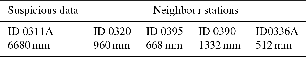
The flagged data (suspicious values) were then manually checked in their original sources (books) to discard digitization errors, in which case they were corrected, and if not they were compared against three or four neighbouring stations to decide whether to maintain or discard them. An example of data rejection is provided in Table 1.

Table 1 Example of an anomalous value discarded by comparison with their nearest neighbours (December of 1920).

2.2 Spatial interpolation (two-step method)

We use geostatistical techniques for the interpolation of monthly precipitation. Geostatistics is now a well-known field, and it has been presented in a wide range of introductory texts (Goovaerts, 1997), so we should provide only a brief summary here. The key element in geostatistics is the variogram (or, more commonly, the semivariogram), which is a function that relates the semi-variance γ between any pair of measurements to the spatial distance between them, h:

$$\begin{array}{}\text{(1)}& \mathit{\gamma }\left(h\right)={\displaystyle \frac{\mathrm{1}}{\mathrm{2}}}E\left[{\left\{Z\left(x\right)-Z(x+h)\right\}}^{\mathrm{2}}\right].\end{array}$$

An empirical semivariogram can be constructed from a set of geographically explicit measurements by analysing all the possible paired observations, and a mathematical model can then be fit to provide a continuous estimation of the relationship between any pair of points. This function can then be used to derive interpolation weights, being the basis of a family of interpolation methods known as Gaussian process regression or, in the geostatistical literature, kriging. Kriging interpolation yields best linear unbiased predictions (BLUPs) at unsampled locations, being a major reason for its widespread use.

The most frequently used form of kriging is ordinary kriging (OK), in which the interpolated values are linear weighted averages of the n available observations, z(x), and an unknown constant value, Z(x₀):

$$\begin{array}{}\text{(2)}& \widehat{z}\left(x\right)={\sum }_{i=\mathrm{0}}^n{\mathit{\lambda }}_{i}z\left(x_i\right)-Z\left(x_{\mathrm{0}}\right),\end{array}$$

where λ_i are the interpolation weights, with the condition that they sum to 1 (${\sum }_{i=\mathrm{0}}^n{\mathit{\lambda }}_i)$, so the interpolation is unbiased. Although kriging does not require any distribution assumptions on the data, OK relies on second-order stationarity. That is, it is assumed that the expected value of Z(x₀) is constant over the spatial domain ($E\left[Z\left(x_{\mathrm{0}}\right)\right]=\mathit{\mu }\left(x\right)=m)$ and that the covariance for any pair of observations depends only on the distance between them ($E\left[\left\{Z\left(x\right)-m\right\}\left\{Z\left(x+h\right)-m\right\}\right]=c\left(h\right))$.

Here we used two extensions of OK, universal kriging (UK) and indicator kriging (IK). Universal kriging relaxes the first assumption and allows a spatially non-stationary mean to be dealt with, sometimes called a spatial trend. The interpolated values thus consist of a deterministic part (the trend), μ(x), and a stochastic part or residual, ρ(x):

$$\begin{array}{}\text{(3)}& \widehat{z}\left(x\right)=\mathit{\mu }\left(x\right)+\mathit{\rho }\left(x\right)={\sum }_{k=\mathrm{0}}^m{\mathit{\alpha }}_k{f}_k\left(x\right)+{\sum }_{i=\mathrm{0}}^n{\mathit{\lambda }}_{i}z\left(x_i\right),\end{array}$$

where f_k(x) are spatially varying variables and α_k are unknown regression coefficients. Therefore, UK allows for the inclusion of co-variables as predictors for the interpolation and can therefore be viewed as a mixed-effect model or a combination of regression and interpolation.

Indicator kriging, on the other hand, is useful for binary variables (event/no event) and provides an estimation of the transition probability. It uses an indicator function to transform the variable into a binary outcome instead of working with the original variable, yielding event probabilities as a result, $\widehat{p}\left(x\right)=\widehat{p}\left(z\left(x\right)=\mathrm{0}\right)$. IK can be based on either OK or UK, accepting co-variables as spatial predictors in the latter case.

Here we adopted a two-step approach, consisting of using IK for predicting precipitation occurrence and UK for predicting the precipitation magnitude. This is an approach most commonly used for the interpolation of daily precipitation (Hwang et al., 2012; Serrano-Notivoli et al., 2019) and less so for monthly data. In the case of our study area, as we will see later on, the frequency of zero-precipitation months is not irrelevant, so a two-step approach was advisable. Therefore, in a first step we used the following indicator function to transform the observed variable in millimetres into zero-precipitation events:

$$\begin{array}{}\text{(4)}& I\left(x\right)=\left\{\begin{array}{cc}\mathrm{1}& \mathrm{if}z\left(x\right)=\mathrm{0}\\ \mathrm{0}& \mathrm{otherwise}\end{array}\right..\end{array}$$

Then, we used indicator kriging to obtain estimated zero-precipitation probabilities, $\widehat{p}\left(x\right)$. In a second step we used universal kriging for estimating precipitation magnitude, $\widehat{z}\left(x\right)$. Once the two predictions were performed, we combined them into a single estimated precipitation field z^′(S) according to the following rule:

$$\begin{array}{}\text{(5)}& z^{\prime }\left(x\right)=\left\{\begin{array}{cc}\mathrm{0}& \mathrm{if}\widehat{p}\left(x\right)\le p_{\mathrm{t}}\\ \widehat{z}\left(x\right)& \mathrm{otherwise}\end{array}\right.,\end{array}$$

where $p_{\mathrm{t}}\in (\mathrm{0},\mathrm{1})$ is a classification threshold. Determining the classification threshold is a complex task, since different values can be used that lead to better performance on the event of interest (zero monthly precipitation, in our case) at the cost of allowing more false negatives, or the opposite. We shall discuss the classification in the Discussion section of this article.

We used five co-variables for the deterministic part: the easting and northing coordinates, the altitude, the distance to the coastline (Fig. A1), and the monthly climatology: zero-precipitation probability for IK (Fig. A2) and mean precipitation for UK (Fig. A3). To obtain the climatologies we computed spatial fields of monthly mean precipitation using UK and the geographic covariates mentioned above, based on data from a sample of 1698 observatories with at least 35 years of data over the period 1961–2000. This period was selected because it contained the highest number of serially complete data series, while encompassing a long enough period (40 years) to allow for stable average values of the two variables of interest. In the Discussion section we provide a comparison of this approach using the original data and using a full normalization. All co-variables were re-scaled to a common range between 0 and 1 to facilitate model parameter fitting.

One peculiarity of the variable of interest (monthly precipitation) is that it can only take non-negative values. Also, when a number of observations are considered over a sufficiently large area, the data often show a skewed distribution. One common solution to both issues is to use a logarithmic transformation of the data, i.e. interpolating on ln (x) instead of x, an approach that is sometimes known as lognormal kriging in the geostatistics literature. This generates additional issues, though, as this approach tends to overestimate lower precipitation and underestimate high precipitation (Roth, 1998). Another drawback is that it does not allow us to interpolate observations of zero precipitation, which is sometimes solved by adding a small offset, for example, interpolating on ln (x+1), although this has other undesired effects, and it does not provide a good estimation of zero observations. Here we opted for using the original variable, i.e. without a log transformation, although we compare both options in the discussion section.

Another transformation that is often applied when interpolating precipitation fields, especially with weighted averaging methods, is to transform the original values to anomalies. This is in fact a way of normalizing the data in space, as it eliminates the differences that occur between locations that systematically tend to receive much higher or lower precipitation. As new observatories appear and disappear around a given point, this could lead to biases in the interpolation that could introduce anomalies in the interpolated series. Here we decided to use anomalies computed as ratios to the long-term climatologies (mean values) computed above.

Selection of the semivariogram model and parameter fitting are fundamental steps for kriging. There are many different semivariogram models available, and there is no general rule as to how to choose one over the other but the modeller's experience. While some models offer greater flexibility to adapt to the empirical semivariogram, parameter estimation can become a problem in some cases because there are no exact solutions, and the iterative algorithms used do not always yield good results. This is usually not a problem when performing one interpolation as the analyst often tries different options and checks that there are no substantial differences between the results, but it can be an issue when a large number of interpolations need to be done and an automatic process needs to be designed, as was the case here. We used the function krige from the gstat package for R (Pebesma, 2004; Gräler et al., 2016) to perform the kriging interpolations and autofitVariogram from the package automap (Hiemstra et al., 2009) to compute the semivariogram coefficients. The Matérn semivariogram model was the most frequently selected one, both for indicator and universal kriging. It is a highly flexible model that often yields optimum results. In some cases, though, a Gaussian model was preferred by the automated procedure, and in a few cases the automatic process was not able to converge to good parameter values, so a spherical or an exponential (less flexible but more robust) model was enforced. The frequency of each semivariogram model over the whole time period is provided, for IK and UK, in the additional material (Table A1).

Best linear unbiased predictions (BLUPs), characterized by their mean and standard deviation, were then cast over a point grid at regular distance over longitude and latitude, with a mean distance of 10 km between points.

2.3 Evaluation

Evaluation of the interpolation results is fundamental to fully understand the benefits of the interpolated dataset, the limitations, and the best use cases. Here we performed a thorough evaluation based on several statistics and checks, for both the IK (probability of zero precipitation) and the UK (precipitation magnitude) interpolations. To evaluate the performance of the interpolation method to estimate values at unmeasured locations, we followed a leave-one-out cross-validation (LOOCV) approach. This is an iterative process in which the interpolation is repeated as many times as there are data, each time removing one observation from the training dataset that is later used to compare the estimated and observed values. Although this is a time-consuming process, it allows us to obtain an independent sample that better represents the ability of the model to estimate values when no data are available. By not removing other observations that the one being used for evaluation, we could also test the effect of having a varying number of observations in the vicinity.

There is no consensus about the most appropriate statistic to evaluate binary classifications and their associated confusion matrices. A confusion matrix, also known as an error matrix, has four categories: true positives, TP (pred =0, obs =0); true negatives, TN (pred >0, obs >0); false positives, FP (pred =0, obs >0); and false negatives, FN (pred >0, obs =0); and the total positive (P) and negative (N) observations and the positive and negative predicted totals (PP = TP + FP and PN = TN + FN, respectively). A variety of statistics can be calculated based on these quantities, of which here we focused on the following ones.

• The positive prediction value (PPV) is the fraction of positive predictions that are true positive: $\mathrm{PPV}=\mathrm{PP}/\mathrm{TP}$.

• The negative predictive value (NPV) is the fraction of negative predictions that are true negative: $\mathrm{NPV}=\mathrm{NP}/\mathrm{TN}$.

• The true positive rate (TPR) is the fraction of positive cases correctly predicted: $\mathrm{TPR}=\mathrm{TP}/(\mathrm{TP}+\mathrm{FN})$. It can be considered the probability of detection (if a case is positive, the probability that it would be predicted as such).

• The true negative rate (TNR) is the fraction of negative cases that were correctly predicted: $\mathrm{TNR}=\mathrm{TN}/(\mathrm{TN}+\mathrm{FP})$. It can be considered a measure of how specific the test is (if a case is negative, the probability that it would be predicted as such).

The PPV and NPV are not intrinsic to the test as they also depend on the event's prevalence (fraction of positive cases in the observed sample). In a highly un-balanced sample, such as the case of zero precipitation in our dataset in which the proportion of station/months with zero precipitation is very low, these two statistics will be highly affected. The TPR and TNR, on the contrary, do not depend on prevalence, so they are intrinsic to the test. In diagnostic testing the TPR and TNR are the most used and are known as sensitivity and specificity, respectively. In informational retrieval, the main ratios are the PPV and TPR, where they are known as precision and recall.

We also computed two metrics that summarize the elements of the confusion matrix, so they can be considered overall measures of the quality of the binary classification. The F1 score is computed as

$$\begin{array}{}\text{(6)}& \mathrm{F}\mathrm{1}={\displaystyle \frac{\mathrm{2}\mathrm{TP}}{\mathrm{2}\mathrm{TP}+\mathrm{FN}+\mathrm{FP}}}.\end{array}$$

As it can be seen, the F1 ignores the count of true negatives, so it places more emphasis on the positive cases (zero-precipitation months, in our case). The Matthews correlation coefficient (MCC), on the other hand, produces a high score only when the prediction results are good in all the four confusion matrix categories. It is equivalent to chi-square statistics for 2×2 contingency tables. Its value ranges between −1 and 1, with values close to zero meaning a bad performance (not higher than a random classifier), while 1 represents a perfect classification.

$$\begin{array}{}\text{(7)}& \mathrm{MCC}={\displaystyle \frac{\left(\mathrm{TP}\times \mathrm{TN}\right)-\left(\mathrm{FP}\times \mathrm{FN}\right)}{\sqrt{\left(\mathrm{TP}+\mathrm{FP}\right)\left(\mathrm{TP}+\mathrm{FN}\right)\left(\mathrm{TN}+\mathrm{FP}\right)\left(\mathrm{TN}+\mathrm{FN}\right)}}}\end{array}$$

All these statistics vary between 0 and 1, where a high value (close to 1) is interpreted as indicating a high accuracy.

For the evaluation of the magnitude we used the following metrics:

• the mean absolute error (MAE) and the relative MAE (RMAE), as global error measures;

• the mean error (ME) and the relative ME (RME), as global bias measures;

• the ratio of standard deviations (RSD), as a measure of variance deflation;

• the Kling–Gupta efficiency (KGE), as an overall goodness-of-fit measure.

Model evaluation was performed globally considering the whole dataset but also for each month individually to make it possible to analyse the temporal evolution of the performance statistics.

Finally, in order to determine the benefits of the data rescue process, we compared the original (NCDB) and augmented (NCDB+YB) datasets. We used the same cross-validation scheme described above, but in this case the validation was restricted to the period covered by the yearbooks (1916–1950). Another important difference is that we only used the observations present in both the NCDB and NCDB+YB datasets for computing cross-validation statistics, although the whole datasets were used for performing the interpolation.

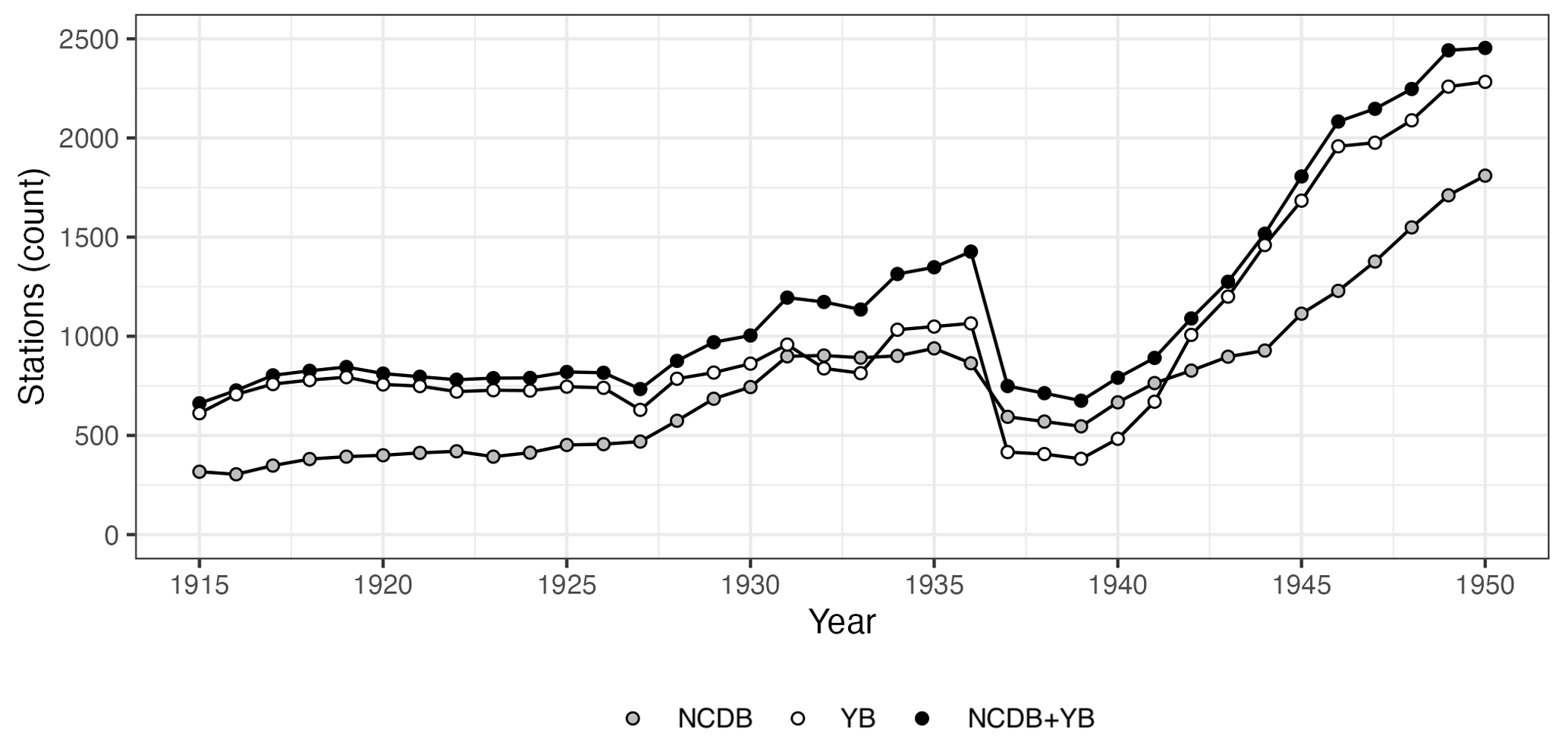
Figure 1 Temporal evolution of the number of active weather stations in the dataset: national digital data bank (NCDB), newly digitized yearbook (YB) datasets, and their combination (NCDB+YB).

3 Results

3.1 Data rescue and quality control

The annual weather yearbooks proved to be an outstanding source of climate data over the 1916–1950 period, as it contained 369 286 observations from 4248 stations, compared to 281 951 observations from 2732 stations for the NCDB in the same period. As expected, there was a significant overlap between the two sources, so the augmented dataset resulting from their combination contained 432 183 observations from 4414 stations. Figure 1 shows the temporal evolution of the two datasets and their combination over 1916–1950. With the exception of a few years (1932, 1933, and 1937–1941), the yearbooks vastly surpassed the NCDB in number of active stations. The improvement of the combined dataset with respect to the NCDB ranged between more than 100 % before 1920 and between 80 % and 20 % in the remaining of the period.

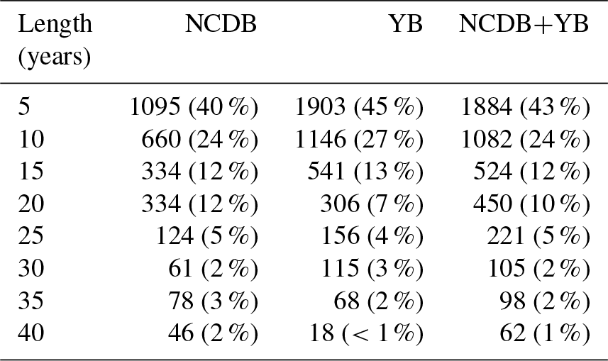
A striking characteristic of the dataset during this first period was the abundance of short-lived time series and even more so in the yearbooks' data (Table 2). The highest frequency (43 %) corresponds to series with less than 5 years of data, while 65 % of the series had no more than 10 years. On the other hand, less than 5 % of stations cover the complete period 1916–1950.

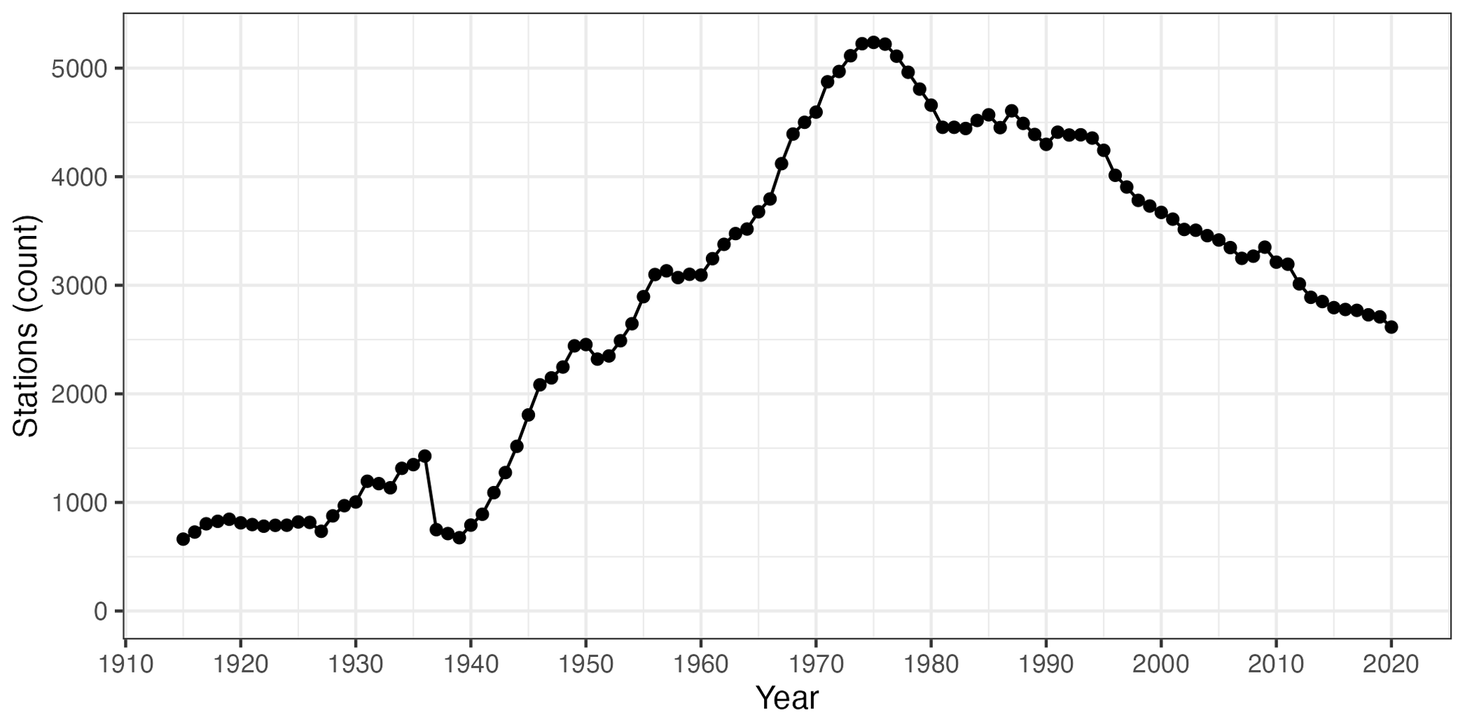
Figure 2 Temporal evolution of the number of active weather stations in the dataset over the whole study period.

Table 2 Number and percentage of stations according to the length of the record, for the period 1916–1950.

The complete dataset, spanning 1916–2020, contained more than 3.3 million records from 11 008 weather stations. The number of stations currently active in any given year was much lower, though, and it varied significantly (Fig. 2). After a first decade (1916–1925) with no large variation at around 800 active stations, the number of active stations increased steadily, reaching approximately 2500 stations in 1950 and peaking at 5237 in 1975. The number of active stations has progressively decreased since, reaching 2615 in 2020. The most notable exception to this general trend was the Spanish Civil War period between 1936 and 1939 and the immediate post-war years, when the dataset was severely reduced and reached its lowest count at 675 active stations in 1939.

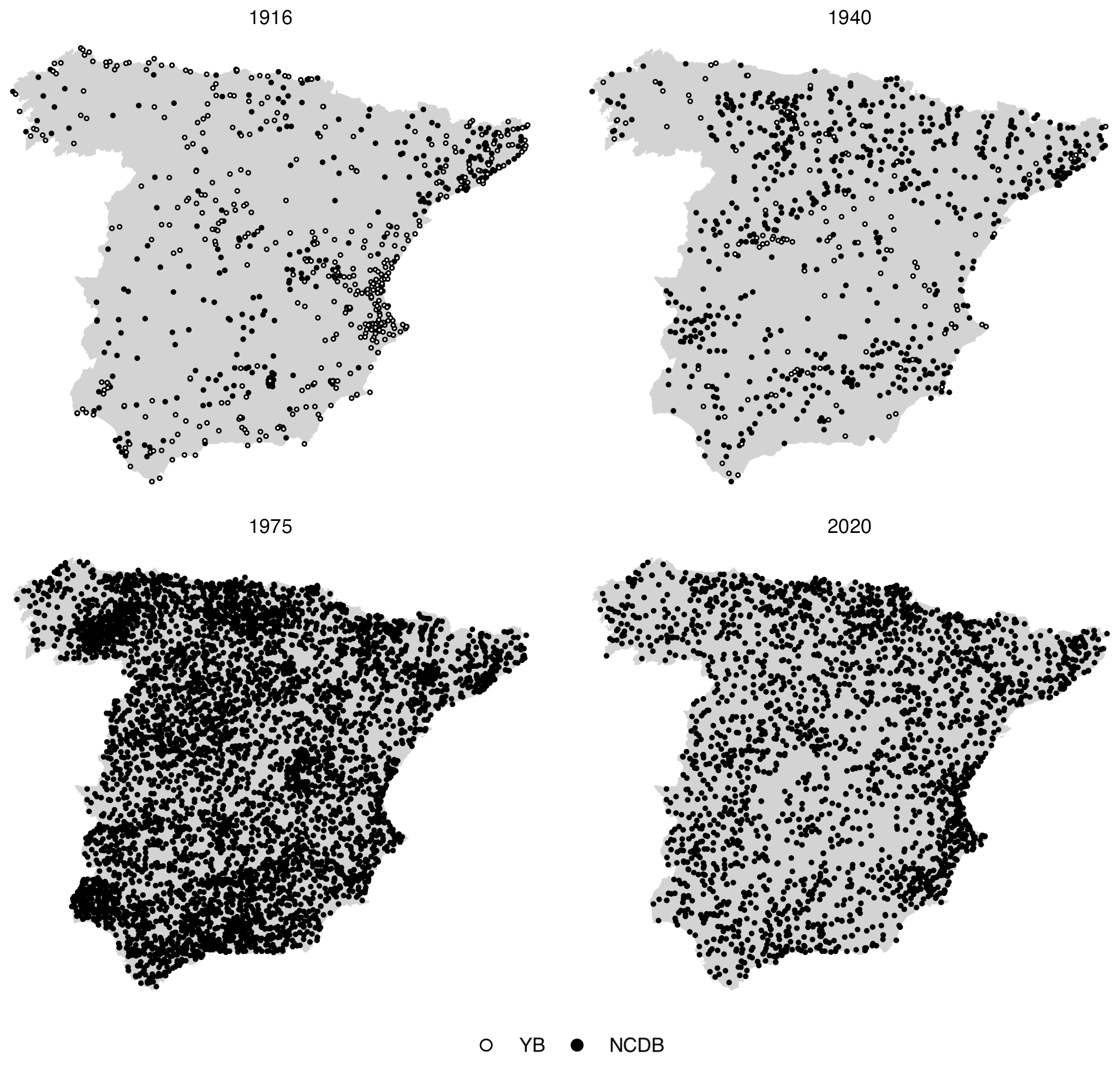
Figure 3 Spatial distribution of the weather stations in selected years, with indication of the data origin.

As a consequence of this variation, the information spatial density has greatly changed over time, too (Fig. 3). Also, and in particular in the first half of the 20th century, the spatial coverage of the dataset is not homogeneous as some regions have a notably lower information density. Regarding the spatial coverage, the image illustrates that the addition of the rescued data (YB dataset) improved the data density in some regions that were severely under-represented in the original dataset (NCDB), such as the south-west (Guadalquivir River basin), in a significant way.

As temporal changes in data availability can have an impact in the interpolation results and in any ulterior analysis, we assessed them in more depth. Figure 4 informs on the evolution of the distance to the closest neighbouring station (mean and standard deviation). Since the random component of kriging is essentially a distance-based weighting scheme, this is a relevant statistic that is related to the degree of spatial smoothing introduced by the interpolation. Prior to 1940 the mean distance ranged between 10 and 12 km, rapidly decaying to less than 6 km after 1960. The minimum average distance (5.9 km) was achieved in 1973, with a slight increase since then up to the present. Interestingly, the increase of the closest neighbour distance in recent years has been slower than the reduction in the number of observatories, evidencing a more even spatial distribution of the observation network that is also apparent when the spatial distribution of the stations in 2015 and 1955 are compared. The effect of the reduction of stations is perhaps more evident in the distance variances. The variability of the number and density of observations during the study period is a potential source of undesired effects in the interpolated dataset, reinforcing the need for a thorough validation.

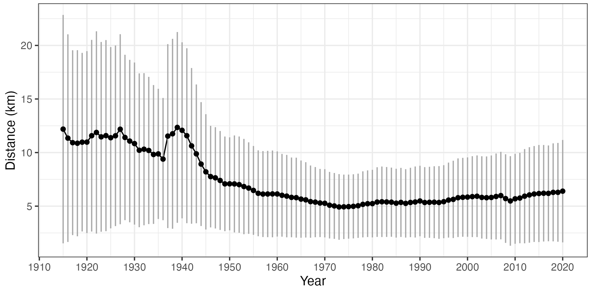
Figure 4 Temporal evolution of the distance to the closest station: mean (black dots) and 2 standard deviation range (vertical grey lines).

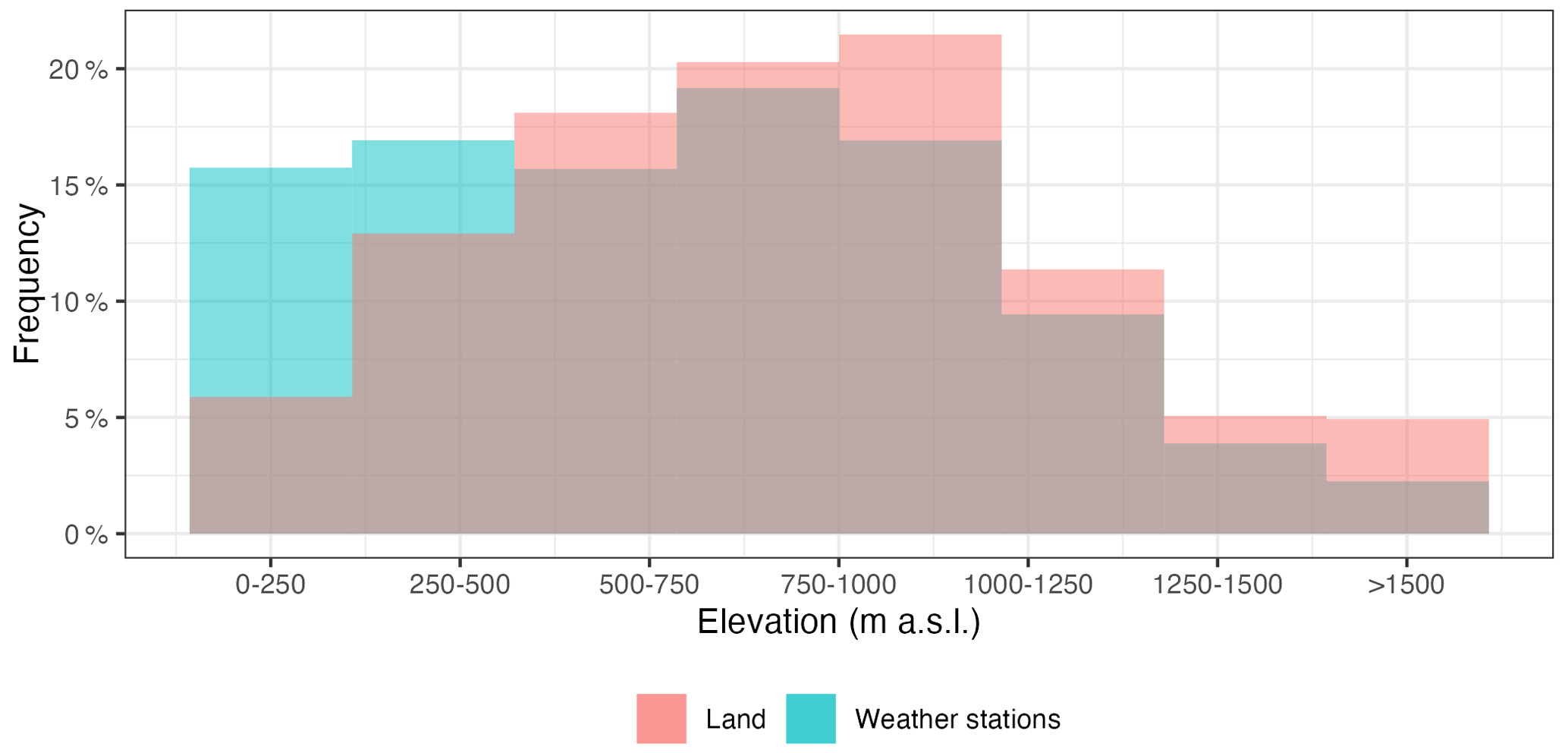
Figure 5 Frequency histogram of weather stations per elevation class, as compared to the whole study area.

Another potential source of bias arises from the altitudinal distribution of the stations, since there is usually a good correlation between monthly precipitation and elevation, so ideally the observations should sample evenly all the altitudinal ranges on the study area. In our case, the areas below 500 m a.s.l. tended to be over-represented when the proportion of observations per altitude ranges was compared to that of the study area, while higher areas were slightly under-represented (Fig. 5). Strong temporal changes in the altitudinal distribution of the stations could be an additional problem as it could generate temporal bias in the resulting grids. However, in our case the altitudinal distribution of the observations changed only slightly, with the average elevation oscillating between 575 (first quartile) and 614 (third quartile) m a.s.l., values that correspond approximately to the mean elevation of mainland Spain (Fig. 6). The relative composition of the dataset by altitudinal classes has not changed significantly over the study period, so no temporal bias was to be expected due to elevation shifts (Fig. A4).

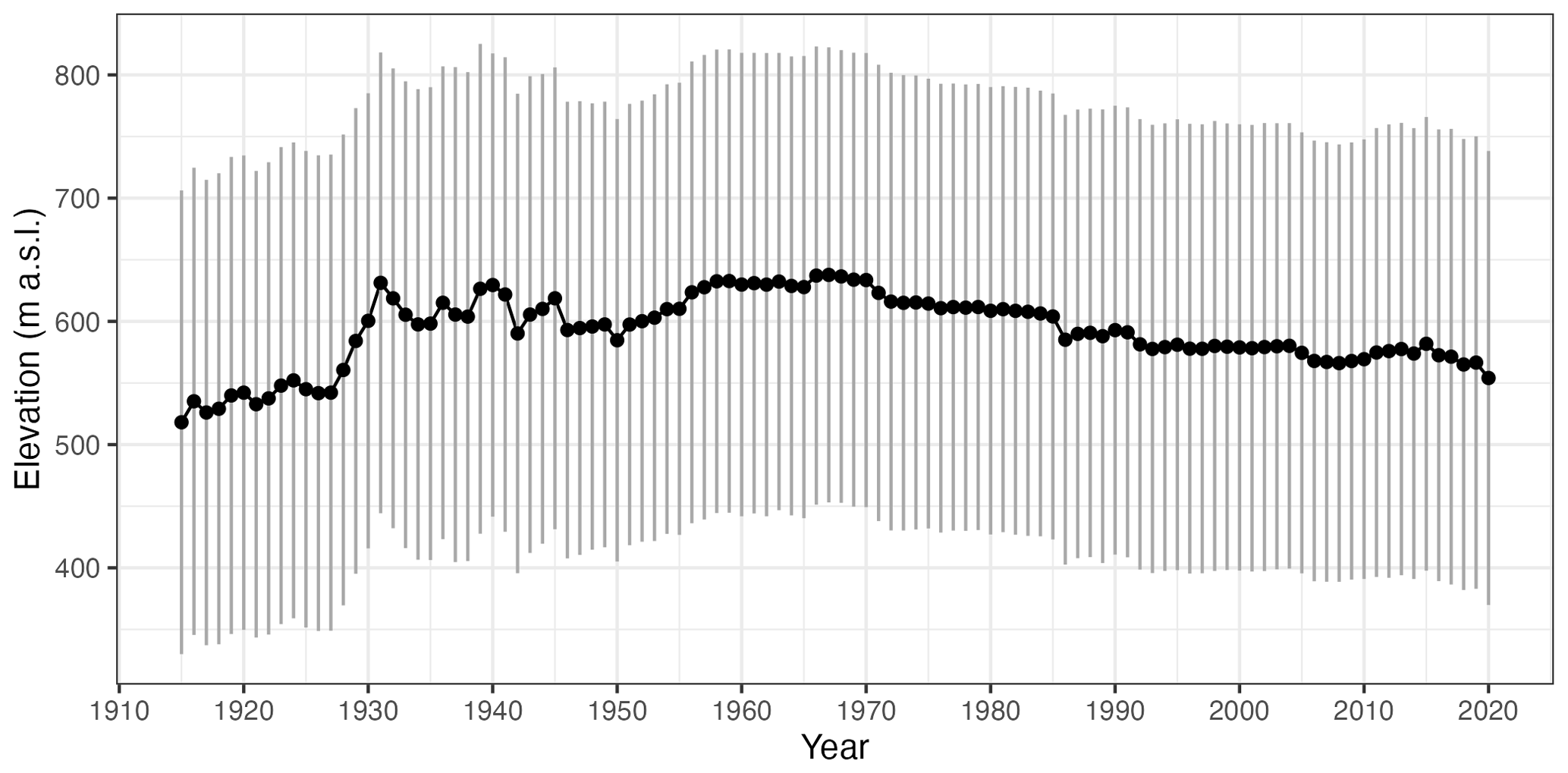
Figure 6 Temporal evolution of the station network's elevation: mean (dots) and 2 standard deviation range (vertical lines).

Table 3 Number and fraction of stations according to the length of the record, for the period 1916–2015.

Regarding the length of the data series, the frequency of observatories with less than 5 years of data is 22 %. A total of 34 % of the series cover more than 30 years, while only a few (0.1 %) cover the complete period (Table 3).

While this heterogeneity of record lengths is not uncommon in observational datasets, it imposes an important decision that conditions the development of gridded dataset: whether to use all the information available at any given moment, even if the data availability changes over time, or to restrict the analysis to a reduced set of stations that do not change over time. The last option implies selecting the largest and most complete data series and then undergoing a gap-filling and reconstruction process, in order to make all the series cover the whole period of study, at the cost of rejecting a large amount of valid data and the risk of introducing statistical artefacts during the reconstruction process. The first option, on the other hand, has the advantage of making use of all the information available but the risk of introducing statistical biases in the dataset since the number of observations change largely over time. We shall discuss this issue later in the article.

Table 4 Monthly distribution of anomalous data discarded during the quality control: number of observations and percent over the whole data.

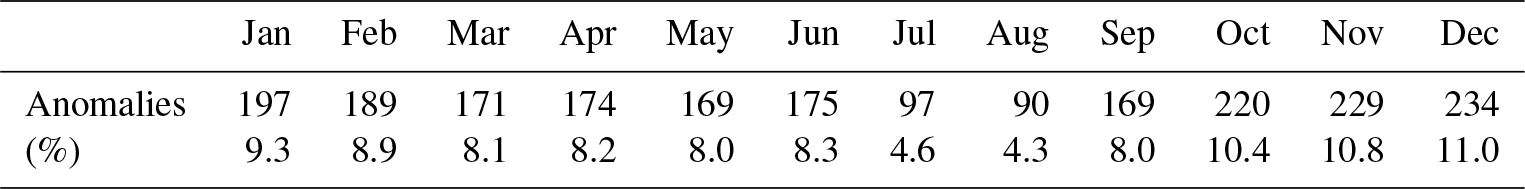
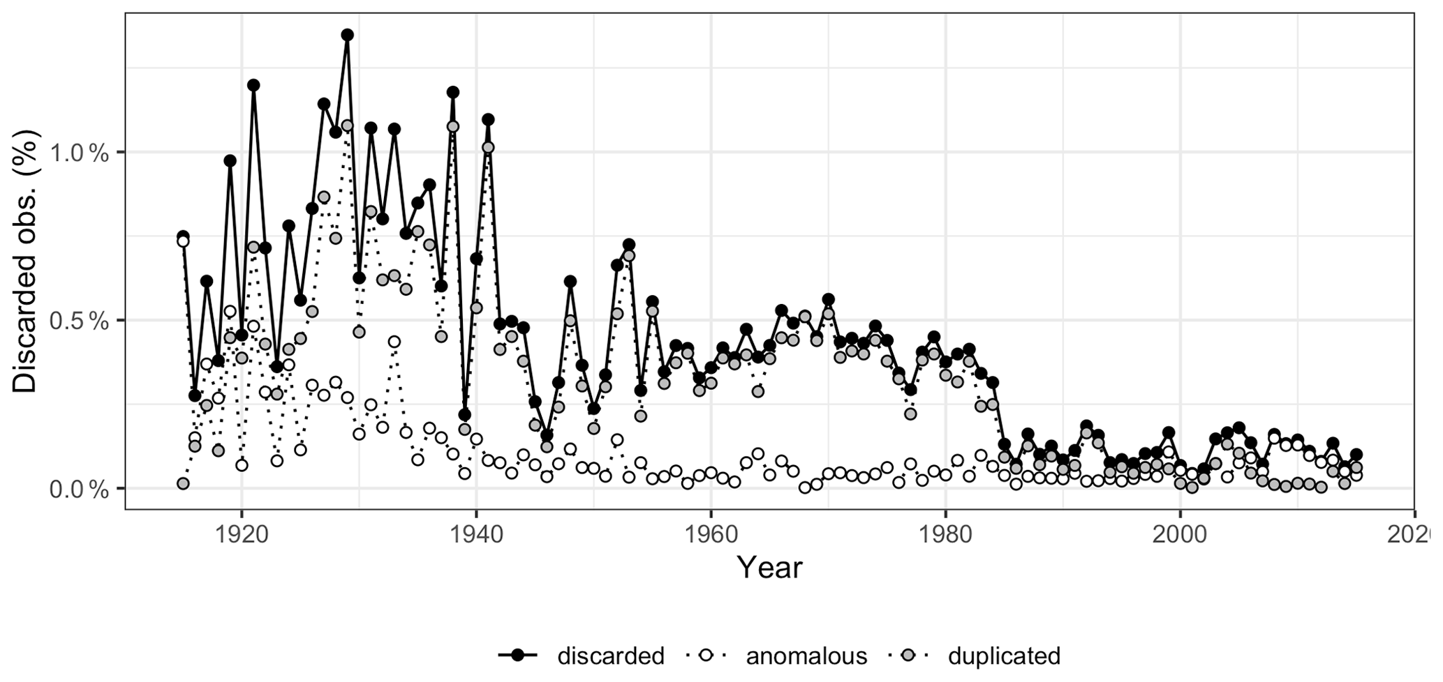
Figure 7 Temporal evolution of the observations discarded during quality control (percent per year), according to the reason: duplicated data, anomalous values, and total discarded.

Figure 7 shows the time series of data discarded during the quality control process. Discarded data amounted to 0.5 %–1 % of the records prior to 1940, between 0.25 %–0.5 % during 1940–1985, and lower than 0.2 % since ∼1985. The largest part of the rejections was due to repeated sequences in the same station or between different stations in the same year, while anomalous data (sequences of zeros or extremely high values) amounted for a much lower proportion or rejections. Discarded data are distributed evenly across the year (Table 4), with a certain lower prevalence in July and August that might be due to the higher difficulty to detect anomalies during those months given the more irregular character of precipitation.

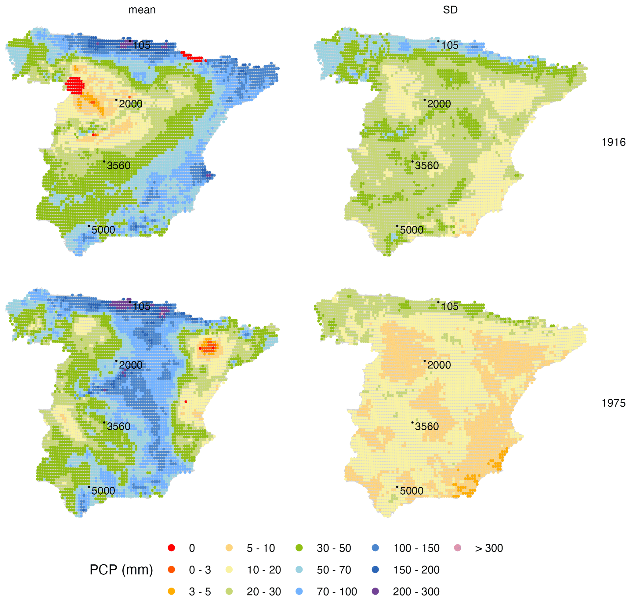
Figure 8 Example grids: mean and standard deviation of monthly precipitation (PCP) best linear unbiased predictions (BLUPS) for April 1916 (up) and April 1975 (bottom). Black dots and numbers identify the location of four random points selected for further analysis.

3.2 Gridded dataset

The result of the interpolation process was a gridded database of mean and standard deviation fields of the best linear unbiased predictions (BLUPS) of monthly precipitation between January 1916 and December 2020 (1272 time steps). As an example of the dataset, mean and standard deviation fields are shown for April 1916 and 1975 (Fig. 8). The figures illustrate the probabilistic nature of the Gaussian process interpolation, as the mean and standard deviation fully describe the probability distribution of estimated precipitation at each point of the grid. There is a noticeable difference in the observational data density leading to each interpolated grid (as seen in Fig. 3), which had an impact mainly on the magnitude of the standard deviation field. In fact, despite a similar range of the mean predicted values, the standard deviation field value ranges were very different between the two dates, being almost double in 1916 than in 1975, revealing a higher uncertainty of the estimated values.

Figure 9 Time series of best linear unbiased predictions (BLUPs) of April precipitation at four random grid points (left column): means (black dots) and 2 standard deviation range (vertical lines), standard deviation of the predictions (central column), and mean distance to the nearest observation (right column).

This is further illustrated in Fig. 9 (left panel), which shows time series of estimated monthly precipitation (BLUPs) with their uncertainty levels (±1 standard deviation) at four random grid points. In addition, time series of the standard deviation and of the distance to the closest observation are also provided. Two facts are apparent upon inspection of the plots: (i) there is a linear relationship between the predicted precipitation and the uncertainty range (i.e. there is a larger uncertainty for higher precipitation), and (ii) there is a reduction of the uncertainty range with time, which can be related to the progressive addition of new information.

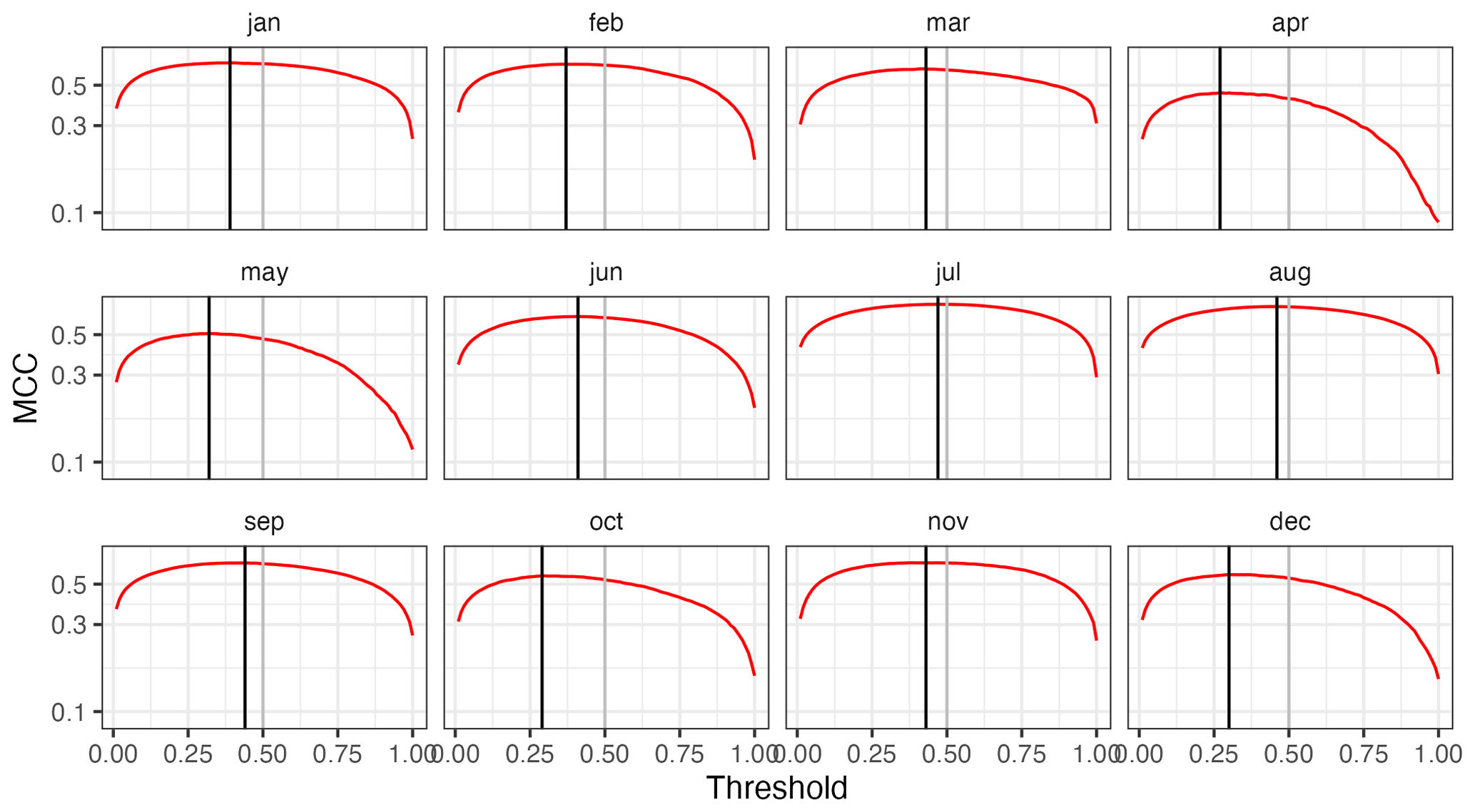
Figure 10 Selection of zero-precipitation prediction thresholds based on the MCC statistic (cross-validation results).

3.3 Validation: probability of zero precipitation

The MCC statistic was used to determine the classification threshold for the interpolation of precipitation occurrence, since it provides a good balance between the prediction of positive and negative cases (Fig. 10). Classification thresholds were computed for each month and were applied globally (i.e. the same thresholds applied for the whole spatial and temporal domains). The threshold values were lower in winter (close to 0.25) and higher in summer (close to 0.50), reflecting the seasonal variation of the prevalence of zero precipitation. The thresholds offered a good balance as they tended to maximize the individual metrics of the confusion matrix (Figs. A5 and A6).

As a result, a reasonably good prediction of zero-precipitation cases was obtained in the summer months, when the prevalence is higher and thus more important, while during the rest of the year, when the prevalence is lower and therefore less relevant, there was a slight underestimation of zero-precipitation cases (Fig. 11).

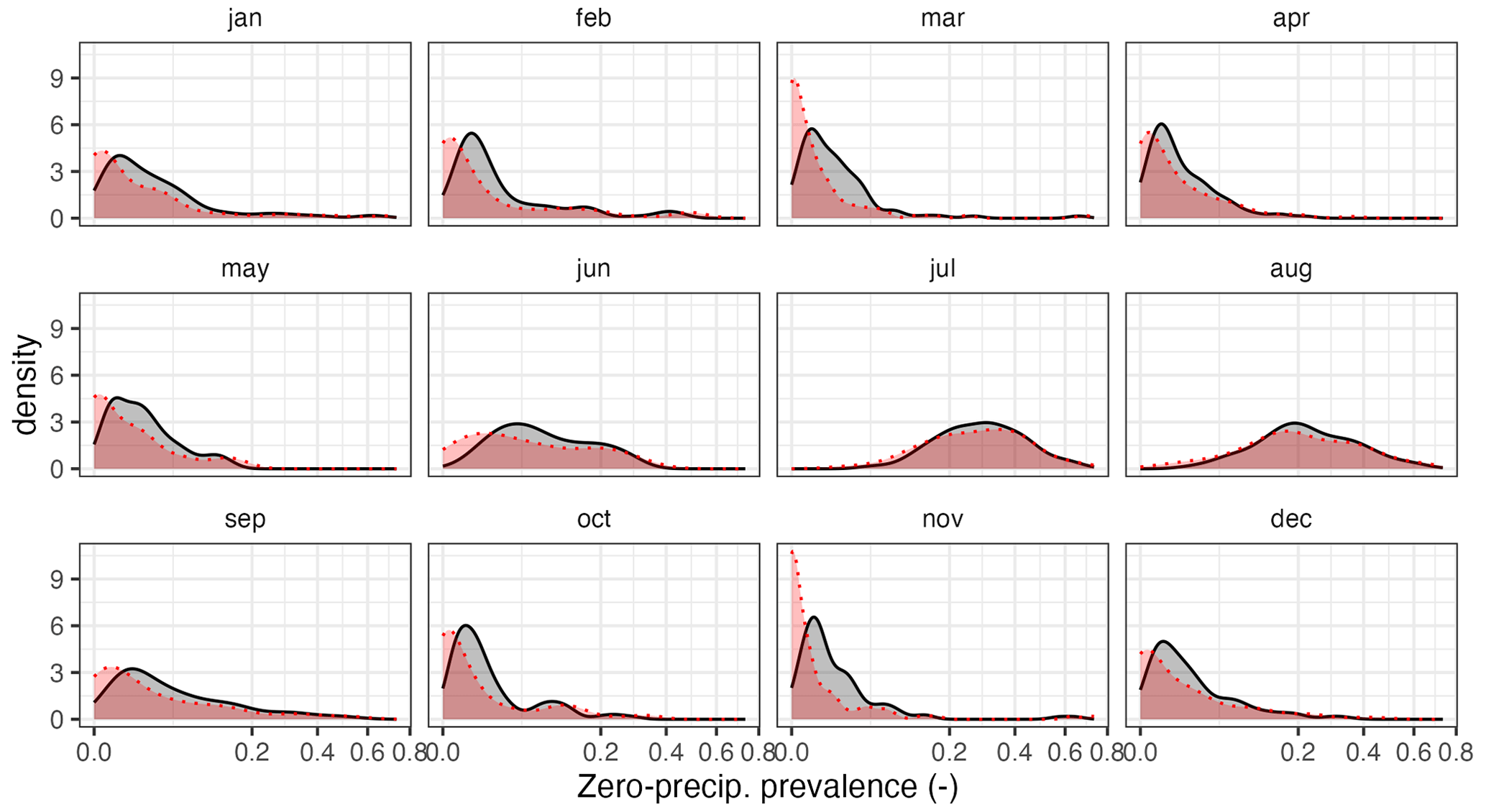
Figure 11 Empirical density functions of zero-precipitation frequency in the observed (grey) and cross-validation (red) datasets.

Table 5 Cross-validation statistics for zero-precipitation estimation: true positive ratio (TPR), true negative ratio (TNR), positive predictive value (PPV), negative predictive value (NPV), F1 score (F1), and Matthew's correlation coefficient (MCC). Median values across all the stations.

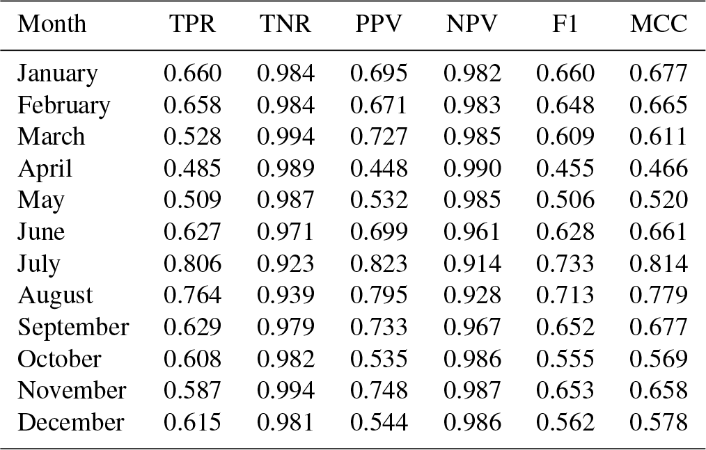
A detailed inspection of the evaluation statistics for the prediction of zero precipitation (Table 5) reveals that the interpolation was better at predicting negative cases (precipitation higher than zero) than positive cases (zero precipitation), as shown by higher TNR and NPV values over TPR and PPV. This is also reflected by the F1 score, which focuses on the ability to predict positive cases and had values in the 0.50–0.65 range for most months. Only during the summer months (especially July and August) was the skill higher.

Table 6 Mean monthly observed (obs) and predicted (pred) percentiles and mean values (cross-validation results).

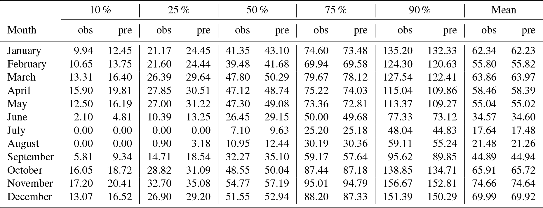
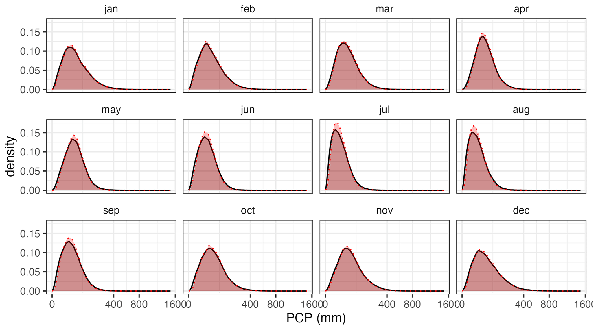
Figure 12 Density of observed (grey) and predicted (red) monthly precipitation (cross-validation results).

3.4 Validation: magnitude

Cross-validation results of precipitation magnitude (considering the combined result of the two interpolations by application of Eq. 5) can be considered good. The probability density of the interpolated values matched that of the observations quite well (Fig. 12), although the predicted values tended to be slightly more concentrated around the mode of the distribution, while under-representing the lower and higher tails of the distribution. Such variance contraction should be expected in any interpolation process, and it is more important to check for biases and temporal inconsistencies.

This can be seen in more detail when comparing the quantiles of the observed and predicted sets (Table 6). Starting by the median (50 % percentile), there was a very good match between both sets, albeit a slight overestimation can be found in most months. When considering the lower quantiles (25 % and, especially, 10 %), the overestimation is more evident, while the higher quantiles (75 % and, especially, 90 %) show a closer match.

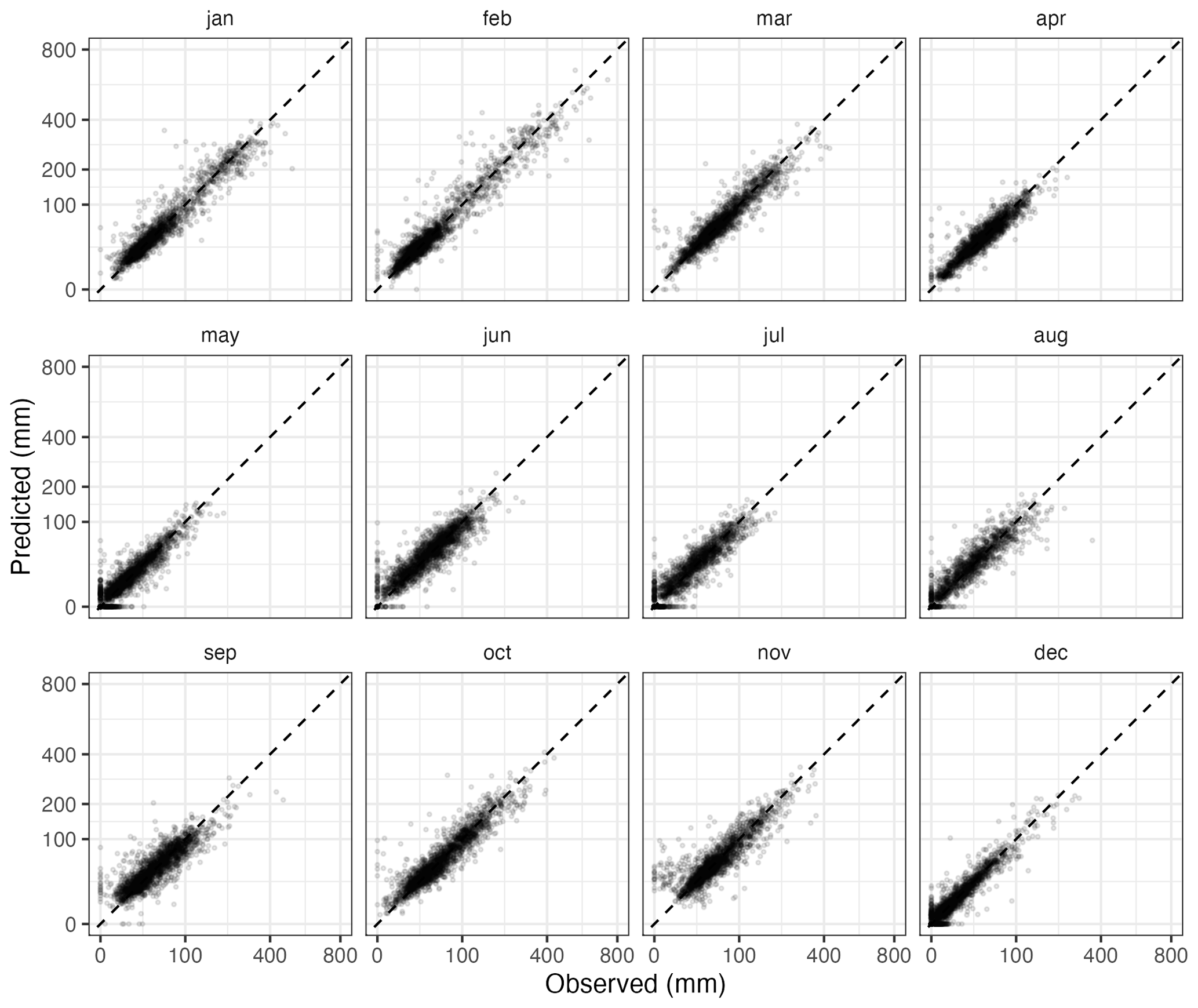
Figure 13 Predicted and observed monthly precipitation values for the year 2015 (cross-validation results). Each dot represents one weather station.

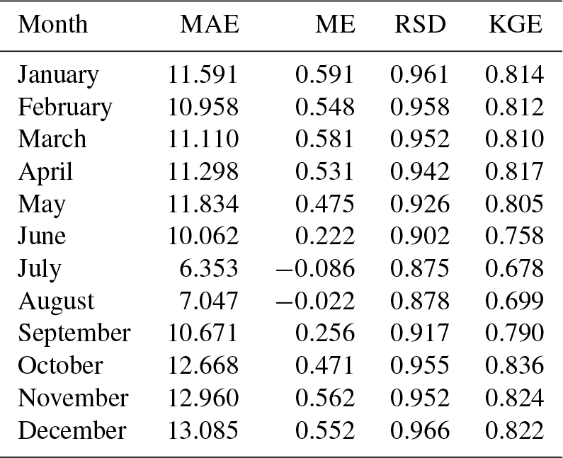
Table 7 Cross-validation statistics for precipitation magnitude estimation: mean absolute error (MAE; mm), mean error (ME; mm), ratio of standard deviations (RSD), Kling–Gupta efficiency (KGE). Median values across all the stations.

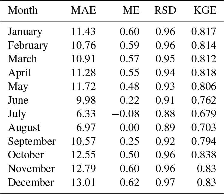
Cross-validation statistics for the magnitude interpolation are given in Table 7, and an example scatter plot of predicted against observed values for a 12-month period is provided in Fig. 13. The MAE over the whole dataset ranged between slightly less than 7 mm in July and 17 mm in December. These might seem to be quite high error values, but it must be kept in mind that the distribution of the variable of interest is highly skewed, so a relatively low number of very high observations contributes a lot to the statistic. In fact, visual inspection of the scatter plots in Fig. 13 reveals a good match between observations and predictions, in all months.

The ME, very close to 0 mm, indicates no significant bias in the predictions. The RSD was in general close to 0.9, which can be considered a good result and implies only a slight reduction of the spatial variance in the predicted precipitation fields. The KGE, finally, was quite good, too, with values ranging between 0.79 in May (worst case) and 0.85 in December–January (best months). In general, the validation results were better in winter and worse during the summer months.

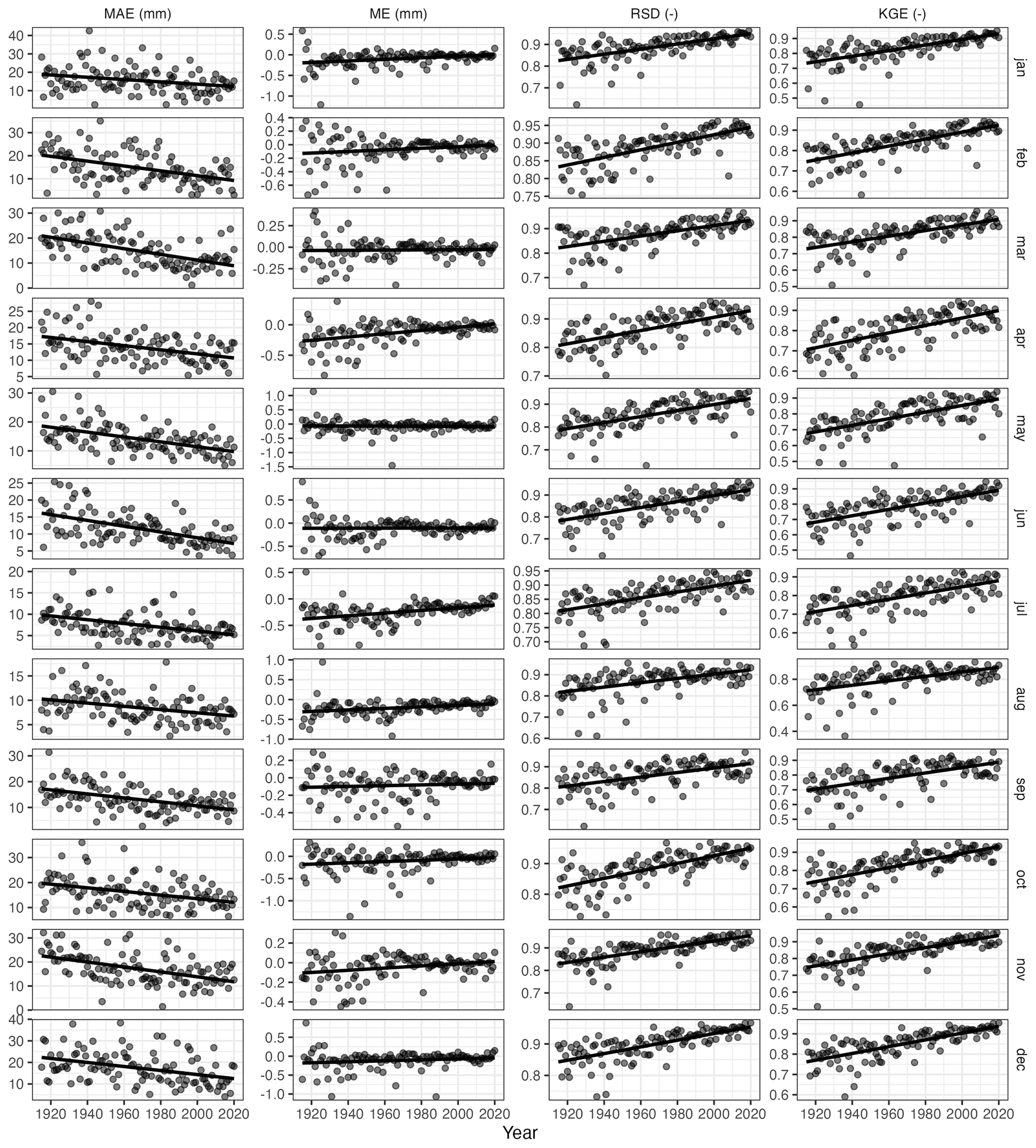
Figure 14 Temporal evolution of the mean absolute error (MAE), mean error (ME), ratio of standard deviations (RSD), and Kling–Gupta efficiency (KGE) for each month (cross-validation results).

A very important issue when constructing gridded datasets over an extended period, as was the case here, is to consider potential biases that may arise from the substantial change in the number of observations available at different times. Large temporal variation in the size of the observational dataset can potentially impact several aspects of the interpolated grids, mostly their spatial variance, and even might be a source of bias. Here we checked for such changes by computing cross-validation statistics for each monthly grid independently and then inspecting the time series of said statistics, looking for temporal trends (Fig. 14). Ideally, validation statistics should be time-stationary, although some effects are inevitable due to the changes in the size of the observational dataset.

The first and most obvious consequence of the variation in the number of observations is the effect on the overall accuracy, as expressed by the MAE. As the size of the observed dataset increased over time, the absolute error of the interpolation also decreased. A similar result would be obtained by inspecting the evolution of other goodness-of-fit statistic, such as the R², and is an inevitable consequence of having more data to interpolate. In our case, the reduction of the MAE was approximately 2-fold; that is, the error was 2 times higher during the first decades of the 20th century, when the observational data were scarcest, than during the last decades of the study period.

More relevant than the absolute error is the evolution of the mean error, as it informs about possible systematic temporal biases that could affect, for instance, the computation of temporal trends using the interpolated grid. In principle, the unbiasedness of the kriging interpolation is independent of the size of the dataset, so no temporal bias should be expected. However, other factors related to the normalization of the data or other steps of the process could introduce undesired effects. In our case, the ME was stationary or only exhibited very limited temporal trend, with close-to-zero values and mostly random oscillations. Only for some months (April and July being the most conspicuous) was a slight increasing trend of the ME apparent, albeit the magnitude of the difference between the start and the end of the study period (less than 0.5 mm) was very low in comparison with the magnitude of the variable.

Another well-known effect of the sample size is that it is related to the variance shrinkage of the interpolation. This can be inspected by the RSD statistic, which showed an increasing trend as the size of the available data increased. The magnitude of the difference between the start and the end of the study period ranged around 0.1, indicating that later grids had larger variability (and much closer to that of the observed sample) than earlier grids. Despite the magnitude of the effect not being too high, it is something that should be considered, for instance, if the interpolated grid was to be used for assessing variability or extreme values changes over time.

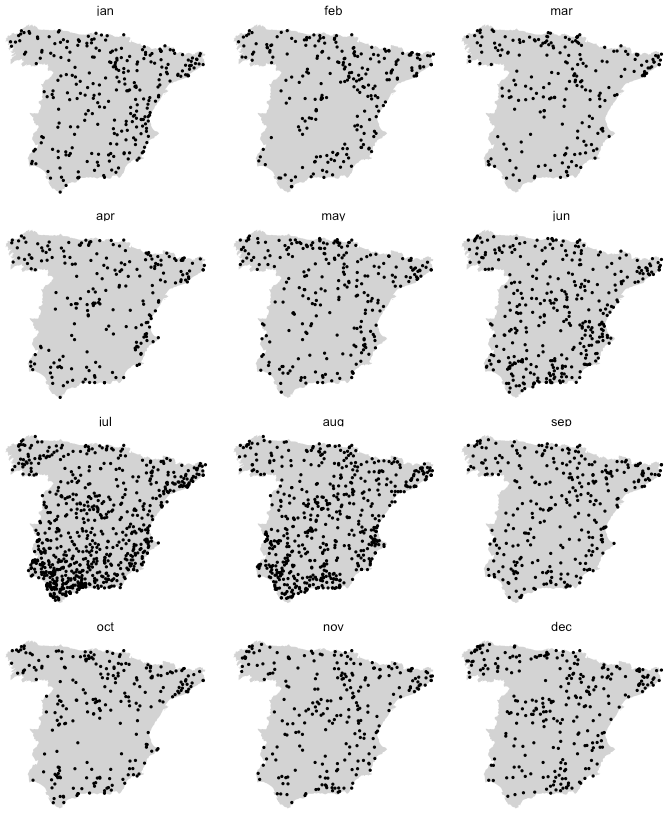
Figure 15 Location of station/months with negative KGE over the period 1916–2020 (cross-validation results).

As a final result, indicative of the overall goodness of fit of the interpolation and considering the error, the bias, and the variability, the KGE statistic showed a steady increase during the study period ranging between values in the 0.65–0.7 range at the beginning of the period and close to 0.9 at the end.

A spatial evaluation of the quality of the interpolation, focusing on the KGE statistic, shows that the worst results were obtained in the summer months and towards the south of the study area (Fig. 15).

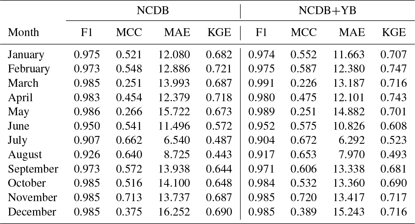
Table 8 Cross-validation statistics for zero precipitation and magnitude in the original (NCDB) and augmented (NCDB+YB) datasets: F1 score (F1), Matthew's correlation coefficient (MCC), mean absolute error (MAE; mm), and Kling–Gupta efficiency (KGE) median values across the stations, period 1916–1950.

Figure 16 Time series of the mean error in the NCDB and combined (NCDB+YB) datasets.

3.5 Evaluation of the combined dataset

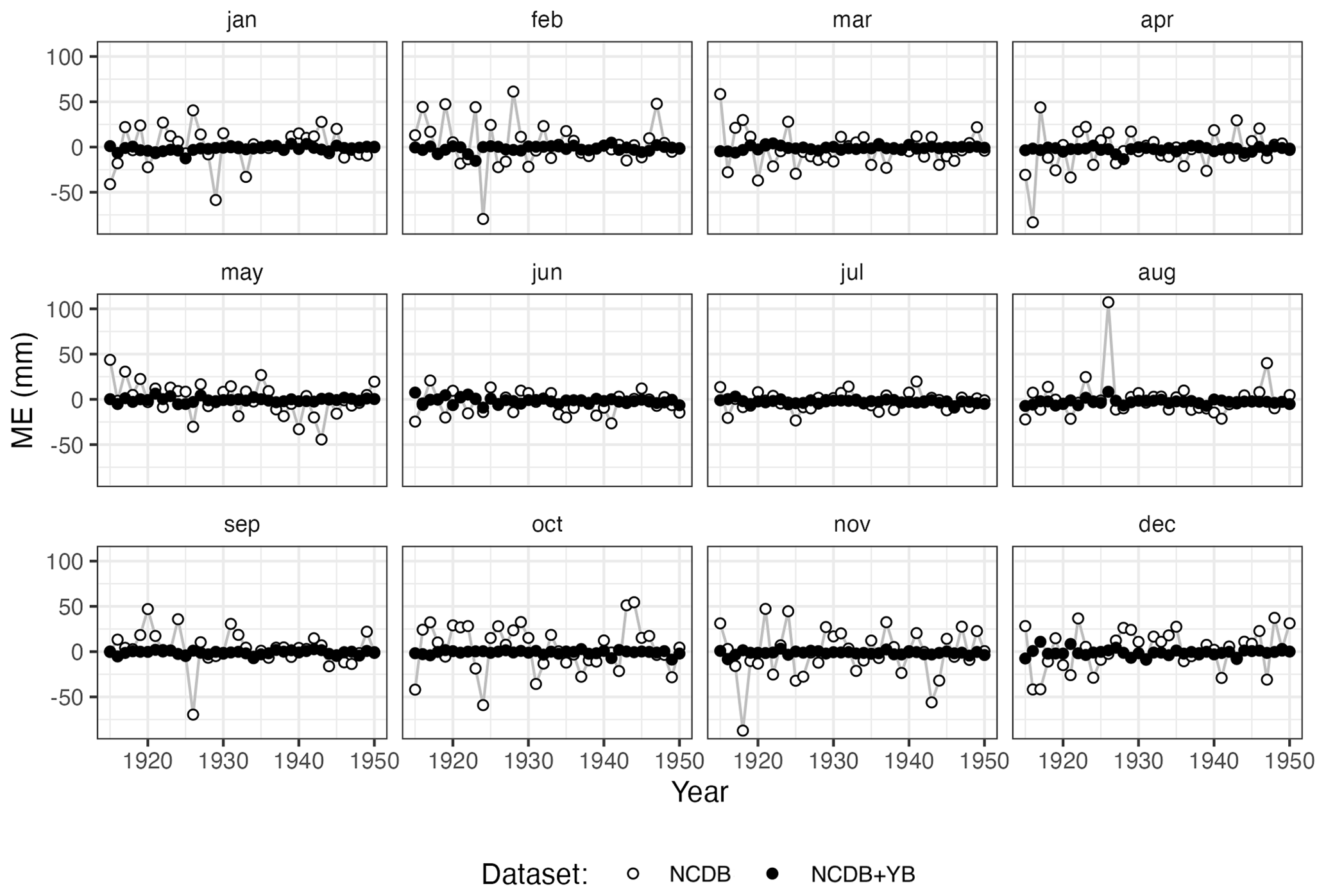
The addition of new observational data digitized from the yearbooks improved the prediction of zero precipitation and precipitation magnitude in all months, as shown by the cross-validation statistics computed over the period 1916–1950 (Table 8). The most notable improvement of the augmented dataset (NCDB+YB) over the original one (NCDB) was the stabilization of the mean error during the first decades of the study period, which exhibited large variability in the original dataset (Fig. 16).

4 Discussion

In the following paragraphs, we discuss various aspects of our spatial interpolation approach and evaluate the performance of alternative model choices. We used a geostatistical approach, universal kriging (also known as Gaussian process regression), over other well-known and used approaches such as global or local regression, and weighted averaging methods or splines, due a number of reasons. On the one hand, and similar to other regression methods, kriging performs a probabilistic prediction, as it allows not only best predictions at unsampled locations to be obtained but also their standard deviation, allowing us to determine uncertainty ranges. Under appropriate assumptions, kriging yields best linear unbiased predictions (BLUPs), unlike other weighted averaging methods that do not guarantee unbiasedness. Standard regression methods, on the other hand, only consider fixed effects and result in best linear unbiased estimations, ignoring the random part. In a preliminary phase we found that kriging resulted in better cross-validation statistics than, for instance, angular-weighting interpolation.

In order to make the best use of the data, we used all the observations available at each time step. As a result, the interpolation sample varied largely on time, as the number of weather stations available was 5 times higher at their peak in the middle 1970s than at the beginning on the period (1916–1940). Such a strong variation in the observational dataset is not uncommon when analysing large temporal periods and may have non-desired effects on the interpolated dataset, advising a thorough temporal validation. It is evident that a bigger sample would result in reduced prediction uncertainty but should not result in systematic bias. We found that to be correct, as only the MAE but not the ME was affected by temporal changes in the sample size. This implies that the interpolated dataset can be safely used for climatological analyses involving the calculation of means or trends in the mean values, over the whole temporal range or over shorter time spans. However, some unexpected temporal bias was found related to certain variable transformations, which were discarded (more on that later). Also, as it was expected, smaller samples resulted in a reduced variance (as shown by the RSD). As a result, caution is recommended when using the dataset for climatological assessments of spatial or temporal variability, extremes, or quantiles other than the mean.

A common concern that is often expressed against using a time-varying sample for interpolation is that it might introduce biases (inhomogeneities) in the predicted time series at given locations as new weather stations appear (or disappear) in the vicinity of the point, due to possible systematic differences between the two points. Although this is more problematic with weighted averaging methods than with regression or kriging approaches, we decided to use a variable transformation in order to eliminate such differences. Therefore, we transformed the original data in millimetres into anomalies (ratios to the point's long-term climatology). Although this is not a strict requirement of kriging, interpolating the anomalies and transforming back to the original units resulted in slightly better cross-validation results (Table A3) and helped ensuring the statistical continuity of the predicted time series at any given point of the grid as new observations (weather stations) appeared in the vicinity of the point.

We tried other variable transformations than the ratios to the climatology, with not quite as good results. One of the most promising approaches was performing a full standardization of the variable by converting the original values into standardized variates. In fact, converting the observed values into Standardized Precipitation Index anomalies improved the error statistics slightly (MAE), albeit it yielded worse bias statistics (ME) and overall accuracy (KGE; Table A4). The worse ME of the full standardization might be a result of the transformation of the variable, but the most preoccupying effect was that it introduced a strong temporal component in the ME (Fig. A8), with a bias magnitude that could no longer be considered irrelevant as it could appreciably alter, for instance, the computation of temporal trends based on the interpolated grid.

Another important aspect of our approach is that it consisted of two steps, where the final precipitation prediction is the result of independent estimation of the probability of zero precipitation and precipitation magnitude. This allowed a better representation of zero-precipitation areas to be attained, which was especially relevant for the summer months. As a comparison, a single-step approach (that is, direct interpolation of precipitation magnitude) resulted in a severe underestimation of zero precipitation: if the prevalence of zero-precipitation cases was 8.24 % in the observational dataset, using a single-step approach this value got reduced to 1.64 %. Our two-step approach, on the other hand, yielded a much closer estimation at 8.07 %. Underestimation was especially important during the summer, when the prevalence of zero-precipitation months is higher (Fig. A7). Using a single-step approach did not have such a remarkable impact on the prediction of precipitation magnitude, leading to similar or marginally poorer cross-validation statistics (Table A2). This came as no surprise due to the low contribution of low-precipitation values to validation statistics in general and highlights the importance of performing a thorough validation of the interpolation results that goes beyond the mere computation of error (deviation) statistics and considers other important aspects of the data, such as the prediction of zero precipitation.

We also checked the added information of using covariates, i.e. using a universal kriging approach, against a simpler ordinary kriging with no covariates. We found that the covariates resulted in better cross-validation statistics, both for the probability of zero precipitation and for magnitude, although the magnitude of the difference was not too big (Table A5).

Our variable of interest, precipitation, can only take positive values (once zero precipitation has been ruled out), and its distribution is typically skewed. In order to deal with these characteristics in a regression context, usually a logarithmic transformation of the variable is advised or the use of a logarithmic link function. However, this implies that the method's unbiasedness properties might not apply to the original variable under certain circumstances, recommending caution (Roth, 1998). Here we found that applying a log transformation to the data yielded slightly worse cross-validation results (Table A6), and, similarly to applying full-standardization, it introduced a temporal bias in the mean error. Therefore, we opted to not using this transformation.

Our approach has a number of drawbacks and potential improvements. The kriging properties rely on a proper estimation of the semivariogram model, which needs to be estimated for each time step. We found that under certain circumstances the automatically derived semivariograms were flawed (either the parameter search did not converge, or the parameters were too low or too high), so we had to put extra care into designing automated checks and solutions, as described in the methodology. Also, we found that under certain circumstances the method could be too sensitive to outlier observations.

Another important limitation is the kriging assumption of spatial stationarity, as the semivariogram model is supposed to be valid across the whole spatial domain. This is clearly a sub-optimal approach for climate variables with often complex spatial behaviour such as abrupt changes and variations in the correlation range, spatial anisotropies, etcetera. One possible solution, not explored here, is the implementation of deep Gaussian process (deepGP) regression. Unlike “shallow” kriging, as used here, deepGP introduces more than one layer of Gaussian processes and therefore allows for spatial non-stationarities to be modelled (Damianou and Lawrence, 2012), providing a promising method for the interpolation of climate variables.

Another drawback of the our approach is that, as only the information of the month being interpolated is used, a good wealth of useful information is not used. Spatio-temporal variogram models have been proposed to leverage the self-correlation properties of climatic variables (Sherman, 2011; Gräler, 2016), especially over short time periods, but other possible approaches include the use of principal components fields, weather types or k-means field classification as covariates for universal kriging. All these approaches merit exploration and will be the subject of future work.

5 Data availability

The MOPREDAScentury (Monthly Precipitation Dataset of Spain) gridded dataset can be accessed on the project's website at https://clices.unizar.es (last access: 14 June 2023) and has been reposited at https://doi.org/10.20350/digitalCSIC/15136. It is distributed under the Open Data Commons Attribution (ODC-BY) license and can be cited as Beguería et al. (2023).

6 Conclusions

We created a century-long (1916–2020) dataset of monthly precipitation over mainland Spain to serve as a basis for further climatologic analysis. To achieve that, we first augmented the current observational information in the Spanish National Climate Data Bank with new data digitized from climatic yearbooks during the period 1916–1950. This allowed the information available in the first decades of the 20th century to be almost doubled, a crucial task due to the general data scarcity during that period, especially over certain regions such as the north- and south-west of the study area. The new data helped reduce the uncertainty of the interpolated dataset and stabilized its mean error. We further used a two-step kriging method to interpolate monthly precipitation fields (grids) based on all the data available in the observational record. Each month was interpolated independently; i.e. no information from the previous or posterior months was used besides the computed climatology that was used as a co-variable. Other co-variables were the spatial coordinates, the elevation, and the distance to the sea. The raw data in millimetres were converted to anomalies (ratios to the long-term monthly climatology) prior to interpolation. The main advantages of our approach were that (i) it is a relatively fast computation of the model's coefficients and predictions, especially compared to machine learning methods; (ii) it provides the best linear unbiased predictions, unlike other methods such as global or local regression (which provide estimations, i.e. considering only the fixed effects and not the random component), splines or weighted means (which do not consider co-variables and do not guarantee lowest error or unbiasedness); and (iii) it has a probabilistic nature, allowing us to estimate uncertainty ranges. A thorough cross-validation of the resulting gridded dataset revealed a good estimation of precipitation values at unmeasured locations, with a slight overestimation of low values and underestimation of high values. No systematic biases were found, especially along the temporal dimension. The effects of the strong variation in the sample size due to changes in the observational network were only apparent in the uncertainty of the gridded predictions and in the grid spatial variability but introduced no temporal bias. The resulting dataset is available to download with an open license. We have devised further means of improving the approach, which would be implemented in further versions of the dataset.

Appendix A: Additional figures and tables

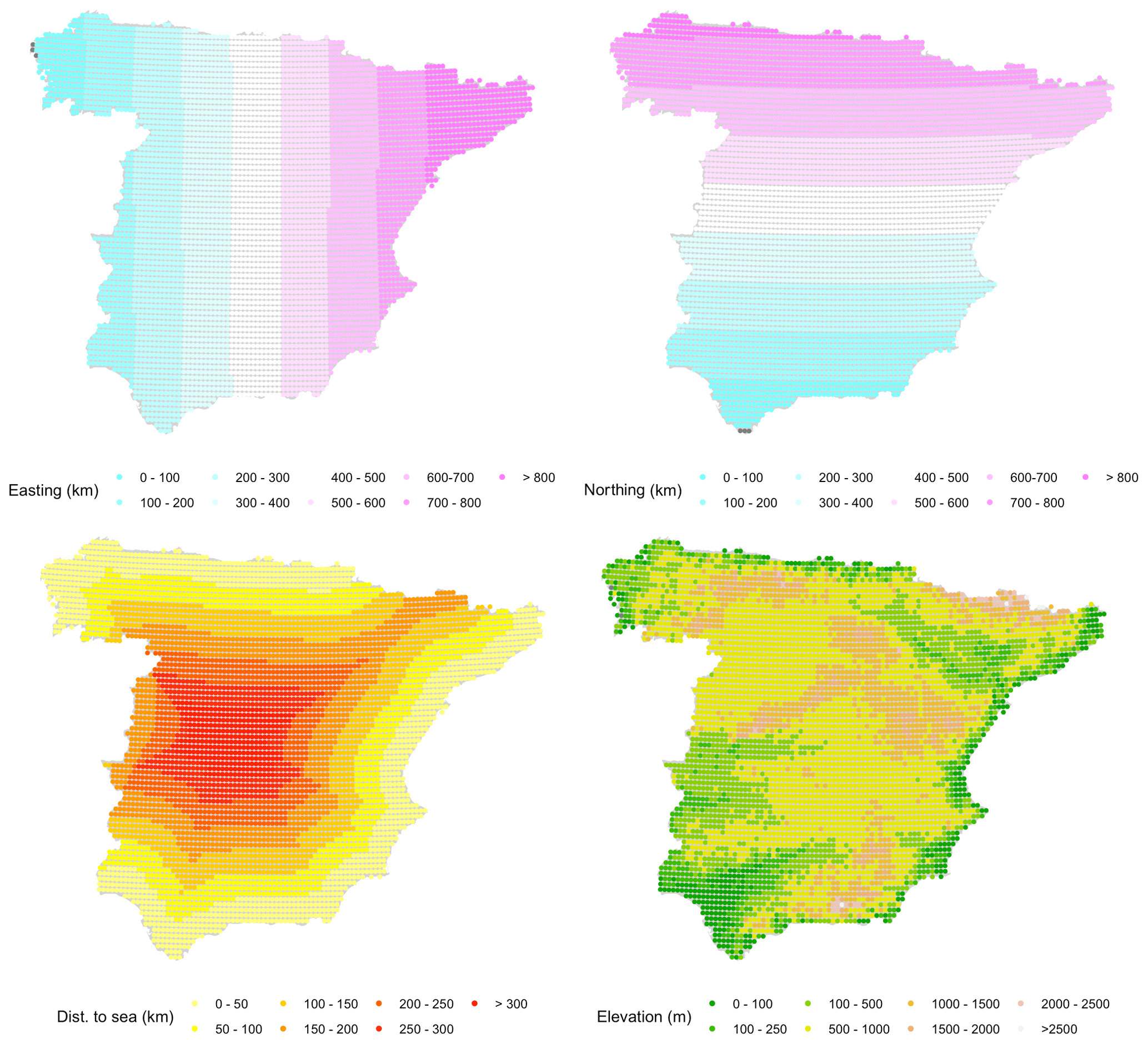
Figure A1 Fixed covariates used for universal kriging interpolation: easting and northing coordinates, elevation, and distance to the coastline.

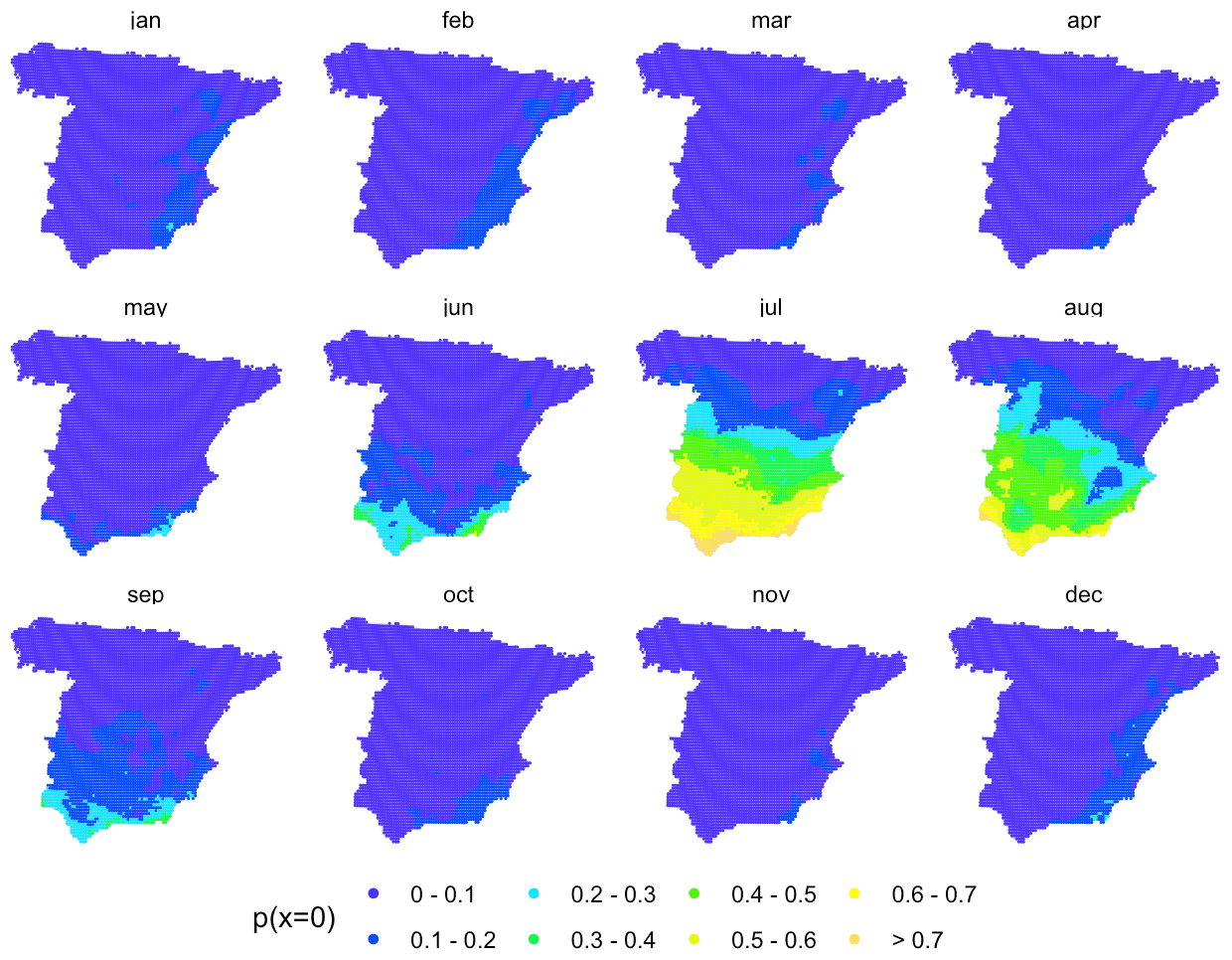
Figure A2 Mean monthly zero-precipitation probability over 1961–2000.

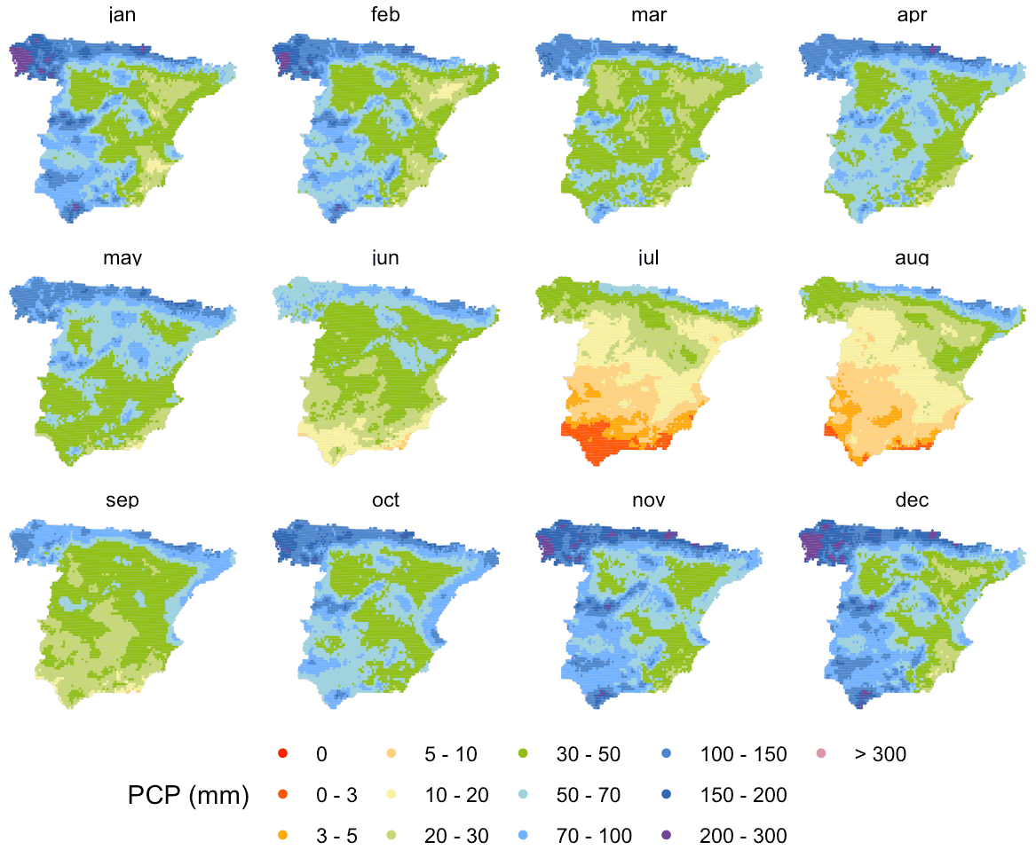
Figure A3 Mean monthly precipitation over 1961–2000.

Figure A4 Time evolution of the frequency of observations according to altitudinal classes.

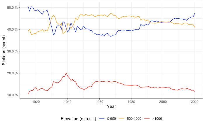
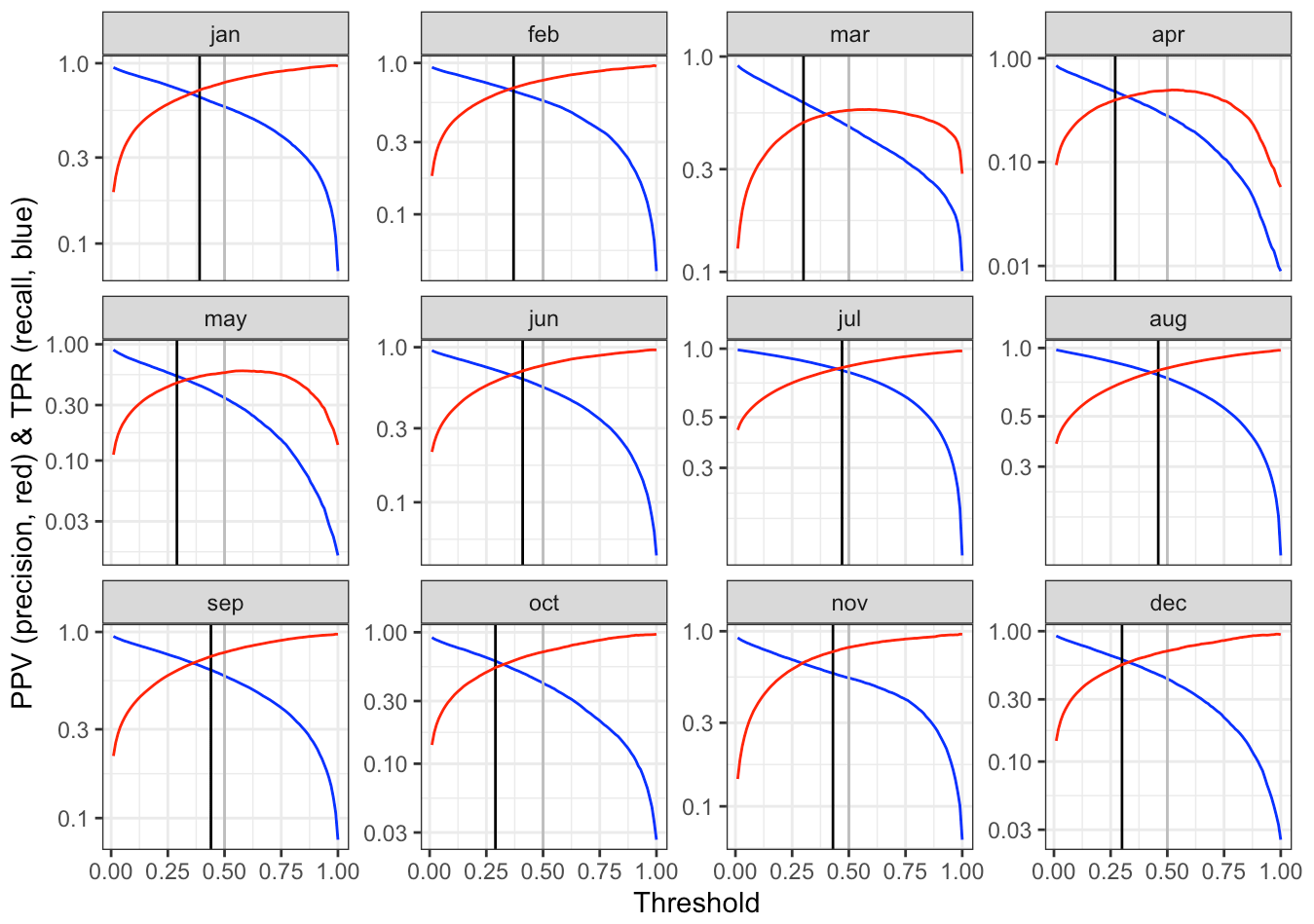
Figure A5 Positive prediction value and true positive rate vs. classification threshold obtained by cross-validation. The selected threshold is shown by vertical black lines.

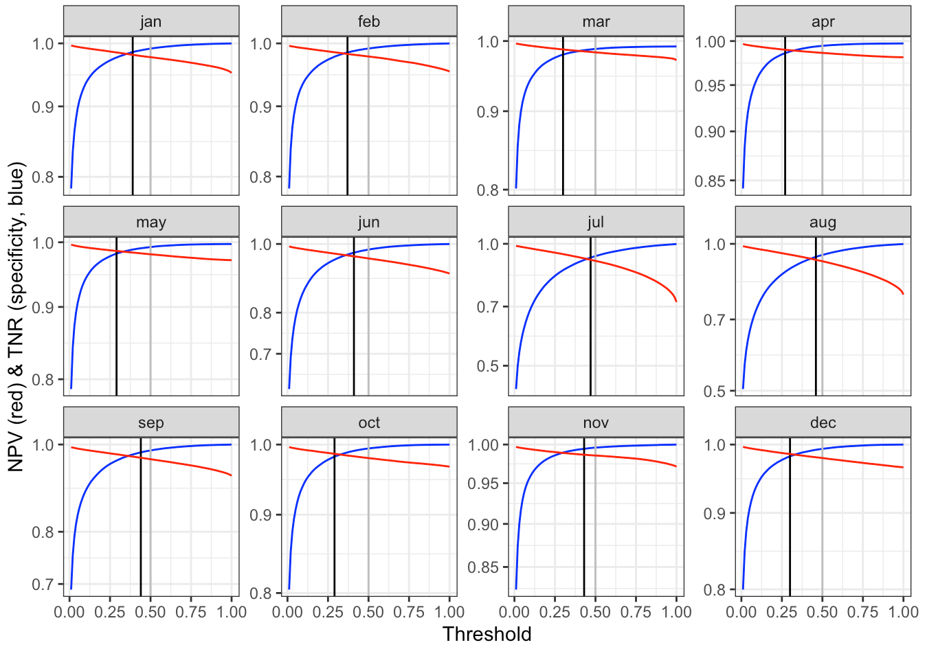
Figure A6 Negative prediction value and true negative rate vs. classification threshold obtained by cross-validation. The selected threshold is shown by vertical black lines.

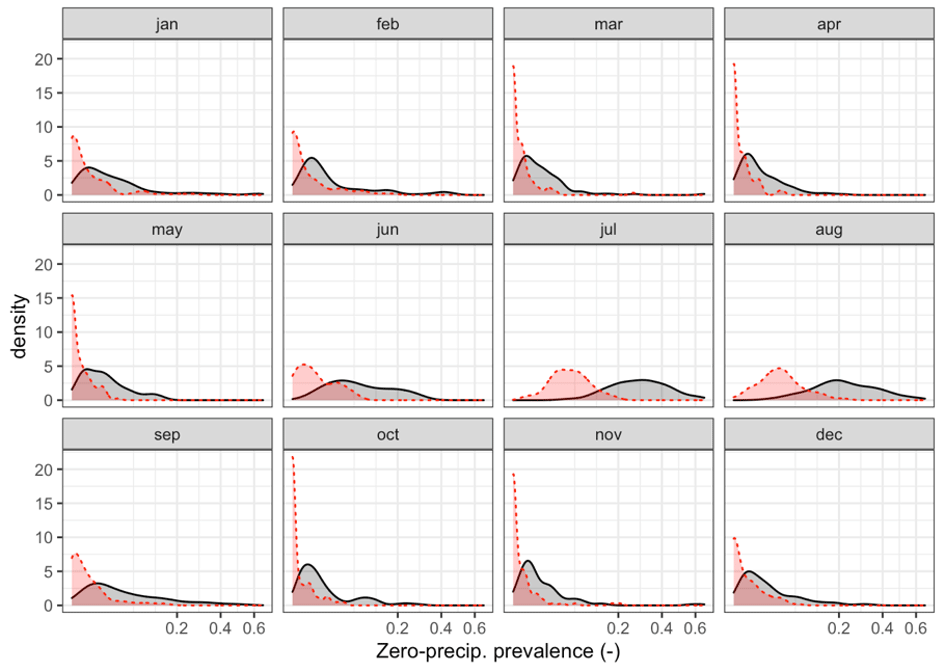
Figure A7 Empirical density functions of zero-precipitation frequency in the observed (grey) and cross-validation (red) datasets, using a single-step approach.

Figure A8 Time series of cross-validation mean error, performing a full standardization of the variable.

Table A1 Semivariogram models used in the interpolation of zero-precipitation probability and precipitation magnitude: exponential (Exp), Gaussian (Gau), spherical (Sph) and Matérn (Mat). Number of months.

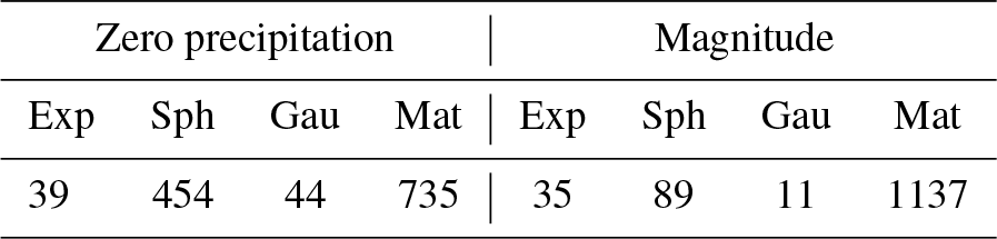
Table A2 Cross-validation statistics for zero precipitation and precipitation magnitude, using a single-step approach.

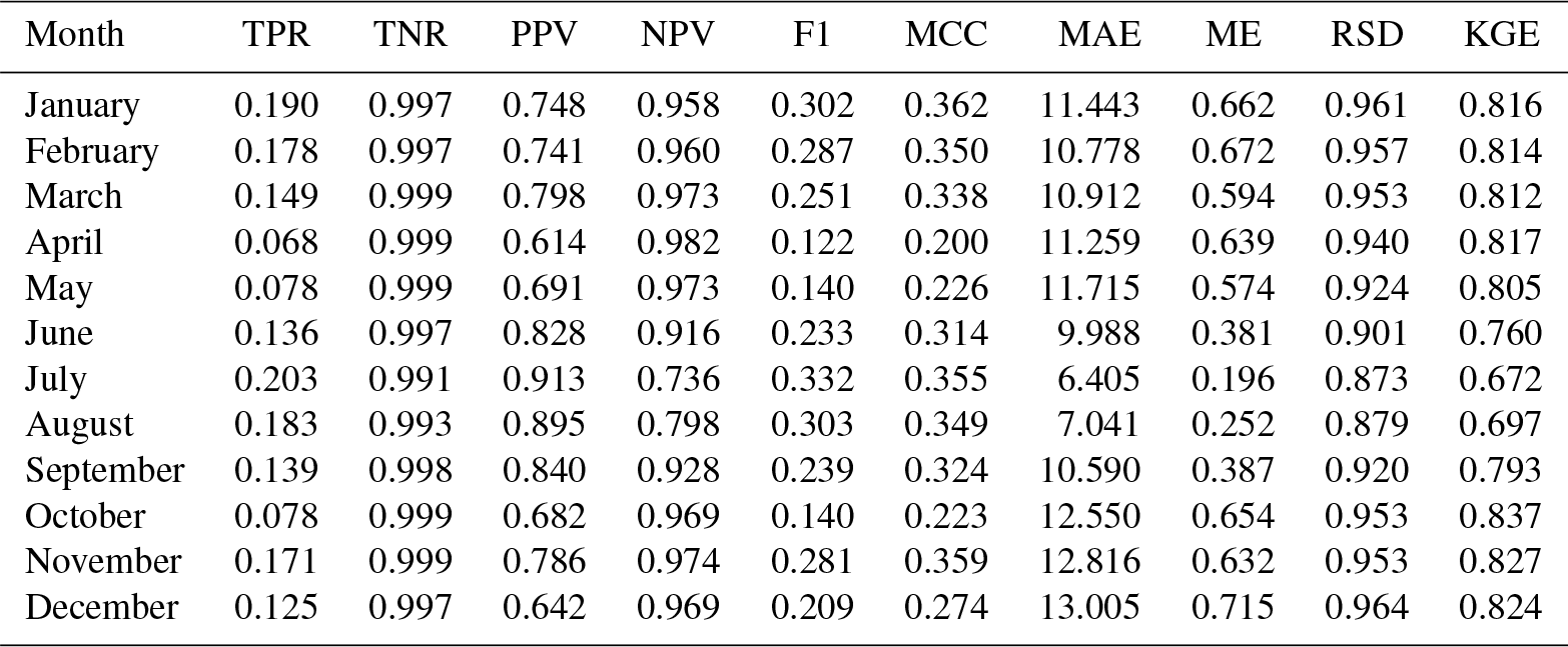
Table A3 Cross-validation statistics for precipitation magnitude, without variable transformation.

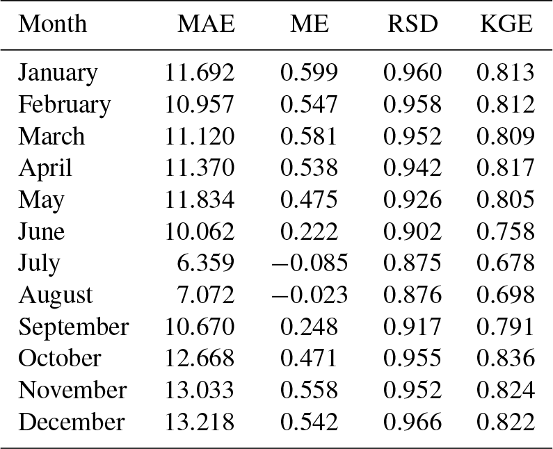
Table A4 Cross-validation statistics for precipitation magnitude, performing a full standardization of the variable.

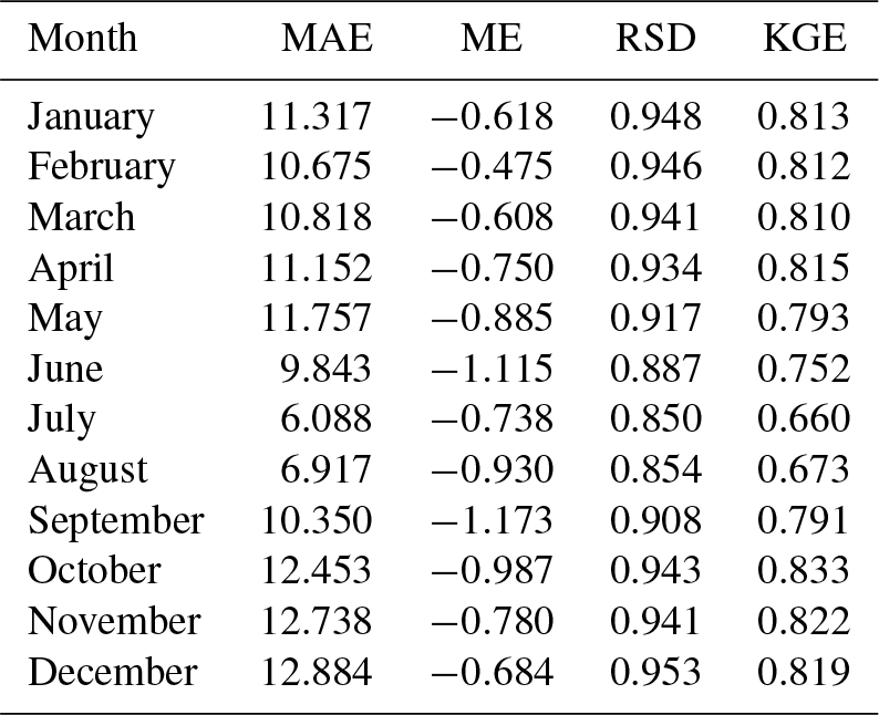
Table A5 Cross-validation statistics for zero precipitation and precipitation magnitude, using interpolation with no covariates (ordinary kriging). Median values across all the stations.

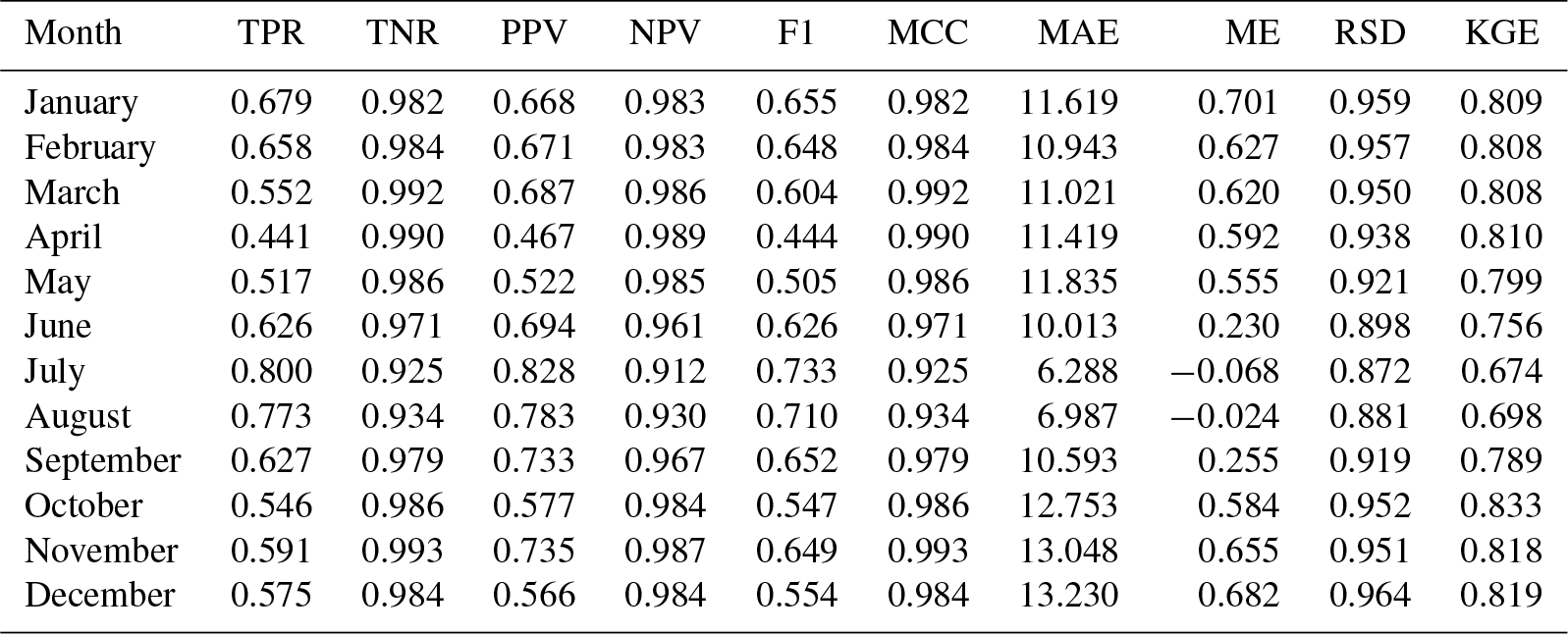
Table A6 Cross-validation statistics for precipitation magnitude, using a logarithmic variable transformation.

Table A7 Cross-validation statistics for precipitation magnitude, without the small offset.