Digital soil mapping of lithium in Australia

With a higher demand for lithium (Li), a better understanding of its concentration and spatial distribution is important to delineate potential anomalous areas. This study uses a digital soil mapping framework to combine data from recent geochemical surveys and environmental covariates that affect soil formation to predict and map aqua-regia-extractable Li content across the 7.6×10⁶ km² area of Australia. Catchment outlet sediment samples (i.e. soils formed on alluvial parent material) were collected by the National Geochemical Survey of Australia at 1315 sites, with both top (0–10 cm depth) and bottom (on average ∼60–80 cm depth) catchment outlet sediments sampled. We developed 50 bootstrap models using a cubist regression tree algorithm for each depth. The spatial prediction models were validated on an independent Northern Australia Geochemical Survey dataset, showing a good prediction with a root mean square error of 3.32 mg kg⁻¹ (which is 44.2 % of the interquartile range) for the top depth. The model for the bottom depth has yet to be validated. The variables of importance for the models indicated that the first three Landsat 30+ Barest Earth bands (red, green, blue) and gamma radiometric dose have a strong impact on the development of regression-based Li prediction. The bootstrapped models were then used to generate digital soil Li prediction maps for both depths, which could identify and delineate areas with anomalously high Li concentrations in the regolith. The predicted maps show high Li concentration around existing mines and other potentially anomalous Li areas that have yet to be verified. The same mapping principles can potentially be applied to other elements. The Li geochemical data for calibration and validation are available from de Caritat and Cooper (2011b; https://doi.org/10.11636/Record.2011.020) and Main et al. (2019; https://doi.org/10.11636/Record.2019.002), respectively. The covariate data used for this study were sourced from the Terrestrial Ecosystem Research Network (TERN) infrastructure, which is enabled by the Australian Government's National Collaborative Research Infrastructure Strategy (NCRIS; https://esoil.io/TERNLandscapes/Public/Products/TERN/Covariates/Mosaics/90m/, last access: 6 December 2022; TERN, 2019). The final predictive map is available at https://doi.org/10.5281/zenodo.7895482 (Ng et al., 2023).

1 Introduction

Minerals have become essential commodities in modern human society. Many minerals are fundamental to technological and industrial advancement, particularly those utilised in renewable energy systems, electric vehicles, consumer electronics, and telecommunications (Kabata-Pendias, 2010). These minerals can be considered critical in the sense that they are of high importance and have a high risk of supply disruption. Methods for quantifying mineral criticality are discussed in detail in Graedel et al. (2012).

Lithium (Li) is an important chemical element as the world transitions towards a lower-carbon economy. It has been listed as a critical element by various countries, including Australia, Canada, the European Union, Japan, the Republic of Korea, and the United States of America (Mudd et al., 2018; David Huston, Geoscience Australia, personal communication, March 2022). Australia is endowed with significant resources of many of the critical elements and the critical minerals hosting them, including Li. Currently, Australia's ranking for economic resources of Li is second, but it ranks first for its production (Senior et al., 2022), with potential for additional discoveries. According to a recent survey (Senior et al., 2022), Australia produced 40 kt (kilotons) of Li (in terms of spodumene, LiAlSi₂O₆, concentrates; assuming 6 % of Li₂O in spodumene concentrates) in 2020, or 49 % of the global production; a significant increase from 21.3 kt of Li in 2017 (Champion, 2019).

The two primary sources for Li are brine stores and mineral deposits, where Li is hosted mainly in spodumene. A 2013 investigation by Geoscience Australia found that the potential of Li-rich salt lakes in Australia was relatively low in comparison to those, for instance, in the Americas (Jaireth et al., 2013; Mernagh et al., 2013, 2016). Most of the Li in Australia exists as mineral deposits (Champion, 2019). Despite Australia's current position as the world's leading supplier of Li, it has limited prospects for immediate expansion as the potential for similar deposits in Australia has not yet been fully investigated (Mudd et al., 2018). This study aims to contribute to filling this knowledge gap by providing the first digital map of Li concentration in Australian soils.

Lithium values range from <1–15 mg kg⁻¹ in ultramafic rocks and 5.5–17 mg kg⁻¹ in mafic rocks, whereas felsic rocks (granite, rhyolite, and phonolite) contain higher Li concentrations, between 30–70 mg kg⁻¹ (de Vos et al., 2006). Lithium concentration in clay minerals ranges between 7–6000 mg kg⁻¹ (Starkey, 1982). With developments in technology, a process of extracting Li as Li-carbonate from certain minerals, other than spodumene, such as lepidolite (KLi₂Al(Si₄O₁₀)(F,OH)₂) and petalite (LiAlSi₄O₁₀), has been identified (Sitando and Crouse, 2012; Vieceli et al., 2018). Lower Li concentration is found in salt lake brine (0.17–1.5 mg kg⁻¹) (Grosjean et al., 2012). Extraction of Li from salt lake brine is in the form of Li-chloride, which needs to undergo an energy-intensive process to be converted to Li-carbonate from the Li metal forms for use in batteries.

Lithium is found in trace amounts in all soil types, primarily in the clay fraction, with slightly lower concentrations in the organic soil fraction (Kabata-Pendias, 2010). Possible means by which Li is bound to clay have been reviewed elsewhere (Starkey, 1982). Across Europe, values of Li ranging from 0.28–271 mg kg⁻¹ have been reported (Salminen et al., 2006), with smaller concentration ranges in agricultural soil (0.161–136 mg kg⁻¹) and grazing soil (0.1–153 mg kg⁻¹) (Reimann et al., 2014). Négrel et al. (2019) reported an aqua-regia-soluble Li concentration of 11.3 mg kg⁻¹ in European agricultural soil. In New Zealand, a study of Li concentration in soil reported a range between 0.08–92 mg kg⁻¹ (Robinson et al., 2018). de Caritat and Reimann (2012) reported median Li concentrations (after aqua regia digestion) of 12 and 5.7 mg kg⁻¹ in European agricultural topsoils and Australian surface sediments, respectively, both in the coarse (<2 mm) fraction. Subsequently, Reimann and de Caritat (2017) published the first continental map (Supplement; Fig. 2SM) of Li in Australian soils, based on National Geochemical Survey of Australia (NGSA) data, showing that regions of high and low concentrations are found across all Australian states. The amount of soil-available Li has been found to be relatively low, about 3 %–5 % of the total Li content in the surface layers both in the southeastern USA (Anderson et al., 1988) and Siberia (Gopp et al., 2018), ranging from 0.24–0.68 mg kg⁻¹. A total Li concentration within a range of 5.27–400 mg kg⁻¹ had been reported for catchment sediment samples in China (Liu et al., 2020) and within a range of <1–300 mg kg⁻¹ in the US topsoils (Smith et al., 2019).

Higher concentrations of Li are often found in the deeper layers of soil profiles (Merian and Clarkson, 1991). Typically, Li enters the soil profile through the weathering of sedimentary minerals in the underlying saprolite and bedrock (Aral and Vecchio-Sadus, 2008). Because clay minerals predominantly drive the mineralisation and dissolution of Li, the clay fraction will play a significant role in determining the Li concentration. The Li content of soil is controlled more by the soil formation conditions than by the composition of the parent materials (Kabata-Pendias, 2010). Similar observations are found in Négrel et al. (2019), where the aqua-regia-extractable Li concentrations can be linked with known mineralisation processes observed within Europe. This was also shown in the study by Luecke (1984), who explored the use of information on enriched elements (Rb, Ba, Sr, Cu, and Zn among others) to aid in predicting the distribution of Li pegmatites.

Mineral exploration aims to find ore deposits for mining purposes. Therefore, delineating target areas for mineral exploration through a series of mapping activities is a crucial initial stage leading to discovery (Carranza, 2011). Mineral prospectivity mapping (or modelling; MPM) is a method to quantify the probability of mineralisation in a selected area for mineral exploration purposes (Zuo, 2020). This prioritisation allows for the selection of smaller, higher-potential areas for detailed prospecting investment to minimise exploration costs, e.g. the number of drillholes.

Two common paradigms for creating MPM are knowledge-driven and data-driven models (Carranza, 2011). Knowledge-driven models do not require any data on mineral deposits but rely on expert knowledge of spatial associations between mineral deposits and geological features, field experience, and conceptual models to develop evidential maps that enable the discovery of mineral deposits (Carranza, 2008). Conversely, data-driven models utilise existing knowledge on the location of mineral occurrences, various survey datasets, and spatial statistical methods to represent the likelihood of mineral occurrence within prospective areas (Carranza, 2008). Numerous data-driven models have been derived for the detection of anomalous mineral occurrences. Benedikt (2018) utilised Tellus regional stream sediment geochemistry to screen for anomalous metal abundances within minerals in southeast Ireland. Roshanravan et al. (2023) and Harris et al. (2023) also implemented a data-driven machine learning model to develop predictive maps of gold prospects.

With the development of machine learning and technology (computer hardware, software, and geographic information system (GIS) technology), there have been growing applications of MPM in recent decades (Carranza, 2011; Porwal et al., 2015; Zuo, 2020). Several studies have demonstrated the use of remote sensing to explore various deposit types, such as gold (Au) deposits (Crósta et al., 2010), copper (Cu) deposits (Pour and Hashim, 2015), and iron (Fe) ores (Ducart et al., 2016). The application of remote sensing for Li deposits has also emerged. Gopp et al. (2018) explored the use of a normalised difference vegetation index (NDVI) to develop a predicted map of the plant available content of Li in southwestern Siberian soil. Cardoso-Fernandes et al. (2018, 2020) evaluated the potential use of Sentinel-2 in Li mapping in the Fregeneda–Almendra region across the Spain–Portugal border. Similarly, Köhler et al. (2021) further explored the use of combined geological data and Sentinel-2 data for Li potential mapping in Portugal. Antezana Lopez et al. (2023) used Sentinel-2, ASTER, Jilin GP, and PROBA CHRIS satellite data to study surface reflectance, as well as soil physicochemical properties, to predict Li concentration in Bolivian salt flats.

In soil science, digital soil mapping (DSM) has been widely used to produce quantitative maps of soil attributes based on the known distributions of environmental covariates (i.e. rainfall, parent material, vegetation, and landforms) that affect soil formation. The DSM framework is derived from the conceptual model developed by McBratney et al. (2003) in which a certain soil attribute results from the interaction of soil-forming factors. These factors are modified from Jenny (1941) and include soil (s), climate (c), organisms (o), relief (r), parent material (p), age/time (a), and spatial position (n), or “scorpan”. The factors are measured or approximated from various data types, including point observations, maps (polygons), survey data, and remote sensing data, as well as derivatives thereof (e.g. gradients, buffer distances); these can be numerical or categorical data types.

In this study, we attempt to model Li distribution in the surface and subsurface soils of Australia by invoking the NGSA soil geochemistry dataset and various environmental covariates commonly used in DSM related to soil formation in Australia. In detail, the objectives of this study are thus to

1. evaluate the use of a DSM framework to predict Li concentrations in Australian soils and

2. delineate anomalous areas potentially attractive for Li exploration and discuss their interpretations.

2 Materials and methods

2.1 Li measurement

This study used two soil datasets, referred to as the calibration and validation datasets. The calibration dataset was used to build the spatial prediction model, and the validation dataset was used to test the prediction quality of the calibrated model.

The calibration dataset data were generated as part of the NGSA project (https://www.ga.gov.au/about/projects/resources/national-geochemical-survey, last access: 5 May 2023), a collaborative project between Geoscience Australia and the Australian states and Northern Territory between 2007–2011, which aimed to document the soil geochemical concentration levels and patterns across Australia. Details on the project, analysis, sampling methods, and the measurement of other parameters can be found in de Caritat and Cooper (2011b, 2015) and de Caritat (2022).

The NGSA collected samples at 1315 sites (including field duplicates) at or near the outlet of large catchments with a total area coverage of 6.17×10⁶ km² and an average sampling density of one site for every 5200 km² (de Caritat and Cooper, 2011b). The target sampling medium was floodplain sediments away from river channels, though in various places in Australia, aeolian modification of floodplain sediments can be important; thus, the medium was called “catchment outlet sediment” rather than floodplain sediment. These geomorphological entities are typically vegetated and biologically active (plants, worms, ants, etc.), thereby making the collected materials true soils (e.g. SSSA, 2022), albeit soils all developed on transported alluvium parent material. Due to limitations to access, samples from some parts of South Australia and Western Australia could not be obtained.

Samples were collected from two depths, namely “top outlet sediment” (TOS) from 0–10 cm depth, and “bottom outlet sediment” (BOS) from, on average, ∼60–80 cm depth. All of the samples were air-dried, homogenised, and dry sieved to <2 mm and <75 µm prior to various analyses for 60 plus elements (see de Caritat et al., 2009, 2010, for a full description of the NGSA sample preparation and analytical methods, respectively).

In this contribution, we use Li concentrations after aqua regia digestion, as the NGSA did not report total Li. A 0.50 ± 0.02 g aliquot of sample (<2 mm) was digested in aqua regia (1.8 mL of HCl + 0.6 mL of HNO₃) at 90 ± 3 ^∘C for 2 h to leach acid-soluble components. Once the sample had cooled to room temperature, 17.5 mL of diluent was added, and the sample was inverted 10 times to homogenise the content. The sample was further diluted 50 times prior to analysis, using inductively coupled plasma mass spectrometry (ICP-MS) in a commercial laboratory (de Caritat et al., 2010). For the remainder of the paper, any reference to Li concentrations is understood to mean aqua-regia-extractable Li unless otherwise noted. Any Li measurements that fell below the detection limit (0.1 mg kg⁻¹) were replaced with half the detection limit (0.05 mg kg⁻¹). A detailed quality assessment of the NGSA data is given in de Caritat and Cooper (2011a), where a relative analytical precision (repeat analysis of TILL-1 Certified Reference Materials (CRM)) of 12 % and a relative overall precision (based on field duplicates) of 39 % were reported. The distribution of sampling sites and Li concentration levels for both TOS and BOS are shown in Fig. 1.

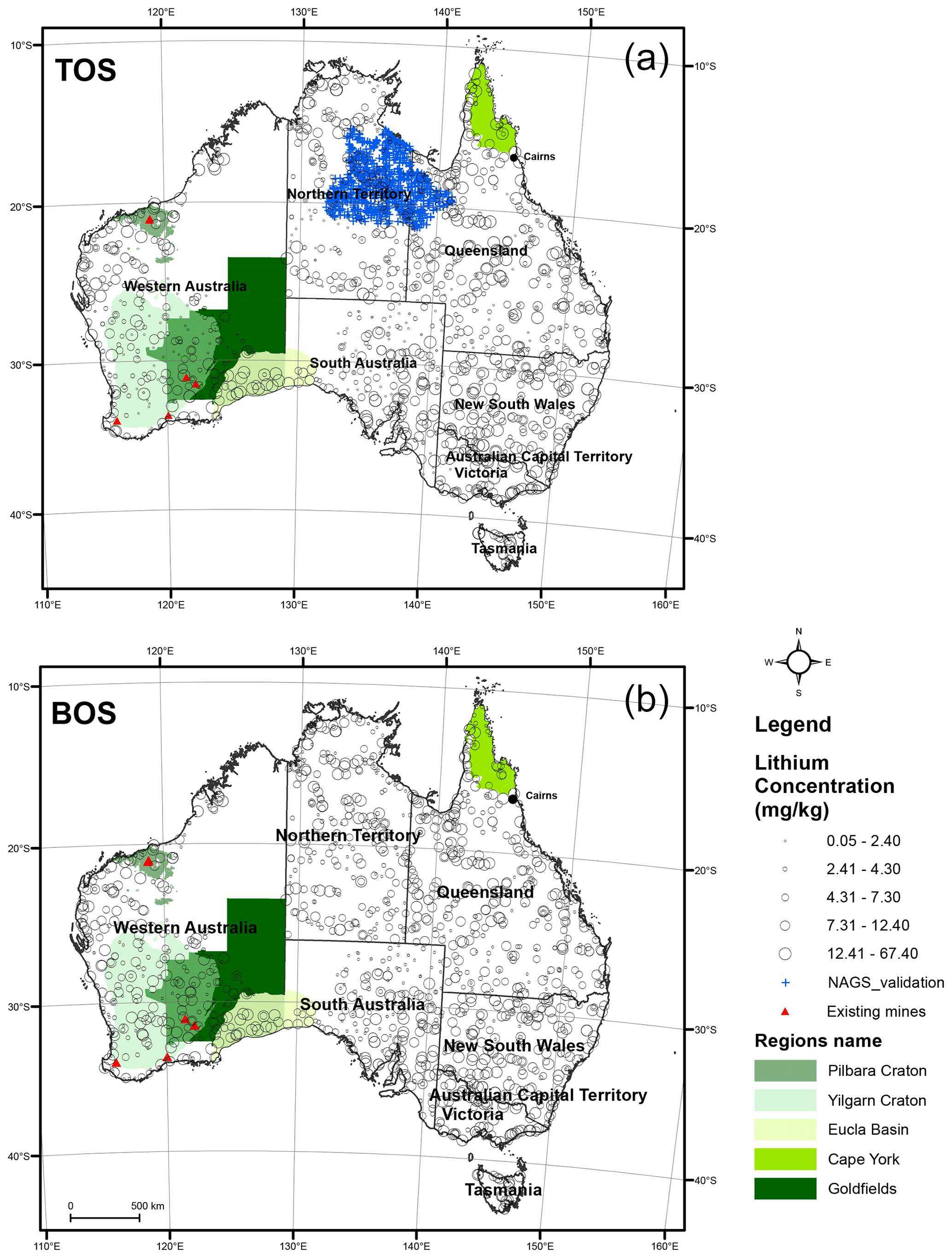
Figure 1 Distribution of sampling sites from the National Geochemical Survey of Australia (NGSA, black circles) for both depths: top outlet sediment (TOS) 0–10 cm (a) and bottom outlet sediment (BOS) ∼60–80 cm (b). Distribution of sampling sites from the Northern Australia Geochemical Survey (NAGS, blue plus signs) for TOS only (a). All data refer to the coarse fractions (<2 mm). Aqua-regia-soluble Li concentrations (mg kg⁻¹) are categorised in five quantile classes. Regions discussed in the text are highlighted in various shades of green. Projection: Australian Albers equal area (EPSG:3577). Data sources: de Caritat and Cooper (2011b), Hughes (2020), and Main et al. (2019).

As an independent validation dataset, we used the geochemical dataset from the Northern Australia Geochemical Survey (NAGS) project (Main et al., 2019). This dataset contains 773 observations located in the Tennant Creek–Mount Isa region in the Northern Territory and Queensland, with an approximate sampling density of one sample every 500 km² and collection in 2017. The distribution of these samples is also shown in Fig. 1. These samples were collected, prepared, and analysed following the NGSA protocols (de Caritat and Cooper, 2011b), albeit at a higher sampling density. However, only TOS samples were collected in NAGS. Furthermore, these NAGS samples were collected at a different time and analysed in a different laboratory compared to the NGSA dataset. To address the analytical variation that could potentially arise, a levelling method was applied using the TILL-1 CRM standards (Main and Champion, 2022). First, the subset of the NGSA dataset that covers the spatial area of the NAGS dataset was extracted. Then a Kolmogorov–Smirnov test was used to verify if the samples from the two datasets (subset of the NGSA and NAGS) were similar. A correction factor to relate the two datasets based on the TILL-1 CRM standards was then calculated and applied as a multiplier to the NAGS dataset to level its data to the NGSA dataset.

2.2 Environmental covariates

A total of 19 environmental covariates (Table 1) characterising the factors of climate, parent material, soil, and topography, which contribute to soil formation, were considered in this study.

Table 1 Environmental covariates used for digital soil mapping of Li.

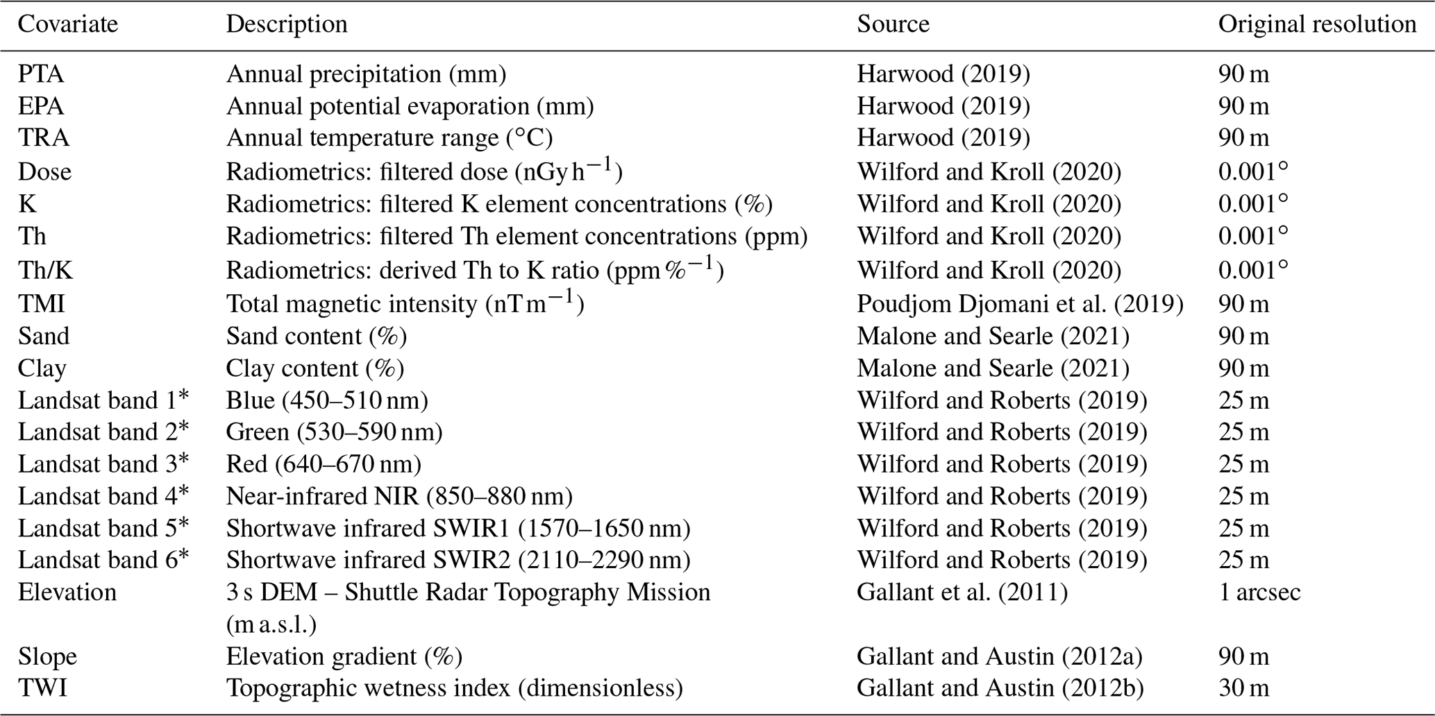
^∗ All Landsat bands referred to here are from the Landsat 30+ Barest Earth products.

The first factor is climate. Water (humidity) and temperature affect the rate of mineral weathering and thus soil formation. Hence, we included precipitation, evaporation, and temperature data (Harwood, 2019), along with the topographic wetness index (TWI) data (Gallant and Austin, 2012b), informing about the relative wetness within a landscape. In short, the TWI was derived from the partial contributing area product, which was computed from a hydrologically enforced digital elevation model, and from the percent slope product, which was computed from the smoothed digital elevation model (DEM-S; Gallant and Austin, 2012b).

The second factor is parent material (i.e. degree of weathering and mineralogical composition), including gamma-ray radiometric and total magnetic intensity. Gamma-ray radiometric surveys provide estimates for the concentrations of gamma-ray-emitting radio-elements like potassium (K), uranium (U), and thorium (Th) at/near the soil surface. The gamma-ray radiometric data were measured from airborne surveys throughout most of Australia (Poudjom Djomani et al., 2019). In this study, we used a complete gamma-ray survey grid where gaps in the airborne coverage were filled in using covariate machine learning (Wilford and Kroll, 2020). Gamma-ray radiometric data have been found to be a useful covariate in identifying surface processes such as sediment transport and weathering (Wilford, 2012; Wilford et al., 1997) and detecting radioactive mineral deposits and occurrences (Alhumimidi et al., 2021; Dickson et al., 1996; Dickson and Scott, 1997; Wilford et al., 2009). Total magnetic intensity (TMI), which measures variations in the Earth's magnetic field intensity caused by the contrasting content of various rock-forming minerals in the crust (Poudjom Djomani et al., 2019), could also potentially identify geological features and processes.

The third factor is the soil itself, particularly the relevant physical soil properties. As previous studies, e.g. by Kabata-Pendias (1995) and Robinson et al. (2018), highlighted the high correlation between Li and clay content of soil, soil texture was used as a covariate. The soil texture spatial information (sand and clay contents) was derived from Malone and Searle (2021), which contained updated information on soil texture across Australia derived using a digital soil mapping approach. The sand and clay fractions were developed by integrating field morphological (n=180 498) and laboratory measurements of soil texture fractions (n=17 367) from the Soil and Landscape Grid of Australia (SLGA). The SLGA is based on a comprehensive compilation of soil attributes across Australia, including the NGSA dataset. These sand and clay content maps (Malone and Searle, 2021) were for specific depth intervals (0–5, 5–15, 15–30, 30–60, 60–100, and 100–200 cm). They were converted to the depths corresponding to the NGSA Li measurement (0–10 and ∼60–80 cm) using the mass-preserving spline function, described in Bishop et al. (1999) and modified by Malone et al. (2009). Soil reflectance in the visible, near-infrared (NIR), and shortwave–infrared (SWIR) spectra captured by remote sensing images provides information on soil composition. However, the unprocessed images consist of a mixture of soil, bedrock, vegetation, and clouds. By removing the influence of seasonal vegetation, Roberts et al. (2019) were able to document the “barest” state of soil, so critical in mapping the physical characteristics of soil and rock. This was done by combining Landsat 5, 7, and 8 observations of the past 30 years to remove the contamination by seasonal vegetation, cloud cover, shadows, detector saturation and pixel saturation. The model used to develop the Barest Earth product was validated using the NGSA spectral archive (Lau et al., 2016).

Finally, topography is represented by elevation and slope. These factors also play an important role, as they affect how water is added to and/or lost from soil. The elevation was derived from the DEM-S which was obtained from the 1 arcsec resolution Shuttle Radar Topography Mission (SRTM) data acquired by NASA in February 2000 (Gallant et al., 2011). The slope covariate was also calculated from DEM-S using the finite difference method (Wilson and Gallant, 2000). The different spacing in the E–W and N–S directions due to the geographic projection of the data was accounted for by using the actual spacing in metres of the grid points calculated from the latitude.

All covariates were reprojected to EPSG: 3577 (GDA94 datum; Australian Albers equal area projection) and resampled to a common spatial resolution of 3 km prior to any analysis. All the environmental covariates used are shown in Table 1.

The correlation matrix of the Li concentrations to all the other element concentrations and environmental covariates was generated using Pearson's correlation method. Strong correlation was defined as >0.5, moderate was defined as 0.35 to 0.5, and weak correlation was defined as <0.35. Note that this classification was generated to facilitate interpretation of this dataset only and is not implied to be a general rule.

2.3 Modelling

Here, we used the machine learning model “cubist” to relate soil observations to the environmental covariates. Cubist is a tree-based regression algorithm based on the M5 theory (Quinlan, 1993). This algorithm creates partitions of data with similar spectral characteristics and creates one or more rules for each partition. If the partition rules are satisfied, then the linear regression of that partition is used to create the prediction (Eq. 1). Each rule can be defined as follows:

$$\begin{array}{}\text{(1)}& \mathrm{\text{If [condition is true], then [regression], else [apply next rule]}}.\end{array}$$

The cubist model has two tuning parameters: committees (number of sequential models included in the ensemble) and neighbours (number of training instances that are used to adjust the model-based prediction). A comprehensive combination of committees (5, 10, 20, 30, 40, 50) and neighbours (0, 1, 5, 9) was tested to tune the cubist model. To obtain the best estimates of optimum parameters, a 10-fold cross-validation approach was utilised. Based on the optimum parameters, 50 bootstrap models (“sampling with replacement”) were trained. The flowchart of the process is shown in Fig. 2.

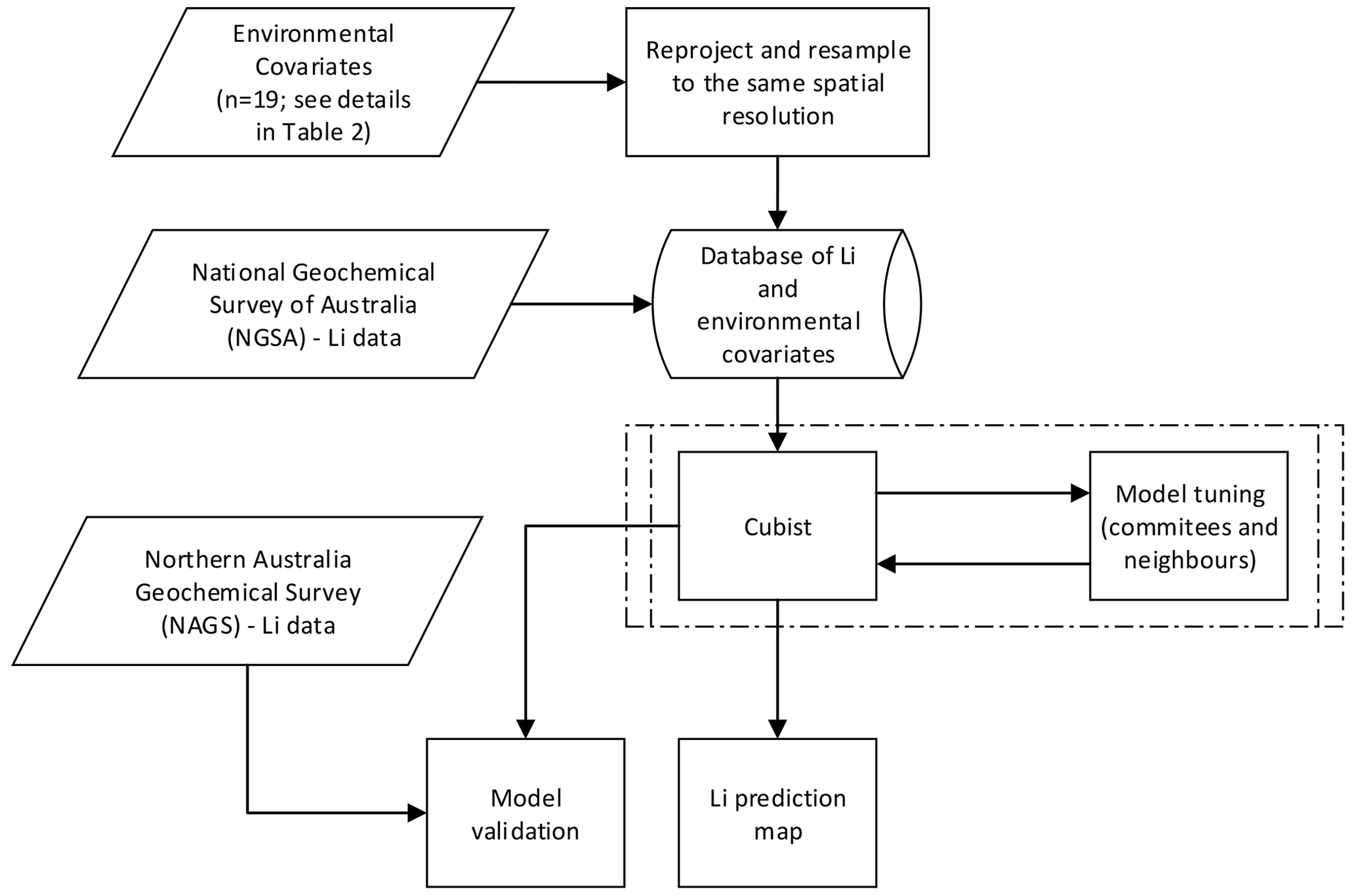
Figure 2 Flowchart of cubist model training to generate Li prediction map along with model validation.

The performance of the prediction models was then evaluated using both an internal evaluation and the external, independent validation dataset. An internal evaluation of the model was conducted using “out of bag” samples, which were not used during the development of the bootstrap models. The NAGS dataset was used to evaluate the performance on the independent dataset (top depth only). The following metrics, briefly explained below, were used: adjusted coefficient of determination ($R_{\text{adj}}^{\mathrm{2}}$), Lin's concordance correlation coefficient (LCCC) (Lin, 1989), root mean square error (RMSE), bias, and ratio of performance to interquartile distance (RPIQ). $R_{\text{adj}}^{\mathrm{2}}$ is a measure of the linear association between observed and predicted values; LCCC measures the agreement between the observed and predicted values in relation to the 1:1 line while accounting for the magnitude of the differences; RMSE is a measure of the differences between the observed and predicted values; bias is the measure of the difference between the mean of the observed and the mean of the predicted values; and RPIQ is a measure of performance that takes into account the distribution of the values and can be calculated as a fraction of the interquartile range of the observed values (Q₃−Q₁) and the RMSE ($\text{RPIQ}=(Q_{\mathrm{3}}-Q_{\mathrm{1}})/\text{RMSE}$) (Bellon-Maurel et al., 2010).

Variable importance analysis was also conducted to evaluate the contributions of each covariate to the Li prediction. The relative variable importance is measured as the percentage of times the environmental covariate is used either as conditions for a rule or as predictors (usages) within the linear regression model when certain conditions are met. These bootstrap models were then used to generate output maps with the same extent and resolution. The final map output was derived based on the mean prediction of the bootstrap models; similarly, the standard deviation map was obtained based on the standard deviation of the prediction from the bootstrap models.

2.4 Data processing and statistical computing

All the data analytics, modelling, and mapping procedures in this study were conducted in the R statistical open-source software (R Core Team, 2021). Besides the base R functionality, the R packages used in this study included “cubist” (Kuhn and Quinlan, 2021) for fitting cubist models, “caret” (Kuhn, 2022) for tuning the hyperparameter of the cubist model, and “raster” (Hijmans, 2021) for handling raster layers and generating soil map predictions. All soil maps were produced in ArcMap version 10.8 (ESRI, 2019) using the Albers equal area projection (EPSG:3577).

3 Results and discussion

3.1 Descriptive analysis

The distribution of 1315 aqua-regia-soluble Li concentration values (NGSA dataset; de Caritat and Cooper, 2011b) was positively skewed (Fig. 3) with concentrations ranging from 0.05–67.4 and 0.05–56 mg kg⁻¹ for TOS and BOS, respectively. Only limited observations above 20 mg kg⁻¹ of Li concentrations were found in this study for both TOS (n=76) and BOS (n=95). The mean concentration of TOS (7.6 mg kg⁻¹) was slightly lower than that of BOS (8.8 mg kg⁻¹). These concentrations were lower than those observed for the mean aqua-regia-soluble Li concentrations in European soil at 11.3 mg kg⁻¹ (Négrel et al., 2019), as well as those found in upper continental crust (both in loess and shales) at 35 mg kg⁻¹ total Li (Teng et al., 2004). A soil geochemical survey in the USA shows total soil Li concentrations with a range of <1–300 mg kg⁻¹ (median 20 mg kg⁻¹) for soils from 0–5 cm and a range of <1–280 mg kg⁻¹ (median 24 mg kg⁻¹) for soil samples from the C horizon (Smith et al., 2019). Similarly, total Li concentrations of up to 400 mg kg⁻¹ have been reported in China (Liu et al., 2020). These latter Li concentrations, measured using an extraction of four acids, were considerably higher than the aqua regia extraction data from the NGSA dataset.

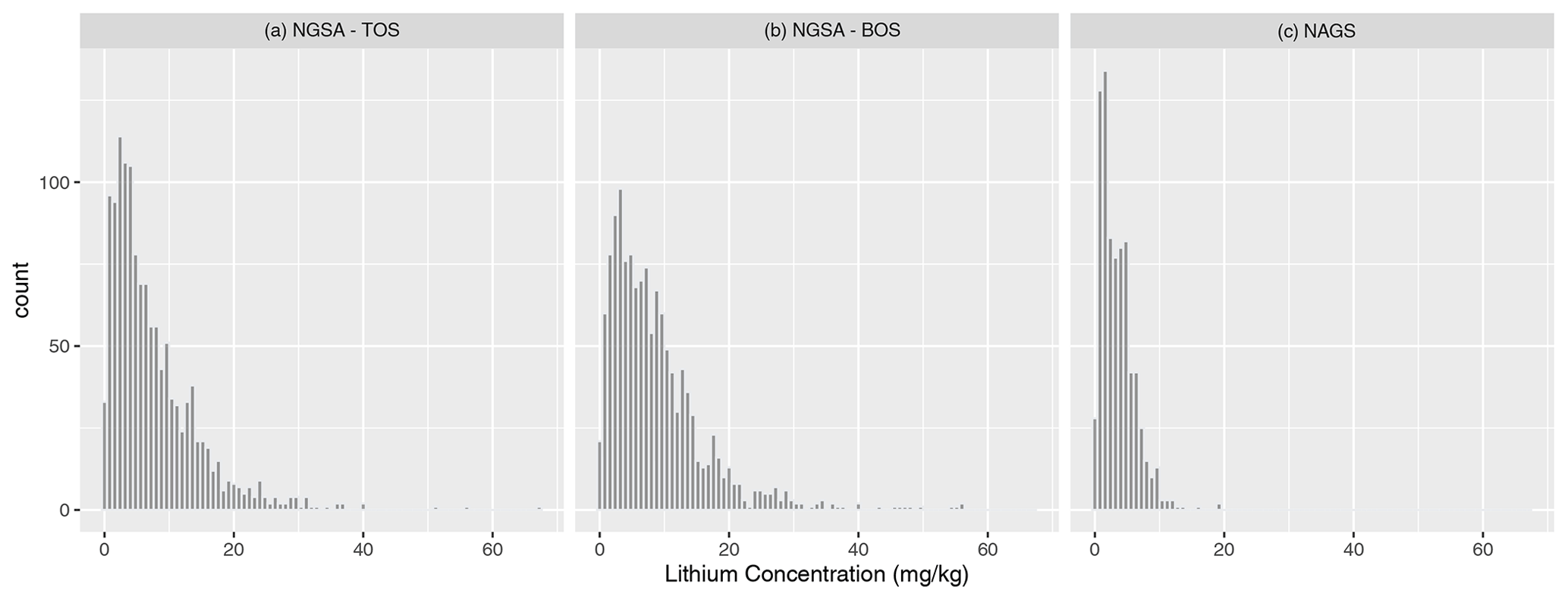
Figure 3 Histograms of Li concentrations for both NGSA depths: top outlet sediment (TOS) 0–10 cm (a), bottom outlet sediment (BOS) ∼60–80 cm (b), and NAGS (c). Data source: de Caritat and Cooper (2011b) and Main et al. (2019).

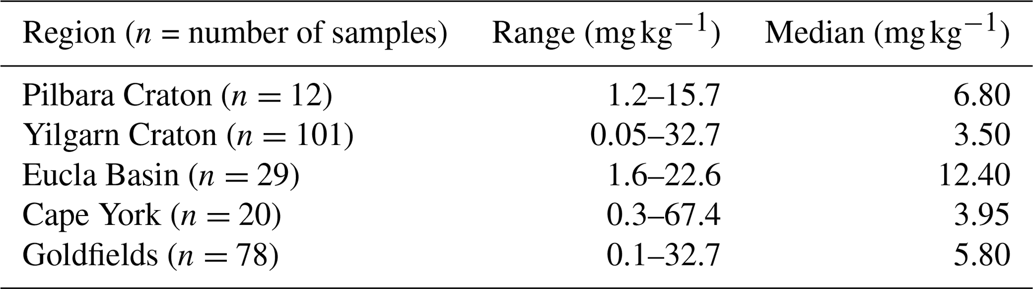
Based on the data collected by the NGSA project, the highest concentrations of Li for both TOS and BOS were found in northernmost Queensland (Cape York Peninsula), as shown in Fig. 1 and Table 2. Other regions that have elevated concentrations of Li were located in the Goldfields–Esperance region (Table 2) in Western Australia, which has been recognised as one of the most resource-rich areas on the planet (Champion, 2019), and the region around the Victoria–New South Wales border (Fig. 1). Some of the findings correlate well with the existing Li mine sites in Australia (red triangles in Fig. 1). The largest deposit of Li found in Australia is the Greenbushes deposit, south of Perth. Other regions include Mount Marion and Earl Grey in the Yilgarn Craton and Pilgangoora in the Pilbara Craton (Champion, 2019; see Table 1). In July 2019, Strategic Metals Australia (SMA) found a new Li exploration target near Cairns, in the Georgetown province of north Queensland (Gluyas, 2019). However, this discovery has not been updated in the data collected by Geoscience Australia because considerable work such as drilling, modelling, resource calculation, and feasibility studies are needed to bring the discovery to the feasibility stage.

Table 2 Aqua-regia-extractable lithium concentrations across various regions of Australia.

3.1.1 Correlation between Li with other measured properties

Despite other studies reporting strong correlations between Li and Mg (Kashin, 2019; Robinson et al., 2018) and between Li and other elements elsewhere, including Al, B, Fe, K, Mn, and Zn, the NGSA data only show strong correlations (as defined above) between Li and Al (Pearson's correlation coefficient r=0.74), Ga (r=0.69), Cs (r=0.68), and Rb (r=0.66) for TOS and slightly lower correlations for BOS: Al (r=0.69), Ga (r=0.64), Cs (r=0.62), and Rb (r=0.61). Correlations between Li and K and Mg were only moderate for both TOS (r=0.48 and 0.43) and BOS (r=0.46 and 0.33). de Vos et al. (2006) also observed good correlations (r>0.4) between total Li and Al, Ga, and Rb within the floodplain sediment samples. Similarly, Cardoso-Fernandes et al. (2022) found strong correlation between total Li and Sn, B, Rb, Cs, and F in stream sediment samples using geochemical pathfinder analysis. More details on the correlation between Li and other geochemical properties are included in Table S1 in the Supplement.

The Li concentration in soil was (strongly) negatively correlated with measured sand content from the NGSA dataset ($r=-\mathrm{0.55}$) and (moderately) positively correlated with clay content (r=0.44). This is consistent with the findings of Kabata-Pendias (2010) and Robinson et al. (2018), who noted the tendency of clay minerals to concentrate Li. It has been suggested that Li may be located internally within clay minerals – mainly kaolinite, illite, and smectites including hectorite, palygorskite, and sepiolites – in ditrigonal cavities via isomorphous substitution rather than on exchange sites (Anderson et al., 1988; Starkey, 1982) as a result of subsolidus cation exchange reactions with residual pegmatitic fluids (London and Burt, 1982).

3.1.2 Correlation with environmental covariates

Overall, the correlation between Li concentration and the environmental covariates was weak (Fig. 4). The correlation with sand and clay content derived from digital soil maps was lower in comparison to the measured (NGSA) values discussed above, with $r=-\mathrm{0.28}$ and 0.25, respectively, for TOS and $r=-\mathrm{0.23}$ and 0.22, respectively, for BOS.

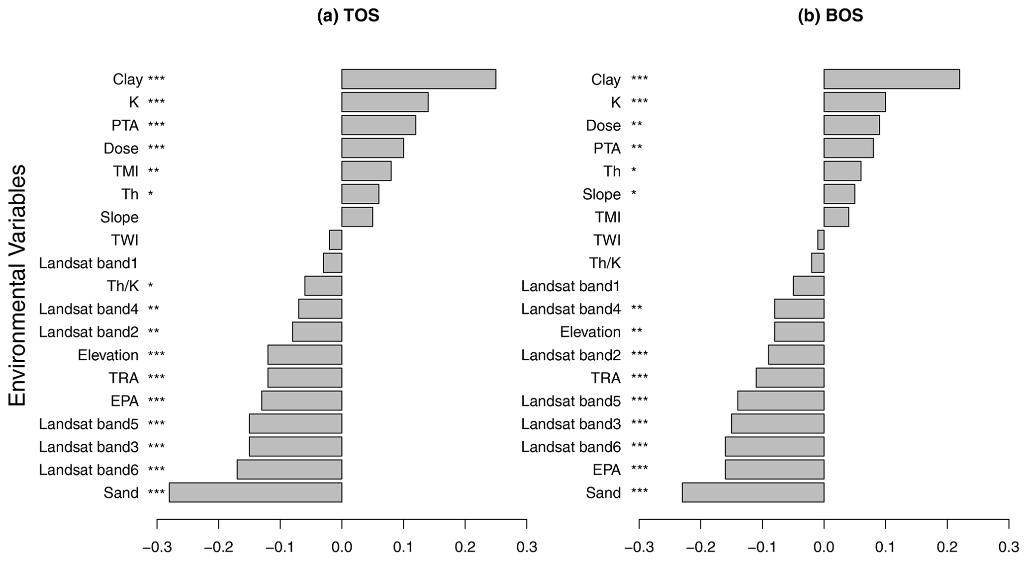
Figure 4 Pearson's correlation coefficient (r) between Li content and the environmental covariates (scorpan) for both NGSA depths: top outlet sediment (TOS) 0–10 cm (a) and bottom outlet sediment (BOS) ∼60–80 cm (b). Data sources: de Caritat and Cooper (2011b), Gallant et al. (2011), Gallant and Austin (2012a, b), Harwood (2019), Wilford and Roberts (2019), Poudjom Djomani et al.  (2019), Wilford and Kroll (2020), Malone and Searle (2021). See Table 1 for abbreviations. ${}^{\ast \ast \ast }$ Correlation is significant at the 0.001 level. ${}^{\ast \ast }$ Correlation is significant at the 0.05 level. ^∗ Correlation is significant at the 0.01 level.

For TOS, the Landsat bands 3 (red), 5 (SWIR1), and 6 (SWIR2) had similar (weak) negative correlations with Li content ($r=-\mathrm{0.15}$ to −0.17). For gamma-ray radiometric data, both total dose and K content had weak correlations with Li (r=0.10 to 0.14). These positive correlations are expected as the associations of Li deposits and felsic rocks (high in both total dose and K) due to the observed incompatibility in mineral structures (Benson et al., 2017). Precipitation had a weak positive correlation (r=0.12), while both temperature and elevation had weak negative correlations ($r=-\mathrm{0.12}$) with Li content. TWI and slope had negligible correlation with Li content ($r=-\mathrm{0.02}$ to 0.05).

For BOS, similar observations on the correlations between Li content and environmental covariates were found where temperature and Landsat bands 3, 5, and 6 had (weak) negative correlations ($r=-\mathrm{0.11}$ to −0.16) with Li, while radiometric K (r=0.10) and dose (r=0.09) had (weak) positive correlation with Li. Similarly, TWI and slope showed negligible correlation with Li ($r=-\mathrm{0.01}$ to 0.05).

3.2 Model evaluation

The final cubist model was tuned with 20 committees and 9 neighbours, which resulted in the lowest RMSE compared to the other combinations of hyperparameters, indicating an optimised cubist model.

3.2.1 Internal evaluation

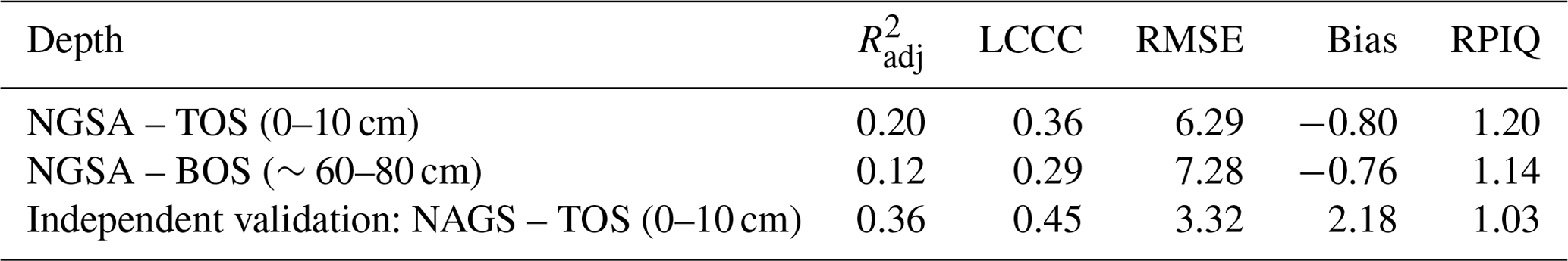
Validation statistics based on internal evaluation using the out-of-bag data for the Li predictions are presented in Table 3. There was a slightly lower accuracy on the prediction for BOS ($R_{\text{adj}}^{\mathrm{2}}=\mathrm{0.12}$; LCCC=0.29; RMSE=7.28 mg kg⁻¹) compared to TOS ($R_{\text{adj}}^{\mathrm{2}}=\mathrm{0.20}$; LCCC=0.36; RMSE=6.29 mg kg⁻¹). This is expected as most of the environmental covariates reflected soil surface conditions. To the best of our knowledge, the machine learning models developed in most mineral exploration studies were assessed based on classification accuracy (i.e. presence or absence of specific minerals in the sample) instead of regression accuracy (Jooshaki et al., 2021). In addition, remote sensing studies on mapping Li minerals are rarely validated (e.g. Cardoso-Fernandes et al., 2019). Hence, no comparison can be made with other studies.

Table 3 Internal model evaluation and validation results for the prediction of Li concentrations using cubist model for both NGSA depths: top outlet sediment (TOS) 0–10 cm and bottom outlet sediment (BOS) ∼60–80 cm. External independent validation is based on comparing predictions to the NAGS dataset Li concentrations.

3.2.2 Independent validation dataset

The predictive model performance was also externally evaluated using an independent dataset (NAGS, TOS only) that was not part of the calibration dataset. To address the analytical variation that could potentially arise from the use of a predictive model from the NGSA dataset for the NAGS dataset, a levelling method was implemented. A subset of the NGSA dataset within the extent of the NAGS dataset was extracted (range = 0.05–28.7 mg kg⁻¹; median = 4.15 mg kg⁻¹) and compared to the NAGS dataset (range = 0.1–19.5 mg kg⁻¹; median = 3 mg kg⁻¹) using a two-sample Kolmogorov–Smirnov test (D=0.24, p<0.01). Because the samples were not deemed to have a similar distribution at a 1 % significance, a correction factor was calculated to level the NAGS dataset to the NGSA dataset using TILL-1 CRM standards. Upon levelling, the two datasets were deemed to have a similar distribution to the two-sample Kolmogorov–Smirnov test (D=0.18, p=0.012).

We reported the performance of model validation the same way the model evaluation was conducted (Table 3 and Fig. 5). The model validation resulted in higher accuracy (R²=0.36; LCCC=0.45). The RMSE was also slightly lower ($\text{RMSE}=\mathrm{3.32}\mathrm{mg}{\mathrm{kg}}^{-\mathrm{1}}$) than that observed in the TOS model evaluation ($\text{RMSE}=\mathrm{6.29}\mathrm{mg}{\mathrm{kg}}^{-\mathrm{1}}$), most likely due to lower observation values within the NAGS validation dataset.

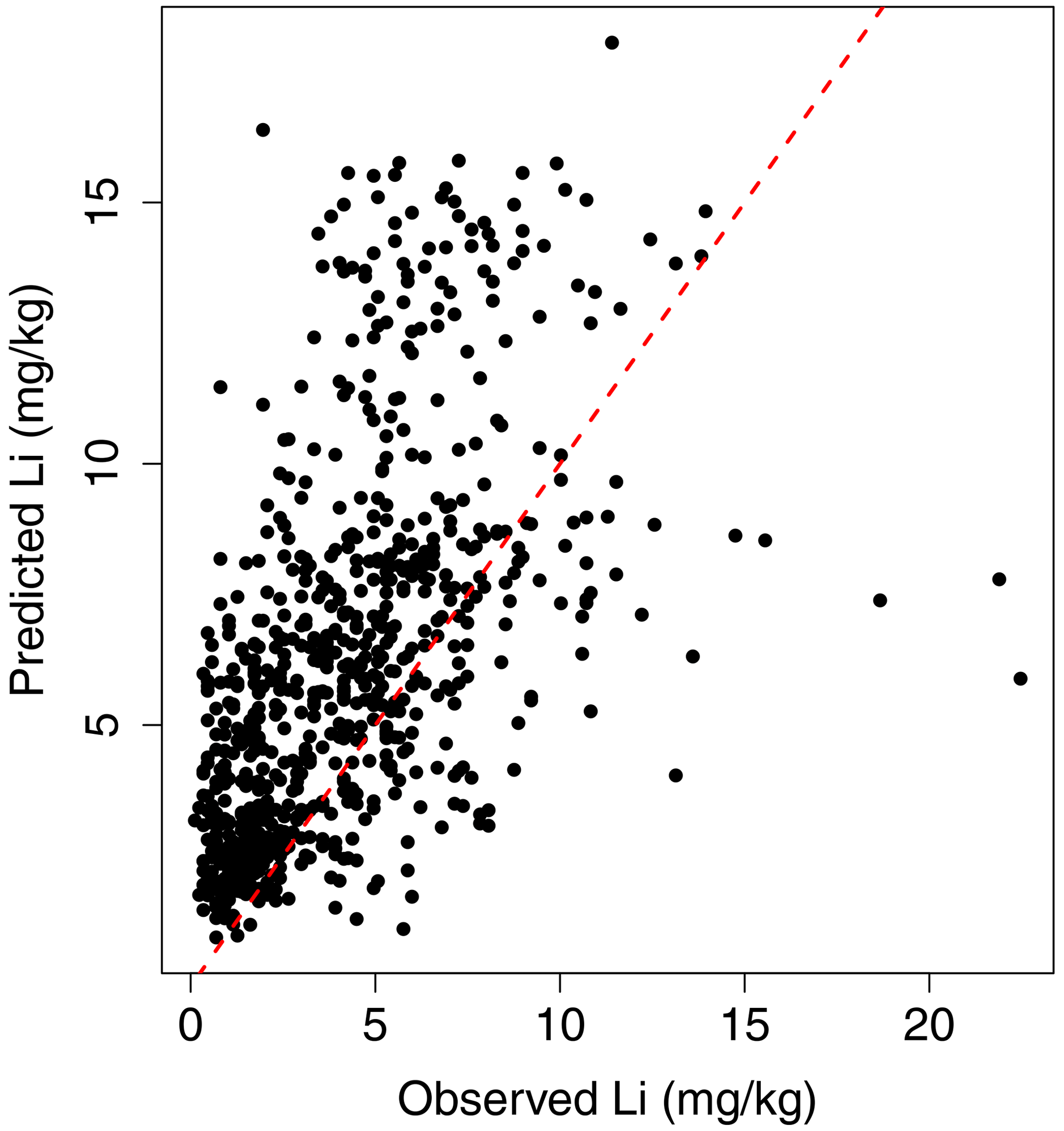
Figure 5 Goodness-of-fit plot showing observed vs. predicted Li concentrations based on the independent validation dataset (NAGS, TOS only). The dashed red line is the 1:1 line.

3.3 Variable importance analysis

From the cubist model, we can infer the relative importance of the covariates by calculating the percentage of times a covariate is being used in the model. The variables used by the cubist model can be further split in terms of “importance as conditions within rule” and “frequency of usage as predictors in models”.

For Li prediction in TOS, the variables clay, PTA, TRA, and EPA are of higher importance in the conditions than other variables (Fig. 6). This implies that the model separates out prediction values based on climate covariates along with clay content. However, within the regression models, the top five variables most frequently used in the regression were the Landsat band 2, band 6, band 1, band 3, and gamma radiometric total dose. The first three Landsat bands (red, green, and blue) and band 6 (SWIR2) have been commonly used to predict soil properties, delineate geological boundaries, and differentiate between vegetation zones (Khorram et al., 2012), while the gamma radiometric dose discriminated the various soil types and their mineral make-up. The next set of covariates were annual precipitation and clay and sand contents, indicating they have lower importance as predictors. As indicated in the correlation analysis, slope was not significant.

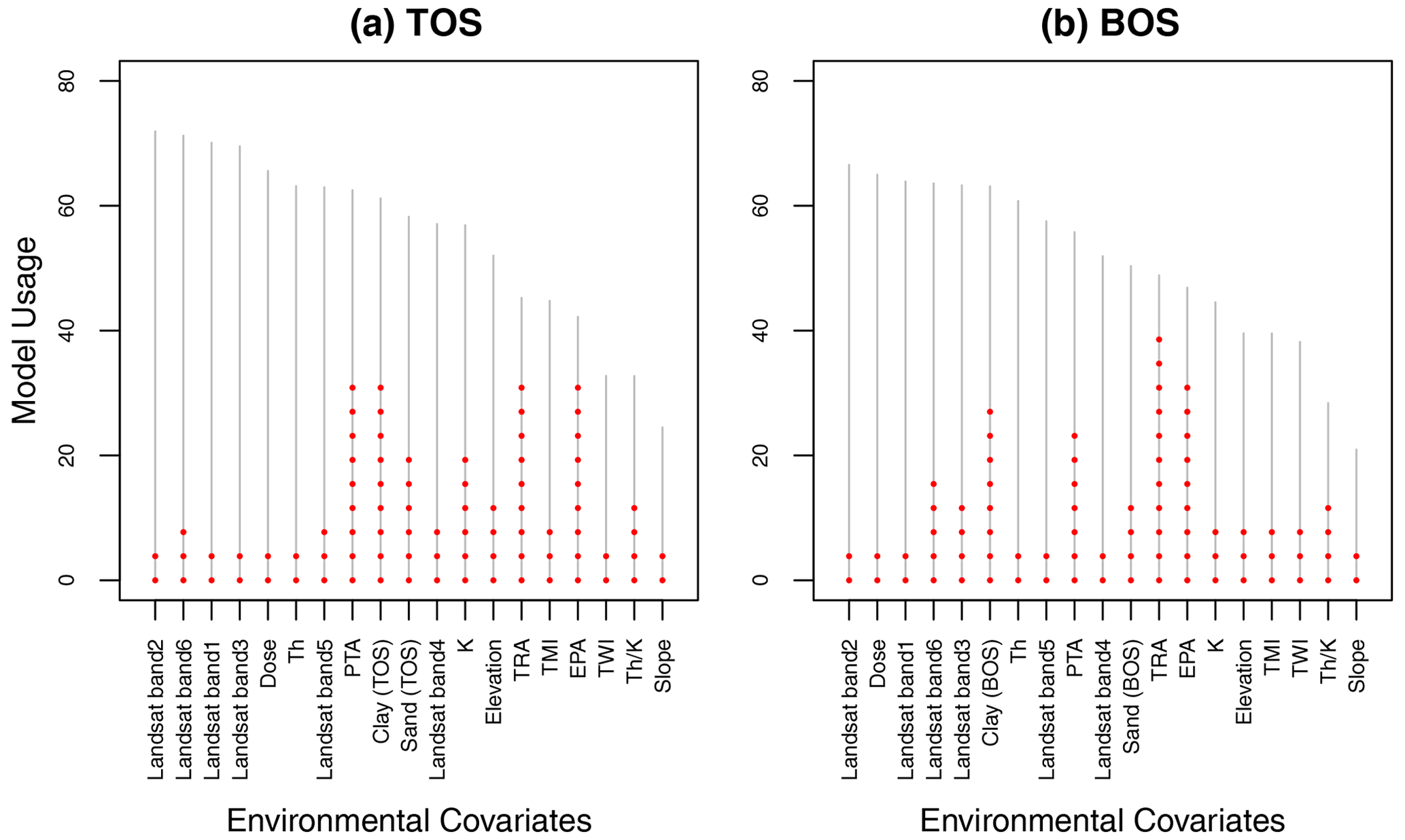
Figure 6 Variable importance of covariates in terms of importance as conditions (dotted red lines) and frequency of usage as predictors (grey lines) by the cubist algorithm for both NGSA depths: top outlet sediment (TOS) 0–10 cm (a) and bottom outlet sediment (BOS) ∼60–80 cm (b). Covariates are sorted in order of decreasing frequency of usage.

For the BOS model, the TRA variable had the highest importance in the conditions of the model (Fig. 6) for Li predictions, separating high and low values. EPA, clay content, and PTA also affect model conditions. Overall, parameters that were more frequently used as predictors in the BOS model were similar to those for TOS, i.e. the top five are gamma radiometric dose and Landsat bands 2, 1, 6, and 3. In the BOS model, however, there was a higher importance of the clay content (sixth most used) compared to the TOS model (ninth). The usage of slope covariate as predictor is similarly low (last) for both TOS and BOS.

3.4 Li prediction maps

The cubist model led to the generation of spatial predictions of aqua-regia-soluble Li concentration in alluvium-derived soils across Australia at two depths (Fig. 7). So far, there are only five known Li mines in Australia (mostly in Western Australia), all of which are located within areas that were predicted to have a higher background concentrations of soil Li, especially for the BOS model ($>\sim \mathrm{8}$ mg kg⁻¹) (Fig. 8).

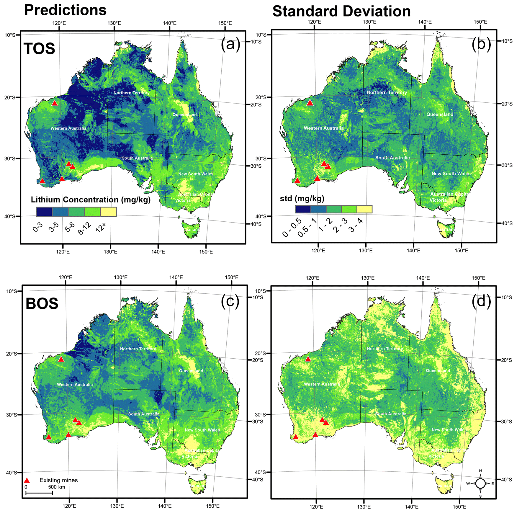
Figure 7 Spatial distributions of predicted aqua-regia-soluble Li concentrations (mg kg⁻¹) in coarse-fraction (<2 mm) alluvial soils across Australia (a, c) and standard deviations (mg kg⁻¹) (b, d) for both National Geochemical Survey of Australia (NGSA) depths: top outlet sediment (TOS) 0–10 cm (a, b) and bottom outlet sediment (BOS) ∼60–80 cm (c, d).

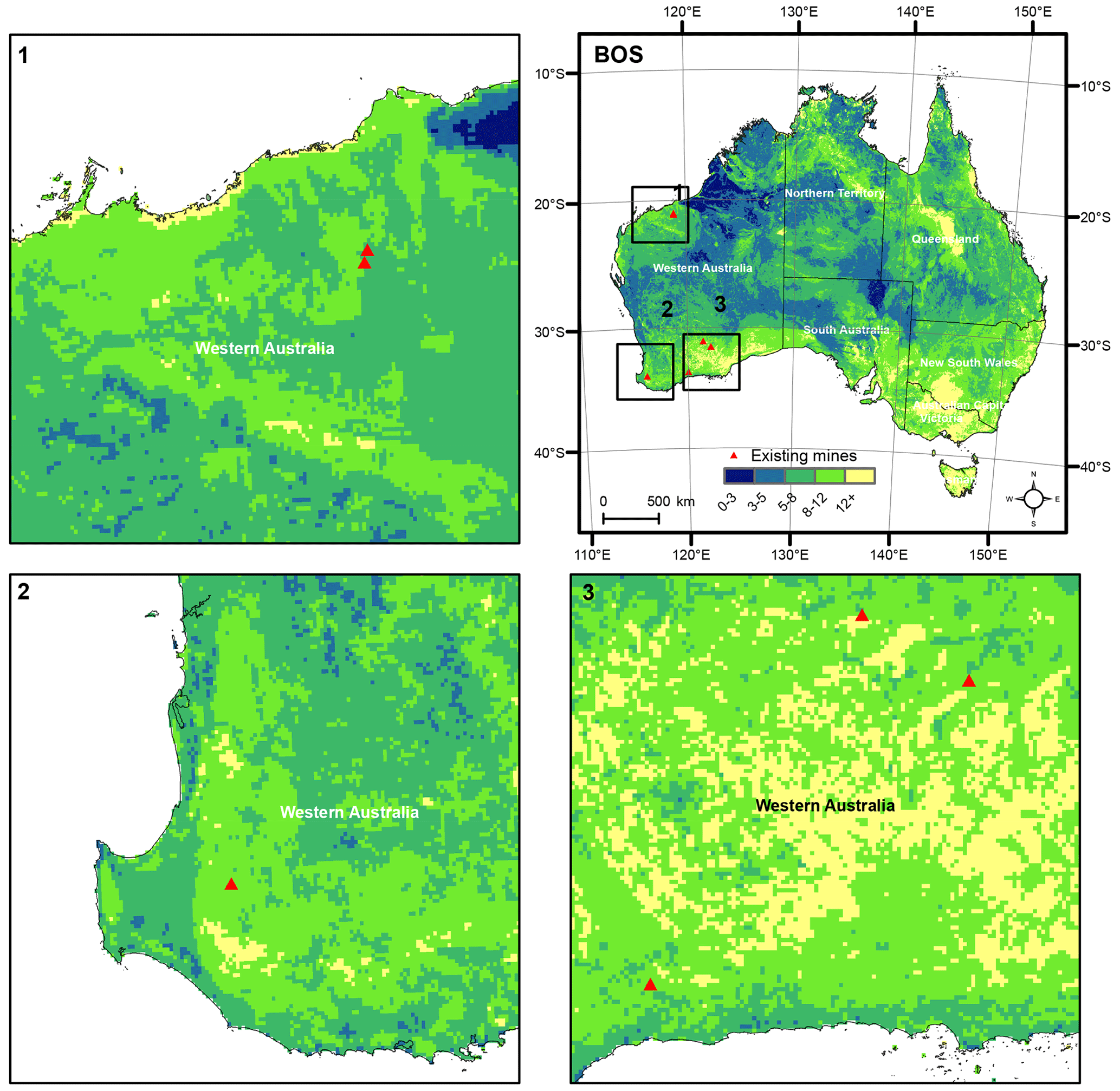
Figure 8 Distribution of Li mines on the digital soil map of Li in Australia for bottom outlet sediment (BOS) ∼60–80 cm depth.

In Australia, the largest producer of spodumene is the Greenbushes Li operation, located approximately 250 km south-southeast of Perth. In the most recent public report, the company reported combined measured and indicated resources of 118.4×10⁶ t (Mt) of ore at 2.4 % Li₂O containing proved and probable reserves of 61.5 Mt at 2.8 % Li₂O (Champion, 2019). Other locations explored for Li include Mount Cattlin and Mount Marion in the Goldfields–Esperance region and Pilgangoora of East Pilbara. In a recent review (Champion, 2019), these projects' reports estimated Li resources ranging from 11.8 to 71.3 Mt at 1.01 % to 1.37 % Li₂O. The predicted soil Li concentrations at the known Li mine sites range from 4.5 to 7.3 mg kg⁻¹ for TOS and from 7.1 to 12.6 mg kg⁻¹ for BOS. The highest TOS and BOS concentrations of Li proximal to a known mine site are for the Mount Marion deposit in Western Australia.

Although most Li exploration to date has been conducted in Western Australia, our map indicates that other regions in Australia are potentially anomalous in Li (Fig. 7). These areas are located for instance within the central western region of Queensland and visually correspond to areas of widespread black cracking (smectite-rich) soils or Vertosols (Isbell, 2021). An elevated concentration of Li was also observed over parts of the Eucla Basin, which has a widespread distribution of Fe-oxide-rich regolith with carbonate accumulations (Johnson, 2015; Wilford et al., 2015). The sources of carbonate include weathered Proterozoic and Palaeozoic carbonate bedrock, vast marine sediments that extend across the low-lying and offshore areas associated with Cenozoic sedimentary basins, and abundant widespread pedogenic carbonates (Johnson, 2015). This is in line with de Vos et al.'s (2006) observations, where higher Li concentrations of up to 56 mg kg⁻¹ were identified in calcareous soil (high carbonate accumulation) in comparison to those of organic soil (1.3 mg kg⁻¹). The Fe in the Fe-oxides and oxyhydroxides that help retain Li may be released from oxidation of primary minerals during weathering (Kabata-Pendias, 2010). The ultimate origin of Li within these clay-, iron-, and carbonate-rich soils remains to be established in the case of Australia. Other regions of potential interest occurring in different soil types are located in southern New South Wales and parts of Victoria.

We further explored the correlation of Li concentration against soil orders (Searle, 2021). Figure 9 shows the range of Li concentrations across various soil types identified at the sampling locations. The Li concentration tended to be slightly higher in Vertosols, Calcarosols, and Dermosols. These observations indicate Li accumulated in a more uniform soil profile with less differentiation between top and subsoils. In addition, clay soils (Vertosols) and soils with high CaCO₃ (Calcarosols) appeared to have larger Li concentrations. These observations supported the anomalous Li predictions in various parts of Australia mentioned earlier.

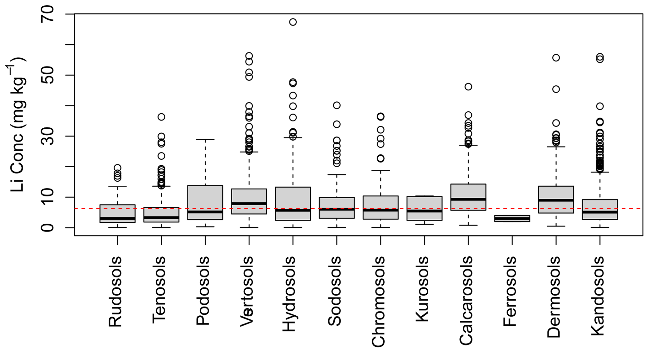
Figure 9 Boxplots of Li concentration in both TOS and BOS across various soil orders based on the Australian Soil Classification (ASC) system. The boxes indicate the interquartile interval, the bold black lines in the middle of the boxes represent the median, and the values outside 1.5 times the interquartile interval are indicated by circles. The dashed red line represents the median values of Li across both TOS and BOS depths.

The highest predicted values on the Li digital soil maps are 28 and 22 mg kg⁻¹ in TOS and BOS, respectively. Although a higher Li concentration was expected to be observed in the deeper layer, the model used in this study was not able to support such predictions yet. This is most likely because the covariates used within the model represent observations from TOS instead of BOS. The variance of covariates within BOS was not obtained, hence yielding lower-accuracy predictions.

3.5 Study limitations

While we have successfully modelled soil Li distribution in Australia and validated it using an independent sample dataset, we recognise that there are limitations to this study's approach. (1) The NGSA data used apply to catchment outlet sediment representing the local accumulation of mainly detrital minerals. Therefore, strictly speaking, the predictions developed herein apply only to similar alluvial soils. (2) The NGSA data were measured using an aqua regia digestion that only extracts a portion of the total Li found in soil. The results could potentially be improved if total Li was measured. Most of the observations collected had a relatively low concentration; having more representative samples at higher concentrations might improve the prediction accuracy. (3) Despite the large amount and spread of data, the NGSA does not cover the whole of Australia. Notably, there is a data gap in parts of Western Australia and South Australia. However, no more extensive geochemical dataset than the NGSA exists in Australia. (4) The environmental covariates used in the study were selected based on our understanding of relevant soil-forming processes. (5) There is also limited information on how the covariates vary with depth except for the soil texture (sand and clay content) data. The inclusion of more environmental covariates related to depth and soil mineralogical information may improve the predictive capability of these machine learning models. Note that quantitative mineralogical data are currently being acquired on the NGSA samples, both as X-ray diffraction data on whole sediment samples and clay fractions (de Caritat and Troitzsch, 2021) and as automated mineralogy using energy dispersive spectrometry on heavy mineral fractions (de Caritat et al., 2022a, b, c).

The final product was only validated in one area within Australia (Tennant Creek–Mount Isa region in the Northern Territory and Queensland). Despite our predictions of elevated soil Li in parts of Queensland, New South Wales, and Victoria, ground-truthing is required to confirm them, and further work is necessary to determine the origin of the contained Li.

4 Data availability

The Li geochemical data for calibration and validation are available at https://doi.org/10.11636/Record.2011.020 (de Caritat and Cooper, 2011b) and https://doi.org/10.11636/Record.2019.002 (Main et al., 2019), respectively. The covariate data used for this study were sourced from the Terrestrial Ecosystem Research Network (TERN) infrastructure, which is enabled by the Australian Government's National Collaborative Research Infrastructure Strategy (NCRIS; https://esoil.io/TERNLandscapes/Public/Products/TERN/Covariates/Mosaics/90m/, last access: 6 December 2022; TERN, 2019). The final predictive map is available at https://doi.org/10.5281/zenodo.7895482 (Ng et al., 2023).

5 Conclusions

Spatial prediction models have been increasingly utilised to help minimise risk and thus cost of mineral exploration. In this study, digital soil mapping of Li concentrations at two different depths (TOS: 0–10 cm; BOS: ∼60–80 cm) based on the cubist model was carried out across Australia using the National Geochemical Survey of Australia dataset and publicly available environmental covariates. Geology and mineralogy are of high importance in predicting soil Li anomalies, as demonstrated by the reliance of the model on the Landsat and gamma-ray radiometric covariates. Despite most mineral exploration for Li being conducted in Western Australia, other regions (such as Queensland, New South Wales, and Victoria) have elevated predicted Li concentrations and could become potential areas of interest. The model accuracy tested on the independent Northern Australia Geochemical Survey (TOS only) was reasonable compared to the calibration model performance. Overall, the model performance was on the low side, and the inclusion of the results into a prospectivity framework needs to consider the model uncertainties. This approach provides an estimate of the environmental background concentration of Li, which is reflecting a range of processes including source rock geochemistry from which the sediments were derived, weathering (including pedogenesis), and geomorphic processes. The work provides a framework to better understand the processes controlling the Li concentration at the surface (as revealed through the covariate relationships), and the modelling effectively delineates regions with locally higher Li background. Despite the low prediction accuracy, this paper demonstrates a step forward in the development of machine learning in generating predictive geochemical maps. It also highlights the importance of the establishment of national geochemical survey databases enabling the exploration of various elements and minerals nationally and globally, as well as not being limited to Li. Future work should include obtaining other relevant environmental covariates and new mineralogy data, which could further improve model performance; ground-truthing anomalous regions; and investigating ultimate Li sources. As more survey data are collected, the use of more complex models can also be explored, including the use of Li concentrations in bedrock materials.