An improved global land cover mapping in 2015 with 30 m resolution (GLC-2015) based on a multisource product-fusion approach

Global land cover (GLC) information with fine spatial resolution is a fundamental data input for studies on biogeochemical cycles of the Earth system and global climate change. Although there are several public GLC products with 30 m resolution, considerable inconsistencies were found among them, especially in fragmented regions and transition zones, which brings great uncertainties to various application tasks. In this paper, we developed an improved global land cover map in 2015 with 30 m resolution (GLC-2015) by fusing multiple existing land cover (LC) products based on the Dempster–Shafer theory of evidence (DSET). Firstly, we used more than 160 000 global point-based samples to locally evaluate the reliability of the input products for each land cover class within each 4^∘ × 4^∘ geographical grid for the establishment of the basic probability assignment (BPA) function. Then, Dempster's rule of combination was used for each 30 m pixel to derive the combined probability mass of each possible land cover class from all the candidate maps. Finally, each pixel was determined with a land cover class based on a decision rule. Through this fusing process, each pixel is expected to be assigned the land cover class that contributes to achieving a higher accuracy. We assessed our product separately with 34 711 global point-based samples and 201 global patch-based samples. Results show that the GLC-2015 map achieved the highest mapping performance globally, continentally, and ecoregionally compared with the existing 30 m GLC maps, with an overall accuracy of 79.5 % (83.6 %) and a kappa coefficient of 0.757 (0.566) against the point-based (patch-based) validation samples. Additionally, we found that the GLC-2015 map showed substantial outperformance in the areas of inconsistency, with an accuracy improvement of 19.3 %–28.0 % in areas of moderate inconsistency and 27.5 %–29.7 % in areas of high inconsistency. Hopefully, this improved GLC-2015 product can be applied to reduce uncertainties in the research on global environmental changes, ecosystem service assessments, and hazard damage evaluations. The GLC-2015 map developed in this study is available at https://doi.org/10.6084/m9.figshare.22358143.v2 (Li et al., 2023).

1 Introduction

Land cover (LC), influenced by both nature and human activities (Running, 2008; Gong et al., 2013; Song et al., 2018; H. Liu et al., 2021), is a significant component of the Earth system (Yang and Huang, 2021). Global land cover (GLC) products can serve as fundamental data for various studies, such as climate and environmental changes (Bounoua et al., 2002; Foley et al., 2005; Grimm et al., 2008; Yang et al., 2013; Schewe et al., 2019), food security (Verburg et al., 2013; Ban et al., 2015), carbon cycling (Moody and Woodcock, 1994; Defries et al., 2002; Gómez et al., 2016), biodiversity conservation (Chapin et al., 2000; Giri et al., 2005), and land management (Mayaux et al., 2004; Verburg et al., 2011). Therefore, there is a pressing need for a detailed, accurate, and high-quality GLC product to support global change research and sustainable development.

In the preliminary stage, LC mapping mainly relied on visual interpretation, which is time-consuming, labor-intensive, and difficult to apply at the global scale (Gong, 2012). In recent decades, satellite remote-sensing data, which can provide information on large-area coverage and long-term monitoring, have been adopted to generate GLC products. With coarse-resolution satellite data such as the Advanced Very High Resolution Radiometer (AVHRR), Moderate Resolution Imaging Spectroradiometer (MODIS), Medium Resolution Imaging Spectrometer (MERIS), and Global Land Surface Satellite (GLASS), a variety of GLC products have been developed at 5 km to 300 m resolution (Loveland et al., 2000; Hansen et al., 2000; Bartholomé and Belward, 2005; Friedl et al., 2010; Defourny et al., 2018; H. Liu et al., 2020). Although these GLC products have been widely applied to many applications, it has been proven that the differences between sensors, classification systems, and considerably low accuracies in areas prevent harmonization of these products (Herold et al., 2008; Verburg et al., 2011; Grekousis et al., 2015). Also, these products are far from providing enough fine spatial details of LC due to their relatively coarse spatial resolution, which does not meet the demands of many studies (Giri et al., 2013; Yang et al., 2017). To allow research which can capture most human activity, finer-resolution (e.g., 30 m) GLC products are required (Giri et al., 2013).

With the free accessibility of high-resolution satellite remote-sensing data, GLC mapping at fine resolution has been successfully conducted. Using Landsat imagery, there has been a milestone achievement in that the two GLC products are generated with a fine resolution of 30 m, namely, the Finer Resolution Observation and Monitoring of Global Land Cover product (FROM_GLC) (Gong et al., 2013) and Globeland30 (Chen et al., 2015). After that, a 30 m resolution GLC mapping in 2017 was achieved using the first all-season sample set (Li et al., 2017). More recently, Zhang et al. (2021) used both Landsat time series imagery and high-quality training data from the Global Spatial Temporal Spectra Library (GSPECLib) to produce a 30 m GLC map in 2015 (GLC_FCS30) with a two-level classification scheme. Several attempts have been made to improve the accuracy of 30 m GLC products which are prevalent in the generation of the GLC mapping task over the last few years. FROM_GLC was created by employing four classification algorithms to classify the Landsat images and choosing time series of MODIS EVI data for training and testing. Globeland30 was created by proposing a pixel-object-knowledge-based (POK) method to ensure consistency and accuracy. GLC_FCS30 was generated by adopting local adaptive random forest models with high-quality training samples derived from the GSPECLib. Globeland30, FROM_GLC, and GLC_FCS30 are excellent and indispensable GLC products which have contributed much to various research, such as biodiversity conservation (Wu et al., 2020; Meng et al., 2023), climate change (Kim et al., 2016; Xue et al., 2021; Zheng et al., 2022), and land management (Shafizadeh-Moghadam et al., 2019). In addition to these multiple-class GLC products, GLC products for individual LC classes, such as cropland (Yu et al., 2013; Lu et al., 2020), forest (Hansen et al., 2013; Shimada et al., 2014; Zhang et al., 2020), wetland (Hu et al., 2017; Zhang et al., 2023), water (Liao et al., 2014; Pekel et al., 2016; Pickens et al., 2020), and impervious surfaces (Gong et al., 2020; Huang et al., 2021, 2022; X. Liu et al., 2020), have been successfully generated.

Despite the great efforts in producing more accurate products, the existing 30 m GLC products still show unstable performance in certain LC classes and some specific areas (Sun et al., 2016; Kang et al., 2020). Furthermore, the existing 30 m products showed great agreement in overall spatial distribution patterns but significant spatial inconsistency in some specific areas (heterogeneous areas and transition zones) and spectrally similar classes (forest and shrubland, cropland and grassland) (Gao et al., 2020; L. Liu et al., 2021). The spatial inconsistency between the existing 30 m GLC products resulted from differences in their classification systems, classification techniques employed, source data, and spatial distributions and sizes of training samples (Yang et al., 2017; Gao et al., 2020). Due to the aforesaid limitations, users of GLC products still have difficulties in an appropriate selection of data for their specific application. Ultimately, this situation leads to uncertainties in outcomes of related studies when different 30 m GLC products are used. For GLC mapping with fine spatial resolution, more efforts should be focused on improving the mapping in heterogenous and fragmented landscapes (Herold et al., 2008; L. Liu et al., 2021). Therefore, it is pressing to generate a more accurate and reliable GLC product with high classification accuracy, especially for spatially inconsistent regions and low-accuracy LC classes.

According to Gong et al. (2016), inconsistencies between LC products indicate available complementary information, and more robust and reliable data can be generated by integrating the input maps with the data-fusion method. Given that different maps have disagreement and provide accurate information in different locations, we can make a best choice for the class label assigned to each pixel by weighting the credibility of all the available information and combining them through a decision rule (Clinton et al., 2015). In this way, the output map of integration on input maps can reduce the overall risk of assigning a wrong class label to a pixel and at least achieve the average performance of input maps. Several attempts have been made to produce an accurate and consistent LC map using various methods, such as majority voting (MV), fuzzy agreement, and Bayesian theory. Iwao et al. (2011) created a GLC map based on a simple majority voting method. Jung et al. (2006) generated a 1 km GLC map by combination of MODIS, GLC2000, and GLCC data based on fuzzy agreement scoring. Subsequently, Fritz et al. (2011) extended the synergy method of Jung et al. (2006) by ranking LC maps and mapped the cropland extent in sub-Saharan Africa. See et al. (2015) generated two GLC products by integrating medium-resolution LC products with geographically weighted regression (GWR). Gengler and Bogaert (2018) proposed a Bayesian data-fusion method and applied it to the LC mapping for a specific region in Belgium. All these studies have demonstrated that the fusion method can create an integrated LC product where the mapping accuracy is greatly improved by combining the best of the candidate maps. However, the MV method is sensitive to the quality of the candidate maps and has significant uncertainties when the input products exhibit great disagreement (Chen and Venkataramanan, 2005). The fuzzy agreement is highly subjective since it depends on expert assessment, while the Bayesian theory requires prior knowledge or conditional probabilities and fails to handle the states of ignorance (Liu and Xu, 2021).

The Dempster–Shafer theory of evidence (DSET) is an evidence-based approach to reason with uncertainties. Unlike the majority voting, the DSET method can discount evidence from inaccurate information with a probability mass that reflects the degree of belief rather than a binary decision (Razi et al., 2019). In contrast to the Bayesian theory, the DSET can integrate evidence from a variety of sources without the requirement of prior knowledge (Chen and Venkataramanan, 2005). Moreover, the reliability of the final fused results based on the DSET method is measured with a total degree of belief. Although previous literature focused on the application of the DSET method in multisource data aggregation, very little research has been conducted globally due to the lack of accurate and sufficient samples and the demand for adequate computing resources.

In this research, we propose a multisource product-fusion approach on the Google Earth Engine (GEE) platform to produce an improved GLC product in 2015 (GLC-2015) with 30 m resolution. The fusion approach we proposed aims to deal with the inconsistency between previous 30 m GLC products and generate a map which has better mapping performance than any of the candidate maps by evaluating the mapping accuracy of these existing products at the local scale and choosing the most credible LC class. To fulfill the purpose, we first performed reliability evaluation, where the accuracy of each product for each LC class in each 4^∘ × 4^∘ geographical grid is regarded as the evidential probability of creating the basic probability assignment (BPA) function. Then, the BPA values of all the LC classes from different products were fused according to Dempster's rule of combination. Finally, the GLC-2015 map was integrated after a final accepted LC class with the maximum combined probability mass was assigned to each 30 m pixel. The GLC-2015 map was separately validated with two different validation sets, namely, global point-based samples and global patch-based samples, and compared with the existing products. Moreover, we provided an analysis for the mapping improvement of GLC-2015 compared to other GLC products in areas of high mapping inconsistency. The GLC-2015 map is proven to be accurate and credible and can significantly improve the mapping accuracy in areas of high inconsistency.

2 Datasets

2.1 Multiple-class GLC products

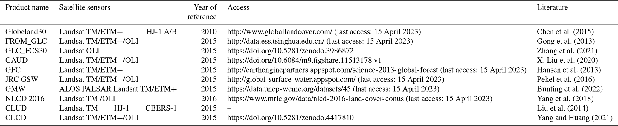
Three existing 30 m GLC products with multiple classes, including GlobeLand30, FROM_GLC, and GLC_FCS30, were employed as input maps in the fusion based on the DSET. A summary of their detailed information is shown in Table 1.

GlobeLand30, a widely used global geoinformation product, was produced by the POK-based method using Landsat and HJ-1 satellite images. Globeland30 products are freely accessible online at the website (http://www.globalland30.org, last access: 15 April 2023) for 2000 and 2010. From the accuracy assessment, Globeland30 for the year 2010 had an overall accuracy exceeding 80.0 % using large samples (Chen et al., 2015). Although the data time of GlobeLand30 is 2010, which has a 5-year gap with other products, it was used because the changed areas of LC caused by the time interval are tiny compared to the global land area. In addition, there is relatively less uncertainty due to LC changes than due to inaccurate classification (Xu et al., 2014). Most spatial disagreements between the existing maps are about classification errors rather than LC changes over the time interval (McCallum et al., 2006; See et al., 2015).

FROM_GLC, the first 30 m GLC product generated using numerous Landsat images, has a fine classification system with a two-level structure. It achieved an overall accuracy (OA) of 64.5 % through validation with the complete test samples and 71.5 % with a subset of test samples in homogeneous areas (Gong et al., 2013).

GLC_FCS30 was developed using Landsat time series data and large training samples from the GSPECLib. It has a two-level classification scheme that contains 16 global LCCS LC classes and 14 detailed regional LC classes. The overall accuracy of GLC_FCS30 according to the LCCS level-1 validation scheme reached 71.4 % (Zhang et al., 2021).

Table 1 Detailed information on GLC products and national-scale LC products used in this paper.

2.2 Single-class GLC products

To improve the quality of the fusing result, a set of highly qualified GLC products with a single class at 30 m fine resolution were also used. Compared to the multiple-class GLC products, these single-class GLC products are more likely to provide accurate information since they usually focus on promoting the mapping performance of a specific LC class. These products include Global Forest Change (GFC) (Hansen et al., 2013), Global Annual Urban Dynamics (GAUD) (X. Liu et al., 2020), the Joint Research Centre's Global Surface Water (JRC GSW) (Pekel et al., 2016), and the Global Mangrove Watch (GMW) (Bunting et al., 2022). While these single-class products are either annual or multi-epoch, we only selected these products in the target year of 2015. The background information of these single-class products was considered another land cover class (e.g., non-water) participating in the fusion. The accuracy of the background information was defaulted to 0 since it did not provide information about any of the other nine categories in our classification system. Table 1 also describes the information of these selected single-class GLC products.

GFC resulted from a time series analysis of growing season Landsat scenes, aiming to provide information about global tree cover extent, gain, and loss at a 30 m spatial resolution. The accuracy assessment was performed at global and climate domain scales, the forest gain reached an overall accuracy of 99.6 %, and the forest loss reached 99.7 % across the globe (Hansen et al., 2013). Up to now, it had a temporary coverage from 2000 to 2020.

GAUD, which provides 30 m annual urban extent for the time period of 1985 to 2015, was generated using numerous Landsat images with both a data-fusion approach and a temporal segmentation approach on the GEE platform. Validation was conducted across different urban ecoregions and the globe by the product developer. The accuracy of mapping an urbanized year was 76.0 % for the period of 1985 to 2000 and 82.0 % for the period of 2000 to 2015 in humid regions worldwide (X. Liu et al., 2020).

The JRC GSW dataset provides a monthly presentation of global surface water changes from 1984 to 2015 at a fine 30 m resolution. Expert systems, visual analytics, and evidential reasoning were exploited to detect water extent and changes. Based on 40 124 validation points over the globe and across the 32 years, commission accuracies were determined with overall accuracies of 99.45 % (Thematic Mapper – TM), 99.35 % (Enhanced Thematic Mapper Plus – ETM+), and 99.54 % (OLI – Operational Land Imager), and omission accuracies were reflected in overall accuracies of 97.01 % (TM), 95.79 % (ETM+), and 96.25 % (OLI) (Pekel et al., 2016). We used the GSW Yearly Water Classification History v1.1 in the GEE catalog. A single “waterClass” band is present in each image that provides the water's seasonality throughout the year with four types: no data, no water, seasonal water, and permanent water. Since the seasonal water in GSW data is not as reliable as the permanent water (Meyer et al., 2020), we selected permanent water bodies and excluded seasonal water bodies.

The GMW dataset was produced as a result of the GMW initiative, which aims to provide consistent information on mangrove extent. The global mangrove map in 2010 was generated as a baseline map employing the Extremely Randomized Trees classifier to classify the Advanced Land Observing Satellite (ALOS) Phased-Array L-band Synthetic Aperture Radar (PALSAR) and Landsat imagery. Assessed by a total of 53 878 sample points globally, the overall accuracy of the baseline map reached 95.3 %, and the producer's accuracy achieved 94.0 % (Bunting et al., 2018). Based on the baseline in 2010, mangrove extent maps for six epochs between 1996 and 2016 have been established, and annual change monitoring from 2018 and onwards is undertaken.

2.3 National-scale LC products

Land cover products which focus on a national scale are more likely to possess higher accuracy because they were produced by experts who have good knowledge of land cover classes nationally. Thus, the National Land Cover Database 2016 (NLCD 2016) for the year 2016 over the conterminous United States (CONUS) (Yang et al., 2018), China's land-use/cover dataset (CLUD) (Liu et al., 2014) for 2015, and the annual China land cover dataset (CLCD) (Yang and Huang, 2021) for 2015 were also included in the fusion. The detailed information on these national-scale products is listed in Table 1.

The NLCD 2016 database, which provides continuous and accurate information on land cover and change from 2001 to 2016 at an interval of 2 or 3 years, was produced based on a pixel- and object-based approach and an effective post-classification process (Yang et al., 2018). The level-1 and level-2 overall accuracy of the NLCD 2016 database for 2016 was 90.6 % and 86.4 % for the CONUS, respectively (Wickham et al., 2021). CLUD, developed by the digital interpretation method using Landsat images, provides land cover information over China from 1980s to 2015. The overall accuracy of CLUD reached 94.3 % and 91.2 % for level-1 and level-2 land cover classes, respectively (Liu et al., 2014). CLCD was generated with stable training samples derived from CLUD and Landsat time series. Assessed with 5463 validation samples, CLCD obtained an overall accuracy of 79.31 % (Yang and Huang, 2021).

2.4 Global point-based and patch-based samples

In this study, we collected two sets of global samples, namely, the global point-based samples and the global patch-based samples. To collect representative and sufficient samples efficiently, we divided the world's terrestrial area into 4^∘ × 4^∘ geographical grids. A total of 1507 grids are distributed evenly across the globe, shown as Fig. 1.

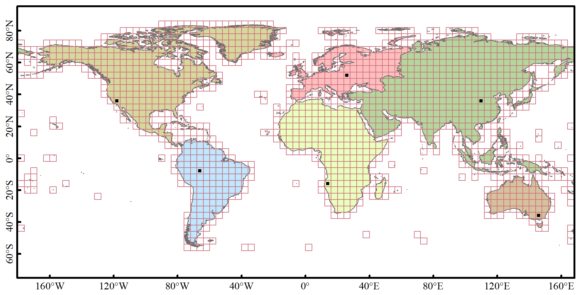
Figure 1 Spatial distribution of the 4^∘ × 4^∘ geographical grids over the world. Six black rectangle tiles with a size of 0.25^∘ were used for visual comparison between our product and the other three products.

To derive the global point-based samples, we adopted stratified random sampling in each grid. The stratified random sampling depends on the area ratio of classes from a land cover product. We used FROM_GLC as prior knowledge rather than Globeland30 and GLC_FCS30 with two considerations. (1) FROM_GLC has the same data time as our target map (GLC-2015), while Globeland30 has a 5-year interval from our samples, which affects the sizes of samples for each LC class. (2) The 10 level-1 land cover classes of FROM_GLC are similar to that in the classification system of GLC-2015, while GLC_FCS30 has differences from GLC-2015 in the classification scheme and definition of land cover classes. First, the FROM_GLC product was used to calculate the area ratio of each LC class. Then, points were randomly extracted from FROM_GLC according to the area ratio and spatial location of each class. Finally, more than 200 000 global samples were collected. Through the sampling method mentioned above, the global point-based samples were even across the globe and sufficient for each class in each grid. Therefore, more than 50 points could be easily derived for classes with a small area ratio in the 4^∘ × 4^∘ grid. FROM_GLC shows low accuracy for some LC classes, especially for cropland and forest (Gao et al., 2020; L. Liu et al., 2021; Zhang et al., 2021, 2022). If the global samples were extracted with the LC class label from FROM_GLC, there would be inevitable errors. Therefore, FROM_GLC was only used to determine the sizes and locations of samples for each class. Instead, all the points were manually labeled according to Google Earth high-resolution images. The whole sample set was randomly split into two subsets: 80 % of the global samples were used to assess the accuracy of each GLC product for various LC classes at the global scale and in each grid. The remaining 20 % were used for the validation of the GLC-2015 map and data intercomparison between different products. Figure 2 presents the distribution of the whole global point-based samples and the subset for accuracy assessment and data intercomparison.

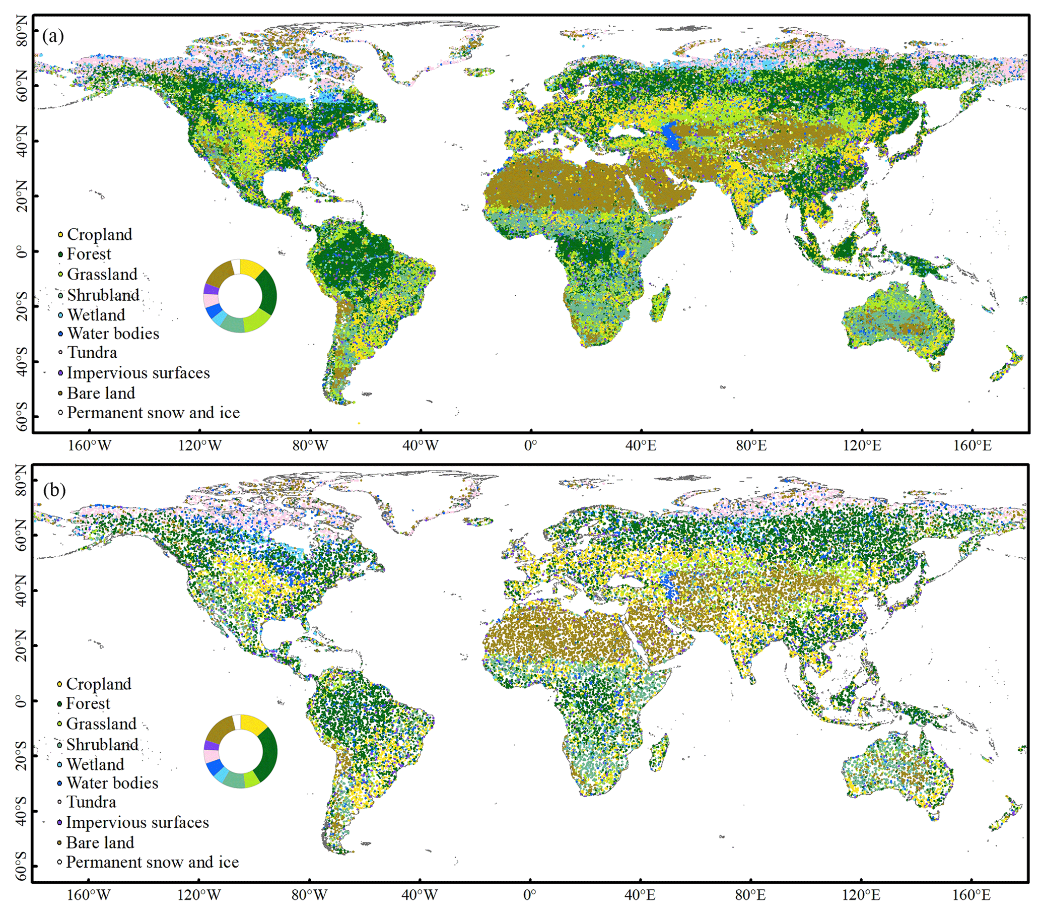
Figure 2 Spatial distribution of (a) the global point-based samples and (b) the subset of the global point-based samples for accuracy assessment and data intercomparison; the proportions of each LC class are shown in the pie chart.

To verify the consistency between GLC-2015 and the actual pattern of the landscape at the local scale, we also established the global patch-based samples. Simple random sampling was used to derive 5 km × 5 km blocks over the world's terrestrial area and across different ecoregions because it is easy to perform and capable of augmenting the sample size from target areas (Pengra et al., 2020). Since inconsistency between current GLC maps tends to appear in the heterogeneous areas, such as fragmented regions and transition zones, we slightly increased the sample size for areas with the heterogeneous landscape to better evaluate our mapping results. In total, there were 201 blocks selected as the global patch-based samples, as displayed in Fig. 3a. Then, for each block in the patch-based samples, we used ArcGIS 10.5 software to derive polygons (patches) of various sizes which captured the real landscape on the high-resolution images. Meanwhile, each polygon was manually labeled with a LC class. Four examples of producing patch-based samples are shown in Fig. 3b and c.

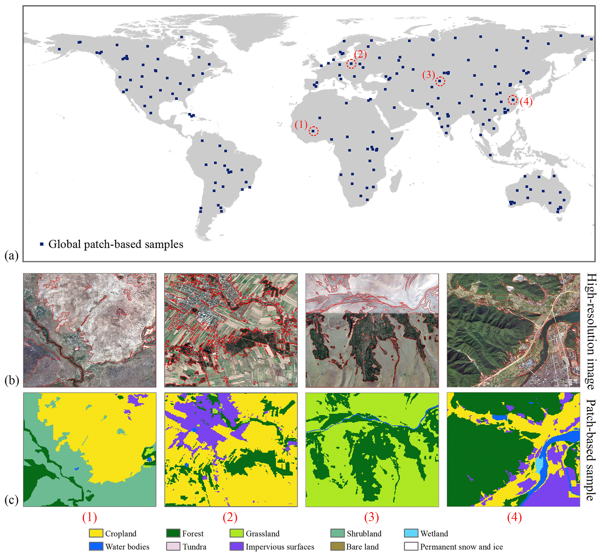
Figure 3 Spatial distribution and selected examples of the global patch-based samples. The locations of 5 km × 5 km patch-based samples are shown as panel (a), and the locations of the four selected samples are shown by red dash circles. Panels (b) and (c) illustrate the production of global patch-based samples on manual interpretation. The red lines in high-resolution images circa 2015 result from vectorization using ArcGIS 10.5 software. Four corresponding patch-based samples are shown as panel (c).

3 Methods

In this study, we proposed a multisource product-fusion method to produce the GLC-2015 map. The procedure mainly comprised the fusion based on the Dempster–Shafer theory of evidence (DSET), accuracy assessment, and data intercomparison as shown in Fig. 4. The basis of this study is the fusion of multisource products based on the DSET. The fusion method was performed at the pixel level, and it involves the following three main steps. (1) Construct the BPA function of each pixel that belongs to each LC class considering the accuracy assessment of various products. (2) Calculate the combined probability mass for each class per pixel using Dempster's rule of combination. (3) Determine the finally accepted LC class per pixel by a decision rule. Afterwards, pixels with a determined LC class were integrated to generate a new map. For large-scale or global land cover mapping, previous researchers divided the study area into a lot of subregions and conducted classification in each subregion on GEE (Gong et al., 2020; X. Liu et al., 2020; Huang et al., 2021; Jin et al., 2022; Zhang et al., 2021; Zhao et al., 2021). The shape and size of the subregion vary in previous work, such as hexagons with a side length of 2^∘ and geographical grids with sizes of 1^∘ × 1^∘, 3.5^∘ × 3.5^∘, 5^∘ × 5^∘, or 10^∘ × 10^∘. When deciding on the sizes of subregions, two important factors should be considered. The sizes of samples in each subregion should be sufficient so that the rare land cover classes will not be missed. On the other hand, it is impossible to implement mapping work in a subregion as large as we want due to memory constraints. To determine the appropriate size, we tested different sizes of the subregion (see Table S1 in the Supplement). The result shows that dividing the study area into 4^∘ × 4^∘ grids performed best. Therefore, we split the world's terrestrial area into 1507 4^∘ × 4^∘ geographical grids. The entire framework was implemented in all 4^∘ × 4^∘ geographical grids on the GEE platform.

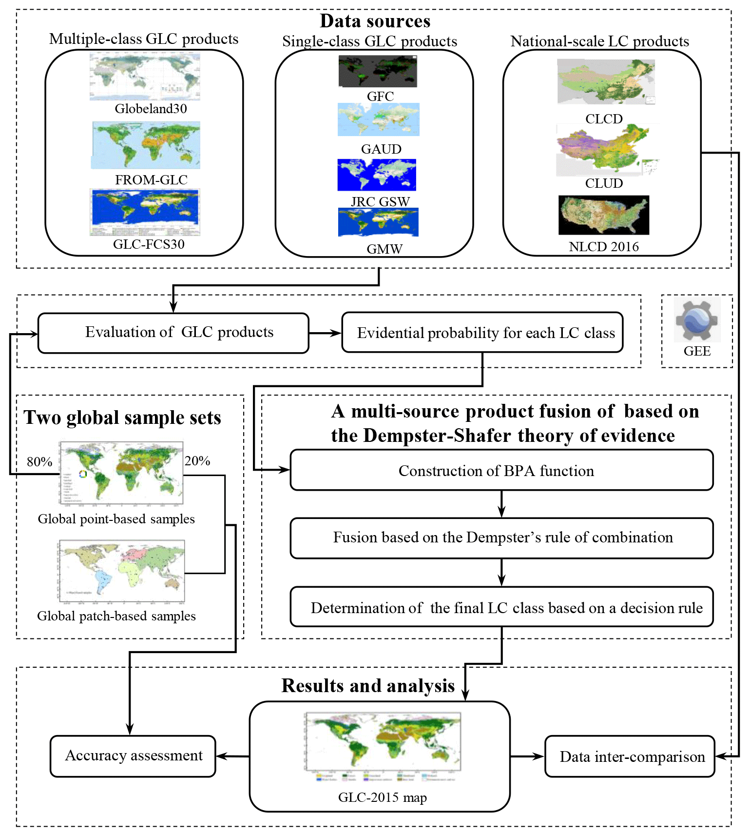
Figure 4 The framework for generating the GLC-2015 map using a multisource product-fusion approach based on the DEST.

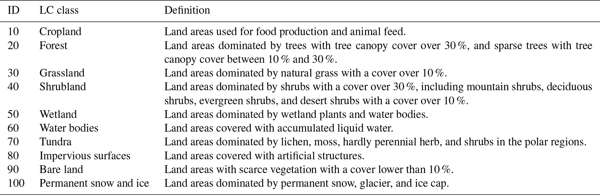
3.1 Definition of the classification system

In this study, we adopted the classification system with 10 LC classes, including cropland, forest, grassland, shrubland, wetland, water bodies, tundra, impervious surfaces, bare land, and permanent snow and ice (Chen et al., 2015), as listed in Table 2. Due to the applications for different social needs, the existing GLC products and national-scale LC products were produced with different classification systems (Tables S2–S3). GlobeLand30 used a simple classification system that only contained 10 first-level classes. Unlike GlobeLand30, FROM_GLC and GLC_FCS30 were classified with a two-level classification scheme. Through analysis of these systems, we found that the classification systems are not the same, but they have some agreements. There are both 10 major classes in GlobeLand30 and FROM_GLC despite the fact that the definitions of some classes differ. Additionally, in contrast to GlobeLand30 and FROM_GLC, the level-0 classification system of GLC_FCS30 lacks tundra. However, in the level-2 detailed LC classes of GLC_FCS30, lichens and mosses have little distinction from tundra.

According to the LC translation tables (Tables S2–S3), the original LC classes of FROM_GLC and GLC_FCS30, CLUD for 2015, and NLCD 2016 for 2016 were converted into the 10 target land cover classes based on the similarity of LC definition. Note that cropland in our classification system was defined as land areas for food production and animal feed. Therefore, pasture in level-2 classes of FROM_GLC was converted into cropland rather than grassland. In addition, lichens/mosses in the level-2 detailed classification system of GLC_FCS30 were converted into tundra.

Table 2 Classification system adopted in this paper.

3.2 A multisource product fusion for the GLC-2015 mapping

The DSET is an effective method widely applied for the fusion of multisource data. To generate a new high-quality GLC map, a multisource product-fusion method using the DSET was proposed. In the remainder of Sect. 3.2, we introduced the overview of the theory and presented the application of the DSET in our mapping process.

3.2.1 Dempster–Shafer theory of evidence

The DSET is developed by Dempster and Shafer, which is an extension of Bayesian probability theory. This theory treats information from different data sources as independent evidence and integrated this evidence with no requirements regarding prior knowledge. In the fusion, we assume a classification process in which all the input data are to be classified into mutually exclusive classes. Let the set Ω of these classes be a frame of discrimination. 2^Ω is the power set of Ω that includes all the classes and their possible unions. We defined the function $m:{\mathrm{2}}^{\mathrm{\Omega }}\to \left[\mathrm{0},\mathrm{1}\right]$ as the BPA function if and only if it satisfies m(Ø)=0 and $\sum _{A\subseteq {\mathrm{2}}^{\mathrm{\Omega }}}m\left(A\right)=\mathrm{1}$ with Ø denoting an empty set. For each class A⊆2^Ω, m(A) is called the basic probability mass which can be computed from the BPA function and represents the degree of support for class A or confidence in class A.

The purpose of fusion is to evaluate and integrate information from multiple sources. In the DSET, these multisource data are regarded as different evidence and provide different assessments. To generate all the evidence, the Dempster–Shafer theory of evidence offers a rule. Suppose m_i(B_j) is the basic probability mass computed from the BPA function for each input datum i with $\mathrm{1}\le i\le n$ for all classes B_j∈2^Ω. Dempster's rule of combination is provided to calculate a combined probability mass from different evidence. The fusion rules are given in Eqs. (1) and (2).

$$\begin{array}{}\text{(1)}& {\displaystyle }m\left(C\right)={\displaystyle \frac{\sum _{B_{\mathrm{1}}\cap B_{\mathrm{2}\mathrm{\cdots }}\cap B_n=C}\prod _{\mathrm{1}\le i\le n}{m}_i\left(B_j\right)}{\mathrm{1}-k}},\text{(2)}& {\displaystyle }k=\sum _{B_{\mathrm{1}}\cap B_{\mathrm{2}\mathrm{\cdots }}\cap B_n=\mathit{Ø}}\prod _{\mathrm{1}\le i\le n}{m}_i\left(B_j\right),\end{array}$$

where k represents the basic probability mass associated with conflicts among the sources of evidence. C is the intersection of all classes B_j and carries the joint information from all the input data. After the combination, we took a decision rule to decide the class we finally accept. There are several ways of deciding the final class by simply choosing the class with the maximum belief, plausibility, support, or commonality.

3.2.2 Mapping based on the DSET

Here, we presented our implementation for the GLC-2015 mapping in the framework of the DSET. All the GLC products and national-scale products described in Sect. 2 were selected as input maps to be combined. In the integration of multisource products, since all the LC classes in our classification system are known, the frame of discrimination was defined as our classification system.

$$\begin{array}{}\text{(3)}& \begin{array}{rl}& \mathrm{\Omega }=\\ & \left\{\begin{array}{l}\text{cropland, forest, grassland,}\\ \text{shrubland, wetland, water bodies, }\\ \text{tundra, impervious surfaces, bare land},\\ \text{permanent snow and ice}\end{array}\right\}\end{array}\end{array}$$

The definition of the BPA function is the critical point in applying the DSET (Rottensteiner et al., 2005). In the fusion, we wanted to achieve a per-pixel classification into 1 of 10 LC classes: cropland, forest, grassland, shrubland, wetland, water bodies, tundra, impervious surfaces, bare land, and permanent snow and ice. For each product, the accuracy for each LC class was calculated and used as an evidential probability to construct the BPA. Given that the local accuracy for a 4^∘ × 4^∘ grid was not able to adequately reflect the actual land cover landscape, especially for the rare LC classes, the global accuracy was incorporated into the construction of the BPA to avoid uncertainties from a local point of view. Since the assessment based on local samples plays a more critical role in BPA construction for a local grid, a higher weight should be assigned to the local accuracy. To identify the best weight, we tested different weights of the local accuracy (see Fig. S1 in the Supplement). The result shows that using 75 % performed robustly and obtained a relatively higher overall accuracy. Therefore, we chose 75 % as the weight for local accuracy and 25 % for global accuracy. Here, we defined the BPA function as follows:

$$\begin{array}{}\text{(4)}& \begin{array}{rl}{m}_i\left(T_j\right)& ={\displaystyle \frac{{\mathrm{PA}}_{{\mathrm{local}}_{\left(ij\right)}}+{\mathrm{UA}}_{{\mathrm{local}}_{\left(ij\right)}}}{\mathrm{2}}}\\ & \times \mathrm{75}\mathit{\%}+{\displaystyle \frac{{\mathrm{PA}}_{{\mathrm{global}}_{\left(ij\right)}}+{\mathrm{UA}}_{{\mathrm{global}}_{\left(ij\right)}}}{\mathrm{2}}}\times \mathrm{25}\mathit{\%},\end{array}\end{array}$$

where m_i(T_j) represents the BPA function of evidence source i for LC class T_j, ${\mathrm{PA}}_{{\mathrm{local}}_{\left(ij\right)}}$ and ${\mathrm{UA}}_{{\mathrm{local}}_{\left(ij\right)}}$ denote the producer's accuracy and user's accuracy of evidence source i for LC class T_j for each 4^∘ × 4^∘ geographical grid, respectively, and ${\mathrm{PA}}_{{\mathrm{global}}_{\left(ij\right)}}$ and ${\mathrm{UA}}_{{\mathrm{global}}_{\left(ij\right)}}$ denote the producer's accuracy and user's accuracy of evidence source i for LC class T_j at the global scale.

To estimate the exact values of ${\mathrm{PA}}_{{\mathrm{local}}_{\left(ij\right)}}$, ${\mathrm{UA}}_{{\mathrm{local}}_{\left(ij\right)}}$, ${\mathrm{PA}}_{{\mathrm{global}}_{\left(ij\right)}}$, and ${\mathrm{UA}}_{{\mathrm{global}}_{\left(ij\right)}}$, we used 80 % of the global point-based samples, more than 160 000 points derived in Sect. 2.3. As soon as we obtained the measurements of m_i(T_j), the combined probability masses m(T_j) were evaluated based on Dempster's rule of combination for each pixel classified as LC class T_j by fusing BPA values of all the evidence sources:

$$\begin{array}{}\text{(5)}& {\displaystyle }m\left(T_j\right)={\displaystyle \frac{\sum _{T_{\mathrm{1}j}\cap T_{\mathrm{2}j\mathrm{\cdots }}\cap T_{nj}=T_j}\prod _{\mathrm{1}\le i\le n}{m}_i\left(T_j\right)}{\mathrm{1}-k}},\text{(6)}& {\displaystyle }k=\sum _{T_{\mathrm{1}j}\cap T_{\mathrm{2}j\mathrm{\cdots }}\cap T_{nj}=\varnothing }\prod _{\mathrm{1}\le i\le n}{m}_i\left(T_j\right),\end{array}$$

where k represents the basic probability mass associated with conflict, n represents the total number of input maps, and m_i(T_j) represents the basic probability mass of a certain pixel belonging to LC class T_j from the ith LC map.

Additionally, a belief measure (Bel) was given to measure the degree of credibility of a pixel labeled as the finally accepted LC class when combining all the available evidence. The belief measure was determined by

$$\begin{array}{}\text{(7)}& \mathrm{Bel}\left(T_j\right)=\sum _{T_{ij\subseteq }{T}_j}{m}_i\left(T_j\right).\end{array}$$

To determine the finally accepted LC class per pixel, we took the rule of maximum combined probability mass as our decision rule, and the LC class with the maximum combined probability mass is assigned to the 30 m pixel. Pixels labeled with the LC class were integrated to generate the GLC-2015 product.

3.3 Accuracy assessment

To assess the accuracy of the GLC-2015 map, we utilized two validation methods: validation with the global point-based samples and the global patch-based samples. Since the global point-based sample set is distributed evenly across the world and its sample size for each LC class is relatively sufficient and balanced, even for the rare classes, it can provide a representative and credible basis for estimation of the GLC-2015 map globally. Furthermore, we used the global patch-based samples to conduct accuracy assessment from the local landscape scale. Although the global patch-based sample set provides an inadequate sample size for rare LC classes, it can take advantage of the spatial context information and efficiently reflect the actual pattern of the landscape.

The confusion matrix was produced to evaluate and analyze the GLC-2015 mapping result. The error matrix is composed of entry A_ij, which represents the number of samples with reference LC class j being classified as LC class i. The OA, kappa coefficient, producer's accuracy (PA), and user's accuracy (UA) were generated from the confusion matrix to describe the quality of the GLC-2015 map. They are defined as follows:

$$\begin{array}{}\text{(8)}& {\displaystyle }\mathrm{OA}={\displaystyle \frac{\sum _i{A}_{ii}}{\sum _i\sum _j{A}_{ij}}},\text{(9)}& {\displaystyle }{P}_o=\mathrm{OA},\text{(10)}& {\displaystyle }{P}_e=\sum _k{\displaystyle \frac{\sum _i{A}_{ik}}{\sum _i\sum _j{A}_{ij}}}\times {\displaystyle \frac{\sum _j{A}_{kj}}{\sum _i\sum _j{A}_{ij}}},\text{(11)}& {\displaystyle }\text{kappa}={\displaystyle \frac{P_o-P_e}{\mathrm{1}-P_e}},\text{(12)}& {\displaystyle }{\mathrm{PA}}^i={\displaystyle \frac{A_{ii}}{\sum _k{A}_{ki}}},\text{(13)}& {\displaystyle }{\mathrm{UA}}^i={\displaystyle \frac{A_{ii}}{\sum _k{A}_{ik}}},\end{array}$$

where UAⁱ and PAⁱ represent the UA and PA of LC i, respectively, P_o is the agreement between the reference and classified data, and P_e is the hypothetical probability of chance agreement.

3.4 Data intercomparison

To better reflect the quality of the GLC-2015 map, we intercompared the GLC-2015 map with the existing products at multiple scales. In the accuracy assessment of different products, two global validation sets described earlier were employed.

To figure out whether the GLC-2015 map promotes accuracy in the areas with high classification difficulty and how much the improvement is compared to the other GLC products, we conducted the spatial consistency analysis between GlobeLand30, FROM_GLC, and GLC_FCS30 and compared the mapping performance of GLC-2015 with others in the areas of low inconsistency, moderate inconsistency, and high inconsistency. To visually present the spatial consistency between three existing GLC maps, we employed the spatial superposition method to obtain the spatial correspondence pixel by pixel between different maps. Based on the times of all the GLC products agreed on for the same LC class, the degree of consistency for a pixel was identified as three levels with the agreement value equal to 3, 2, or 1. The areas of low inconsistency were regarded as pixels that were classified as the same LC class in all three GLC maps (labeled as 3). The moderate inconsistency areas were regarded as pixels that were consistent in only two GLC maps (labeled as 2). The high-inconsistency areas were regarded as pixels that were totally inconsistent in these three GLC maps (labeled as 1). For a visual comparison, all these GLC maps were aggregated to 0.05^∘, in which the LC class with the largest proportion determined the class in each 0.05^∘ grid.

3.5 Assessment of the mapping performance of the DSET and other methods

In addition to intercomparison between the GLC-2015 map and the existing products, we compared the DSET method with two existing commonly used fusion methods, including the majority voting (MV) and spatial correspondence (SC) based on two global validation sets including 20 % of the global point-based samples and the whole global patch-based samples. MV is a fusion approach that combines input maps and adopts the LC class favored by the majority of the candidate maps. In the MV method, we compared GlobeLand30, FROM_GLC, and GLC_FCS30 at each pixel and chose the class that two or three LC products agreed for. For pixels where three LC products were different, the LC class of the product with the highest accuracy was adopted. The SC method produces an integrated land cover map by selecting the LC class of the input map that has the highest spatial correspondence to the reference data. In this study, 80 % of the global point-based samples were used as the reference data to obtain the SC map of each GLC product. If the class of a product agreed with that of the point-based sample, a value equal to 1 was assigned to that sample. By contrast, a value equal to 0 was assigned to the sample if the class of the product differed from that of the sample. In each 4^∘ × 4^∘ grid, we used the kriging method to obtain spatial correspondence maps which have the correspondence value ranging from 0 to 1 for three products. Then, the class of the product with the highest spatial correspondence was chosen for each pixel.

Furthermore, we compared the mapping performance of the DSET with random forest (RF), which is considered one of the most popular algorithms for land cover mapping. In the land cover classification using the FR classifier, all available Level-2 Tier-1 surface reflectance (SR) data of Landsat 8 OLI sensors from the year 2015 and 2 adjacent years on GEE were employed. All Landsat images have been atmospherically corrected. The following six bands were used as input features: blue, green, red, near infrared (NIR), shortwave infrared 1 (SWIR1), and shortwave infrared 2 (SWIR2). To improve the mapping performance, several important spectral indices, including the normalized difference vegetation index (NDVI), normalized difference water index (NDWI), and normalized difference built-up index (NDBI), were also used as auxiliary data to the RF classifier. The RF classifier was trained on 80 % of the global point-based samples since those samples were of high quality after manual visual interpretation of high-resolution images. As the global land cover mapping based on the RF classifier is a tough task, we randomly selected a total of 300 grids with the size of 4^∘ (Fig. S2) and applied corresponding local RF classifiers to these grids. Then, the mapping results were validated by the remaining 20 % of the point-based samples.

4 Results and discussion

4.1 Mapping result of the GLC-2015 map

Using a multisource product-fusion method based on the DSET, we generated an improved 30 m global land cover map in 2015 (GLC-2015). Figure 5 illustrates the GLC-2015 map. The GLC-2015 map can accurately describe the spatial distribution of various LC classes. For example, cropland areas are mostly located in central America, the region from the Hungarian plain to the Siberian plain, the eastern and southern parts of China, and most of India. In addition, forest, which is one of the easily distinguishable classes from the map, is concentrated in the eastern part of North America, the Amazon basin of South America, the northern part of Eurasia, and the equatorial region of Africa.

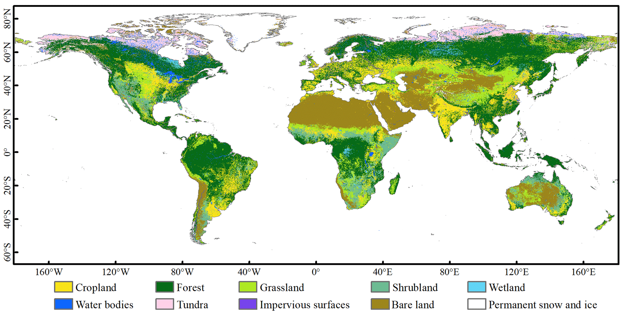
Figure 5 Global land cover map in 2015 with 30 m resolution (GLC-2015).

4.2 Accuracy assessment of the GLC-2015 map

4.2.1 Accuracy assessment with the global point-based samples

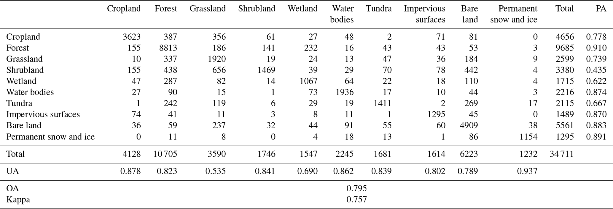
The accuracy of the GLC-2015 map was first tested via the global point-based samples, and the results of the assessment are listed in Table 3. The GLC-2015 map achieved an OA of 79.5 % and a kappa coefficient of 0.757 at the global scale, demonstrating the good performance of our map. Among all the LC classes, permanent snow and ice possessed the best mapping performance, with PA and UA achieving 89.1 % and 93.7 %. The accuracy of water bodies, forest, and impervious surfaces was also high, where PA and UA exceeded 80.0 %. Grassland, shrubland, and wetland had relatively low accuracy, with PA below 75.0 %. Among them, grassland and shrubland were mainly confused with forest, which might be because these classes are both vegetation, thus causing difficulty in recognition by spectral information. Due to the complex spectral characteristics, wetland is often mixed with vegetation (Ludwig et al., 2019).

Table 3 The confusion matrix for the GLC-2015 map based on the global point-based samples.

The regional accuracies are presented in Fig. 6. The OA of GLC-2015 ranged from 66.4 % to 93.4 % and the kappa coefficient from 0.552 to 0.813. From the perspective of OA, water regions lead, followed by tropical desert, temperate continental forest, and polar. These are areas with homogeneous land cover and low difficulty in mapping. Boreal tundra woodland, tropical dry forest, tropical shrubland, and subtropical desert are the regions with low OA. The first one may be related to the high latitudes. The following two may be because they belong to areas with complicated and mixed LC classes, which is not easily classified. The last one may be the consequence of sparse vegetation in desert areas. For the kappa coefficient, the ranking was similar to those for OA.

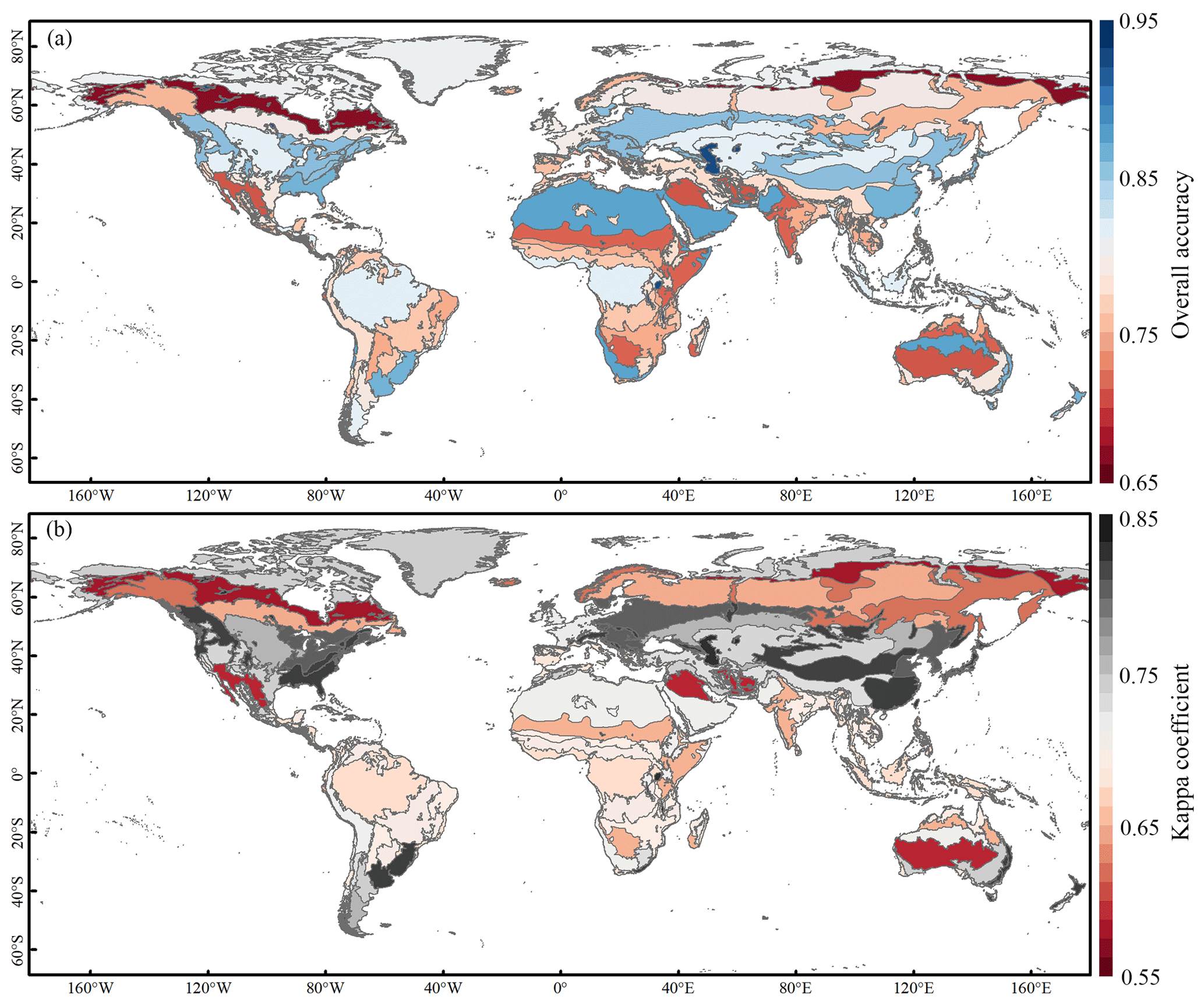
Figure 6 Regional accuracy of the GLC-2015 map according to ecoregions. (a) Overall accuracy and (b) kappa coefficient. The ecoregion boundaries are obtained from the Food and Agriculture Organization of the United Nations (FAO).

4.2.2 Accuracy assessment with the global patch-based samples

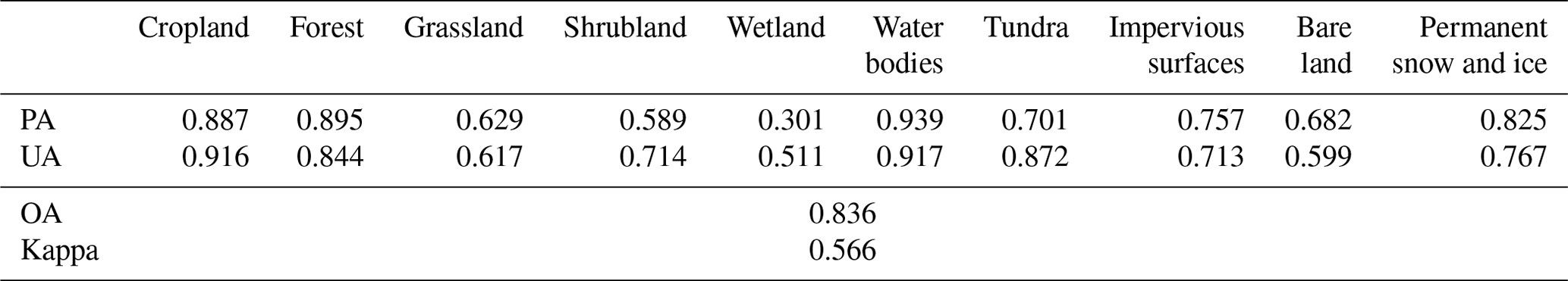
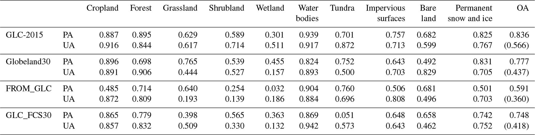
The accuracy assessment of the GLC-2015 map was also conducted with the global patch-based samples. Table 4 summarizes the results for the accuracy assessment of each LC class in the GLC-2015 map. From the assessment results, it can be found that the OA of the GLC-2015 map reached 83.6 %, which was higher than the 79.5 % tested with the global point-based samples. The kappa coefficient of the GLC-2015 map was 0.566, which was 0.191 lower than the result calculated with the global point-based samples. In both accuracy assessment results based on two different validation data sets, water bodies, forest, and permanent snow and ice were validated to have high accuracy, and grassland, shrubland, and wetland were validated to have low accuracy. Nevertheless, the ranking of accuracy for each LC class had a slight difference. For example, in assessment based on the global point-based samples, impervious surfaces and permanent snow and ice ranked higher than that based on the global patch-based samples. This may be because a LC map can easily show where one LC class is distributed but can hardly describe its actual shape. In addition to the accuracy assessment on a pixel scale, validation on a patch scale is equally important because it can reflect the shape consistency between the GLC-2015 map and the actual landscape, even if the size of global patch-based samples is relatively small. Overall, no matter the respective global point-based samples or the global patch-based samples, the mapping accuracies of the GLC-2015 map are satisfactory.

Table 4 Mapping accuracy via the global patch-based samples for the GLC-2015 map.

4.3 Intercomparison with existing GLC products

4.3.1 Intercomparison based on the global point-based samples

Based on the global point-based samples, the intercomparison of the GLC-2015 map with GlobeLand30, FROM_GLC, and GLC_FCS30 were conducted. The accuracy assessment results for all the GLC maps are listed in Table 5. It can be found that the GLC-2015 map achieved the highest OA of 79.5 % compared with GlobeLand30 of 65.3 %, FROM_GLC of 61.7 %, and GLC_FCS30 of 65.5 %, respectively. The accuracy gap between the GLC-2015 map and other existing ones was 14.0 %–17.8 %. Also, the GLC-2015 map possessed a better kappa coefficient than other products. For all classes except tundra, the GLC-2015 map outperformed the other three maps in terms of PA. For cropland, grassland, shrubland, wetland, and tundra, the GLC-2015 map also exhibited better performance regarding UA than GlobeLand30, FROM_GLC, and GLC_FCS30. Overall, for the PA or UA, the GLC-2015 map ranked first or second in nearly all LC classes, which demonstrated that the GLC-2015 map had smaller omission and commission errors against the other three products.

Table 5 Mapping accuracy of the GLC products with the global point-based samples.

Further quantitative accuracy assessments of different GLC products were performed in 4^∘ × 4^∘ grids using the global point-based samples, and box plots were produced for each product for all grids within different ecoregions, as shown in Fig. 7. It can be found that the GLC-2015 map outperformed other existing products with the best OA and kappa coefficient across different ecoregions. Also, the mean overall accuracy of the GLC-2015 map exceeded 65.0 % in all ecoregions, showing the high quality of our mapping results. It is worth noting that the GLC-2015 map showed shorter boxes except in subtropical dry forest and subtropical desert, which means the GLC-2015 map had a relatively smaller fluctuation than other ones. In subtropical desert, tropical dry forest, and boreal tundra woodland, the OA and kappa coefficient of the four products were relatively low. However, the GLC-2015 map exceeded the highest of others and greatly improved the mean OA in these regions.

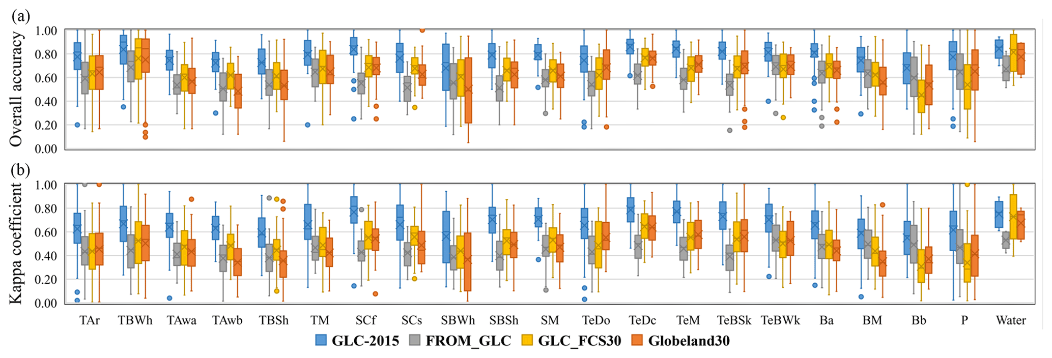
Figure 7 The box plot of the accuracy for 21 ecoregion zones. (a) Overall accuracy and (b) kappa coefficient. Ecoregion abbreviation and corresponding ecoregion are described in Table S4.

4.3.2 Intercomparison based on the global patch-based samples

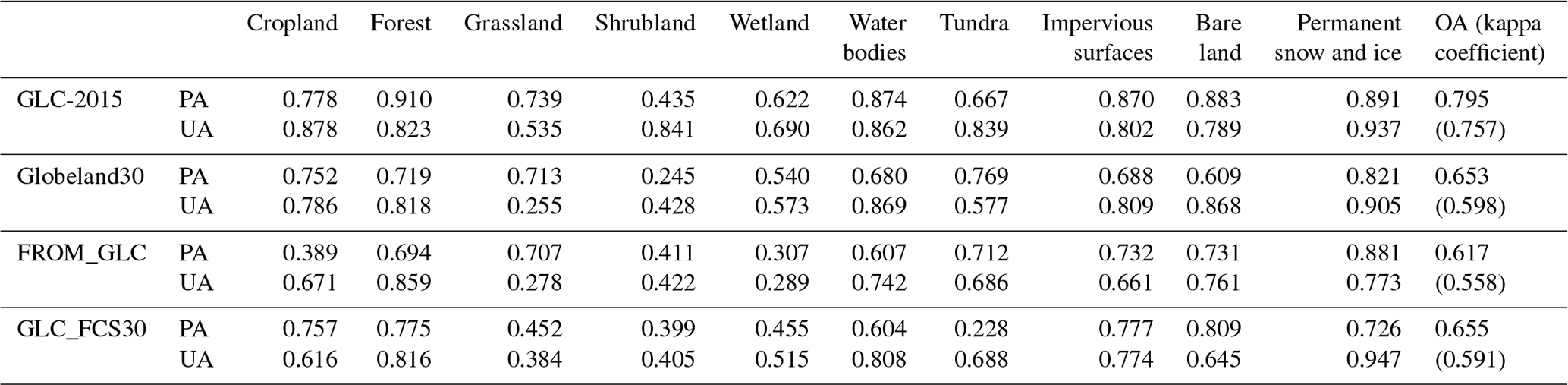
Although the global point-based samples are adequate and even across the globe, the distribution of points in each 4^∘ × 4^∘ geographical grid is too sparse to reflect the actual spatial pattern of the landscape. Focusing on the LC pattern at the local scale, we also used the global patch-based samples which can provide spatial context information to conduct the accuracy assessment of the GLC-2015 map and compare different GLC products. Table 6 lists the accuracies of the GLC-2015 map and the other three GLC products. Obviously, the GLC-2015 map achieved the best OA and kappa coefficient among these four GLC maps. The overall accuracy gap between the GLC-2015 product and others was 5.9 %–24.5 %, which presented a more significant variation compared with the result based on the global point-based samples. In terms of PA and UA, the GLC-2015 map was higher than the other three ones in most LC classes. Specifically, all the products had lower accuracy for grassland, shrubland, and wetland, similar to that in the accuracy assessment based on the global point-based samples. It is evident that FROM_GLC had the lowest mapping accuracy for grassland, shrubland, and wetland, implying that the classification method of FROM_GLC is not robust for these three LC classes.

Table 6 Mapping accuracy of the GLC products with the global patch-based samples.

Accuracy assessment was calculated in each patch-based sample, and box plots were produced for each GLC product at the continental scale, as shown in Fig. 8. The GLC-2015 map showed a robust performance in each continent, with the highest OA and kappa coefficient among all the maps. Also, in all the continents, the GLC-2015 map had the shortest boxes in terms of OA, which denoted that it had a more minor variation in accuracy at the continental scale. Among the four products, GLC_FCS30 and Globeland30 achieved similar accuracies in most continents. Obviously, FROM_GLC showed the lowest accuracy across different continents, especially in Oceania, where the OA of most patch-based samples was below 40.0 %; i.e., most of the pixels in Oceania were incorrectly classified. We further compared mapping accuracies for each LC class in different continents (Figs. S3 and S4). Since tundra and permanent snow and ice are rare and only existent in certain regions, they were not included in the comparison. As for PA across different continents, the GLC-2015 map outperformed other maps in forest, water bodies, and bare land. As for UA across different continents, the GLC-2015 map outperformed other maps in cropland, grassland, shrubland, and wetland and achieved similar accuracies to GLC_FCS30 and Globeland30 in forest. Overall, the GLC-2015 map outperformed others regarding mapping accuracy at the continental scale. In addition, all the GLC products showed significant variation and low mean accuracy in grassland, shrubland, and wetland over most continents.

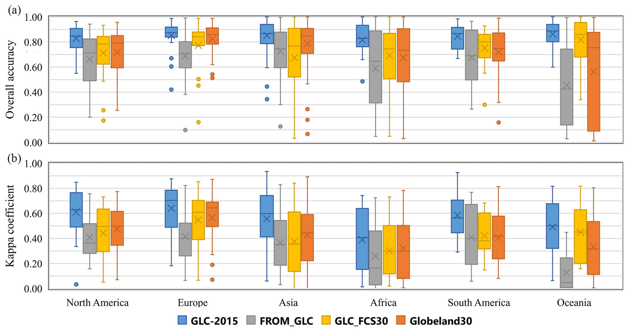
Figure 8 The box plot of the accuracy for different continents. (a) Overall accuracy and (b) kappa coefficient.

Furthermore, to compare the OA of the GLC-2015 map with other GLC products, scatter plots were used to describe the relationship between the overall accuracy of the GLC-2015 map and one other product in each patch-based sample, as displayed in Fig. 9. Most of the points were above the 1:1 line, implying that the GLC-2015 map surpassed other GLC products in terms of OA. The distribution of points was more dispersed from the 1:1 line in the plot of the GLC-2015 map against FROM_GLC compared to other plots. This indicated that these two products had a more significant difference, which was also proven in Table 6.

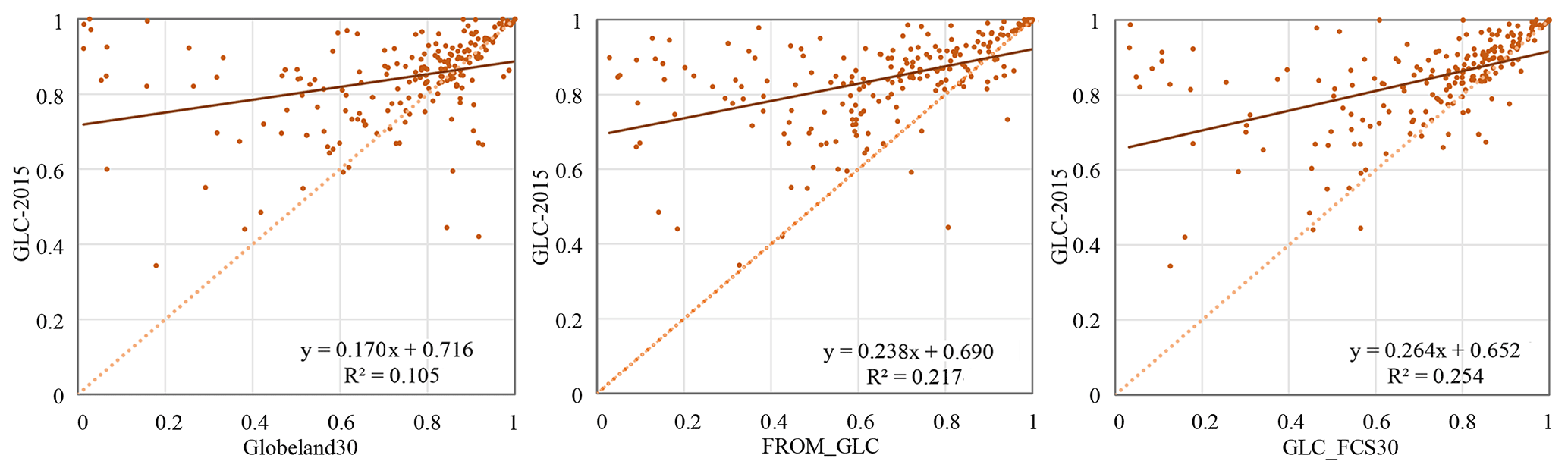
Figure 9 Scatter plots between the GLC-2015 map and other products obtained using the global patch-based samples.

4.3.3 Areal comparison for individual classes

To assess the similarities and discrepancies between GLC-2015 and other GLC products, we compared the areas of various LC classes at multiple scales, including global, continental, national, and ecoregional scales.

The areal comparison for various classes of different GLC products over the globe is shown in Fig. 10. Generally, the areas of water bodies and permanent snow and ice of four GLC products were very similar, which may be related to the similar LC definitions. In contrast, the areas of cropland, forest, grassland, and shrubland in GLC-2015 differed significantly from those in other GLC products. The area of forest in GLC-2015 is much higher than in other products. This may be because FROM_GLC and GLC_FCS30 defined forest with tree cover over 15 %, while GLC-2015 used a threshold of over 10 %. The cropland areas in GLC-2015 and Globeland30 were close, higher than FROM_GLC but lower than GLC_FCS30. Moreover, FROM_GLC underestimated the cropland area, as it had a low producer's accuracy for cropland (see Table 5), which was also demonstrated in previous studies (Liu and Xu, 2021; Zhang et al., 2021). FROM_GLC and Globeland30 shared similar grassland areas since a similar accuracy for grassland was found in these two products (see Table 5). However, FROM_GLC and Globeland30 significantly overestimated grassland extent, with much bare land misclassified as grassland (Hu et al., 2014). GLC_FCS30 showed the smallest area for grassland, which might be related to its higher threshold in vegetation cover for grassland. For shrubland, the area difference between GLC-2015 and Globeland30 was minimal, and the areas in FROM_GLC and GLC_FCS30 were similar. Furthermore, the wetland area in FROM_GLC was the lowest among all the products, with a total area of 0.168×10⁶ km². In contrast, Globeland30 and GLC_FCS30 exhibited greater wetland extent than GLC-2015 since these two products classified non-wetlands sensitive to water as wetlands (Zhang et al., 2023). In particular, the tundra area in GLC_FCS30 was much smaller than other products. This is mainly because only lichens/mosses in the original classification system of GLC_FCS30 were converted into tundra in the classification system we used, which leads to the omission of tundra. The areas of impervious surfaces in GLC-2015, Globeland30, and GLC_FCS30 were very close and higher than FROM_GLC. For bare land, there was a large difference between Globeland30 and other products, while the area in GLC-2015 and GLC_FCS30 was very close.

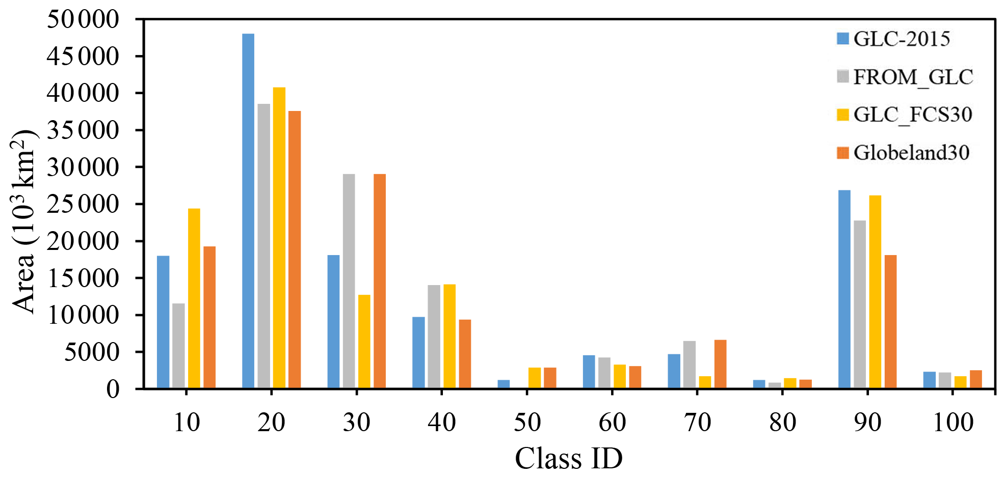
Figure 10 Areal comparison of various land cover classes among GLC products at the global scale. Class IDs 10, 20, 30, 40, 50, 60, 70, 80, 90, and 100 denote cropland, forest, grassland, shrubland, wetland, water bodies, tundra, impervious surfaces, bare land, and permanent snow and sea ice, respectively.

The area similarity and difference for various classes of different GLC products were also compared over six continents, the top 40 countries ranked by area, and 21 ecoregions (Figs. S5–S7). Overall, the four products showed a similar distribution trend of different classes. For most LC classes, the continental, national, and ecoregional rankings of the four products agreed with their ranking at the global scale, whereas, for grassland and shrubland, the area ranking of the four products varied at three different regional scales.

4.3.4 Visual intercomparison for individual classes

The visual comparison of cropland in GLC-2015, Globeland30, FROM_GLC, GLC_FCS30, Global Food Security-Support Analysis Data (GFSAD30) (Xiong et al., 2017; Teluguntla et al., 2018), and other national-scale maps was conducted in three local regions (Fig. S8). In the Egyptian agricultural area, GLC-2015, FROM_GLC, and GLC-FCS30 shared a similar delineation of the cropland and had a good representation of cropland with fine spatial details. Since the date time of the Google Earth image is 2015, Globeland30 missed the newly cultivated cropland. GFSAD30 had the largest cropland area among five products but misclassified bare land as cropland. In the agricultural area of southeastern China, GLC-2015 had agreement with GFSAD30 and CLCD. Globeland30 and GLC_FCS30 overestimated the area of cropland. As for FROM_GLC, it failed to depict the spatial distribution of cropland and had many omissions. In cropland-dominated areas of the United States, FROM_GLC significantly underestimated the extent of cropland. The other five products exhibited a similar delineation of cropland, but there were little differences in some small areas. For example, Globeland30 misclassified some grassland into cropland, and NLCD 2016 had a good ability to distinguish the farm track.

We also compared the performance in the forest of different products in three forest-prevalent regions of Congo, China, and the United States (Fig. S9). Overall, GLC-2015 and Globeland30 showed accurate delineation in three regions. FROM_GLC also had good performance for the forest in Congo and the USA but overestimated the forest in China, mislabeling shrubland and grassland as forest. Furthermore, GFC tended to miss sparse trees in China, and GLC_FCS30 underestimated the extent of forest in all three regions. As for national-scale products, CLCD and NLCD 2016 had a good ability to identify the details of forest, while CLUD dramatically missed both dense and sparse woodlands.

Furthermore, to compare the performance in the wetland of GLC-2015 with other global- and national-scale products, three wetland regions in southern–central Canada, coastal America, and Sundarbans were selected. It can be found that GLC-2015 and Globeland30 had similar representation and performed well in identifying the wetland over three regions (Fig. S10). Unexpectedly, FROM_GLC performed poorly in each region, with almost no wetlands captured. GLC_FCS30 also showed unstable quality in three regions. For example, it highly underestimated the wetland area in coastal America and completely mislabeled the mangroves as cropland in Sundarbans. NLCD 2016 and GMW accurately demonstrated the spatial pattern of the wetland, while the CA_wetlands map underestimated the wetland extent because it defined wetlands by a wetland frequency of no less than 80 % from 2000 to 2016 (Wulder et al., 2018).

To understand the spatial distribution of impervious surfaces in different products, a comparison of mapping results for three megacities, including Tokyo, Shanghai, and New York, is shown in Fig. S11. In Tokyo, a high consistency was found between GLC-2015, FROM_GLC, and GAUD, and both successfully captured the impervious surfaces in peri-urban areas. GLC_FCS30 showed the largest area for impervious surfaces because it misclassified many croplands as impervious surfaces. In Shanghai, GLC_FCS30 underestimated the central city, and CLUD lost the details of impervious surfaces because it was developed using the visual interpretation method. Other products generally had a similar representation and accurately demonstrated the spatial distribution of the city. For New York, FROM_GLC, GLC_FCS30, and GAUD agreed well with GLC-2015, while Globeland30 and NLCD 2016 had higher impervious areas than others.

4.3.5 Visual intercomparison at the local scale

We selected six typical geographical tiles covering six continents and different landscape environments to further present the mapping performance of the GLC-2015 map, Globeland30, FROM_GLC, and GLC_FCS30, as shown in Fig. 11. Overall, from a local point of view, the GLC-2015 map tended to be more diverse in LC classes and had better identification performance in various classes. In flattened cropland areas (Fig. 11a and b), the GLC-2015 map revealed diverse LC classes and accurately distinguished impervious surfaces; however, Globeland30 exaggerated the extent of impervious surfaces, and FROM_GLC failed to delineate impervious surfaces with small sizes. In addition, FROM_GLC misclassified some cropland pixels as grassland (Fig. 11a) and had an abnormal “stamp” (Fig. 11b). As for mountain areas (Fig. 11c and d), the GLC-2015 map uncovered the spatial pattern of natural and planted forest, cropland, and grassland. There were large confusions between cropland and grassland in the results of FROM_GLC and GLC_FCS30, and some impervious surfaces and cropland areas were wrongly labeled as bare land by FROM_GLC. The areas (Fig. 11c), which were classified as forest, were misidentified as cropland and grassland in three other products. For the rainforest areas where a large number of trees were reclaimed for cropland (Fig. 11e), the GLC-2015 map, Globeland30, and GLC_FCS30 had similarities in cropland areas, but FROM_GLC recognized some reclaimed areas as grassland. Additionally, the GLC-2015 map accurately presented the spatial distribution of impervious surfaces, while other products had omission or commission errors. In the cropland-dominated areas (Fig. 11f), the GLC-2015 map and Globeland30 showed a higher agreement, and both of them mapped the undulating areas as grassland. Unlike the aforementioned two products, FROM_GLC misclassified large tracts of croplands as grasslands, and GLC_FCS30 did not capture the grassland in undulating areas. Figure 11 also shows the belief measure of the fused result in different geographical tiles. Although it does not directly evaluate the mapping accuracy, it serves as a degree of support for the hypothesis of an accepted LC class being true and it can still reflect the quality of the GLC-2015 map. Overall, Bel of the GLC-2015 map exceeded 80 % in most areas of each tile, demonstrating the credibility and high quality of our mapping result.

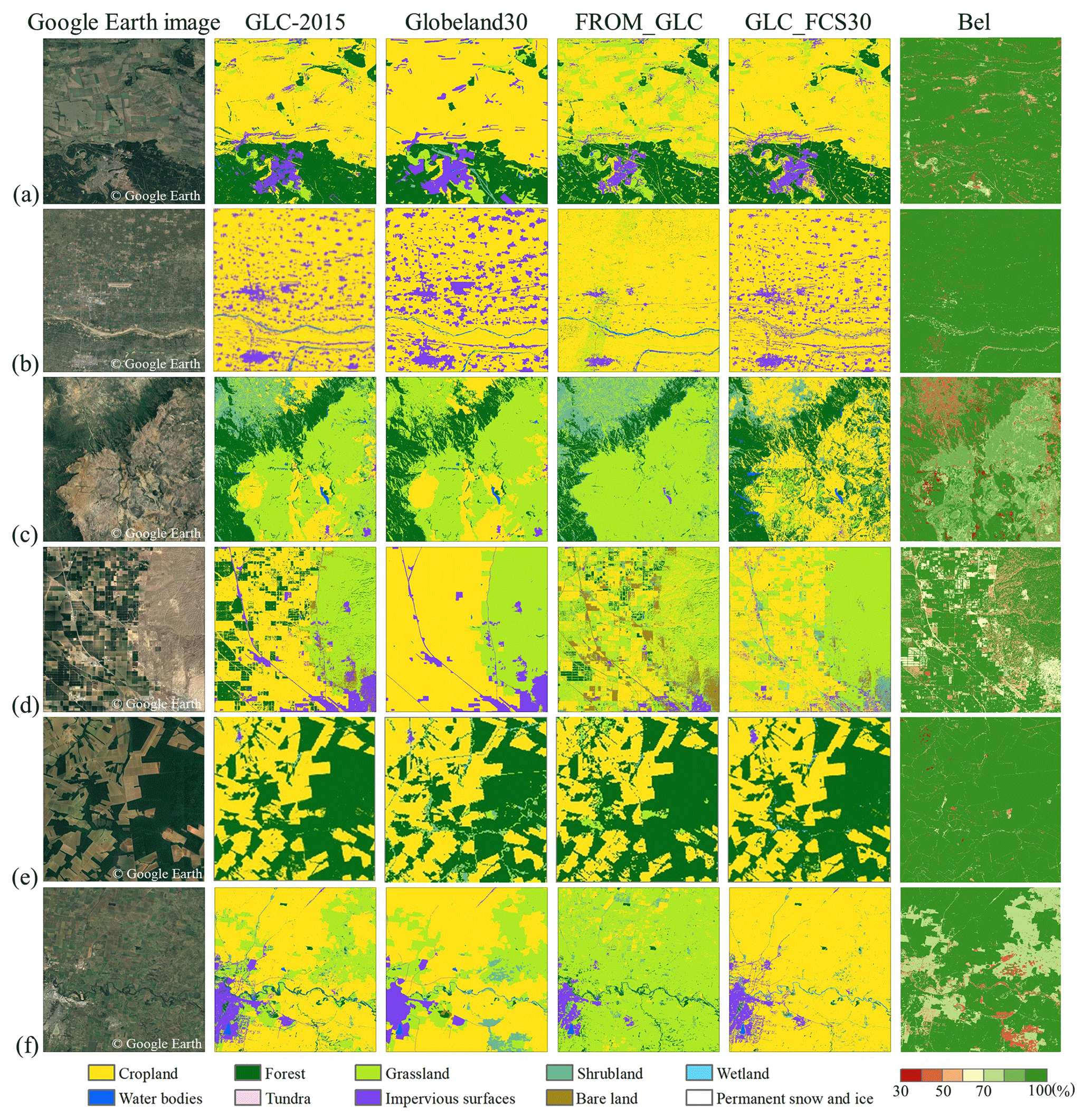
Figure 11 Visual comparison between the GLC-2015 map and three other products for different continents. Panels (a) to (f) are examples for Europe, Asia, Africa, North America, South America, and Oceania, respectively.

4.4 Intercomparison with national-scale products

Except for comparison with the existing GLC products, GLC-2015 was also compared with three national-scale products (CLCD, CLUD, and NLCD 2016 over the CONUS). We first compared the accuracy of GLC-2015 with NLCD 2016, CLCD, and CLUD using the point-based samples (Tables S5–S6). It can be found that GLC-2015 obtained an overall accuracy of 88.8 % in China, higher than CLCD (78.3 %) and CLUD (70.2 %). Specifically, GLC-2015 achieved the highest PA and UA in all LC classes except wetland and impervious surfaces. In the CONUS, GLC-2015 outperformed NLCD 2016, with an OA improvement of 13.2 %. Additionally, GLC-2015 exhibited better mapping performance in nearly all LC classes.

An accuracy comparison between GLC-2015 and three national-scale products was also performed using patch-based samples (Tables S7–S8). Overall, GLC-2015 achieved a better OA of 85.7 % in China with respect to CLCD (83.6 %) and CLUD (75.4 %). In terms of PA and UA, GLC-2015 ranked first and second in most LC classes. In the CONUS, GLC-2015 possessed an OA of 84.5 % and a kappa coefficient of 0.787, outperforming NLCD 2016. Although GLC-2015 had lower PA or UA in cropland, forest, and impervious surfaces compared to NLCD 2016, GLC-2015 outperformed NLCD 2016 in other LC classes.

We further performed an areal comparison for each LC class of GLC-2015 and three national-scale products (Figs. S12 and S13). Generally, GLC-2015, CLCD, and CLUD exhibited similar areas in most classes. Notably, the areas of cropland, shrubland, and wetland in GLC-2015 were very close to CLCD but different from CLUD. In the CONUS, the areas of cropland, water bodies, and bare land in GLC-2015 and NLCD 2016 were close. In contrast, the areas of the remaining LC classes in GLC-2015 showed a large difference from NLCD 2016. The area differences in forest, grassland, and shrubland between GLC-2015 and NLCD 2016 were mainly related to different LC definitions. For example, the minimum fraction of tree cover in the forest is 10 % in GLC-2015, whereas NLCD 2016 used a minimum fraction of 20 %. NLCD 2016 had higher areas of impervious surfaces than GLC-2015 because “open urban” in NLCD 2016 includes too much vegetation.

4.5 Improvement of the GLC-2015 map compared to existing GLC products

The spatial distribution of inconsistency between three GLC products at the global scale is illustrated in Fig. 12. From the inconsistency map, we found that areas of low inconsistency mainly corresponded to homogeneous regions with simple LC classes. For example, the northern part of Africa was mainly classified as bare land, the northern part of South America was mainly classified as forest, and Greenland was classified as permanent snow and ice. By contrast, areas of high inconsistency were located in regions with complicated LC classes, especially in mixed-vegetation regions or sparse-vegetation regions, such as northern Asia, southern Africa, the Sahel region, Australia, northern and southern North America, and eastern and southern South America.

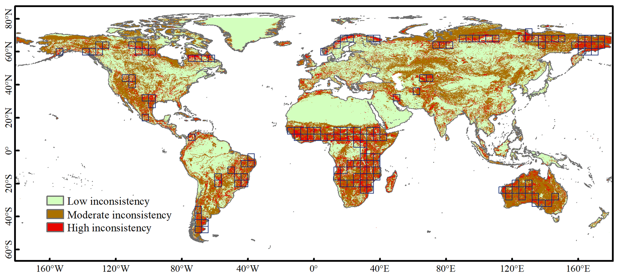
Figure 12 Distribution of inconsistency between Globeland30, FROM_GLC, and GLC_FCS30. The blue rectangles are high-inconsistency grids where the areas of pixels with a value equal to 1 account for more than 20 % of the total area.

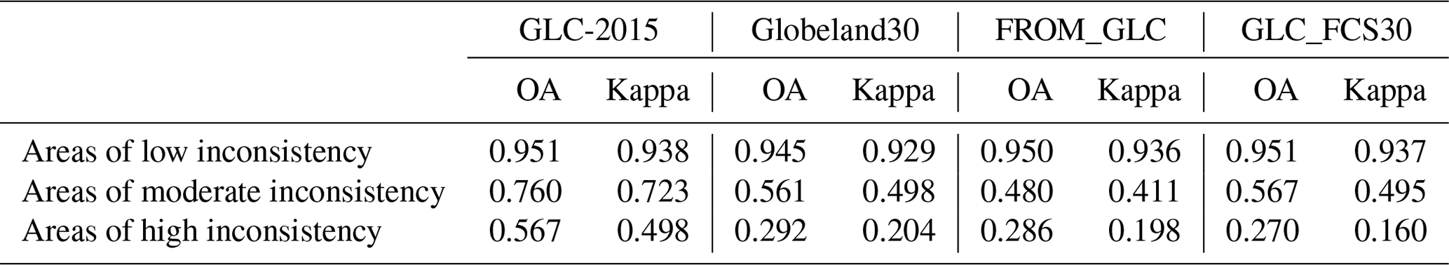
Based on the global point-based samples, we assessed the accuracies of the GLC-2015 map, Globeland30, FROM_GLC, and GLC_FCS30 in the aforementioned areas of low inconsistency, moderate inconsistency, and high inconsistency, as shown in Table 7. Overall, the GLC-2015 map had the highest accuracies against the other three ones in three areas. For each product, areas of low inconsistency obtained the highest accuracies, followed by areas of moderate inconsistency and then high inconsistency, which demonstrated that inconsistency of the existing products could indicate the quality of maps. In areas of low inconsistency, the overall accuracy gap between the GLC-2015 map and previous ones was as small as 0.1 %–0.6 %. However, for areas of moderate and high inconsistency, the comparison accuracy gap expanded to 19.3 %–28.0 % and 27.5 %–29.7 %, respectively. It proved the outperformance of the GLC-2015 map over the other three products in the areas of high identification difficulty.

Table 7 Accuracy assessments of the GLC products in three areas.

We further provided a comparative analysis of three previous GLC products and the GLC-2015 map in areas of high inconsistency. We calculated the area of pixels with a value equal to 1 in 4^∘ × 4^∘ grids. The grids where the areas of pixels with a value equal to 1 account for more than 20 % of the total area were selected as grids of high inconsistency. Finally, a total number of 147 grids were selected (Fig. 12). To compare the accuracy of the GLC-2015 map and other ones, we utilized scatter plots to represent the relationship between the overall accuracy of one previous product and the GLC-2015 map in each grid of high inconsistency based on the global point-based samples (Fig. 13). Most of the points were above the 1:1 line; i.e., the values of y axes corresponding to those points were larger than the values of x axes, which demonstrated that the GLC-2015 map performed better than other GLC products in most grids of high inconsistency. It can be found that the fitting line in each scatter plot had an intercept exceeding 0.40, a slope less than 0.55, and R² less than 0.35, showing that the GLC-2015 map had a large difference from other ones.

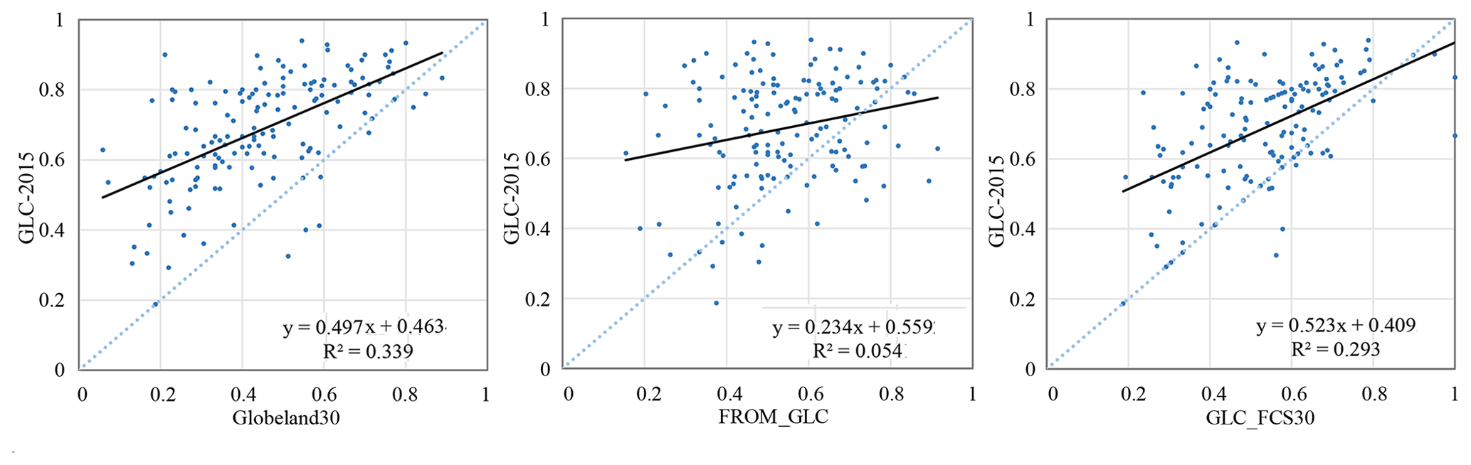
Figure 13 Overall accuracy relationship between the GLC-2015 map and other products in grids of high inconsistency.

To intuitively compare the mapping result of the GLC-2015 map and three existing ones in areas of high inconsistency, we focused on visual inspection in various areas based on four 5 km × 5 km patch-based samples and conducted accuracy statistics as shown in Fig. 14. In the detailed display, it is apparent that three previous products had a large difference in four areas. As can be seen from the four visual cases, the typical confusions between LC classes in areas of high inconsistency were as follows. (1) Shrubland was easily misclassified as forest and grassland. (2) Cropland, grassland, and shrubland were heavily confused with each other. (3) Bare land was likely to be mixed with shrubland and grassland. Overall, the GLC-2015 map surpassed other products in the local accuracy assessment. In western Australian mulga shrublands (Fig. 14a), the GLC-2015 map and GLC_FCS30 showed a similar spatial distribution and shape of bare land and forest, which was consistent with the real landscape, while Globeland30 classified bare land as grassland and FROM_GLC underclassified bare land. As for Zambezian and mopane woodlands (Fig. 14b), the GLC-2015 map performed best, with OA reaching 82.6 %, followed by FROM_GLC. In contrast, other products mixed shrubland with forest or grassland. In agricultural land of the western United States (Fig. 14c), GLC-2015 and Globeland30 exhibited similar mapping results to the ground truth, while FROM_GLC had a large difference from other products. When it comes to the Guinean forest–savanna mosaic (Fig. 14d), the GLC-2015 map and Globeland30 showed high spatial consistency, and both had an accurate classification profile for cropland, forest, and impervious surfaces, while other products misidentified cropland as other LC classes.

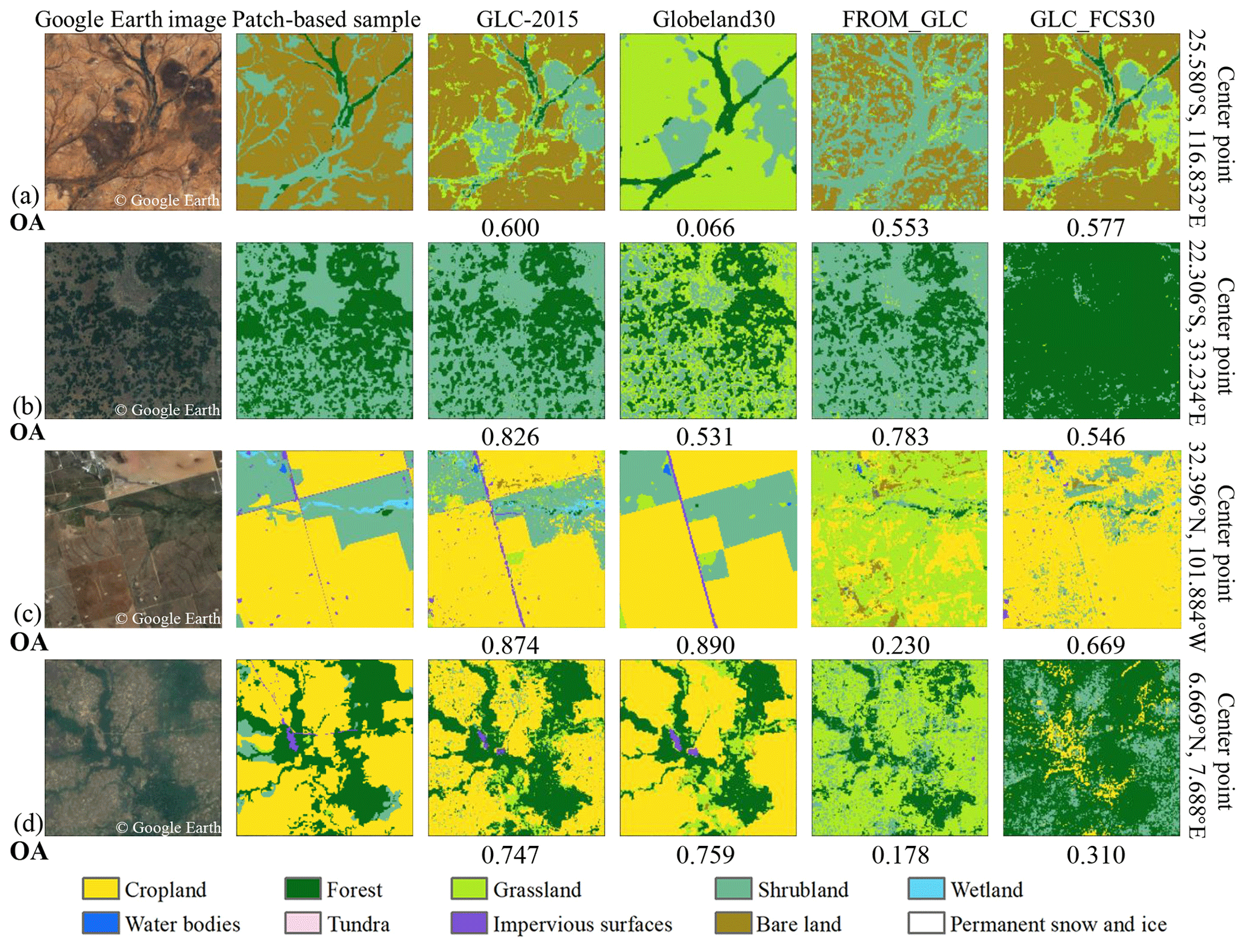
Figure 14 Visual comparison between the GLC-2015 map and three other products based on 5 km × 5 km patch-based samples and Google Earth images for four areas of high inconsistency (a–d). The OA for each product was calculated by the corresponding patch-based sample.

4.6 Comparison between DSET and other methods

4.6.1 Intercomparison with other data-fusion methods

The accuracy assessments of GLC-2015 obtained by the DSET and global mapping results from two other data-fusion methods were conducted based on two global validation sample sets. The confusion matrices with the global point-based samples are shown in Tables S9 and S10. The OA of the global land cover classification obtained by the MV and SC was 72.1 % and 71.8 %, respectively. As shown in Table 3, the OA of the GLC-2015 map obtained by the DSET method was 79.5 %, which had an improvement of 7.4 % and 7.7 % compared to mapping results from the MV and SC. In addition, the GLC-2015 map obtained higher PA and UA for most LC classes.

When evaluating GLC maps obtained by different data-fusion approaches using the global patch-based samples, the DSET method obtained the highest OA of 83.6 % and a kappa coefficient of 0.566, compared with 80.1 % and 0.497 for MV and 71.8 % and 0.391 for SC (Table S11). Here, the DSET method achieved an accuracy improvement of 3.5 % and 11.8 %. Compared to the other two methods, the DSET improved the accuracy for nearly all the LC classes, especially for grassland, shrubland, and wetland. We also compared the overall accuracy relationship between the DSET and other methods. From the scatter plots (Fig. 15), we found that the majority of points were above the 1:1 line, implying that the DSET had better mapping performance than others in most regions across the globe.

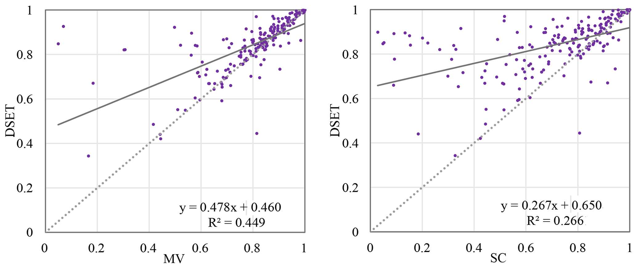
Figure 15 Scatter plots between the DSET and other data-fusion methods based on the global patch-based samples.

Land cover mapping results from the DSET and other methods were also visually illustrated in six tiles with a size of 0.25^∘ covering different continents, as displayed in Fig. S14. Despite mapping results from the DSET and MV depicting similar spatial distributions of LC classes in all tiles except the tile in North America, the DSET more accurately delineated the impervious surfaces of small sizes which scattered in cropland-dominated (Fig. S14a) or arid (Fig. S14c) areas. Notably, the mapping results from the SC method presented significant differences from those obtained by the DSET and MV. For example, the SC method failed to capture scattered rural residential areas (Fig. S14b) and misclassified grassland as cropland (Fig. S14d). Overall, the DSET method possessed better recognition performance in various LC classes than the other two methods.

4.6.2 Intercomparison with the random forest

Based on the validation data from 20 % of the global point-based samples, we evaluated the quality of the GLC-2015 map obtained by the DSET method and mapping results classified by the RF classifier for a total of 300 grids. The DSET method obtained a mean OA of 80.9 % across six continents, while the RF achieved a lower accuracy of 69.9 %. From the scatter plots which compared the OA and kappa coefficient between the DSET and RF grid by grid, it was found that the DSET possessed higher accuracy in most grids (Fig. S15). In particular, the points were clustered in the upper-right corner of the plot (Fig. S15a), which indicated that the RF classifier trained with the global point-based samples performed well in those selected grids, though it was inferior to the DSET method. Figure S16 shows the OA of the DSET and RF across six continents. We found that the DSET method outperformed the RF classifier for each continent. In particular, the mapping results of both methods presented the lowest accuracy in Oceania. This may be because the selected grids are located in regions with a heterogeneous landscape. As for the box plot for the RF classifier, the low hinge exceeded 60.00 % in all continents except Oceania, demonstrating the reliability of the RF classifier trained by the global point-based samples. Nevertheless, the performance of the RF classifier was worse than the DSET method. This highlights the feasibility of the DSET method in integrating the existing maps for a better one.

4.7 Advancement and limitations

To address the problem where current 30 m GLC products have great inconsistency in heterogeneous areas and low mapping accuracy for spectral similar LC classes, this study adopted a multisource product-fusion approach based on the DSET to create an improved global land cover map (GLC-2015). The results show that GLC-2015 had good mapping performance, with OA reaching 79.5 % and 83.6 % based on two different validation sets. Compared with those existing products, GLC-2015 greatly improved the accuracy across the globe, especially in areas of high inconsistency with a significant improvement of 27.5 %–29.7 %. Compared with other commonly used data-fusion methods, the adopted DSET approach provided a higher OA and kappa coefficient which showed the benefit of the DEST in integrating various land cover data. No matter the respective global point-based samples or the global patch-based samples, GLC-2015 showed relatively low accuracy for grassland, shrubland, and wetland compared to other LC classes. Those LC classes are challenging to map at the global scale due to their spectral similarity to other classes, ambiguous definitions, or variety with regions. However, compared to other existing 30 m GLC products, the GLC-2015 map performed better with the PA and OA ranking first or second for grassland, shrubland, and wetland, which indicated the improvement of GLC-2015 in poorly mapped LC classes. It was found that the GLC-2015 map had worse performance in areas with more disagreements (Table 7). However, the GLC-2015 map surpassed other products, particularly in highly inconsistent areas. Moreover, the accuracy gap between the GLC-2015 map and other ones in areas of high inconsistency was larger than that in areas with fewer disagreements, implying that the GLC-2015 map provides a more accurate characterization of land cover in poorly mapped areas. Although the GLC-2015 map was not capable of avoiding all the wrong mapping results caused by the disagreements from the candidate GLC products, it outperformed the existing products from the aspects of mapping accuracy for the easily misclassified classes and areas with great inconsistency.

Although the GLC-2015 map can evidently improve mapping accuracy in inconsistent areas, there are still some uncertainties. First, we used three multiple-class GLC maps and four single-class GLC maps as the source data for integration. Since those products provided information on land cover at the global scale, classification errors inevitably exist in some specific regions. The multisource product-fusion method based on the DEST depends highly on the quality of those candidate maps, such that the inconsistency between those source maps might lead to incorrect classification. Second, the date time of GlobeLand30 is different from that of other maps. Because of the 5-year time interval, there are changes in land cover, which inevitably distort the fusion results. However, the changed areas are tiny compared to the world's terrestrial area. The uncertainties caused by the LC changes are minor compared with those from classification errors. In addition, the global point-based samples were used to evaluate the reliability of each product. The accuracy of GlobeLand30 was lower than the other products for areas with LC changes. In this case, the fusion depended more on other maps to avoid the errors caused by LC changes. Third, due to the different LC definitions, uncertainties in classification system conversion are inevitable (Zhang et al., 2017), which might cause problems for the fusion based on the DSET method. However, we conducted a reliability evaluation of the candidate maps to reduce the influence of uncertainties in classification system conversion on the fusion. The point-based samples used for reliability evaluation were labeled referring to the LC definitions in our classification system, so that all the maps were evaluated under the criterion of the classification system we used. By the reliability evaluation, the candidate maps were assessed to have lower accuracy for areas with mismatched information. When integrating all the maps grid by grid, the mismatched information would contribute less to the fusion. Lastly, most candidate LC products used a simple classification system without a level-2 classification system, so they made no contributions to a more detailed classification system when they served as source data for data fusion. Although some maps provided detailed LC classification results, such as GLC_FCS30 and FROM_GLC for 2015, there might be several challenges in the standardization and uniformity of level-2 classification systems due to the large discrepancies in the definition and criteria. Therefore, GLC-2015 adopted a simple classification system containing 10 major LC classes. In future work, measures will be taken to meet the expectation of a more detailed classification system for GLC mapping. An improved GLC product with a detailed classification system rather than a simple one-level classification system can be further developed based on the highly applicable and general DSET method whenever more products with diverse LC classes are available. Additionally, a feasible framework for the conversion of different level-2 classification systems into a uniform system should be developed.

5 Data availability

The improved global land cover map in 2015 with 30 m resolution is available at https://doi.org/10.6084/m9.figshare.22358143.v2 (Li et al., 2023). The GLC-2015 product is organized by a total of 1507 4^∘ × 4^∘ geographical grids in GeoTIFF format across the world's terrestrial area. Each image of the GLC-2015 product is named “GLC-2015_long_lat” (long and lat represent the longitude and latitude of the grid's lower-left corner, respectively).

6 Conclusions

GLC information at fine spatial resolution is vital for the global environment and climate studies which can capture the footprint of human activity. Resulting from the differences in the classification scheme, satellite sensor data, classification algorithms, and sampling strategies, the existing GLC products have high inconsistency in some parts of the world, especially in fragmented areas and transition zones. More accurate and reliable data with accuracy improved in areas of high mapping inconsistency are very desirable. In this study, with the help of the GEE platform, we developed the GLC-2015 map by integrating multiple existing GLC maps based on the DSET. The GLC-2015 map can significantly increase the mapping accuracy and possess good recognition performance in various LC classes.

The GLC-2015 map was validated by both the global point-based samples and the global patch-based samples. Accuracy assessments show that the GLC-2015 map achieved an OA of 79.5 %, a kappa coefficient of 0.757 using a total of 34 711 global point-based samples, an OA of 83.6 %, and a kappa coefficient of 0.566 using a total of 201 global patch-based samples. Data intercomparison indicated that the GLC-2015 map surpassed three other products both visually and quantitatively by OA improvement of 14.0 %–17.8 % validated with the global point-based samples and 5.9 %–24.5 % with the global patch-based samples. Compared to other products, there are fewer misclassifications in the GLC-2015 map for most LC classes, such as forest, cropland, shrubland, and water bodies. Meanwhile, the GLC-2015 map outperformed others in terms of OA and kappa coefficient across different ecoregions and different continents. Notably, the GLC-2015 map showed better performance than others by an increment of 0.1 %–0.6 % in overall accuracy for areas of low inconsistency, 19.3 %–28.0 % for areas of moderate inconsistency, and 27.5 %–29.7 % for areas of high inconsistency. In addition, the mapping results obtained by the DSET surpassed other data-fusion methods, with OA improvement of 7.4 %–7.7 % via the global point-based samples and 3.5 %–11.8 % via the global patch-based samples. Therefore, it can be concluded that the GLC-2015 map is a robust and reliable map that can significantly improve mapping accuracy compared to previous GLC products and mapping results from other common data-fusion methods.