Spatial reconstruction of long-term (2003–2020) sea surface pCO₂ in the South China Sea using a machine-learning-based regression method aided by empirical orthogonal function analysis

The South China Sea (SCS) is the largest marginal sea of the North Pacific Ocean, where intensive field observations, including mappings of the sea surface partial pressure of CO₂ (pCO₂), have been conducted over the last 2 decades. It is one of the most studied marginal seas in terms of carbon cycling and could thus be a model system for marginal sea carbon research. However, the cruise-based sea surface pCO₂ datasets are still temporally and spatially sparse. Using a machine-learning-based method facilitated by empirical orthogonal function (EOF) analysis, this study provides a reconstructed dataset of the monthly sea surface pCO₂ in the SCS with a reasonably high spatial resolution (0.05^∘ × 0.05^∘) and temporal coverage between 2003 and 2020. The data input to our model includes remote-sensing-derived sea surface salinity, sea surface temperature, and chlorophyll, the spatial pattern of pCO₂ constrained by EOF, atmospheric pCO₂, and time labels (month). We validated our reconstruction with three independent testing datasets that are not involved in the model training. Among them, Test 1 includes 10 % of our in situ data, Test 2 contains four independent in situ datasets corresponding to the four seasons, and Test 3 is an in situ monthly dataset available from 2003–2019 at the South East Asia Time-series Study (SEATs) station located in the northern basin of the SCS. Our Test 1 validation demonstrated that the reconstructed pCO₂ field successfully simulated the spatial and temporal patterns of sea surface pCO₂ observations. The root mean square error (RMSE) between our reconstructed data and in situ data in Test 1 averaged ∼10 µatm, which is much smaller (by ∼50 %) than that between the remote-sensing-derived data and in situ data. Test 2 verified the accuracy of our retrieval algorithm in months lacking observations, showing a relatively small bias (RMSE of ∼8 µatm). Test 3 evaluated the accuracy of the reconstructed long-term trend, showing that, at the SEATs station, the difference between the reconstructed pCO₂ and in situ data ranged from −10 to 4 µatm (−2.5 % to 1 %). In addition to the typical machine learning performance metrics, we assessed the uncertainty resulting from reconstruction bias and its feature sensitivity. These validations and uncertainty analyses strongly suggest that our reconstruction effectively captures the main spatial and temporal features of sea surface pCO₂ distributions in the SCS. Using the reconstructed dataset, we show the long-term trends of sea surface pCO₂ in five subregions of the SCS with differing physicobiogeochemical characteristics. We show that mesoscale processes such as the Pearl River plume and China coastal currents significantly impact sea surface pCO₂ in the SCS during different seasons. While the SCS is overall a weak source of atmospheric CO₂, the northern SCS acts as a sink, showing a trend of increasing strength over the past 2 decades. The data used in this article are available at https://doi.org/10.57760/sciencedb.02050 (Wang and Dai, 2022).

1 Introduction

The ocean possesses a large portion of the global capacity for atmospheric carbon dioxide (CO₂) sequestration, annually mitigating 22 %–26 % of the anthropogenic CO₂ emissions associated with fossil fuel burning and land use changes over the period from 2012–2021 (Friedlingstein et al., 2022). Ocean margins are an essential part of the land–ocean continuum, representing a particularly challenging regime to study (e.g., Chen and Borges, 2009; Dai et al., 2022; Laruelle et al., 2015), as they are often characterized by large spatial and temporal variations in air–sea CO₂ fluxes that lead to larger uncertainties in their overall estimation and predictions than those made in the open ocean (Dai et al., 2013, 2022; Cao et al., 2020; Laruelle et al., 2015; Chen and Borges, 2009, and references therein). Limited spatiotemporal coverage of in situ observations is a large source of these uncertainties.

In recent years, many studies have used numerical models or data-based approaches to improve estimates of the partial pressure of carbon dioxide (pCO₂) at the sea surface and the accuracy of the global carbon budget for periods and regions with poor coverage of in situ data (e.g., Rödenbeck et al., 2015; Wanninkhof et al., 2013). Numerical models can successfully quantify the generally increasing trend in oceanic pCO₂ and simulate some critical carbon cycling processes (e.g., net ecosystem production) but still suffer from regional and seasonal differences in their estimates of ocean carbonate parameters (e.g., Luo et al., 2015; Mongwe et al., 2016; Tahata et al., 2015; Wanninkhof et al., 2013). Thus, data-based approaches, which typically apply statistical interpolation and regression methods, have become an important complement to numerical models (e.g., Jones et al., 2014; Lefèvre et al., 2005; Landschützer et al., 2014, 2017; Telszewski et al., 2009). Statistical interpolation improves the spatial coverage of in situ data but does not work for periods in which in situ data are unavailable. Regression methods allow the mapping of the relationships between in situ pCO₂ data and other parameters that may drive changes in surface ocean pCO₂, and then the extrapolation of this relationship to improve estimates of the spatiotemporal distribution of pCO₂. Machine learning methods, and remote-sensing-derived products (as proxy variables in regression methods) have aided the development of data-based methods (Rödenbeck et al., 2015; Bakker et al., 2016) and can improve the model results for the oceanic carbonate system by numerical assimilation methods. Consequently, machine learning has increasingly become a routine approach for reconstructing sea surface pCO₂ in open-ocean regimes (e.g., Zeng et al., 2017; Li et al., 2019); however, it remains challenging to extend this method to ocean margins, which are more dynamic in both time and space.

The South China Sea (SCS) is the largest marginal sea of the North Pacific Ocean, with a surface area of 3.5×10⁶ km². Although extensive field observations of sea surface pCO₂ have been conducted in the SCS over the past 2 decades, their spatial and temporal coverage is still limited with respect to coverage of different physicobiogeochemical domains and subseasonal timescales (e.g., Guo and Wong, 2015; Li et al., 2020; Zhai et al., 2005, 2013). Therefore, there is a strong need for improved surface water pCO₂ coverage in the SCS to constrain air–sea CO₂ fluxes and improve initial conditions of numerical models. Moreover, the reasonably high spatiotemporal resolution of pCO₂ data can help identify the controlling factors of pCO₂ changes in the SCS and reliably resolve long-term changes.

Zhu et al. (2009) presented an empirical approach to estimate sea surface pCO₂ in the northern SCS using remote-sensing-derived (RS-derived) data, including sea surface temperature (SST) and chlorophyll a (Chl a). Their reconstructed pCO₂ data were generally consistent with the in situ data. However, uncertainties remained large, primarily caused by limited in situ data from only two summer cruises in their study. Jo et al. (2012) developed a neural-network-based algorithm using SST and Chl a to estimate sea surface pCO₂ in the northern SCS. In their study, in situ sea surface pCO₂ data were collected from three cruises during May 2001 and February and July 2004. The reconstruction also suffered a relatively large bias (Wang et al., 2021). Bai et al. (2015) employed a mechanic semi-analytical algorithm (MeSAA) to estimate satellite remote-sensing-derived sea surface pCO₂ in the East China Sea from 2000–2014 and then expanded the application of this algorithm to estimate sea surface pCO₂ for the whole China seas region, including the South China Sea. These authors explained that their MeSAA did not fully account for some localized processes, which resulted in a RMSE of about 45 µatm for the SCS (Wang et al., 2021). Yu et al. (2022) subsequently used a nonlinear regression method to develop a retrieval algorithm for seawater pCO₂ in the China seas, and the RS-derived pCO₂ data from 2003–2018 were provided by the SatCO₂ platform (http://www.SatCO2.com, last access: 8 October 2022). In this retrieval algorithm, the input parameters included sea surface temperature, Chl a concentrations, remote sensing reflectance at three bands (Rrs412, 443, and 488 nm), the temperature anomaly in the longitudinal direction, and the theoretical thermodynamic background pCO₂ under the corresponding SST. Although the RMSE associated with the RS-derived pCO₂ product was relatively large (21.1 µatm), it successfully showed the major spatial patterns of sea surface pCO₂ in the China seas (Yu et al., 2022).

To take advantage of both the high spatiotemporal resolution of the RS-derived pCO₂ data and the accuracy of the in situ data, Wang et al. (2021) reconstructed a basin-scale sea surface pCO₂ dataset in the SCS during summer using an empirical orthogonal function (EOF) based on a multilinear regression method. They demonstrated that the spatial modes of RS-derived data calculated using the EOF can effectively provide spatial constraints on the data reconstruction, and thus, this approach is adopted in this study. However, the reconstructed results may still be subject to bias when the standard deviation of spatial in situ data is relatively large because of the influence of outliers (Wang et al., 2021). Therefore, many studies have used machine-learning-based regression methods to reduce the influence of outliers in open-ocean areas and have achieved a RMSE of <17 µatm in most cases (e.g., Zeng et al., 2017; Li et al., 2019).

Building on the ability of the EOF method to significantly improve reconstructions in terms of spatial patterns and accuracy (Wang et al., 2021), we developed a machine-learning-based regression method facilitated by the EOF to fully resolve the long-term spatial distribution of sea surface pCO₂ at a resolution of 0.05^∘ × 0.05^∘ in the SCS. Our reconstructed model uses input data that include remote-sensing-derived sea surface salinity, sea surface temperature, and Chl a, the spatial pattern of pCO₂ constrained by the EOF, atmospheric pCO₂, and time labels (month). In addition to assessing typical machine learning performance metrics, we evaluated the uncertainty resulting from the bias of the reconstruction and its sensitivity to the features.

2 Study site and data sources

2.1 Study area

The SCS, located in the northwestern Pacific, is a semi-enclosed marginal sea with a maximum water depth of ca. 4700 m (e.g., Gan et al., 2006, 2010). The rhombus-shaped deep-water basin, with a southwesterly–northeasterly direction, accounts for about half of the total area of the SCS (Fig. 1). Largely modulated by the Asian monsoon and topography, the SCS exhibits seasonally varying surface circulation, river inputs, and upwelling. The circulation of the upper layer shows a large cyclonic circulation structure in winter (Fig. 1), while in summer it exhibits an anticyclonic circulation structure (Fig. 1; Hu et al., 2010). In the northern SCS, the Pearl River discharges into the SCS with an annual freshwater input of 3.26×10¹¹ m³ (e.g., Dong et al., 2004; Dai et al., 2014). The area influenced by the Pearl River plume may extend southeastward to a few hundred kilometers from the estuary in summer because of the monsoonal wind stress (Dai et al., 2014). The northern and western coastal regions of the SCS feature summer coastal upwelling, such as the eastern Guangdong and Qiongdong upwelling systems in the northern SCS and the Vietnam upwelling systems in the western SCS (e.g., Cao et al., 2011; Chen et al., 2012; Gan et al., 2006, 2010; Li et al., 2020). These seasonal changes in sea surface circulation lead to strong seasonal characteristics of sea surface pCO₂ in the SCS.

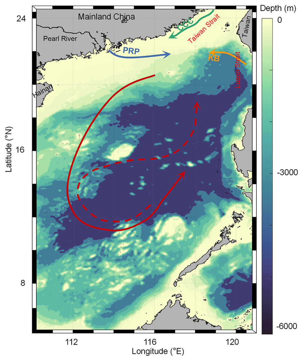
Figure 1 Topographic map of the South China Sea (SCS) showing the basin-wide cyclonic circulation in winter (solid line) and anticyclonic circulation over the southern half of the SCS in summer (dashed line). Also shown are the Kuroshio branch (KB; orange line), the China coastal current (CCC; green line), and the Pearl River plume (PRP; blue line).

The SCS is subject to dynamic water exchanges with the East China Sea via the Taiwan Strait and the western Pacific via the Luzon Strait (Fig. 1). In winter, driven by the winter monsoon, the China coastal current (CCC; green line in Fig. 1; Han et al., 2013; Yang et al., 2021) flows south along the Chinese mainland through the Taiwan Strait, and occupies the northern SCS with cold, fresh, nutrient-rich waters. The strong northeasterly winds in winter also slow down the western boundary ocean current, forcing the intrusion of Kuroshio water, featuring high surface salinity and high total alkalinity, into the SCS via the Luzon Strait (orange line in Fig. 1; Du et al., 2013; Park, 2013; Yang et al., 2021). These water exchange processes increase the complexity of the spatial distribution of sea surface pCO₂ in the SCS, which, as a result, has strong seasonal characteristics and spatial variability.

2.2 Observational pCO₂ data

Data collected from field surveys during the study period 2003–2020 are summarized in Table 1. Most observations were made in July, with fewer observations made in March and December of each year. The rough sea state in the SCS in winter and early spring limited the field surveys during these seasons. Data collected from July 2000 to January 2018 were originally published in Li et al. (2020). The in situ pCO₂ were collected from R/Vs Dongfanghong-2 and Tan Kah Kee (TKK) (shown in Table 1). During the cruises, sea surface pCO₂ was measured during the cruise. The measurements and data processing followed the SOCAT (Surface Ocean CO₂ Atlas) protocol (Li et al., 2020). More details of the data collection methods are provided in Li et al. (2020). The spatial coverage and frequency of the observations are shown in Fig. 2, revealing pronounced seasonal changes across a large spatial area. For example, the spatial coverage of the in situ data in spring and fall are relatively uniformly distributed, and the south end of the spatial coverage reaches 5^∘ N in spring, whereas during other seasons the data are concentrated in the northern and central regions of the SCS. In addition, only one observation was made in the basin area in winter, while the northern coastal area was more frequently surveyed, especially in summer.

Table 1 Summary of seasonal in situ data of sea surface pCO₂ in the South China Sea for the period 2003–2020 used in this study.

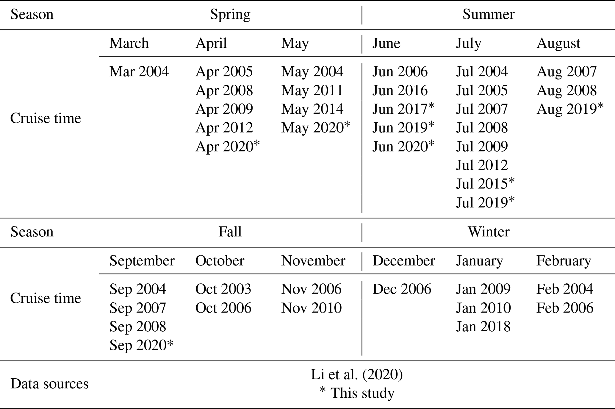
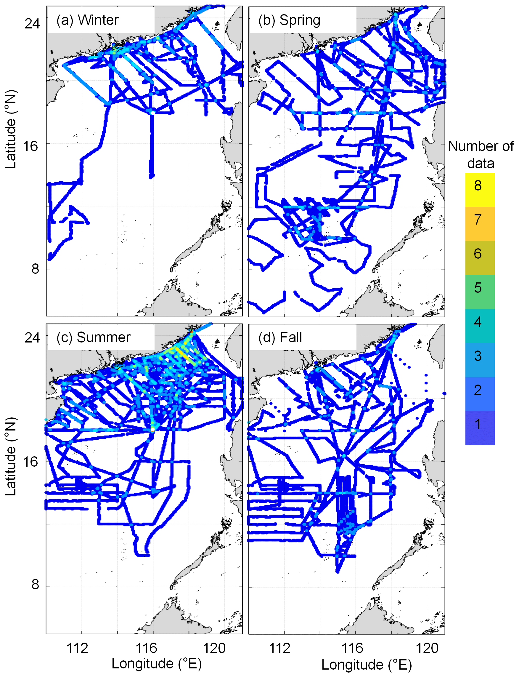
Figure 2 Cruise tracks of the observations conducted in the South China Sea in each season from 2000 to 2020. (a) Winter, (b) spring, (c) summer, and (d) fall are shown. The data collected before February 2018 are from Li et al. (2020), except for those collected in July 2015 and June 2017.

Figure 3 shows the spatial and temporal distributions of in situ sea surface pCO₂. Seasonally, the lowest pCO₂ occurs in January, and the highest concentrations occur in May and June. Spatially, the pCO₂ distribution in the basin is relatively homogeneous, although is highly variable in the northern region. In the northern coastal area in summer, the pCO₂ distribution is affected by the Pearl River plume (yielding low values) and coastal upwelling (yielding high values), which last into early fall. In winter and early spring, relatively low pCO₂ values (∼350 µatm) were found in the near-shore area. In addition, the high pCO₂ values recorded on the western side of the Luzon Strait in December demonstrate the influence of winter upwelling during some of the surveys.

In addition to the above in situ sea surface pCO₂ data, we selected in situ sea surface pCO₂ data collected during four independent surveys across the four seasons in September 2018 (fall), December 2018 (winter), August 2019 (summer), and April 2020 (spring) to verify the accuracy of our reconstruction model in extrapolating periods lacking training datasets. Furthermore, we used an additional dataset of sea surface pCO₂ calculated from observed dissolved inorganic carbon and total alkalinity during 2003–2019 at the Southeast Asia Time-series Study (SEATs) station (data from Dai et al., 2022) to test the long-term consistency of the reconstruction.

Figure 3 Seasonal and monthly sea surface pCO₂ fields in the South China Sea. (a) Winter. (b) December, (c) January. (d) February. (e) Spring. (f) March. (g) April. (h) May. (i) Summer. (j) June. (k) July. (l) August. (m) Fall. (n) September. (o) October. (p) November. The data sources are given in Table 1.

2.3 Remote-sensing-derived sea surface pCO₂ data

The gridded (0.05^∘ × 0.05^∘) RS-derived pCO₂ data cover almost the entire SCS (5–25^∘ N, 109–122^∘ E) and show major variations in sea surface pCO₂ at the basin scale (Wang et al., 2021; Yu et al., 2022). Further details of the RS-derived pCO₂ data can be found on the SatCO₂ platform (http://www.SatCO2.com).

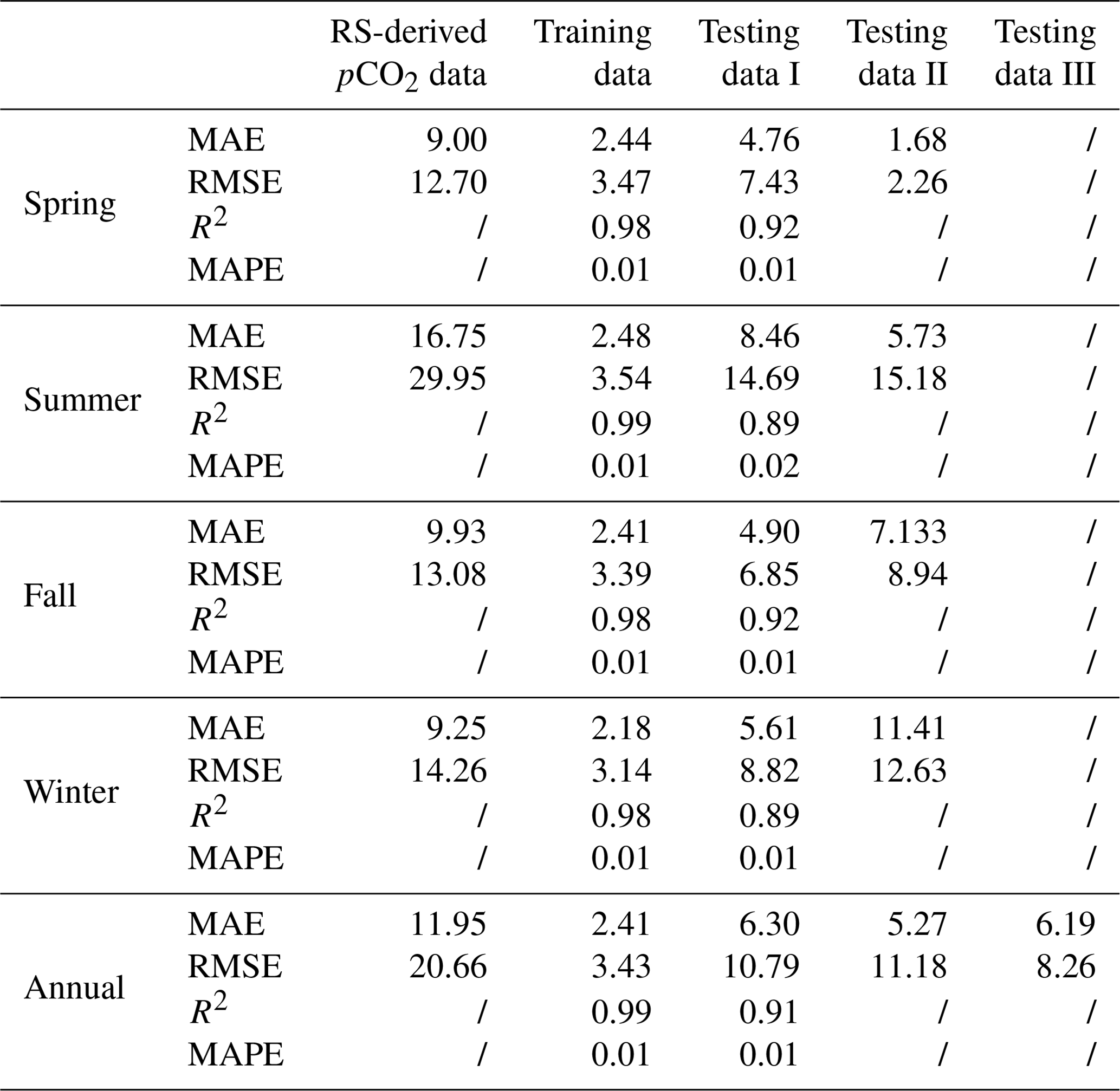
A grid-to-grid comparison was undertaken between the RS-derived pCO₂ and the in situ pCO₂ data (Table 2). The differences in between range from 35 to 120 µatm in the near-shore area. The largest biases occur in summer when the RMSE is up to 29.95 µatm (Table 2). Relatively large discrepancies may reflect the limitations of the current algorithm (MeSAA and nonlinear regression), which only considers biological processes and the turbidity induced by the Pearl River discharge (characterized by Chl a and the remote sensing reflectance at 555 nm (Rrs555) and does not take into account the riverine dissolved inorganic carbon and the input of other substances that may affect pCO₂ (Bai et al., 2015; Yu et al., 2022; Wang et al., 2021).

To remove the influence of the bias in RS-derived pCO₂ data on our reconstructed results, this study used the EOF method to compute the spatial patterns of the RS-derived pCO₂ data as input data instead of directly using the RS-derived pCO₂ data. Moreover, using EOF modes of the RS-derived pCO₂ as input data in the reconstructed model can provide spatial constraints on the pCO₂ reconstruction.

Table 2 Biases between the seasonal remote-sensing-derived pCO₂ data and in situ pCO₂ data and between the reconstructed and the in situ pCO₂ data (µatm). The remote-sensing-derived pCO₂ data during 2003–2019 are from http://www.SatCO2.com, and the source of the in situ data can be found in Table 1. The reconstructed pCO₂ data are from Sect. 3; all data were gridded into 0.05^∘ × 0.05^∘; the slash ($/$) means no data). MAE is the mean absolute error. RMSE is the root mean square error. R² is the coefficient of determination. MAPE is the mean absolute percentage error.

2.4 Other data

The RS-derived SST data produced by MODIS (Moderate Resolution Imaging Spectroradiometer; https://oceancolor.gsfc.nasa.gov/, last access: 8 October 2022) are adopted in our reconstruction. The uncertainty in this dataset in the SCS is ∼0.27^∘ (Qin et al., 2014). For sea surface salinity (SSS) data, Wang et al. (2022) found relatively large differences between different open-source SSS databases (i.e., multi-satellite fusion data from https://podaac.jpl.nasa.gov/, last access: 8 October 2022; model data from https://climatedataguide.ucar.edu/, last access: 8 October 2022; multidimensional covariance model data from https://resources.marine.copernicus.eu/, last access: 8 October 2022) and the in situ SSS data. Thus, Wang et al. (2022) produced an RS-derived SSS database using machine learning methods based on the MODIS Aqua remote sensing data. The bias between the RS-derived SSS (Wang et al., 2022) and in situ data was near zero (mean absolute error, MAE, of ∼0.25). Next, we used Chl a (from https://oceancolor.gsfc.nasa.gov/, last access: 8 October 2022) as an indicator of biological influence, which has a bias of ∼0.35 on a log scale and ∼115 % in the SCS (Zhang et al., 2006). Atmospheric pCO₂ also influences sea surface pCO₂ through air–sea CO₂ exchange. We chose the atmospheric CO₂ mole fraction (xCO₂) data from the monthly mean CO₂ concentrations measured at the Mauna Loa Observatory, Hawaii (https://gml.noaa.gov/, last access: 8 October 2022), and then calculated the atmospheric pCO₂ values from xCO₂ using the method in Li et al. (2020).

3 Methods

The pCO₂ reconstruction procedure is shown in Fig. 4. It includes (1) data processing and (2) model training and testing. For the former, we first gridded the in situ data and RS-derived pCO₂ data into 0.05^∘ × 0.05^∘ boxes with a monthly temporal resolution. Second, we filled missing pCO₂ measurements with the RS-derived pCO₂ data, according to Fay et al. (2021; see more details in Sect. 3.1). We then used EOF to ignore any biases in the RS-derived pCO₂ dataset itself or from the pCO₂ filling method. Third, the gridded in situ pCO₂ data and their corresponding RS-derived data were divided into a training set (90 %) and a testing set (10 %) to calculate the pCO₂ retrieval model. To ensure that the model had sufficient training samples in the coastal area, we divided the entire SCS into two regions along the 200 m isobath (as shown in Fig. 5). The data from these two regions were divided into training and testing sets with the same ratios listed above (9:1) and then combined to obtain the final training and testing sets. Note that all the data used in the machine learning have been interpolated on the same grid.

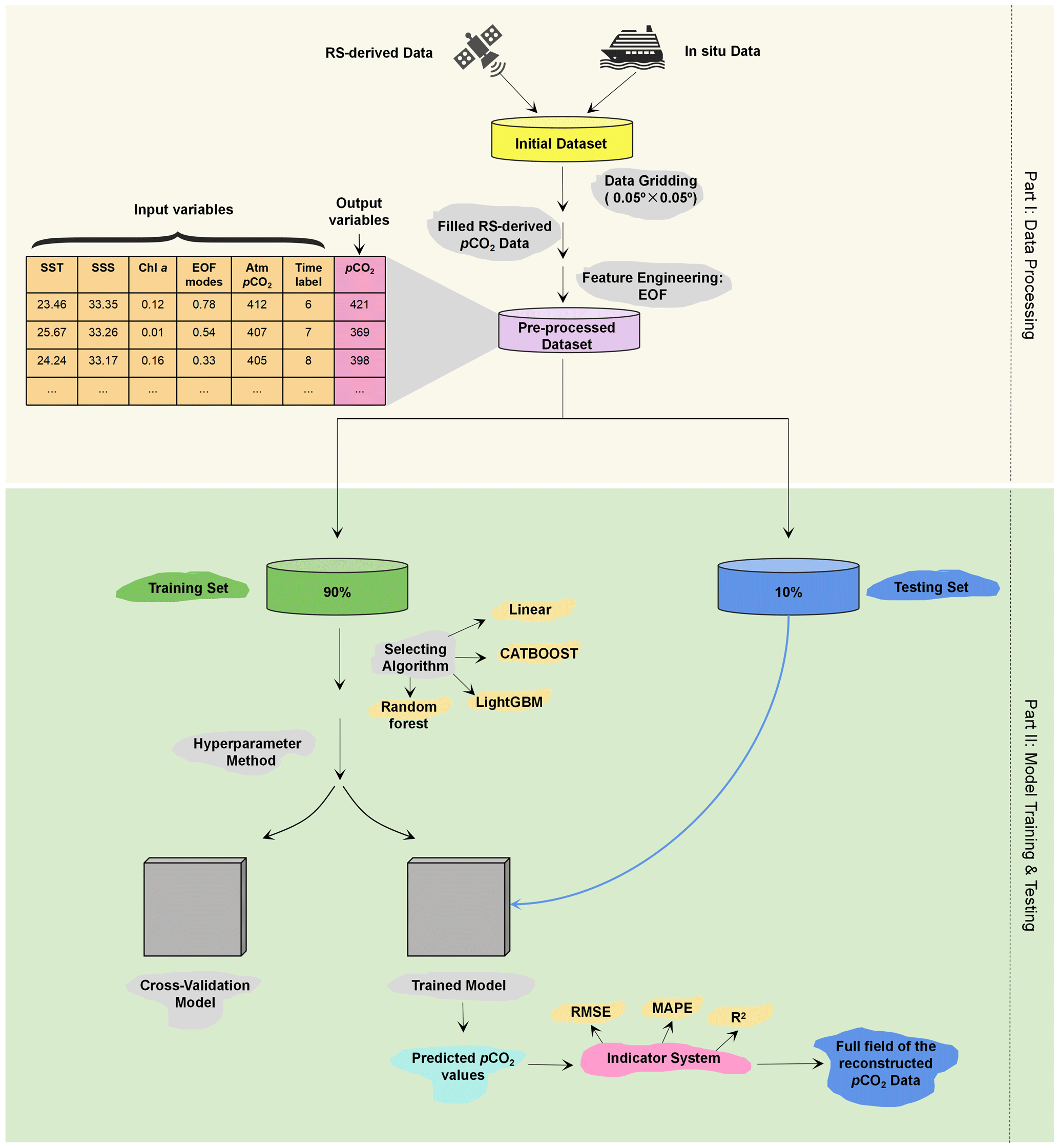
Figure 4 Procedure for the reconstruction of surface water pCO₂ using machine learning. RS-derived data are remote-sensing-derived data. RMSE is the root mean square error. MAPE is the mean absolute percentage error. R² is the coefficient of determination. MAE is the mean absolute error.

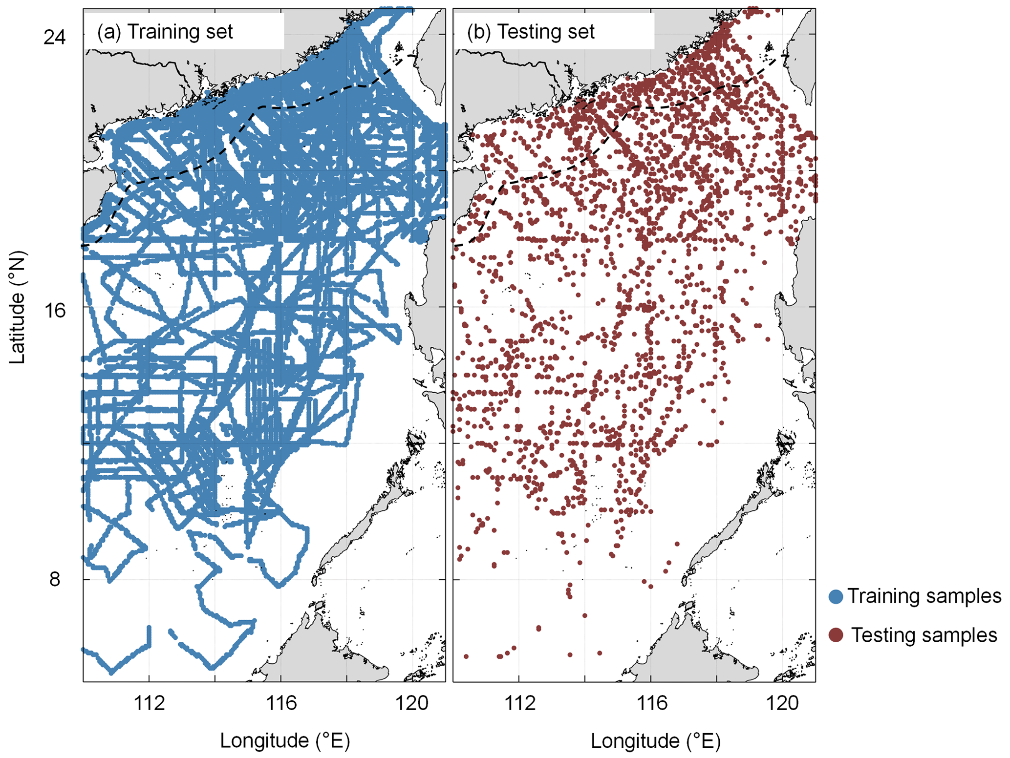
Figure 5 Spatial distributions of training samples (a) and testing samples (b). The dashed black line shows the 200 m isobath.

For model training and testing, we chose a relatively reliable algorithm to undertake the pCO₂ reconstruction. Next, we determined the optimal range of the parameters using hyperparameter methods (code from https://github.com/optuna/, last access: 8 October 2022) for the training set. The final optimal parameter values were then determined using the K-fold and cross-validation methods (code from https://github.com/suryanktiwari/Linear-Regression-and-K-fold-cross-validation, last access: 8 October 2022) for the training set. These optimal parameters were applied to the chosen algorithm. Finally, the testing set was used to verify the accuracy of the pCO₂ retrieval algorithm produced by the training set, and some indicators of the model's accuracy were calculated. More detailed methods employed in the present study are described below.

3.1 Remote sensing data filling

As mentioned in the SatCO₂ platform (http://www.SatCO2.com), RS-derived pCO₂ datasets have some missing values. Thus, we used the pCO₂ data-filling method, suggested by Fay et al. (2021), to obtain the missing data points. First, a scaling factor for a filled month was calculated according to Eq. (1):

$$\begin{array}{}\text{(1)}& {\text{sf}}_{p{\mathrm{CO}}_{\mathrm{2}}}={\text{mean}}_{x,y}\left({\displaystyle \frac{p{\text{CO}}_{\mathrm{2}}^{\mathrm{ens}}}{p{\text{CO}}_{\mathrm{2}}^{\mathrm{clim}}}}\right),\end{array}$$

where ${\text{sf}}_{p{\mathrm{CO}}_{\mathrm{2}}}$ is the scaling factor, $p{\text{CO}}_{\mathrm{2}}^{\mathrm{ens}}$ is the monthly RS-derived pCO₂ data, and $p{\mathrm{CO}}_{\mathrm{2}}^{\mathrm{clim}}$ is the monthly climatology RS-derived pCO₂ data. x and y indicate that we took the area-weighted average over longitude (x) and latitude (y) to produce the monthly sf${}_{p{\mathrm{CO}}_{\mathrm{2}}}$ value. Then, the filled portion of the data can be calculated from the $p{\text{CO}}_{\mathrm{2}}^{\mathrm{clim}}$ data multiplied by the sf_pCO2 value (see Fay et al., 2021, for details of this method).

Briefly, this filling method scales the climatological monthly pCO₂ field values to fill in the missing measurements. Therefore, although specific values may be biased, the interpolated measurements still retain the main spatial distribution pattern of the filled months.

3.2 Feature engineering and selection

As mentioned above, the pCO₂ data-filling method may bias some of the actual values. To avoid the influence of such biases on the reconstructed results, instead of directly using the RS-derived pCO₂ data as features in our reconstructed model, we used the EOF method to obtain the main spatiotemporal distribution patterns of the RS-derived pCO₂ data as features in our reconstructed model. The EOF reflects the spatial commonality of variables shown in the time series, and thus it is widely used to calculate spatial patterns of climate variability (e.g., Levitus et al., 2005; Dye et al., 2020; McMonigal and Larson, 2022). Typically, the spatial commonality of variables (EOF modes) is found by computing the eigenvalues and eigenvectors of a spatially weighted anomaly covariance matrix of a field. Each EOF mode's corresponding variance represents its degree of interpretation of the spatial pattern of a variable. For each of the 12 months, the cumulative variance contribution of the first eight EOF values was consistently >90 %, indicating that it could explain the main pCO₂ spatial characteristics during each month; we therefore selected them as features.

The features selected in our reconstructed model can be divided into two main categories. In the first category, the features are related to the underlying physicochemical mechanisms controlling the pCO₂ distribution; for example, SST exerts a primary control on the seasonal variations in surface water pCO₂ in the northern SCS (Zhai et al., 2005; Chen et al., 2007; Li et al., 2020). In the second category, they provide spatiotemporal information for the pCO₂ reconstruction. Previous studies (Landschützer et al., 2014; Laruelle et al., 2017; Denvil-Sommer et al., 2019) have shown that Chl a plays a critical role in fitting the influence of biological activity to pCO₂, especially in the northern SCS (Landschützer et al., 2014; Laruelle et al., 2017; Denvil-Sommer et al., 2019). Sutton et al. (2017) suggest that increasing atmospheric pCO₂ controls the overall increase in seawater pCO₂. For the features that provide spatiotemporal information for the pCO₂ reconstruction, in the present study we selected the first eight EOF values of pCO₂ as the main spatial distribution feature and the monthly information of the in situ datasets as the temporal feature.

3.3 Algorithm selection

Ensemble learning, which is the process of training multiple machine learning models and combining their output to improve the reliability and accuracy of predictions, is one of the most powerful machine learning techniques (e.g., Zhan et al., 2022; Cheng et al., 2020). In other words, several different models are used as the basis to develop an optimal predictive model. There are two main ways to employ ensemble learning, namely bagging (to decrease the model's variance) or boosting (to decrease the model's bias). The random forest algorithm (code from https://scikit-learn.org/stable/, last access: 6 May 2022) is an extension of the bagging method, as it utilizes both bagging and feature randomness to create an uncorrelated forest of decision trees. The light gradient-boosting machine (LightGBM; code from https://github.com/microsoft/LightGBM/, last access: 6 May 2022) is a gradient-boosting framework that uses tree-based learning algorithms. LightGBM can be used for regression, classification, and other machine learning tasks; it exhibits rapid, high-performance as a machine learning algorithm. CatBoost (code from https://github.com/catboost/, last access: 6 May 2022) is a gradient-boosting algorithm which improves prediction accuracy by adjusting weights according to the data distribution and by incorporating prior knowledge about the dataset. This can help to reduce overfitting and improve general performance.

From the above options, we chose three ensemble learning algorithms as the machine-learning-based regression portion and multilinear regression methods (Wang et al., 2021) as the linear regression portion. We then used the K-fold and cross-validation methods to verify the applicability of different regression algorithms in the pCO₂ reconstruction for seasonal training data. The results show that, in summer, the CatBoost algorithm yields the best degree of accuracy, with an RMSE of 16 µatm (Table 3). In contrast, the RMSE of LightGBM was 27 µatm and that of random forest (RF) was 26 µatm. The RMSE was nearly 20 µatm, using the linear regression algorithm employed by Wang et al. (2021). Thus, CatBoost appears to provide a reliable algorithm for reconstructing pCO₂. In the other three seasons, however, using different algorithms resulted in minor differences (∼2 µatm in RMSE).

Table 3 RMSEs associated with different algorithms in the four seasons.

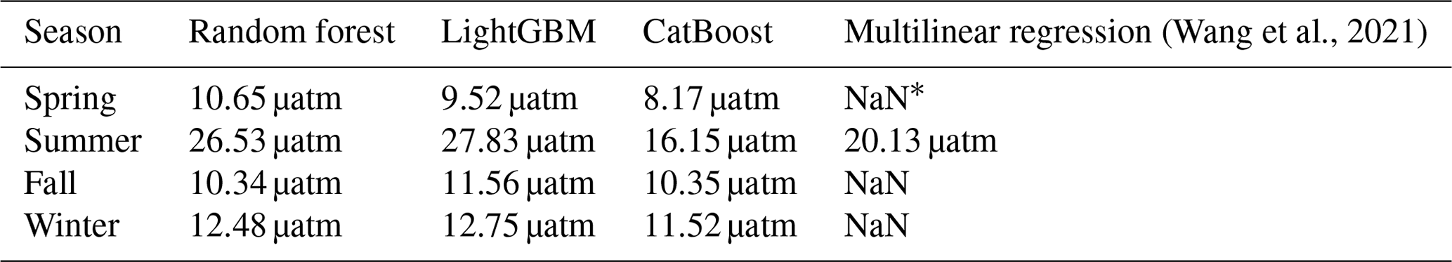
^* NaN stands for missing values.

3.4 Evaluation metrics

It is necessary to evaluate the accuracy of any model based on certain error metrics before applying it to specific scenarios. Common model evaluation metrics include RMSE, mean absolute percentage error (MAPE), R² (coefficient of determination), and MAE.

The mean squared error (MSE) is the standard deviation of the residuals (prediction error), and the residuals are the distances between the fitted line and the data points (i.e., the residuals show the degree of concentration of the reconstructed data around the regression line). In regression analysis, RMSE is commonly used to verify experimental results. To assess bias, the RMSE needs to combine the magnitude of the model data and is calculated as follows:

$$\begin{array}{}\text{(2)}& \mathrm{RMSE}=\sqrt{{\displaystyle \frac{\mathrm{1}}{n}}\sum _{i=\mathrm{1}}^n(y_i-y_{\mathrm{r}i}{)}^{\mathrm{2}}},\end{array}$$

where y stands for the in situ data, y_r represents the reconstructed data, and n is the number of data points.

The MAPE is a statistical measure used to define the accuracy of a machine learning algorithm on a particular dataset. It is commonly used because, compared to other metrics, it uses a percentage to measure the magnitude of the bias and is easy to understand and interpret; the lower the value of the MAPE, the better a model is at forecasting. MAPE is calculated as follows:

$$\begin{array}{}\text{(3)}& \mathrm{MAPE}={\displaystyle \frac{\mathrm{1}}{n}}\sum _{i=\mathrm{1}}^n{\displaystyle \frac{\mathrm{|}{y}_i-y_{\mathrm{r}i}\mathrm{|}}{\mathrm{|}{y}_i\mathrm{|}}}.\end{array}$$

The regression error metric, the coefficient of determination (R²), can describe the performance of a model by evaluating the accuracy and efficiency of the modeled results; i.e., it indicates the magnitude of the dependent variable, as calculated by the regression model, that can be explained by the independent variable. It is calculated as follows:

$$\begin{array}{}\text{(4)}& R^{\mathrm{2}}=\mathrm{1}-{\displaystyle \frac{\sum _{i=\mathrm{1}}^n(y_i-\stackrel{\mathrm{‾}}{y_i}{)}^{\mathrm{2}}}{\sum _{i=\mathrm{1}}^n(y_i-y_{\mathrm{r}i}{)}^{\mathrm{2}}}}.\end{array}$$

MAE is the average absolute difference between the in situ data (true values) and the model output (predicted values). The sign of these differences is ignored so that cancelations between positive and negative values do not occur. It is calculated as follows:

$$\begin{array}{}\text{(5)}& \mathrm{MAE}={\displaystyle \frac{\mathrm{1}}{n}}{\sum }_i^n\mathrm{|}{y}_i-y_{\mathrm{r}i}\mathrm{|}.\end{array}$$

3.5 Uncertainty

In previous studies, RMSE and MAE have primarily been used to represent the uncertainties in reconstructed datasets. However, this expression of uncertainty ignores the sensitivity of the reconstructed model to the features; i.e., the biases that the features themselves pass to the reconstructed model are ignored. Moreover, it is clearly unreasonable to use a single RMSE or MAE value to represent the entire region because the spatial bias pattern in the coastal region clearly differs from that in the basin.

Thus, here we present a novel method for calculating uncertainty, as shown below:

$$\begin{array}{}\text{(6)}& \begin{array}{rl}& \text{Uncertainty}\\ & =\text{MAX}\left(\right[{\displaystyle \frac{\sum _{i=\mathrm{1},j=\mathrm{1},k=\mathrm{1}}^n\frac{\mathrm{|}\text{OR\_Monthly\_Data}(i,j,k)-\text{Obs\_Monthly\_Data}(i,j,k)\mathrm{|}}{\text{Obs\_Monthly\_Data}(i,j,k)}}{\text{num}\left(i\right)+\text{num}\left(j\right)}},\mathrm{\dots },\\ & \cdot {\displaystyle \frac{\sum _{i=\mathrm{1},j=\mathrm{1},k=n}^n\frac{\mathrm{|}\text{OR\_Monthly\_Data}(i,j,k)-\text{Obs\_Monthly\_Data}(i,j,k)\mathrm{|}}{\text{Obs\_Monthly\_Data}(i,j,k)}}{\text{num}\left(i\right)+\text{num}\left(j\right)}}\left]\right)\\ & \cdot \mathrm{100}\mathit{\%}\cdot p{\mathrm{CO}}_{\mathrm{2}}\mathit{\_}\text{recon}+\left({\displaystyle \frac{\partial p{\mathrm{CO}}_{\mathrm{2}}}{\partial \text{Feature}}}\right)\mathrm{d}\text{Feature}\end{array}.\end{array}$$

Equation (6) includes two terms. The first term is the conservative bias between the reconstructed pCO₂ fields and the in situ data, and the second is the sum over sensitivity of the reconstructed model to the features. For the first term in Eq. (6), k stands for the kth month, OR_Monthly_Data(ijk) stands for the kth monthly reconstructed data at longitude (i) and latitude (j), and Obs_Monthly_Data(ijk) stands for the kth monthly in situ data at longitude (i) and latitude (j). Therefore, MAX in the first term stands for the maximum of the k monthly bias ratios. And pCO₂_recon stands for the reconstructed pCO₂ data. In the second term, dFeature stands for the bias of the features. We conducted a sensitivity analysis using a chain rule to evaluate the influence of these biases in the features on pCO₂. Then we estimated pCO₂ changes due to the variabilities in these features by constraining these features based on our model and computed $\frac{\partial p{\mathrm{CO}}_{\mathrm{2}}}{\partial \text{Feature}}$. For example, for $\frac{\partial p{\mathrm{CO}}_{\mathrm{2}}}{\partial \text{SST}}$, we only changed the value of SST and kept the values of the other features constant to calculate the effect of each additional unit of SST on the simulated pCO₂.

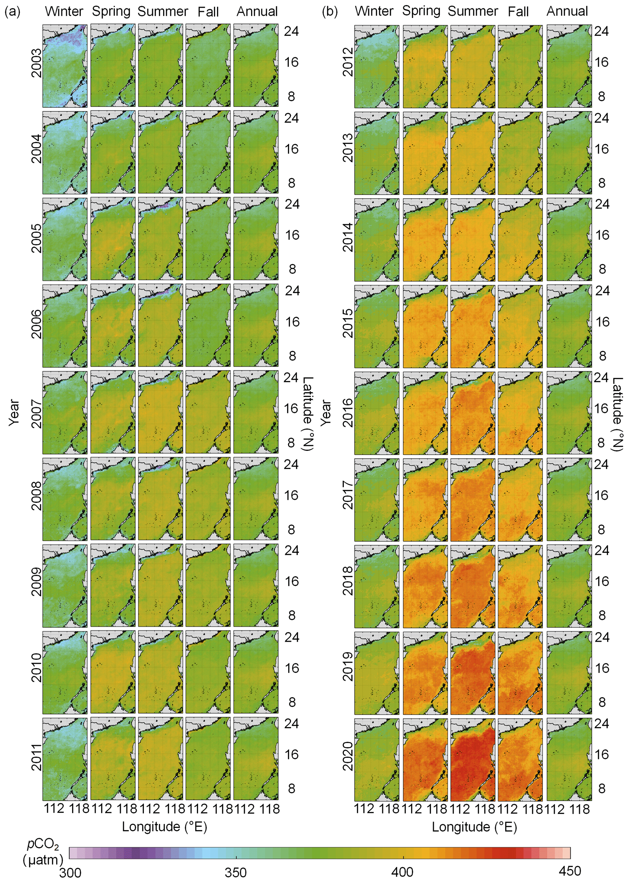
Figure 6 Reconstructed seasonal and annual pCO₂ fields in the South China Sea from 2003 to 2020 (a, 2003–2011; b, 2012–2020).

4 Results and discussion

4.1 Results

The reconstructed pCO₂ fields show relatively low values in the northern coastal region of the study area and generally high values in the middle and southern basins (Fig. 6). The continuous changes in the spatiotemporal distribution can be found in the reconstruction results (Fig. 6). The reconstructed pCO₂ fields show a trend of slow but sustained increases from 2003 to 2020. Spatial patterns of pCO₂ change between 2003 and 2020, such that the coastal portion of the northern SCS shows relatively complex variability from multiple controlling factors, such as coastal upwelling, river plumes, biological activity, etc. However, pCO₂ values in the middle and southern basins are relatively homogeneous, as they are mainly controlled by atmospheric pCO₂ forcing and SST. Temporal changes in pCO₂ between 2003 and 2020 are relatively large (∼44 µatm) in summer and relatively small (∼33 µatm) in winter.

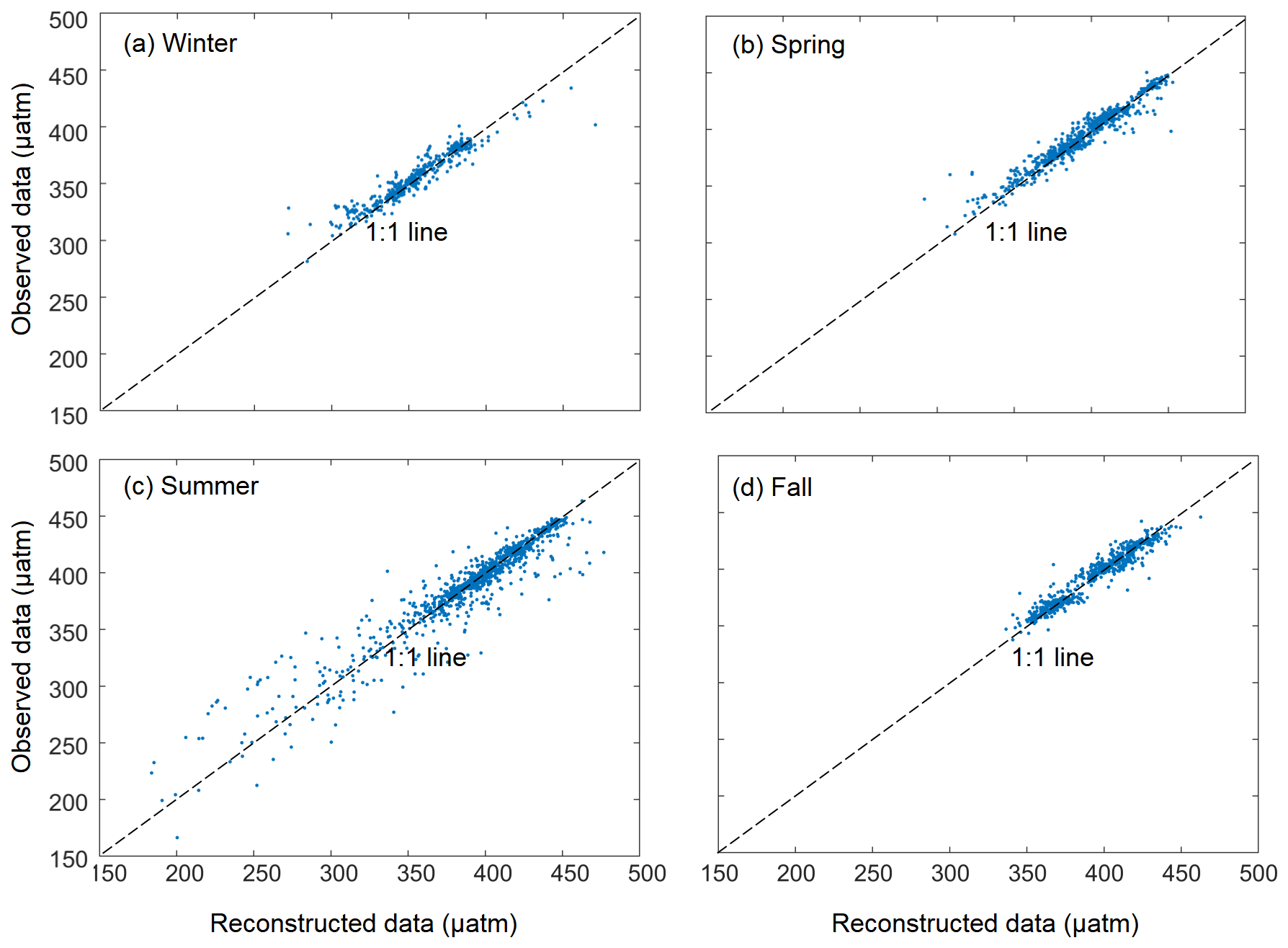
Figure 7 Comparisons between the monthly reconstructed and in situ pCO₂ values for the testing set. The monthly results are grouped into the four seasons, including (a) winter, in December, January, and February, (b) spring, in March, April, and May, (c) summer, in June, July, and August, and (d) fall, in September, October, and November.

4.2 Model validation

Figure 7 compares the monthly reconstructed and in situ data. For the training dataset, the reconstructed pCO₂ fields of the four seasons fit the in situ data well (Fig. 7), with an average RMSE of 3.43 µatm and an average MAE of 2.14 µatm (Table 2). For the testing sets, although there are some outliers, most of the reconstructed pCO₂ data are consistent with the in situ data, with RMSE averaging 10.79 µatm and MAE averaging 6.30 µatm. The R² of the testing set is ca. 0.91. In terms of MAPE, the accuracies of the four seasonal models are all around 99 % (Table 2), with the highest value for spring data and the lowest value for summer data. The relatively large bias (14.67 µatm) in the summer may be the influence of relatively complex regional processes, such as river plumes and upwelling. The four evaluation metrics indicate that our reconstructed pCO₂ field is highly accurate in simulating both the training and testing sets.

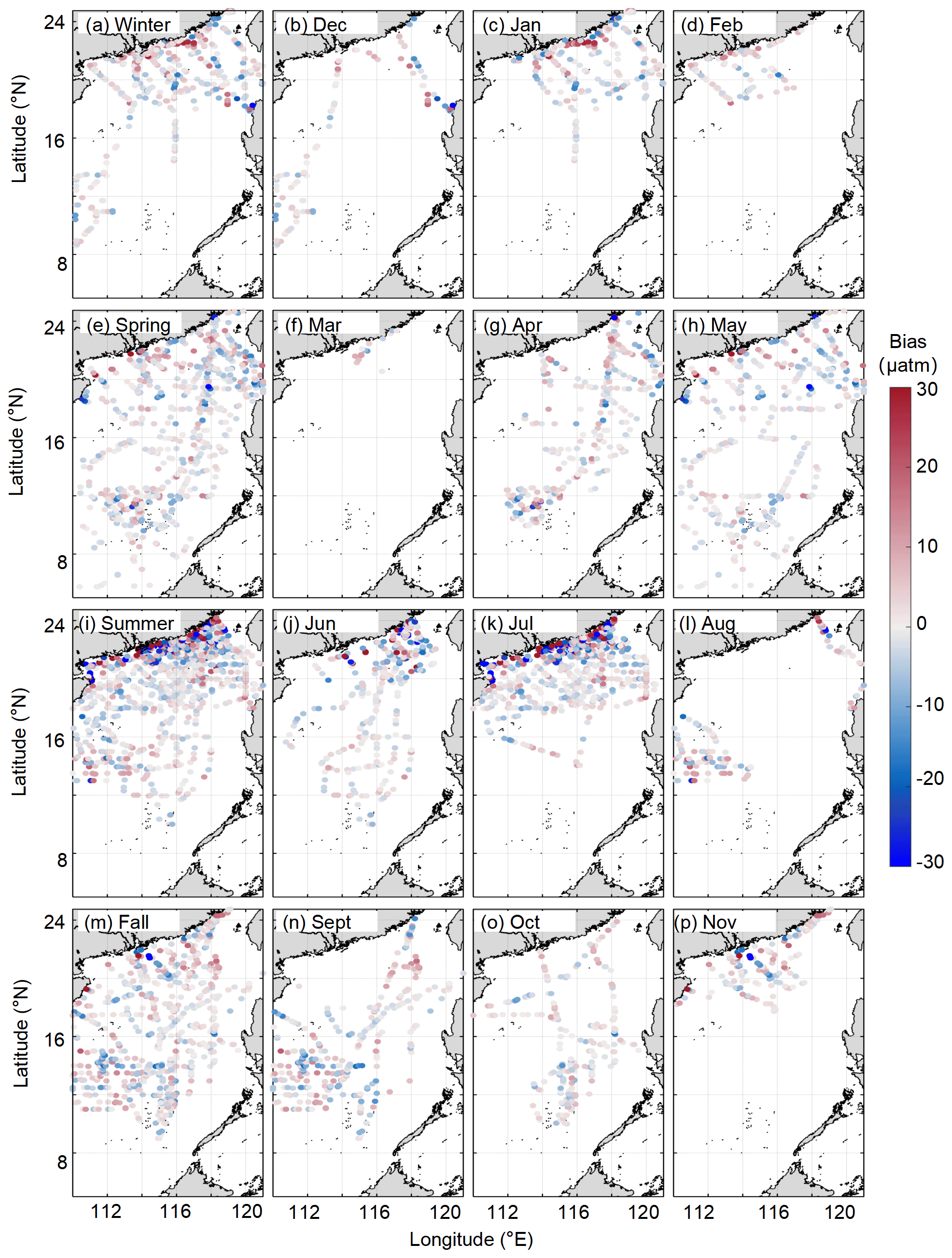
Figure 8 Differences between the reconstructed and in situ pCO₂ data, both seasonally and monthly, for the testing set, including (a) winter, (b) December, (c) January, (d) February, (e) spring, (f) March, (g) April, (h) May, (i) summer, (j) June, (k) July, (l) August, (m) fall, (n) September, (o) October, and (p) November).

The distributions of the biases between the reconstructed fields and the in situ data for both the training and testing datasets can be found in Fig. 8. In terms of the temporal pattern, the larger biases were more concentrated in the summer. For the spatial pattern, the biases in the northern coastal area are much greater than those in the basin. However, 95 % of the biases are $<\pm \mathrm{10}$ µatm; therefore, our reconstructed dataset exhibits relatively high accuracy.

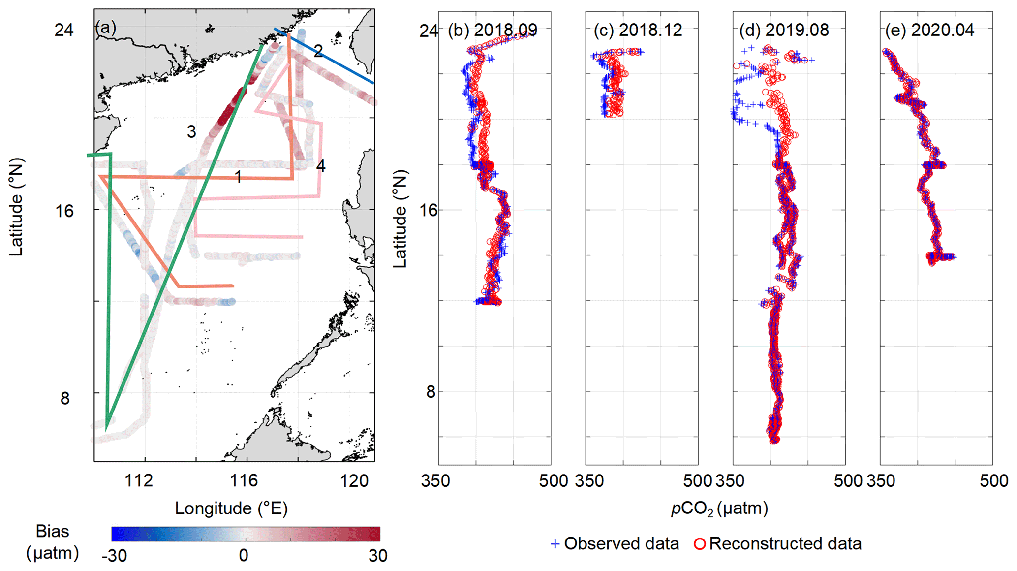
Figure 9 Difference between the reconstructed pCO₂ data and four independently tested in situ datasets during the four seasons. In panel (a), the numbers 1–4 represent September 2018 (b), December 2018 (c), August 2019 (d), and April 2020 (e), respectively.

Figure 9 shows the bias between our reconstructed fields and the four independent in situ datasets corresponding to the four seasons. This validation can verify the accuracy of the retrieval algorithm for months without observations, namely the applicability of the retrieval algorithm extrapolation. This comparison shows that the retrieval algorithm is relatively accurate in the basin, with a near-zero bias (MAE of ∼8 µatm; Fig. 9a). The largest bias occurs in the Pearl River plume area in summer (∼35 µatm). The retrieval algorithm also has a high accuracy for pCO₂ spatial variability, except in the Pearl River plume area in summer (22–20^∘ N; Fig. 9b–e). The effect of the Pearl River plume on the pCO₂ spatial distribution in our retrieval algorithm is smaller than that shown by the in situ data. This is because, at around the survey time (24–28 August 2019), a large amount of precipitation (∼30 mm d⁻¹; https://psl.noaa.gov/data/gridded/data.ncep.reanalysis2.surface.html, last access: 8 October 2022) occurred around the Pearl River estuary region (24–20^∘ N), which led to the intensification of the Pearl River plume. The plume has relatively low pCO₂ values that eventually decreased the observed values along the coast. However, the monthly average runoff of the Pearl River during that month (August 2019; http://www.pearlwater.gov.cn/, last access: 8 October 2022; see the Pearl River plume index in Wang et al., 2022) was low, indicating that our retrieval algorithm is still highly reliable from the perspective of monthly averages. Thus, the inconsistencies between the reconstructed (monthly average) and the in situ datasets are mainly due to the differences in the timescales of the remote sensing and the in situ data. The reconstructed data in this study were determined on a monthly scale, while the temporal resolution of the in situ data were on the order of hours. It is clear that relatively pronounced short-term changes in pCO₂, such as the diurnal variability caused by short-term heavy precipitation, cannot be reflected in the reconstructed data.

Dai et al. (2022) produced a time series of in situ data from 2003 to 2019 at the SEATs station, which we used here to validate the accuracy of the long-term trends of our model data (results shown in Fig. 10). The long-term trend of reconstructed pCO₂ data at the SEATs station is largely consistent with the in situ data, with differences mainly found before 2005. Thus, the long-term trend produced in our reconstructed model is also highly reliable.

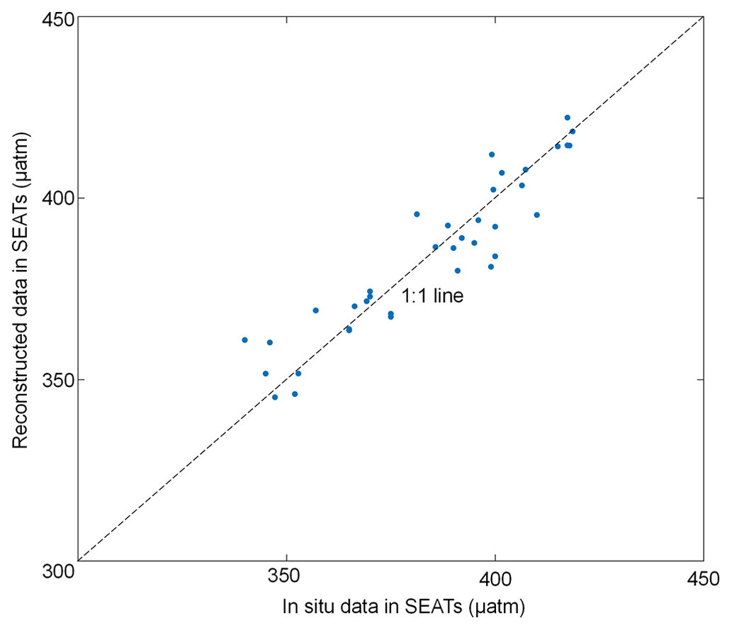
Figure 10 Comparison of the reconstructed pCO₂ with in situ data at the Southeast Asia Time-series Study (SEATs) station (116^∘ E, 18^∘ N). The in situ data are from Dai et al. (2022), which were calculated from dissolved inorganic carbon and total alkalinity values.

4.3 Uncertainties

As shown in Table 2, our reconstructed data have a high degree of accuracy, with an RMSE of ∼10 µatm and MAE of ∼6 µatm. According to Eq. (6), the bias of RS-derived pCO₂ data used in the second term of Eq. (6) is ∼21 µatm (Table 2), the bias of SST is ∼0.27 ^∘C (Qin et al., 2014), the bias of SSS is ∼0.33 (Wang et al., 2022), and the bias of Chl a is ∼115 % (Zhang et al., 2006). We then estimated the pCO₂ changes due to the variations in these features by constraining these features based on our model and computed $\frac{\partial p{\mathrm{CO}}_{\mathrm{2}}}{\partial \text{Feature}}$.

The overall uncertainty in the reconstructed dataset is greater in the coastal area (∼13 µatm) than in the basin (∼10 µatm; Fig. 11a), and this spatial pattern is mainly determined by the second term in Eq. (6). The spatial distribution of the first term in Eq. (6) (Fig. 11b), calculated from a max bias ratio, is consistent with that of pCO₂ (Fig. 11b). The second term in Eq. (6) (Fig. 11c) is calculated from the propagation of the bias from each variable (Fig. 11c). The Chl a bias (Fig. 11f) shows that it has the greatest effect on the reconstruction, among all the features (Fig. 11f). Although the bias of the RS-derived pCO₂ data is relatively large, the final influence that it has on the results from the retrieval algorithm is negligible due to the use of the EOF method (Fig. 11g).

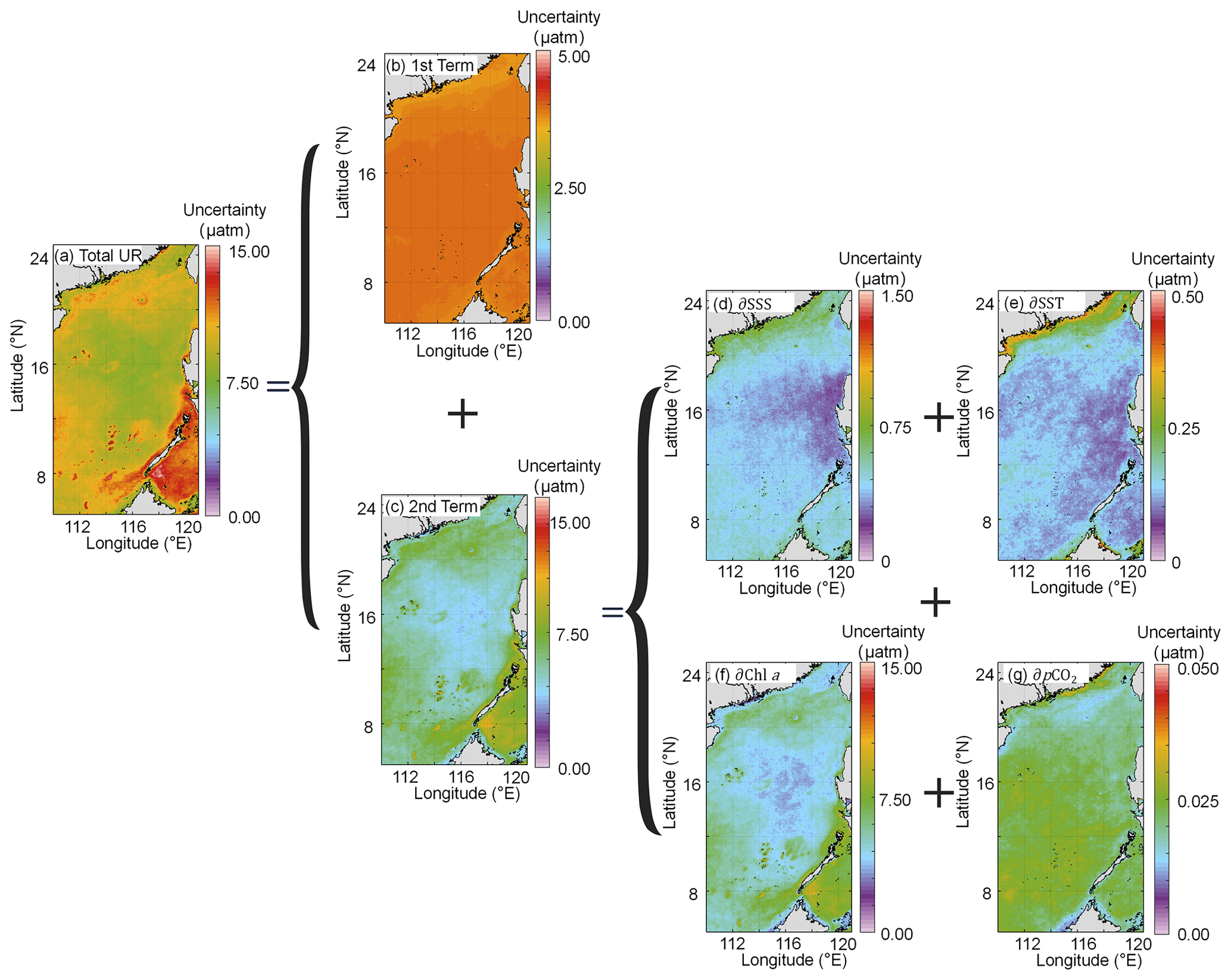
Figure 11 Uncertainties in the reconstructed pCO₂ fields. (a) Total uncertainty in Eq. (6). (b) The first term of Eq. (6). (c) The second term of Eq. (6). (d) ($\frac{\partial p{\mathrm{CO}}_{\mathrm{2}}}{\partial \text{SSS}})\text{dSSS}$ in the second term of Eq. (6). (e) ($\frac{\partial p{\mathrm{CO}}_{\mathrm{2}}}{\partial \text{SST}})\text{dSST}$ in the second term of Eq. (6). (f) ($\frac{\partial p{\mathrm{CO}}_{\mathrm{2}}}{\partial \text{Chl}a})\text{dChl}a$ in the second term of Eq. (6). (g) ($\frac{\partial p{\mathrm{CO}}_{\mathrm{2}}}{\partial \text{RS\_derived\_}p{\text{CO}}_{\mathrm{2}}})\text{dRS\_derived\_}p{\text{CO}}_{\mathrm{2}}$ in the second term of Eq. (6).

4.4 Spatial and temporal pCO₂ features

The climatological monthly reconstructed pCO₂ fields are shown in Fig. 12. The highest values occur in May and June, and the lowest values occur in January. In winter, pCO₂ first decreases in December and then increases after January; the pCO₂ value is ca. 325 µatm in the northern coastal area and ca. 350 µatm in the basin. In spring, pCO₂ gradually increases from the basin to the northern coastal area, and the high pCO₂ values in the central basin gradually expand outward starting in April. In summer, pCO₂ gradually declines, starting in June. In fall, pCO₂ increases from north to south, and the southern region shows consistently high values.

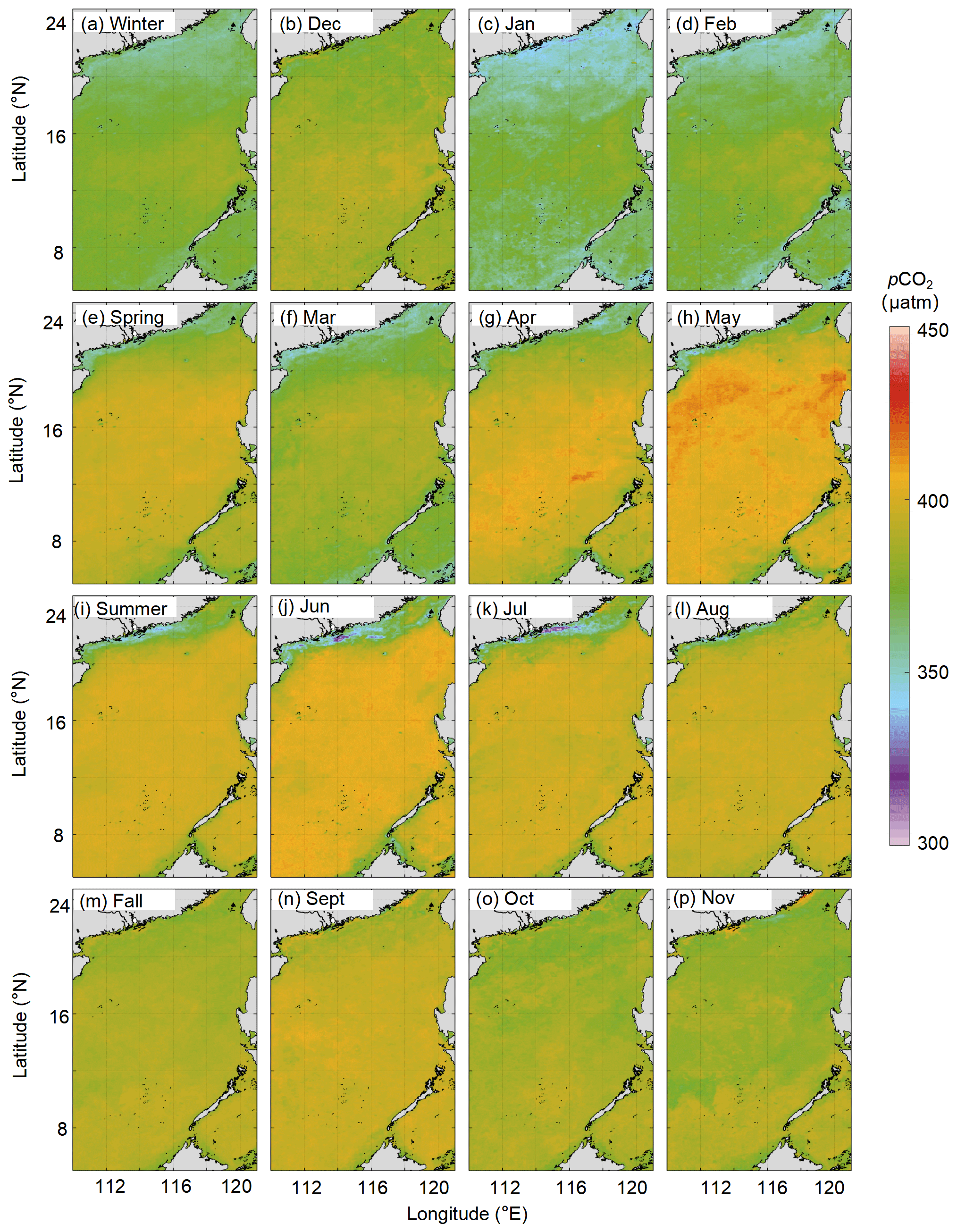
Figure 12 Long-term (2003–2020) seasonal and monthly averaged pCO₂ field (µatm). (a) Winter. (b) December. (c) January. (d) February. (e) Spring. (f) March. (g) April. (h) May. (i) Summer. (j) June. (k) July. (l) August. (m) Fall. (n) September. (o) October. (p) November.

To better show specific regions in the northern coastal area, we magnified the reconstructed pCO₂ fields at locations north of 18^∘ N (Fig. 13). The reconstructed pCO₂ fields successfully reflect the influence of the meso–microscale processes on pCO₂ in this northern coastal area of the SCS. For example, in winter, the relatively low pCO₂ values, which last into early spring, are mainly controlled by the low SST and the high pCO₂ around Luzon Strait affected by winter upwelling. In summer, the reconstructed pCO₂ field shows that the influence of the Pearl River plume on pCO₂ is the strongest in July and lasts until September; it also effectively shows the influence of coastal upwelling in the northeastern shelf (∼23^∘ N, 117^∘ E). Thus, our reconstructed pCO₂ fields clearly reflect the spatial pattern of the in situ pCO₂ (Fig. 3), which are generally consistent with previously reported patterns (Li et al., 2020; Zhai et al., 2013; Gan et al., 2010).

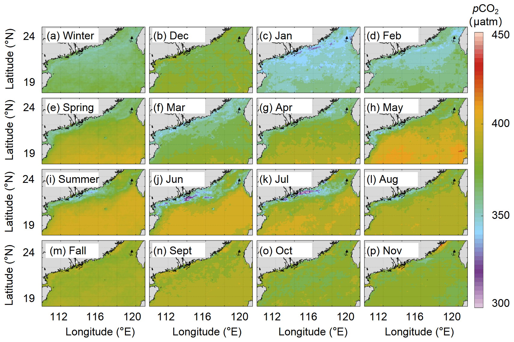
Figure 13 Long-term (2003–2020) seasonal and monthly averaged pCO₂ field in the region north of 18^∘ N (µatm). (a) Winter. (b) December. (c) January. (d) February. (e) Spring. (f) March. (g) April. (h) May. (i) Summer. (j) June. (k) July. (l) August. (m) Fall. (n) September. (o) October. (p) November.

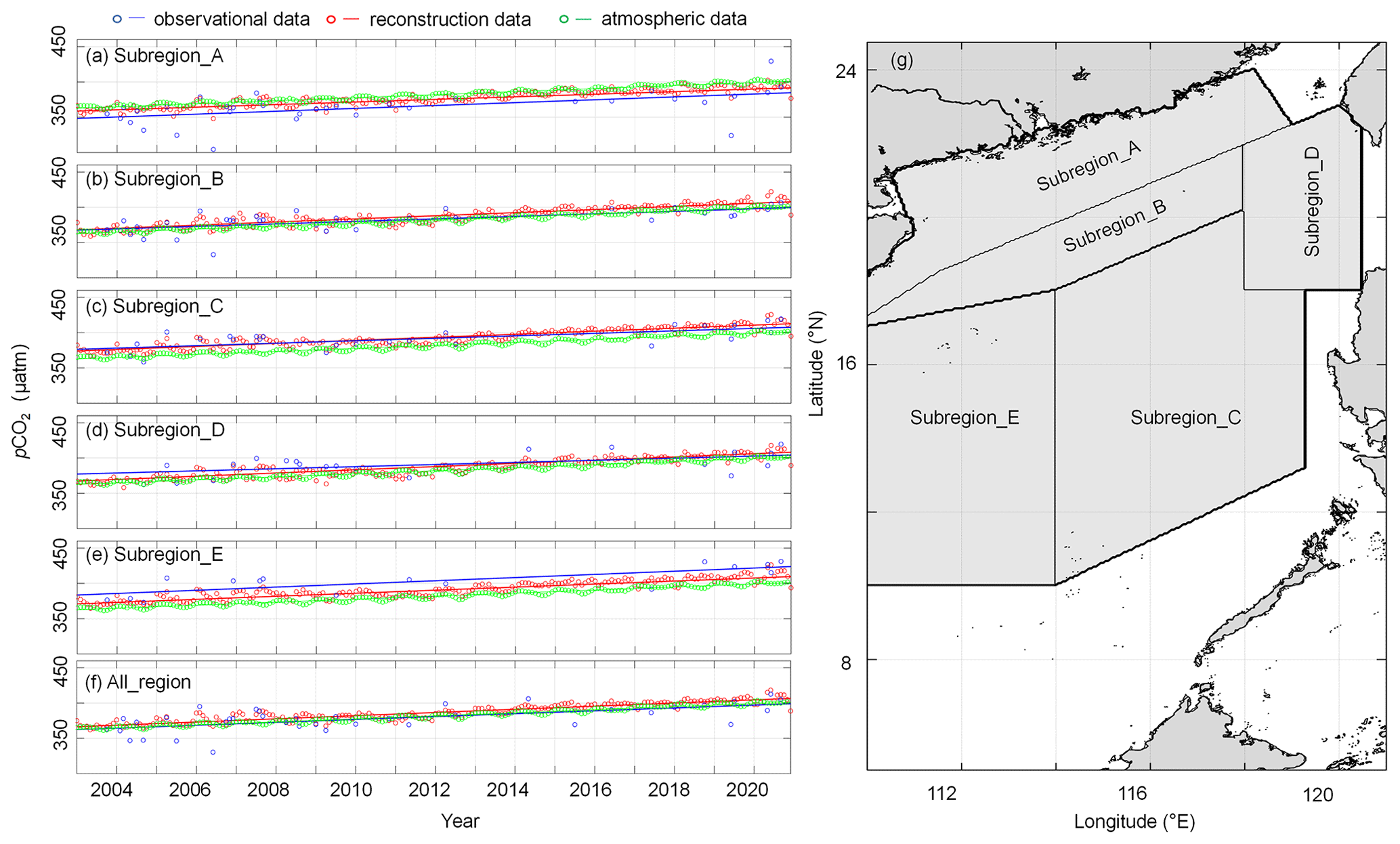
Figure 14 Time series of spatially averaged monthly pCO₂ data in five subregions (a–e) and the entire South China Sea (f) under study. The subregions are shown in panel (g). The lines indicate the deseasonalized long-term trend of the spatially averaged monthly pCO₂ data for each subregion, with the slopes shown in Table 3. The deseasonalized method can be found in Landschützer et al. (2016).

Table 4 Deseasonalized long-term trend of the spatially averaged monthly pCO₂ data for each subregion of the South China Sea (µatm yr⁻¹).

We divided SCS into five subregions, according to Li et al. (2020). In Fig.14, Subregion_A stands for the northern coastal area of the SCS, Subregion_B stands for the slope area of the northern SCS, Subregion_C stands for the SCS basin, Subregion_D stands for the region west of the Luzon Strait, and Subregion_E stands for the slope and basin area of the western SCS. All_region indicates the whole region containing the five subregions described above. We then calculated the deseasonalized long-term trend of spatially averaged monthly data for each subregion, and the results are shown in Fig. 14 and Table 3. This deseasonalized trend is consistent with that of the in situ data, and its uncertainty is on the 95 % confidence interval (much lower than that shown by the in situ data). We can thus also infer that the long-term trend of our reconstructed data shows high reliability in all subregions and that our data can serve as an important basis for predicting future changes in pCO₂ in the SCS.

In Fig. 14a–e, we found that the sea surface pCO₂ of the entire SCS is slightly higher than the atmospheric pCO₂, indicating that the SCS is a weak source of atmospheric CO₂. This conclusion is consistent with previous studies (e.g., Li et al., 2020). Moreover, compared to the rate of atmospheric CO₂ increase (∼2.2 µatm yr⁻¹), for Subregion_A, the pCO₂ trend is much slower than that of atmospheric pCO2, and the spatially averaged monthly mean pCO₂ is lower than the atmospheric pCO2. Thus, carbon accumulation in this region is expected to increase in the future. For Subregion_C and Subregion_E, the spatially averaged monthly mean pCO₂ is higher than the atmospheric pCO₂; thus, these two regions will still provide a weak source of atmospheric CO₂ in the future. Finally, whether Subregion_B and Subregion_D act as a source or sink of the atmospheric CO₂ is influenced by seasonal changes and physical processes. Subregion_B can be a zone of significant sink of atmospheric CO₂, as demonstrated by its low sea surface pCO₂ when the Pearl River plume spreads more widely in summer. In contrast, in winter, when the Kuroshio intrusion is strong, both Subregion_B and Subregion_D have high sea surface pCO₂, indicating both subregions are sources of atmospheric CO₂.

5 Data availability

The data (the reconstructed pCO₂ data, the in situ pCO₂ data before 2018 (0.5^∘ × 0.5^∘), and the remote-sensing-derived CO₂ data) for this paper are available at https://doi.org/10.57760/sciencedb.02050 (Wang and Dai, 2022).

6 Conclusions

Based on the machine learning method, we reconstructed the sea surface pCO₂ fields in the SCS with an 0.05^∘ × 0.05^∘ spatial resolution over the last 2 decades (2003–2020) by calculating the statistical relationship between the in situ pCO₂ data and RS-derived data. The input data we used in machine learning include RS-derived data (sea surface salinity, sea surface temperature, and chlorophyll), the spatial patterns of pCO₂ calculated by EOF, atmospheric CO₂, and time labels (month). The machine learning method (CatBoost) used in this study was facilitated by the EOF method, which provides spatial constraints for the data reconstruction. In addition to the typical machine learning performance metrics, we present a novel method for uncertainty calculation that incorporates the bias of both the reconstruction and the sensitivity of reconstructed models to its features. This method effectively shows the spatiotemporal patterns of bias and makes up for the spatial representation of the typical performance metrics.

We validate our reconstruction with three independent testing datasets, and the results show that the bias between our reconstruction and in situ pCO₂ data in the SCS is relatively small (about 10 µatm). Our reconstruction successfully captures the main features of the spatial and temporal patterns of pCO₂ in the SCS, indicating that we can use these reconstructed data to further analyze the effect of meso–microscale processes (e.g., the Pearl River plume and CCC) on sea surface pCO₂ in the SCS.

We divided the SCS into five subregions, separately calculated the deseasonalized long-term trend of pCO₂ in each subregion, and compared them with the long-term trend of atmospheric pCO₂. Our results show that the reconstructed data are consistent with those of in situ data. Moreover, the strength of the CO₂ sink in the northern SCS shows an increasing trend, whereas pCO₂ trends in other subregions are essentially the same as that of atmospheric pCO₂.

This high spatiotemporal resolution of sea surface pCO₂ data is helpful to clarify the controlling factors of pCO₂ change in the SCS and may be useful to predict changes in CO₂ source or sink patterns in this system.