Nunataryuk field campaigns: understanding the origin and fate of terrestrial organic matter in the coastal waters of the Mackenzie Delta region

Climate warming and related drivers of soil thermal change in the Arctic are expected to modify the distribution and dynamics of carbon contained in perennially frozen grounds. Thawing of permafrost in the Mackenzie River watershed of northwestern Canada, coupled with increases in river discharge and coastal erosion, triggers the release of terrestrial organic matter (OMt) from the largest Arctic drainage basin in North America into the Arctic Ocean. While this process is ongoing and its rate is accelerating, the fate of the newly mobilized organic matter as it transits from the watershed through the delta and into the marine system remains poorly understood. In the framework of the European Horizon 2020 Nunataryuk programme, and as part of the Work Package 4 (WP4) Coastal Waters theme, four field expeditions were conducted in the Mackenzie Delta region and southern Beaufort Sea from April to September 2019. The temporal sampling design allowed the survey of ambient conditions in the coastal waters under full ice cover prior to the spring freshet, during ice breakup in summer, and anterior to the freeze-up period in fall. To capture the fluvial–marine transition zone, and with distinct challenges related to shallow waters and changing seasonal and meteorological conditions, the field sampling was conducted in close partnership with members of the communities of Aklavik, Inuvik and Tuktoyaktuk, using several platforms, namely helicopters, snowmobiles, and small boats. Water column profiles of physical and optical variables were measured in situ, while surface water, groundwater, and sediment samples were collected and preserved for the determination of the composition and sources of OMt, including particulate and dissolved organic carbon (POC and DOC), and colored dissolved organic matter (CDOM), as well as a suite of physical, chemical, and biological variables. Here we present an overview of the standardized datasets, including hydrographic profiles, remote sensing reflectance, temperature and salinity, particle absorption, nutrients, dissolved organic carbon, particulate organic carbon, particulate organic nitrogen, CDOM absorption, fluorescent dissolved organic matter intensity, suspended particulate matter, total particulate carbon, total particulate nitrogen, stable water isotopes, radon in water, bacterial abundance, and a string of phytoplankton pigments including total chlorophyll. Datasets and related metadata can be found in Juhls et al. (2021) (https://doi.org/10.1594/PANGAEA.937587).

1 Introduction

Major components of the Arctic cryosphere are currently exposed to acute changes due to accelerated climate warming rates at high latitude (IPCC, 2018, 2019; AMAP, 2021). In the Northern Hemisphere, nearly a quarter of the landmass is influenced by permafrost, which is perennially cryotic ground (Brown et al., 1997; Gruber, 2012; Obu et al., 2019). Permafrost soils store approximately 60 % of the world's soil carbon (C) in 15 % of the global soil area (Schuur et al., 2015; McGuire et al., 2018; Hugelius et al., 2014). When frozen, the C contained in this reservoir is stable. But rising air temperatures and associated alterations in soil thermodynamics, in addition to modifications in snow regimes (Romanovsky et al., 2010), are now leading to the release of C-rich terrestrial organic matter (OMt) in potentially climate-relevant amounts (Guo et al., 2007; Schuur et al., 2015; Schaefer et al., 2014). While permafrost thaw is ongoing and its rate is accelerating (Camill, 2005; Biskaborn et al., 2019), the fate of the newly mobilized OMt as it transits from watersheds to rivers and into coastal waters of the Arctic Ocean remains poorly understood.

Increasing amounts of organic C originating from permafrost thaw delivered to arctic coastal waters via river discharge (Mcguire et al., 2009; Tank et al., 2016) and rapidly eroding coastlines (Tanski et al., 2019; Wegner et al., 2015) may have significant impacts on both the cycling of C in the Arctic Ocean and the global C budget through complex physical (e.g., weathering, burial, and photodegradation) and biogeochemical (e.g., microbial degradation) processes (Guo et al., 2007; Vonk et al., 2014; Stedmon et al., 2011; Tanski et al., 2017). Gaining greater insight into these processes is crucial, as they may lead, among other things, to enhanced emissions of CO₂ or other greenhouse gases (Semiletov et al., 2013; Vonk et al., 2012; Vonk and Gustafsson, 2013; Tanski et al., 2019). Changes in primary production (Kipp et al., 2018) that sustain the marine arctic food web may also arise with unknown impacts on the communities that rely on these food sources (Fritz et al., 2017). While past studies have broadened our understanding of the riverine transport of nutrients, organic matter, and suspended sediments into coastal waters of the Arctic Ocean (McClelland et al., 2006; Stedmon et al., 2011; Holmes et al., 2012), assessments of the seasonal and interannual variations in OMt fluxes at the Pan-Arctic scale are still limited.

During the Canada Arctic Shelf Exchange Study (CASES, 2002–2004) expeditions and the Arctic River Delta Experiment (ARDEX, 2004), field sampling and satellite observations were conducted in coastal sites near the Mackenzie River mouth and along the shelf edge into the Beaufort Sea (CASES), as well as in the river's east and middle channels and throughout the delta (ARDEX), to explore both the biogeochemistry and photoreactivity of colored dissolved organic matter (CDOM) transported by rivers to Arctic shelf environments (Osburn et al., 2009). Later, in 2009, the MALINA oceanographic campaign took place in the Mackenzie River estuary and the Beaufort Sea systems during summer to document the stocks and the processes controlling carbon fluxes across meridional gradients between the estuary and the open ocean (Massicotte et al., 2021). While the MALINA expedition furthered our insights into the cycling of carbon across shelf–basin systems, it left knowledge gaps regarding the spatial dynamics of organic matter (OM) in the delta area of the Mackenzie, where the network of rivers empties its water and sediment into the Arctic Ocean. Furthermore, lacking from the otherwise extensive MALINA, CASES, and ARDEX datasets were measurements of the seasonal variations in OM sources, types, and fluxes, particularly during the spring freshet when river discharge rates peak.

While conducting fieldwork in key areas of the Mackenzie Delta region is challenging due to limited accessibility, estimating the fluxes of organic carbon (OC), including particulate (POC) and dissolved (DOC) forms, to arctic coastal waters via satellite observations is also challenging due to the complexity of the optical properties of marginal environments, frequent cloud cover, and low Sun elevation (IOCCG, 2015). Nevertheless, knowledge of arctic shelf and coastal water optical properties has recently been expanded (Matsuoka et al., 2011, 2014; Juhls et al., 2019), providing the foundation for algorithms estimating DOC and POC concentrations using satellite ocean color data (Doxaran et al., 2012; Matsuoka et al., 2013, 2017). Moving forward, the expansion of ground-truthing data to train remote sensing algorithms is paramount to gain synoptic views in study regions with challenging accessibility. Such is the case for the meandering and complex network of rivers, transitional fluvial-to-marine zone, and coastal waters that characterize the Mackenzie Delta region, the largest Arctic drainage basin in North America. Limited accessibility to the coastal waters adjacent to the delta watershed has resulted in poor spatial coverage of this highly dynamic zone. As such, our understanding of organic matter transformation and processing along the land–ocean aquatic continuum, and specifically in the delta where fresh and saline waters meet, has been hampered (Fritz et al., 2017).

Scientists working in the framework of the European Horizon 2020 Nunataryuk programme, along with partners from the Inuvialuit Nunangit Sannaiqtuaq communities of Aklavik, Inuvik, and Tuktoyaktuk (Inuvialuit Settlement Region, ISR, Northwest Territories, Canada), conducted four expeditions in the coastal waters of the Beaufort Sea adjacent to the Mackenzie Delta region from April to September 2019. The seasonal field campaign aimed to determine the amount and quality of OM supplied to the Arctic Ocean via riverine and diffuse inputs (e.g., including submarine groundwater discharges that were investigated in July–August 2019) of the Mackenzie Delta region. Ultimately, the in situ characterization of OM (i.e., its origin, age, reactivity, lability, and optical properties) will feed the development of optical remote sensing algorithms and numerical modeling endeavors. In this article, we present an overview of the broad dataset acquired during the four field surveys conducted as part of the fourth Nunataryuk Work Package – WP4 Coastal Waters – in the Mackenzie Delta region. To our knowledge, the data collected in this difficult-to-access area and included in this paper are unprecedented, both in their spatial coverage of the fluvial-to-marine transition zone and their seasonal extent.

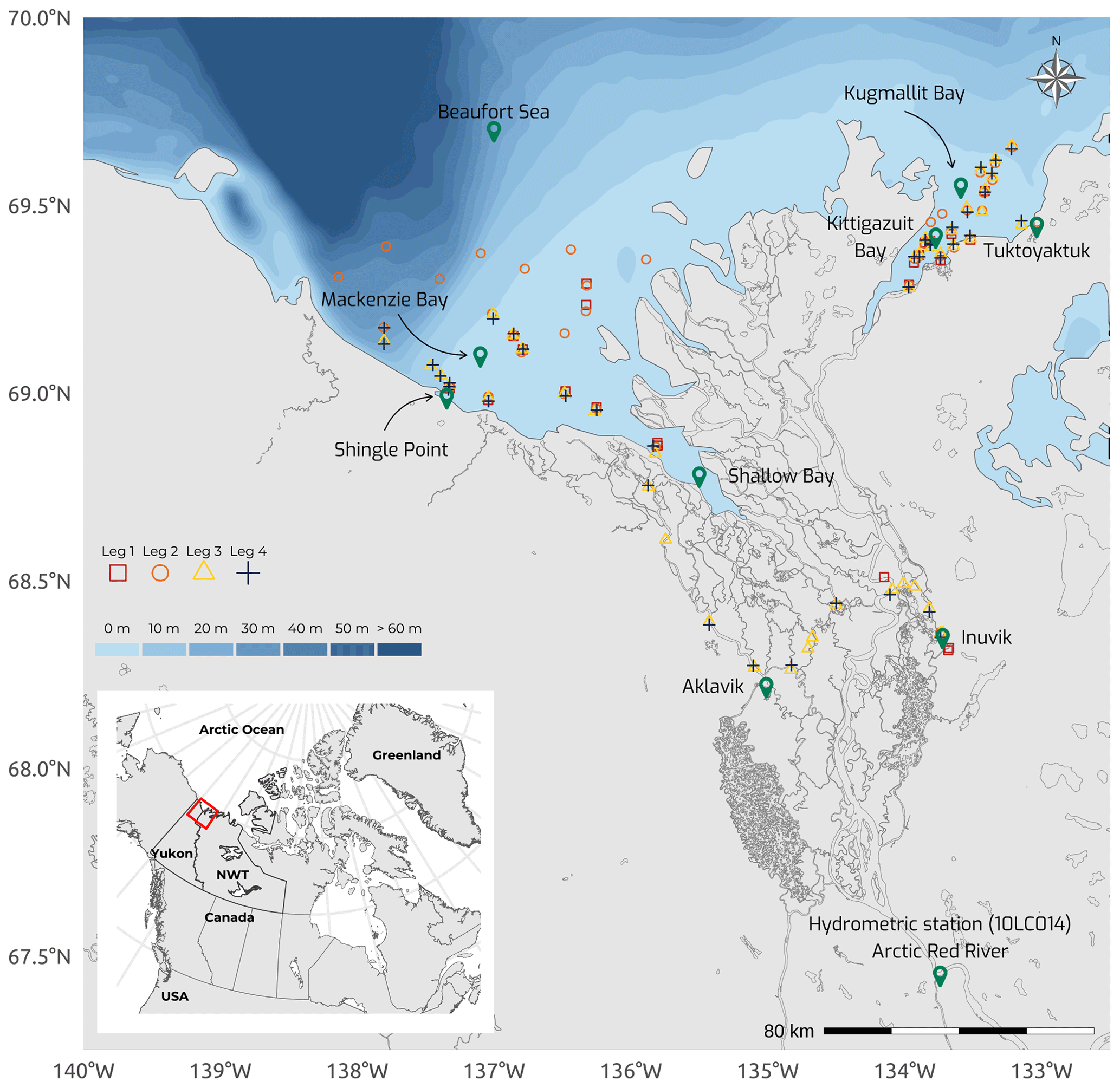
Figure 1 Map of the Mackenzie Delta region (Inuvialuit Settlement Region, Northwest Territories, Canada), with bathymetric features (from 0 to >60 m) of the coastal waters of the southern Beaufort Sea, showing the sampling stations during the four 2019 WP4 Nunataryuk field expeditions (Legs 1, 2, 3, and 4). Note that the Arctic Red River hydrometric station (10LC014) used to retrieve discharge rates (Fig. 3a) is shown. Leg 1 took place from 17 April to 3 May 2019, Leg 2 extended from 14 June to 4 July 2019, Leg 3 took place from 25 July to 8 August 2019, and Leg 4 was conducted from 26 August to 9 September 2019.

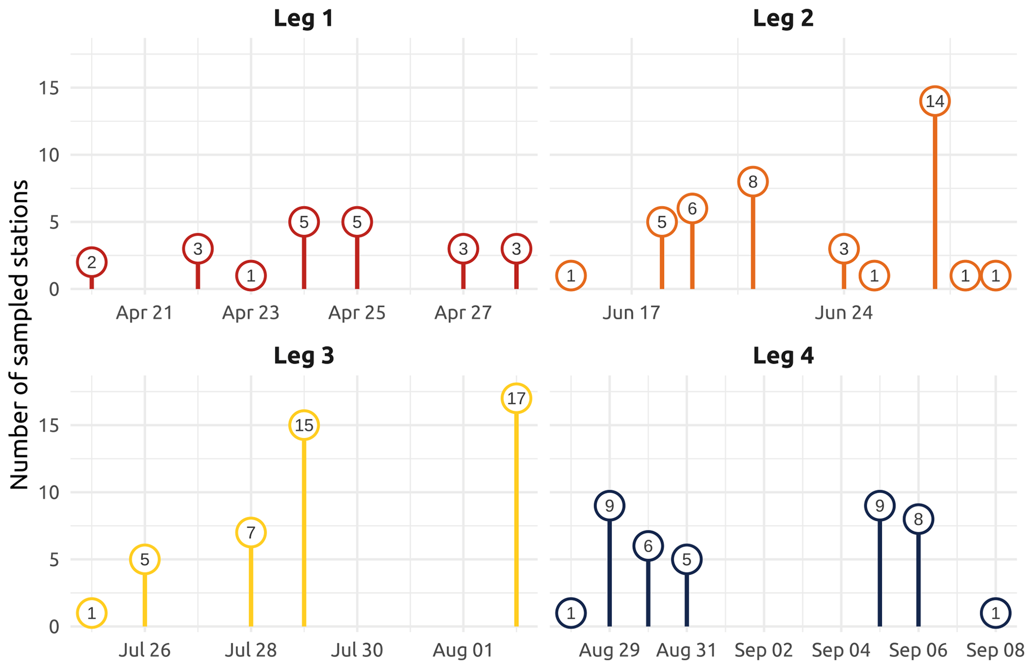
Figure 2 Number of sampled stations for each sampling day of the four main WP4 Nunataryuk expeditions (Legs 1, 2, 3, and 4) in 2019. Note that the groundwater field survey was conducted during Leg 3 in the vicinity of Tuktoyaktuk (Kugmallit Bay), where 29 water samples were collected at the nearshore (see Sect. 4.4.2).

2 Study area, environmental conditions, and sampling strategy

The field campaign was conducted in the coastal waters of the Beaufort Sea adjacent to the Mackenzie Delta region (ISR, Northwest Territories, Canada), within major embayments of the area, including Shallow Bay and Mackenzie Bay (in the west) and Kittigazuit Bay and Kugmallit Bay (in the east; see Fig. 1) in 2019 (see Fig. 2 for an overview of the sampling). When logistically possible, opportunistic sampling was also conducted in the channels of the Mackenzie River (68.26–69.65^∘ N, 138.14–133.03^∘ W; Fig. 1). The sampling was conducted following consultations at the Inuvialuit Game Council (8–9 March 2018) and a tour (16–23 February 2019) with local members, organizations, committees, municipal entities, and councils of three communities, namely Aklavik, Inuvik, and Tuktoyaktuk. The sampling periods were consensually selected with respect to traditional hunting–fishing grounds and activities of the northern community members of the ISR and in order to capture salient features of the Mackenzie River discharge dynamics (pre-freshet, freshet, and post-freshet; see Fig. 3a), salinity (Figs. 5 and C1), and considering a range of sea ice conditions in the coastal area (Fig. 4). Four field sampling periods were targeted. (1) Leg 1 took place from 17 April to 3 May 2019 (22 stations; see Fig. 2; see Sect. 4.4.1 for details on sediment sampling). (2) Leg 2 extended from 14 June to 4 July 2019 (40 stations; Fig. 2). (3) Leg 3 took place from 25 July to 8 August 2019 (45 stations; Fig. 2; see Sect. 4.4.2 for details on the parallel groundwater field survey). (4) Leg 4 was conducted from 26 August to 9 September 2019 (39 stations; Fig. 2; see Sect. 4.4.1 for details on sediment sampling).

Figure 3 (a) Mackenzie River discharge (m³ s⁻¹) from January 2019 to January 2020 shown as the gray line with overlain colored segments corresponding to Legs 1, 2, 3, and 4 (data from ArcticGRO; Arctic Red River ID 10LC014; 67.45^∘ N, 133.74^∘ W; Shiklomanov et al., 2021; https://arcticgreatrivers.org/discharge/, last access: 3 February 2023). The gray shaded area in panel (a) represents mean values (± standard deviation) of the climatology from 2000–2022. (b) Air temperature (^∘ C) from January 2019 to January 2020. The average (solid gray line) spread of air temperature data (gray points) and the 0 ^∘C threshold (dotted gray line) are presented. Colored segments correspond to Legs 1, 2, 3, and 4 sampling periods (data from Government of Canada, Environment and Climate Change Canada – Meteorological Service of Canada; measured at Tuktoyaktuk ID 2203914; 69.43^∘ N, 133.02^∘ W).

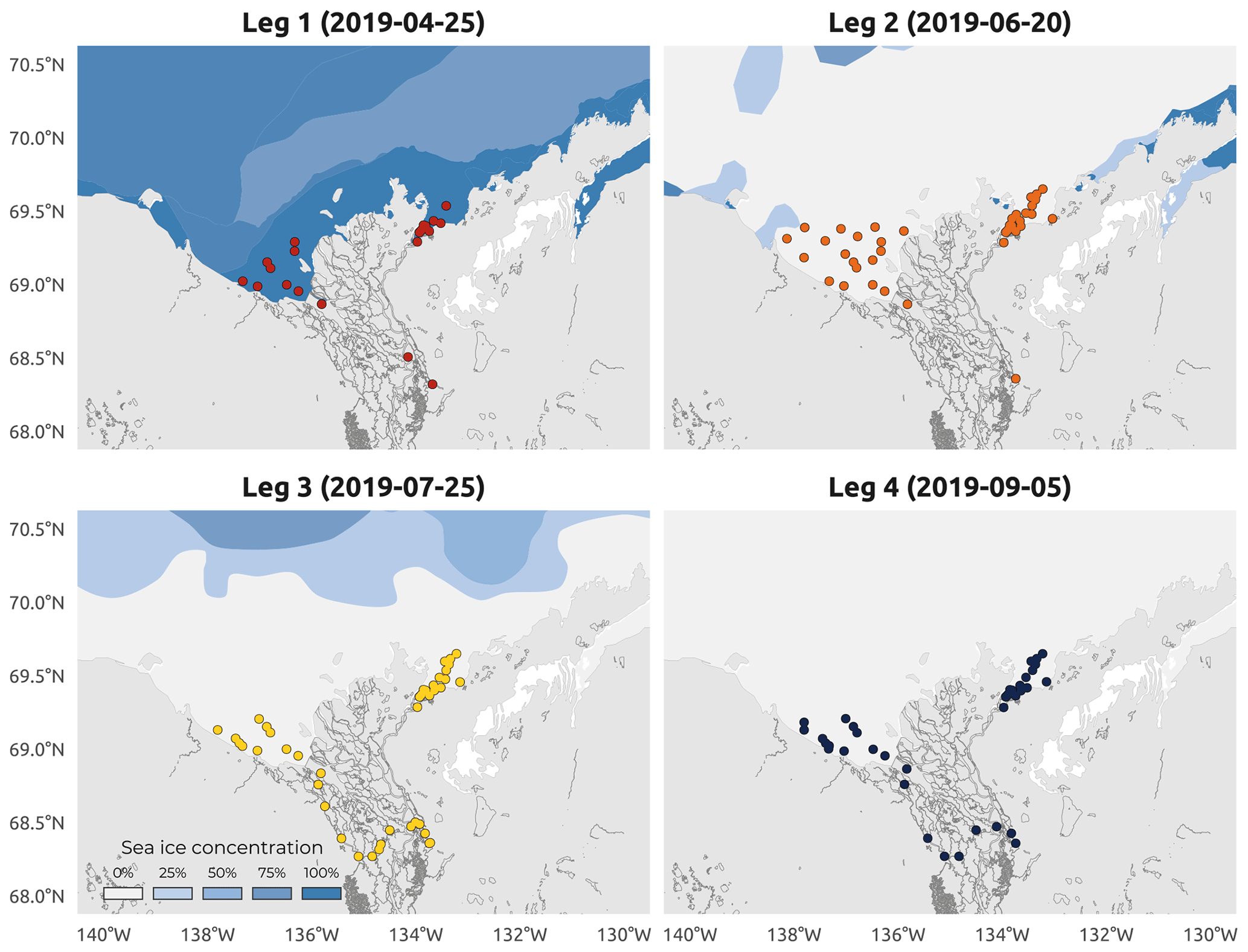
Figure 4 Sea ice concentration (SIC) in the coastal waters of the Beaufort Sea. Colored dots on each panel represent sampled stations during a specific Leg (1–4). Dates represent the middle of the sampling period of each Leg (1–4) of the WP4 Nunataryuk 2019 field campaign. Data are sourced from the National Snow and Ice Data Center (https://nsidc.org/data/G10033, last access: 26 September 2022). Note that there was unconsolidated ice during Leg 2.

The sampling conducted during Leg 1 encompassed pre-freshet conditions, as shown in Fig. 3a, with low river discharge, winter freezing air temperatures (Fig. 3b), and 75 % to 100 % sea ice concentration in the region sampled (Fig. 4a). The second expedition (Leg 2) closely followed the breakup of a thick barrier of rubble ice (stamukhi) that is generated each year by ice convergence at the outer edge of the land–fast sea ice in the coastal area near the Mackenzie River outflow (Reimnitz et al., 1978). Additionally, Leg 2 captured the peak of the annual Mackenzie River discharge (16 513 m³ s⁻¹; Fig. 3a) and warming air temperatures (>5 and <10 ^∘C; see Fig. 3b), with on average less than 25 % sea ice concentration over the sampling region (Fig. 4b). Sea ice cover had completely receded over the study site by Leg 3 (Fig. 4c), average air temperatures were at their highest (>10 and <15 ^∘C; Fig. 3b), and river discharge was still relatively high (11 226 m³ s⁻¹; Fig. 3a). Leg 3 captured the greatest extent in the salinity gradient covered by the sampling grid (Figs. 5 and 6a). Environmental conditions during Leg 4 were similar to those encountered during Leg 3, with the absence of sea ice (Fig. 4) and relatively high river discharge rates (Fig. 3a), albeit slightly cooler air (>5 and <10 ^∘C; Fig. 3b). Overall, discharge rates were similar to climatological means (2000–2022) for Leg 1 and Leg 4 but lower compared to the climatology during Leg 2 and Leg 3 (see Fig. 3a).

Given the wide range of environmental conditions encountered between the months of April and September, flexibility in sampling strategy was adopted, and various vehicles (Fig. A1) were used to ensure safe and efficient fieldwork. With the presence of consolidated sea ice in the coastal waters of the Beaufort Sea during Leg 1 (Fig. 4), helicopter flights were carried out from Inuvik to the western sector of the coastal waters (Shallow and Mackenzie bays) due to the large distance separating the sampling area and the nearest community (Aklavik), in addition to the impossibility to set up camp near the coast. Snowmobile trips were made out of Tuktoyaktuk to reach the targeted stations in the eastern sector (Kittigazuit and Kugmallit bays; see Fig. 1). To access the water column underneath the sea ice cover, a hole was drilled through the ice using a battery-powered auger. After each day of sampling, the water and sediment collected were light-protected and brought to the Western Arctic Research Center (WARC) of the Aurora Research Institute in Inuvik – either by air or ground (Inuvik–Tuktoyaktuk highway) – where the existing laboratories were used to immediately process, analyze, and/or package samples for later shipment. During Leg 2, the presence of unconsolidated sea ice (Fig. 4) imposed helicopter sampling in stationary flight above the stations (no landing) with the use of specialized hoisting gear for sampling in the western sector. To sample the eastern sector during Leg 2, small local boats (mostly fishing boats) were hired and launched from Tuktoyaktuk. Finally, during Legs 3 and 4, small local boats were chartered to reach the sampling sites. In the western sector, the field team made camp on Shingle Point (Fig. 1), while in the eastern sector, sampling was conducted from Tuktoyaktuk. Collected material was protected from the light and variations in temperature and sent by air or ground each day to the WARC laboratories in Inuvik for immediate processing. For the groundwater (GW) field survey conducted in parallel during Leg 3, sampling sites were reached using small boats and helicopter flights in the vicinity of Tuktoyaktuk (details in Sect. 4.4.2). Samples were collected and transported to a mobile laboratory built in the Tuktoyaktuk Community Learning Centre for immediate processing.

Table 1 Descriptions of the minimal variables included in each dataset.

3 Data quality control and data processing

The coherence and integrity of the data were first visually assessed to remove errors stemming from measurement procedures, methods, and instruments. Cleaned data were grouped and structured into ASCII files, each constructed to gather variables of the same type (e.g., nutrients). In each of these files, a minimum number of variables (columns) was always included to help the merging of different datasets (Table 1). More than 150 different variables were measured during the WP4 Nunataryuk 2019 field expeditions. The complete list of variables is presented in Table 2 (Sect. 4.4), along with statistical summaries such as average, standard deviation, and ranges. The final processed, quality-controlled datasets and related metadata are available in Juhls et al. (including 13 associated datasets 2021). In the following sections, a subset of these variables, along with the methods used to collect and measure them, are presented. The data visualization shown in this article was performed with R 4.2.0 (R Core Team, 2022). The code used to process the figures and tables is publicly available (https://github.com/PMassicotte/nunataryuk_data_paper, last access: 3 February 2023) under the MIT license. The purpose of this paper is to provide an overview of the availability of data for use in future studies and not to offer an in-depth analysis of the measurements conducted.

Figure 5 Spatial distribution of the CTD-measured surface salinity (conductivity) during the four WP4 Nunataryuk expeditions (Legs 1, 2, 3, and 4) in 2019. Note the log10 color scale used to visualize the salinity gradient. Surface here refers to samples collected between 0.30 and 1.66 m.

Figure 6 Box plots showing an overview of the (a) salinity, (b) water temperature, (c) δ¹⁸O, and a set of organic-matter-related parameters measured during the four Legs. (d) a_CDOM(443) (absorption of colored dissolved organic matter measured at 443 nm). (e) DOC (dissolved organic matter) and f SUVA₃₅₀ (specific ultraviolet absorbance at 350 nm, i.e., a_CDOM(350) $/$ DOC) (g) SPM (suspended particulate matter). (h) POC (particulate organic carbon). (i) a_p(443) (absorption of particulate matter measured at 443 nm). Boxes represent the interquartile range (IQR), the horizontal lines show the medians, while the vertical lines show data spread with min/max whiskers. Note that while vertical profiles were conducted, only surface samples (from 0.3 to 1.66 m) were used in these box plots.

4 Data description: an overview

4.1 Physical and optical data

Vertical profiles of underwater conductivity (e.g., Appendix C; Fig. C1) and conservative temperature and depth (CTD) were measured at each site by deploying and immediately recovering two RBR sensors. These were a RBRmaestro³ model (depth rating of 100 m) during Leg 1 and a RBRconcerto³ model (depth rating of 50 m) during Legs 2, 3, and 4. Both Figs. 5 and 6 only show the surface data collected between 0.30 and 1.66 m for underwater conductivity (Figs. 5 and 6a) and conservative temperature (Fig. 6b). The sensors, chosen for their high vertical resolution and accuracy (see below), were deployed either alone (Leg 1) or fitted to a frame together with various optical sensors (Legs 2, 3, and 4). As recommended by the instrument manufacturer, the conductivity cell was placed more than 15 cm away from any other structure. Both sensors were factory-calibrated prior to the expeditions and deployed either through the ice (Leg 1) or directly into the water column (Legs 2, 3, and 4) from helicopters or boats. The manufacturer gives an initial accuracy of ±0.003 mS cm⁻¹ for the conductivity, ±0.002 ^∘C for the temperature, and ±0.05 % for the sensors' maximum depth (i.e., 0.05 m for the RBRmaestro³ model and 0.025 m for the RBRconcerto³ model that have been used; see https://info.rbr-global.com/hubfs/RBR Standard Instruments RIG 0008815revB.pdf, last access: 5 April 2023). As the stations were relatively shallow, from a few meters to a maximum of 28 m, the descent rate was kept slow at between 0.05 and 0.20 m s⁻¹. Examples of vertical temperature–salinity profiles are presented in Fig. C1 (Appendix C), and these show two typical regimes encountered during the sampling period, i.e., stratified (Fig. C1a) and well-mixed (Fig. C1b) water columns.

The post-collection processing of the physical data was multi-step. Data were cleaned via a visual inspection of the vertical temperature and salinity profile plots, and corrupt data were discarded. Poor-quality data were more frequent during Leg 1 sampling, as very low temperatures created frost in the sensor interstices, clogging various elements such as the depth probe opening. Only the downward casts were kept to avoid the drag of underlying water masses towards the surface that occurs during upward casts. To correct for slight changes in atmospheric pressure over the span of each leg, and as the sensors do not include a depth tare feature, an empirical correction was applied. This was particularly relevant for shallow stations characterized by extreme physical gradients. To do so, values of atmospheric pressure measured by Environment and Climate Change Canada (ECCC) weather stations near the sampling locations (Aklavik, Inuvik, Shingle Point, and Tuktoyaktuk) were used to correct the CTD measurements. The atmospheric values collected during deployments were compared to ECCC values to compute and apply an offset (see Fig. B1 in Appendix B). Data spikes were removed (median value on a five-point-wide running window), and data were further smoothed by a local polynomial regression (using the function “loess” from R – and very occasionally a spline when loess was not satisfactory) to output the data on a homogeneous 0.01 m step depth grid. Finally, multiple-cast stations (mostly during Leg 1) were averaged. The raw files, metadata files, output files, code files, and a detailed processing summary are available on a GitHub public repository (https://doi.org/10.5281/zenodo.7595420; Becu, 2023).

4.1.1 Stable water isotopes

Unfiltered water samples for the determination of stable isotopes were collected in 10 mL HDPE (high-density polyethylene) vials free of any chemicals, sealed tightly, and stored in the dark at 4 ^∘C. Measurements were conducted at the laboratory facility for stable isotopes at the Alfred Wegener Institute (AWI) Potsdam (Germany) using a Finnigan MAT Delta-S mass spectrometer equipped with equilibration units for the online determination of hydrogen and oxygen isotopic composition. Data were given as δD and δ¹⁸O values, which are the per mille difference to the Vienna Standard Mean Ocean Water (VSMOW). The deuterium excess (d-excess) was calculated as follows: d-excess = δD − 8⋅δ¹⁸. The measurement accuracy for hydrogen and oxygen isotopes was better than ±0.8 % and ±0.1 %, respectively (Meyer et al., 2000).

Values of δ¹⁸O in combination with salinity can be used to distinguish water masses (e.g., river from ocean and meteoric from sea ice meltwater). Furthermore, within freshwater, O can reveal sources of the water that is transported by rivers. Figure 6c shows the ranges of observed δ¹⁸O values, indicating the spectrum of water masses (freshwater with low δ¹⁸O and marine water with higher δ¹⁸O) that was encountered during the four expeditions in the Mackenzie Delta region and adjacent coastal waters.

Table 2 Parameters measured during the Nunataryuk surveys. Parameters are ordered alphabetically. Note that amplicon sequence variants have been abbreviated as ASVs.

NA is for not available. Note: EEMs is for excitation–emission matrix spectroscopy; dpm is for disintegrations per minute.

4.1.2 Absorption coefficients for colored dissolved organic matter and fluorescent dissolved organic matter

Water samples for the determination of absorption coefficients for colored dissolved organic matter (a_CDOM) were filtered within 12 h of water collection using 0.2 µm GHP (hydrophilic polypropylene) filters (Acrodisc syringe filters, Pall Laboratory) prerinsed with 200 mL of Milli-Q water. Filtered samples were then pumped into the sample cell of an UltraPath liquid waveguide system that included both 200 and 10 cm cells (World Precision Instruments) using a peristaltic pump, and the absorbance was measured over the wavelengths ranging from 200 to 722 nm (see Bricaud et al., 2010, and further modifications in Matsuoka et al., 2012, for the complete analytical procedures). For most samples, a 10 cm cell was used. For a limited number of cases, when low signal in the spectral domain was observed (mostly waters further offshore), a 200 cm cell was used instead.

Due to a complete absorption of light in the UV range, even when using the 10 cm pathlength, measurements from 200 to 280 nm were masked. To ensure the quality of the rest of the data, individual spectra were carefully checked for potential saturation, following recommendations by Lefering et al. (2017). A threshold of 1.2 absorbance units (AUs) was used, and only the data lower than the AU was included in this study. Measurements and sample processing were conducted following the protocol of Ocean Optics and Biogeochemistry from the International Ocean Color Coordinating Group (IOCCG, 2018). Uncertainty for most of the measurements was less than 5 % percent (determined using replicate scans). CDOM measurements were fitted using the following equation:

$$\begin{array}{}\text{(1)}& a_{\text{CDOM}}\left(\mathit{\lambda }\right)=a_{\text{CDOM}}\left({\mathit{\lambda }}_{\mathrm{0}}\right)\times e^{-S(\mathit{\lambda }-{\mathit{\lambda }}_{\mathrm{0}})},\end{array}$$

where S is the spectral slope of a_CDOM(λ), and λ denotes wavelength in nanometers between 350 and 500 nm (Bricaud et al., 1981; Babin et al., 2003; Matsuoka et al., 2012). Coefficients of a_CDOM at 443 nm ranged from 0.179 to 2.265 m⁻¹ (Table 2) over the study region and broad seasonal extent, with the lowest median value observed during Leg 1 (Fig. 6d). While the highest values are likely associated with Mackenzie River water inputs during Leg 2, the lowest values were observed offshore beneath the ice cover in April–May (Leg 1).

In addition to CDOM measurements, the fluorescence of dissolved organic matter was measured at the National Institute of Aquatic Resources, Technical University of Denmark, Copenhagen, Denmark. The sampling and processing of samples was identical to those for CDOM measurements. Fluorescence excitation–emission matrices (EEMs) were collected using an Aqualog^® fluorescence spectrometer (HORIBA Jobin Yvon, Germany). Freshly produced Milli-Q water was used as reference. Fluorescence intensity was measured across emission wavelengths 300–600 nm (resolution 4.63 nm) at excitation wavelengths from 250 to 450 nm, with 5 nm increments and an integration time of 1 s. EEMs were corrected for inner-filter effects and for Raman and Rayleigh scattering (Murphy et al., 2013). The underlying fluorescent components of DOM (dissolved organic matter) in the EEMs were isolated by applying PARAFAC (parallel factor analysis) modeling and validated with split-half analysis using the drEEM Toolbox (Murphy et al., 2013). The fluorescent components derived from PARAFAC modeling were compared with PARAFAC components from other studies using the OpenFluor database (Murphy et al., 2013).

4.1.3 Dissolved organic carbon

To determine concentrations of dissolved organic carbon (DOC), 20–25 mL of water was collected into a sterile 30 mL syringe void of a rubber piston. The water was then filtered through a precleaned (acid-washed and Milli-Q-water-rinsed) filter holder containing a 25 mm Whatman GF/F (0.7 µm) and acidified with 20 µL Suprapur HCl (10 M) on the same day of sampling. DOC samples were stored and kept at 4 ^∘C in the dark during transport until further analysis. A concentration of DOC was measured using high-temperature catalytic oxidation (TOC-VCPH, Shimadzu) at the AWI Potsdam, Germany. Blanks (Milli-Q water) and certified reference standards (Battle-02, Mauri-09, or Super-05 from the National Laboratory for Environmental Testing, Canada) were measured for quality control. The uncertainty in the DOC was derived from the deviation of the DOC standards that were used during the analysis. DOC standards with concentrations of 1.24, 4.64, 7.31, 25.0, and 103.4 mg L⁻¹ were used. The uncertainty is the average percentage deviation from the measurement and the certified value. The results of the standards provided an accuracy better than ±5 %. Seasonal trends in DOC reveal a range of concentrations from a minimum of 1.7 mg L⁻¹ to a maximum of 8.8 mg L⁻¹ (Fig. 6e and Table 2) with the lowest median concentrations of DOC observed during summer (Leg 3).

4.1.4 Specific ultraviolet absorbance

Specific ultraviolet absorbance at 350 nm (SUVA₃₅₀; m² g C⁻¹) was calculated by dividing the decadal absorbance (absorbance/pathlength) at 350 nm by the DOC concentration (Weishaar et al., 2003). This index is commonly used as a proxy for assessing the chemical and the biological reactivity of the DOM pool (see references in Massicotte et al., 2017). Higher values of SUVA₃₅₀ have previously been associated with a high proportion of aromatic compounds in the DOM pools (Weishaar et al., 2003), especially in estuaries and coastal areas, where the connectivity with the surrounding terrestrial landscape is elevated. In this study, the highest values of SUVA₃₅₀ (Fig. 6f) coincided with high discharge rates of the Mackenzie River (Fig. 3a). In contrast, low values of SUVA₃₅₀ were observed during Leg 1 at lower discharge. Lower SUVA₃₅₀ during winter and summer could indicate organic matter sources from groundwater and/or lower soil horizons. High values during high discharge may indicate fresh and young organic matter from surface plant litter (Stedmon et al., 2011; Juhls et al., 2020).

4.1.5 Suspended particulate matter

Water samples for the determination of suspended particulate matter (SPM), in addition to concentrations of total particulate carbon and nitrogen (TPC and TPN, respectively), were filtered through a glass filtration unit on pre-weighed, precombusted blank Whatman GF/F (0.7 µm) 47 mm filters. After filtering volumes of water ranging from 150 to 1000 mL, the filters were transferred to labeled petri dishes (previously acid-washed and Milli-Q water rinsed) and placed in the oven to dry overnight at 60 ^∘C before being vacuum-sealed for storage and shipment. Analysis for SPM, TPC, and TPN was conducted at Laval University (Quebec city) at the end of 2019. Samples were weighed three times each with a Mettler Toledo microscale after a final overnight drying at 60 ^∘C to remove any leftover moisture. Values for SPM were obtained by subtracting the initial weight of the blank filters from the final weight of the particulate-matter-ladened filter. Due to the presence of large amounts of matter, subsections of the filters were randomly taken with a specialized punching tool. Two punched replicates were placed into tin capsules and processed in a PerkinElmer elemental analyzer (PE 2400 Series-II CHNS/O Elemental Analyzer). Acetanilide was used as a calibration standard for the CHN analysis (carbon = 71.09 %, hydrogen = 6.71 %, and nitrogen = 10.36 %). Instrument blanks (empty tin capsules) are performed during calibration to stabilize and establish a baseline for the instrument. Considering that the average coefficient of variation for every pair of random punches was only 3 % for carbon measurements and 7 % for nitrogen measurements, concentrations of TPC and TPN were obtained by extrapolating data from the punched subsection diameter to the full filter diameter, assuming uniformity of particulate matter on the filter. As shown in Fig. 6g, Leg 1 was characterized by near-zero SPM concentrations, while Legs 2, 3, and 4 exhibited higher median values around 50 µg SPM mL⁻¹.

4.1.6 Particulate organic matter

Water samples for the determination of particulate organic (PO) carbon (POC) and nitrogen (PON) were processed according to methods described in the IOCCG Protocol Series (IOCCG Protocol Series, 2021). Samples were filtered through a glass filtration unit on precombusted Whatman GF/F (0.7 µm) 47 mm filters, with filtration volumes ranging from 250 to 1600 mL. The resulting filters were then placed into petri dishes (previously acid-washed and Milli-Q water rinsed) and transferred to the oven at 60 ^∘C to dry overnight before being vacuum-sealed for storage and shipment to Laval University (Quebec city) for analysis. In order to solely preserve the organic fraction of the particulate matter, all samples were acidified with pure HCl (37 % $w/w$) placed into a container at the bottom of a dessicator. Following a 72 h exposure to HCl vapors, the filters were exposed to sodium hydroxide (NaOH) during 72 h to neutralize the samples. Using a punching tool, the filters were sectioned into two subsamples that were individually wrapped in tin capsules prior to analysis. The 47 mm filters had to be subsectioned, as they did not fit fully into the analysis capsules. These capsules were processed in a PerkinElmer elemental analyzer (PE 2400 Series-II CHNS/O Elemental Analyzer; accuracy ≤0.3 % and precision ≤0.2 %) to obtain the masses of carbon and nitrogen. A cross-product calculation was used to extrapolate POC and PON concentrations from the punched subsection diameter to the full filter diameter. As shown in Fig. 6h, Leg 1 was characterized by near-zero POC concentrations, while Legs 2, 3, and 4 exhibited slightly higher median values around 1 µg POC mL⁻¹. Basic information related to PON values can be found in Table 2.

4.1.7 Particulate absorption

Coefficients for the absorption of light by particles were obtained within ca. 12 h of water collection using a spectrophotometer (Cary 100; Agilent Technologies, Inc.) equipped with a small (60 mm) integrating sphere. Samples were prepared by filtering volumes of water (from approximately 20 to 500 mL, depending on turbidity) onto 25 mm Whatman GF/F filters, with a minimum of five stations measured in duplicate or triplicate every day. To minimize biases due to backscattering by particles retained on the sample filter, the transmittance and reflectance were measured from 350 to 800 nm at 1 nm increments (the so-called T–R method; Tassan and Ferrari, 1995; Tassan, 2002). A recent study demonstrated that the T–R method is particularly useful for turbid waters (Stramski et al., 2015; IOCCG, 2018), such as those found in the Mackenzie River and delta. The derived absorbance was then converted into absorption coefficients (a_p(λ); m⁻¹) by taking into account the volume of water filtered and the clearance area of the filter. The final a_p(λ) was determined by applying a beta factor (Mitchell et al., 2002) specific to our instrument setup (Tassan and Ferrari, 2003), allowing the extrapolation of the absorption of particles concentrated on the filter to what would be in suspension. Throughout the Legs, the median uncertainty for the final a_p(λ) determination was lower than 3 %. Figure 6i shows that median coefficients of a_p(λ) at 443 nm were significantly higher during Legs 2, 3, and 4, following the spring freshet (after Leg 1). Trends in both a_p(443) and POC concentrations were very similar, as was reflected in the significant linear relationship observed between these two variables (Fig. 7a). Both POC and total particulate carbon (TPC) showed strong linear relationships (R²=0.86; p<0.001) with particle absorption (Fig. 7a and b), suggesting that a_p(443) may be a good proxy for particulate carbon. While Leg 1 values show a clear pattern of low POC, TPC, and a_p(443), the overall fit of the data points agrees with the linear relationships observed in Fig. 7a and b.

Figure 7 Linear regressions between particle absorption (a_p(λ)) at 443 nm and (a) particulate organic carbon (POC). (b) Total particulate carbon (TPC) for the four WP4 Nunataryuk expeditions (Legs 1, 2, 3, and 4) in 2019. Equations and coefficients of determination (R²) are shown. The blue lines represent the linear regressions, whereas the shaded gray areas show the standard error around the regression lines. Note that the data are plotted on a log scale.

4.1.8 Radiometric data

In order to evaluate atmospheric correction algorithms and develop/evaluate algorithms for deriving in-water constituents from reflectance, vertical profiles of downwelling irradiance (E_d) and upwelling radiance (L_u) of the water were measured during boat sampling of Legs 2, 3, and 4, using a Compact Optical Profiling System (C-OPS; from Biospherical Instruments Inc.; see a complete description of the system in Morrow et al., 2010). Measurements of C-OPS radiometric light levels could not be acquired in the waters of Shallow Bay and Mackenzie Bay (western sector) during Leg 2 due to the lack of space aboard the helicopter, in addition to safety reasons associated with free cables outside the cockpit of the hovering aircraft. The C-OPS system was composed of a set of highly sensitive radiometers, which acquire radiometric measurements in water and in air. In order to correct in-water E_d and L_u for changes in the incident light field during L_u profiling, above-surface downwelling incident irradiance ($E_{\mathrm{s}}^{\mathrm{0}+}$) was measured at about 2 m above sea level and above any boat structure during the time of profiling (Zibordi et al., 2019). From the E_d and L_u profiles, apparent optical properties (AOPs), such as the diffuse attenuation coefficient or the remote sensing reflectance, were computed (Bélanger et al., 2017). The C-OPS measurement accuracy has been fully characterized in Morrow et al. (2010), where the C-OPS underwater irradiance integrated error is found to be less than 2.5 % (less than 1.5 % for the in air irradiance), and where the C-OPS data have also been compared to other well established sensors data. The reported average unbiased percentage difference (UDP) ranges from −2.2 % to 1.8 % (depending on the radiometric parameter under consideration and on water type), which falls within calibration uncertainties. The UDP is defined as $\text{UDP}=\mathrm{200}\times (S_{\text{test}}-S_{\text{ref}})/(S_{\text{test}}+S_{\text{ref}})$, where S_ref are the reference sensor data and S_test are the tested sensor data. A more recent and complete instrument characterization (Hooker et al., 2018, and personal communication from Biospherical Instruments Inc.) gives very similar figures (see, for example, Sect. 8.6 and Table 16 in Hooker et al., 2018). The uncertainty in the remote sensing reflectance, which is the ratio of the water-leaving radiance and the downwelling irradiance just above the sea surface, could be estimated, to a first approximation, with a quadrature combination. An average uncertainty of 2.5 % in both radiance and irradiance yields an uncertainty in the remote sensing reflectance of 3.54 %. This uncertainty, however, does not include the uncertainty related to the estimation of the water-leaving radiance from the upward-radiance profile.

The very shallow waters and the often strong currents made the usual free-fall deployment challenging and even risky for the instrument. A custom deployment method was therefore adopted, using a negatively buoyant frame that was manually lowered, with a horizontal telescoping mast and a block pulley. Deploying the sensors into the direction of the Sun in highly turbid waters (photon mean free path of less than 1 m) avoided any optical pollution from the small ship hull. The processing of the radiometric data was conducted according to recent protocols implemented in an open-source package in R (available at https://github.com/belasi01/Cops, last access: 5 April 2023; Antoine et al., 2013; Bélanger et al., 2017). Due to the highly turbid waters, the so-called self-shadow correction was not estimated using the well-established Gordon and Ding (1992) method but was rather estimated using Monte Carlo simulations based on SimulO (Leymarie et al., 2010; Doxaran et al., 2016; see Fig. D1 in Appendix D for further details).

Figure 8 shows the remote sensing reflectance determined following procedures by Antoine et al. (2013) and Bélanger et al. (2017). The highest values of reflectance are present between 550 and 700 nm (green to red), and the spectra show a strong influence of CDOM-absorbing light in the shorter spectral domain. This set of remote sensing reflectance measurements can be useful to test and develop algorithms for retrieving water constituents using optical remote sensing and to evaluate the performance of atmospheric correction algorithms. Note that the retrieval of R_rs from profiling downwelling irradiance (E_d) and upwelling radiance (L_u) measurements in optically complex waters is extremely challenging (see also Juhls et al., 2022). The strong absorption by organic matter in low wavelengths can result in higher uncertainties in the R_rs. This might explain the unexpected higher R_rs(412) compared to R_rs(443) for a few spectra.

Figure 8 Remote sensing reflectance (R_rs; per steradian) spectra measured using the C-OPS between 395 and 865 nm during Legs 2, 3, and 4. Note that R_rs spectra were not measured during Leg 1.

4.1.9 Other optical parameters

A so-called optical frame was also deployed during the boat sampling of Legs 2, 3, and 4. This frame was equipped with a BB3 from Sea-Bird Scientific, a FLBBCD from Sea-Bird Scientific, a HydroScat-2 from HOBI Labs, an AC-9 (with a 10 cm pathlength) from Sea-Bird Scientific, and a LISST-100X (sometimes fitted with a path reduction module, in very turbid waters) from Sequoia Scientific. These sensors allow the retrieval of profiles of the backscattering coefficients at six wavelengths, the concentration of Chl a and of CDOM, the absorption coefficients at nine wavelengths, and the beam attenuation at nine wavelengths, in addition to particle volume and size distribution between 1.25 and 250 µm. These data have not yet been fully processed and will be published at a later time.

4.2 Nutrients

Samples for the determination of nitrate, nitrite, phosphate, and silicate concentrations (Fig. 9) were obtained from water filtered through consecutive 0.7 µm Whatman GF/F filters and 0.2 µm cellulose acetate membranes. Filtrates were collected in duplicate sets of sterile 20 mL polyethylene vials, with one set being immediately stored at −20 ^∘C, while a second set was poisoned with 100 µL of mercury chloride (60 mg L⁻¹) and subsequently stored in the dark at 4 ^∘C until analysis. Nutrient concentrations were determined at Laval University (Quebec city) using an automated colorimetric procedure described in Downes (1978) and Grasshoff et al. (1999). The detection limits were 0.03, 0.02, and 0.05 mmol L⁻¹ for ${\text{NO}}_{\mathrm{3}}^{-}+{\text{NO}}_{\mathrm{2}}^{-}$, ${\text{PO}}_{\mathrm{4}}^{\mathrm{3}-}$, and ${\text{SiO}}_{\mathrm{4}}^{\mathrm{4}-}$, respectively. The precision of triplicates over the observed range of concentrations was similar to, or better than, these detection limits. The winter expedition (Leg 1) was characterized by the highest median concentrations of nitrate and silicate and the lowest median concentrations of nitrite and phosphate (Fig. 9). Overall, stations explored during Leg 3 exhibited the greatest interquartile ranges (IQRs) for all nutrients measured (Fig. 9).

Figure 9 Box plots showing concentrations (in µmol L⁻¹) of (a) nitrate (${\text{NO}}_{\mathrm{3}}^{-}$), (b) nitrite (${\text{NO}}_{\mathrm{2}}^{-}$), (c) phosphate (${\text{PO}}_{\mathrm{4}}^{\mathrm{3}-}$), and (d) silicate (${\text{SiO}}_{\mathrm{4}}^{\mathrm{4}-}$) for the four WP4 Nunataryuk expeditions (Legs 1, 2, 3, and 4) in 2019. Boxes represent the interquartile range (IQR), the horizontal lines show the medians, while the vertical lines show data spread with min/max whiskers.

4.3 Biological data

4.3.1 Phytoplankton pigments

The concentration of a suite of phytoplankton pigments, including Chlorophyll a (Chl a), a proxy for phytoplankton biomass, was determined by high-performance liquid chromatography (HPLC), following the method described in Van Heukelem and Thomas (2001) and further descriptions in Hooker et al. (2005). Volumes of water, ranging from ca. 20 to 500 mL, were filtered onto Whatman GF/F 25 mm filters that were immediately stored at −80 ^∘C until analysis at the Ocean Ecology Laboratory of the NASA Goddard Space Flight Center in Greenbelt (USA). Samples were shipped in liquid-nitrogen-preconditioned dry shippers. Briefly, the HPLC used for pigment analysis was an Agilent RR1200 with a programmable autoinjector (900 µL syringe head), refrigerated autosampler compartment, thermostatted column compartment, quaternary pump with in-line vacuum degasser, and photodiode array detector, with deuterium and tungsten lamps, which collects the in-line visible absorbance spectra for each pigment. The HPLC was controlled by Agilent ChemStation software. Calibration was performed with individual pigment standards, whose concentrations have been spectrophotometrically determined using absorption coefficients in common with those used by most other laboratories (Hooker et al., 2005) and the commercial vendor, DHI (Hørsholm, Denmark). Thirty-six peaks were individually quantified by HPLC, from which 26 pigments were reported (some pigments contained individual components that were summed and reported as one pigment).

A full list of the accessory pigments analyzed in this study is available in Table 2. Median concentrations of Chl a over the study region were at their lowest during winter (Leg 1; Fig. 10), while the greatest interquartile range and highest median concentrations were observed throughout the summer stations (Leg 3; Fig. 10). Despite their seasonal variability, concentrations of Chl a were proportionally dominant over all other photosynthetic and non-photosynthetic pigments analyzed across the sampled stations (see an example of three selected stations in Fig. 11). At the time that the samples were analyzed, the analysis precision was 0.6 % (Chl a) and 2.3 % (all other pigments).

Figure 10 Box plots of (a) chlorophyll a (Chl a) concentration (mg m⁻³) and (b) bacterial abundance (cells in mL⁻¹) for the four WP4 Nunataryuk expeditions (Legs 1, 2, 3, and 4) in 2019. Boxes represent the interquartile range (IQR), the horizontal lines show the medians, while the vertical lines show data spread with min/max whiskers. Notice the y-axis log10 scale. Also note that a few data points below 100 K (Leg 2) were excluded from panel (b).

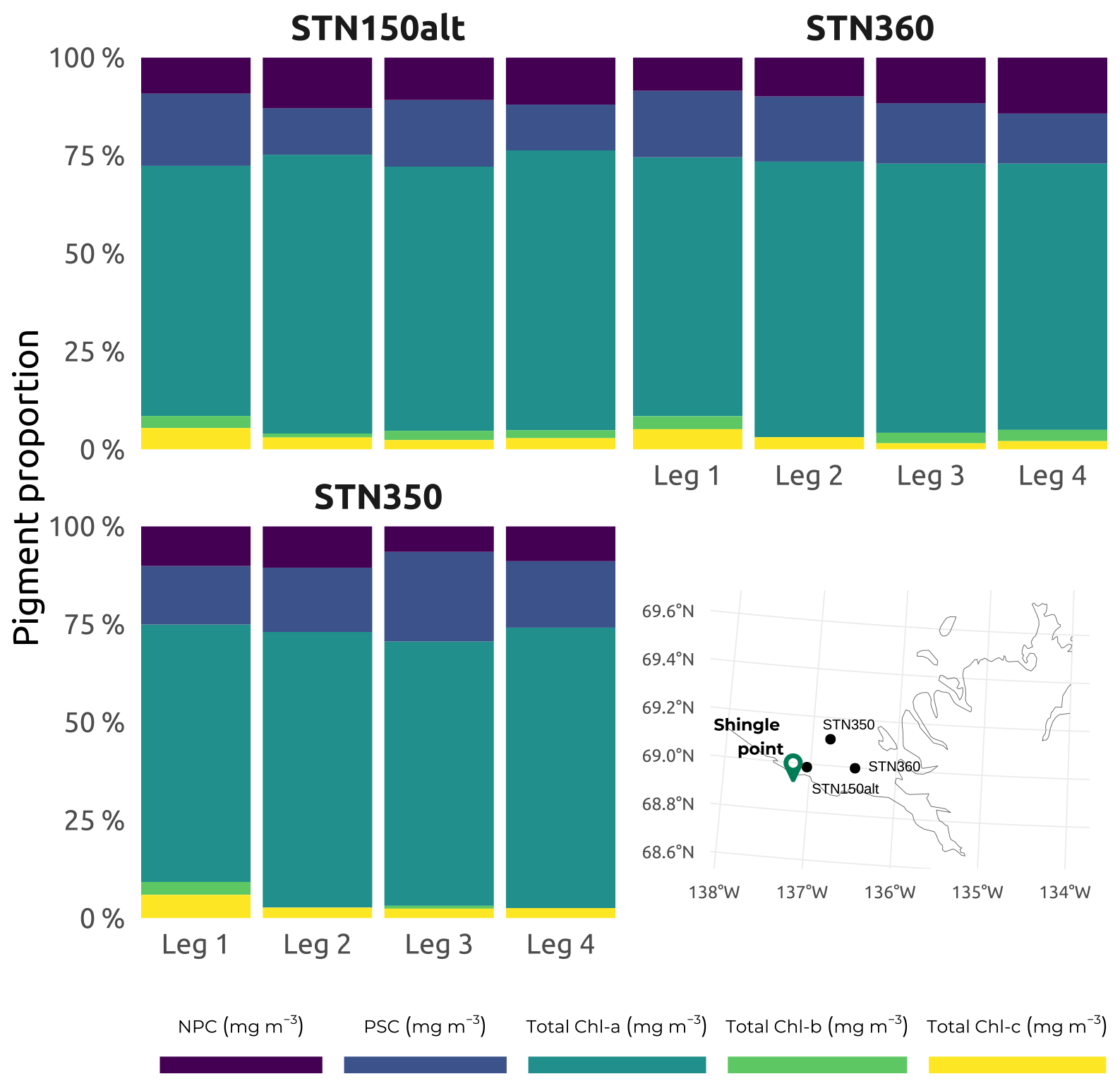
Figure 11 Subset of accessory pigments, classified following Matsuoka et al. (2011), namely non-photosynthetic carotenoids (NPCs) that include zeaxanthin, diadinoxanthin, and alloxanthin and photosynthetic carotenoids (PSCs) that include fucoxanthin, peridinin, 19^′-hexanoyloxyfucoxanthin, and 19^′-butanoyloxyfucoxanthin. Total Chl a, total Chl b, and total Chl c (c₁, c₂, and c₃) are shown for the three selected stations (150ALT, 360, and 350) visited on each of the four WP4 Nunataryuk expeditions (Legs 1, 2, 3, and 4) in 2019. Also included is a map showing the locations of the three stations in the western sector of Mackenzie Bay.

4.3.2 Bacterioplankton abundance and diversity

Samples for the determination of bacterial abundance were prepared immediately at the Aurora Research Institute (Inuvik) upon reception of the water. A volume of 1.5 mL of water was pipetted into a 2 mL Nunc^® cryotube containing 15 µL of 25 % glutaraldehyde. The cryotubes were vortexed for 5 s, allowed to sit at room temperature for 10 min, and then stored in cryoboxes at −80 ^∘C before analysis by flow cytometry with SYBR™ Green I (Thermo Fisher Scientific; Gasol and Del Giorgio, 2000) at the Laboratoire d'Océanographie Microbienne, Banyuls-sur-Mer, France. The mean coefficient of variation for this quantification was below to 5 % (n=3). Median concentrations of bacterial cells (Fig. 10b) were lowest during Leg 1 and highest during the summer months (Legs 2 and 3).

Molecular samples for the determination of bacterial RNA–DNA were processed as follows. Volumes of 1.5 L of water were collected in clean, prerinsed Corning pyrex media storage bottles. Glass filtration systems or plastic magnetic filter funnels of 47 mm diameter were cleaned with ELIMINase^® and rinsed with Milli-Q water. A total of 10 mL of water was run through the filtration unit to condition it for each new sample; this procedure was repeated three times. Then, a 0.2 µm polyethersulfone membrane was placed on the filtration head using tweezers cleaned with ELIMINase^® and ethanol. Then, 500 mL of water was filtered through the glass system, and the filter was then immediately placed into a cryovial. A RNAlater buffer was added to the cryovial to submerge the filter completely. The filtration process was conducted in triplicate to obtain three separate filters for later analysis. Great care was taken during these procedures, including the use of lab coats, hair nets, and powder-free gloves cleaned frequently with ethanol. The cryovials were stored in −80 ^∘C freezers, shipped in liquid-nitrogen-preconditioned dry shippers, and stored again in −80 ^∘C freezers until their analysis at the Institut national de la recherche scientifique in Quebec city.

DNA extraction was performed using a DNeasy PowerSoil Pro Kit (Qiagen), following the instructions provided by the manufacturer, and DNA extracts were quantified on a Qubit fluorometer (the mean coefficient of variation for such quantification was about 30 %). Extracts were sent to the Integrated Microbiome Resource (Dalhousie University, Halifax, Canada), where library preparation, multiplexing, and sequencing were performed for bacteria. The sequencing targeted the V4–V5 regions of the 16S rRNA gene using the 515FB (5^′-GTGYCAGCMGCCGCGGTAA-3^′) and 926R (5^′-CCGYCAATTYMTTTRAGTTT-3^′) primer sets (Parada et al., 2016; Walters et al., 2016). Sequencing was performed on an Illumina MiSeq platform, and the sequences were then analyzed using the DADA2 pipeline v1.16 (Callahan et al., 2016) in R v4.1.2 (R Core Team, 2022). Taxonomy assignment was performed up to the genus level, with the SILVA reference database v138 (Quast et al., 2012). Details on the amplicon sequence variants (ASVs) of bacterial communities are given in Table 2.

For bacterial isolation, samples (0.5 mL) were placed in cryotubes containing 500 µL of 70 % sterile glycerol and stored at −80 ^∘C before isolation at the laboratory. After thawing, 100 µL of each sample was spread in triplicate on R2A Agar plates adjusted to the salinity of the samples, and the petri dishes were incubated in the dark at 10 ^∘C to allow the development of aerobic heterotrophic psychrotolerant marine bacteria. At regular intervals (1, 2, and 3 weeks), the colonies were counted and categorized based on their morphological characteristics (morphotypes). Representatives of each morphotype were selected for isolation by repeated streaking. After isolation and purification, each strain was cultivated in R2A Broth medium (Neogen Corporation) at 10 ^∘C under agitation and darkness before DNA extraction using the Wizard^® Genomic DNA Purification Kit (Promega Corporation) and partial sequencing of the 16S rRNA using a Sanger 16 capillary sequencer AB3130XL (Applied Biosystems) to identify the bacterial strains (Tisserand et al., 2020). A total of 85 bacterial strains were isolated and identified.

4.3.3 Fungal abundance and diversity

Following DNA extraction (see above), fungal abundance was evaluated by a real-time quantitative polymerase chain reaction (qPCR) using the primer set FungiQuant-F (5^′-GGRAAACTCCACCAGGTCCAG-3^′) and FungiQuant-R (5^′-GSWCTATCCCCAKCACGA-3^′; Liu et al., 2012) and following the protocol described in Maza-Márquez et al. (2020). The mean coefficient of variation for such a quantification was about 25 % (n=3). Amplicon sequence variants (ASVs) of fungal communities were determined by Illumina MiSeq sequencing and metabarcoding analysis. After DNA extraction (see above), an amplification of the fungal internal transcribed spacer 2 (ITS2) region, library preparation, multiplexing, and sequencing were performed by LGC Genomics GmbH (Berlin, Germany). The fungal ITS2 region was amplified using the primer pair fITS7 (5^′-GTGARTCATCGAATCTTTG-3^′) and ITS4 (5^′-TCCTCCGCTTATTGATATGC-3^′; Shinohara et al., 2021). Sequence processing was performed following the R package DADA2 pipeline version 1.16 (Callahan et al., 2016) with R software (version 4.0.5; R Core Team, 2014). Taxonomic assignment was performed using UNITE (version 8.3; Nilsson et al., 2019) databases. Metadata related to fungal abundance and diversity can be found in Table 2. DNA sequences were deposited in the National Center for Biotechnology Information (NCBI) Sequence Read Archive (SRA) under accession number PRJNA822885.

4.3.4 Microbial respiration

Microbial respiration rates (see the metadata in Table 2) were derived from continuous dissolved oxygen (O₂) measurements using a SensorDish^® Reader (SDR; PreSens, Germany) optical sensing system equipped with 24 glass vials of 5 mL containing non-invasive O₂ sensors (OxoDish^®). The sensor vials were top-filled with sample water, then sealed without headspace or bubbles, and inserted into the SDR plate. The entire setup was placed in an incubator at a constant temperature of 10 ^∘C. Dissolved O₂ concentrations were derived from 10 min averages of quenched fluorescence measurements taken every minute over a period of 10 h. Linear regression analysis was performed on the dissolved O₂ concentration data from each vial to determine microbial respiration ($\mathrm{\mu }\mathrm{mol}{\mathrm{O}}_{\mathrm{2}}{\mathrm{L}}^{-\mathrm{1}}{\mathrm{h}}^{-\mathrm{1}}$). The mean coefficient of variation for this measurement was about 20 % (n=3).

4.4 Supplementary data

During the extensive 2019 Nunataryuk WP4 field campaign, the opportunity for additional sampling arose, and a subset of variables (e.g., cations, anions, sulfides, and major and rare Earth elements) were measured from sediments, in addition to pore water, extracted from the western and eastern sectors of the Mackenzie Delta region (see Fig. 12 and the metadata presented in Table 2). Additionally, two sites near Tuktoyaktuk (Tuktoyaktuk Island and Peninsula Point in the Pingo Canadian Landmark; see Fig. 13) were sampled between 20 July and 5 August 2019 for massive ice, groundwater, and meltwater on permafrost slumps. These samples served to conduct several analyses, including the abundance of naturally occurring stable and radio isotopes, dissolved total iron (Fe_tot), DOC, and CDOM fluorescence measurements (Table 2). An exhaustive list of variables is presented in Table 2, along with contact information of principal investigators associated with each measured variable or estimated parameter. Full datasets associated with the Nunataryuk WP4 field campaigns can be found in Juhls et al. (2021).

4.4.1 Sediment and pore water

Sediment cores were retrieved using an UWITEC gravity corer fitted with predrilled liners, with holes every 1 cm for pore water (PW) retrieval. The corer was deployed from a tripod through ice holes during Leg 1 (Fig. E1) and from a davit secured on small boats during Leg 4 (Block et al., 2019). Overall, 5 and 10 stations were sampled during Leg 1 and Leg 4, respectively (Fig. 12). Sediment cores from the western region (Mackenzie and Shallow bays) were brought back for processing in the laboratories of the Aurora Research Institute (Inuvik), while processing of the cores sampled in the eastern region (Kugmallit and Kittigazuit bays) was conducted in converted workspaces at the Tuktoyaktuk Learning Center. Pore water was sampled using rhizons (Rhizosphere Research Products) with 0.2 µm polyethersulfone (PES; Seeberg-Elverfeldt et al., 2005). The PW was divided into four different subsamples in vials prepared for specific analysis. Acid-washed high-density polyethylene (HDPE) centrifuge tubes containing 200 µL of ultrapure HNO₃ were used for cations. Amber glass vials (4 mL) with polytetrafluoroethylene (PTFE)-lined caps were used for the analysis of DOC, after being acid-washed in hydrochloric acid (HCl) 10 % and burned at 500 ^∘C overnight. Rinsed polypropylene gas chromatography vials were used to preserve anions for later analysis. Last, nitrogen-filled amber vials amended with 100 µL of 10 % zinc acetate solution were used to preserve dissolved sulfide.

Cations were analyzed with Agilent 8800 ICP-QQQ-MS, while DOC analysis was conducted on a Shimadzu total organic carbon analyzer, TOC-VCPH (Neweshy et al., 2022). Sulfides were analyzed using a HORIBA Aqualog^®, and the analysis of anions will be conducted by Dionex Integrion HPIC (high-performance ion chromatography; Couture et al., 2016). To ensure instrumental accuracy, certified reference materials were used when available. The accuracy and precision of each method was evaluated with the results from these analyses. When no certified reference materials were available, then control samples were prepared by another scientist to ensure that no systematic errors were applied to samples and that the calibration curves were accurate. When control samples were used, measurements were taken 10 times, and a variation of 10 % was accepted.

The sediment cores were sliced every 1 cm. The subsamples were placed in Falcon cups and kept frozen until treatment. The samples were then freeze-dried and homogenized with an agate pestle and mortar. Ground, freeze-dried sediment was mineralized using ultrapure nitric and hydrochloric acids using a microwave (Mars5 EasyPrep Microwave vessels). Results were validated against MESS-4 certified reference material (National Research Council Canada). The mineralization protocol used is based on Ma et al. (2019). Major (Fe, Ca, Na, Mg, Mn, and K) and rare Earth elements (REEs) in the sediment were analyzed using a Thermo Fisher Scientific iCAP 7400 ICP-OES and an Agilent 8800 ICP-QQQ-MS, respectively.

For cation pore water analysis, SLRS-6 from the National Research Council Canada (Ottawa, Canada) certified reference material was used to validate the method (n=3). The values were always within 12 % of certified values. The precision, expressed as the coefficient of variation in replicates analysis was under 10 % for most analytes.

For cation sediment analysis, MESS-4 from the National Research Council Canada (Ottawa, Canada) certified reference material was used to validate the method (n=9). The values were always within 8 % of certified values. The precision, expressed as the coefficient of variation in replicates analysis, was under 10 % for all analytes.

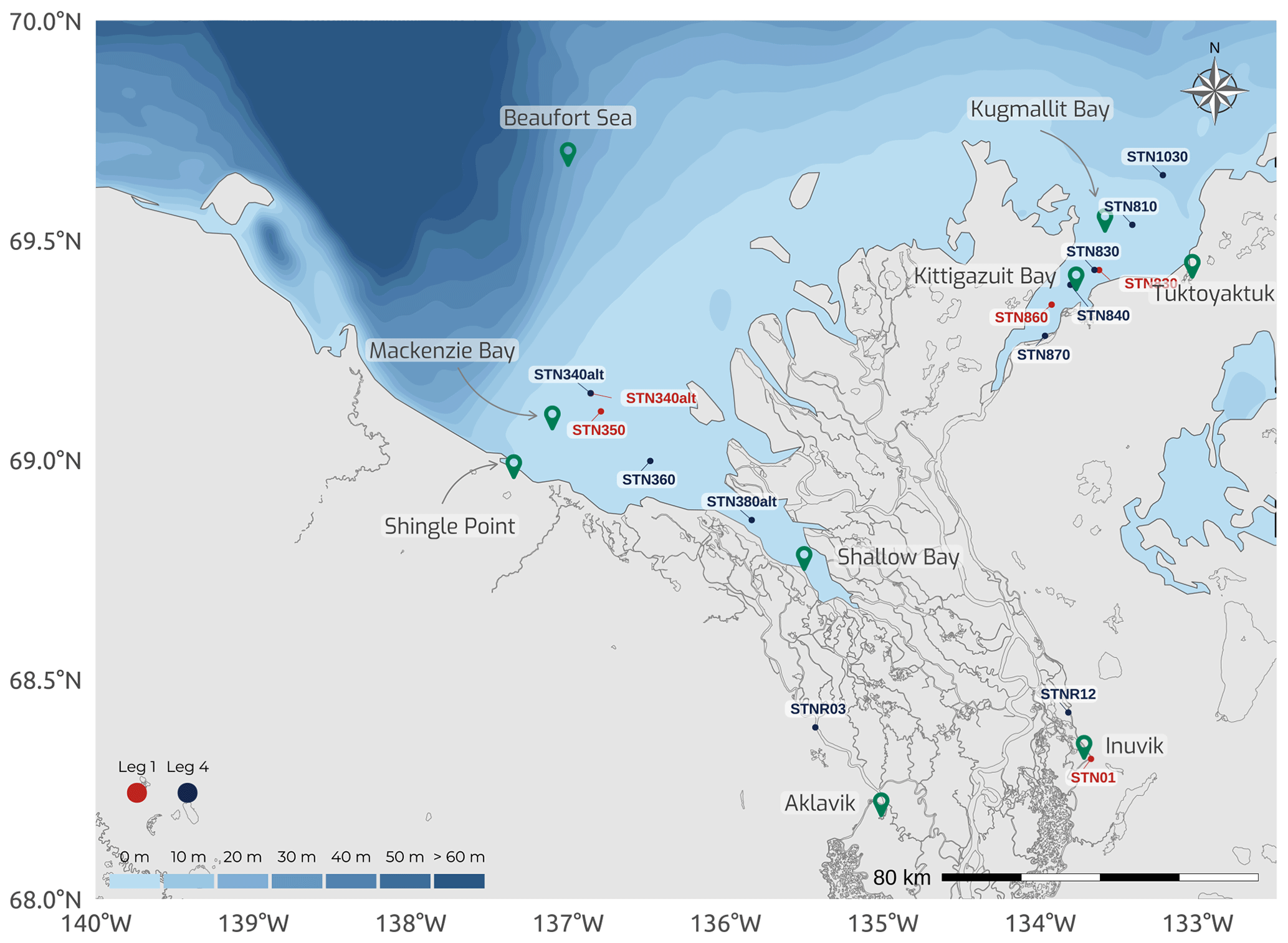
Figure 12 Map of the Mackenzie Delta region (Inuvialuit Settlement Region, Northwest Territories, Canada), with bathymetric features of the coastal waters of the southern Beaufort Sea, showing the locations for the sediment and pore water sampling during two legs of the 2019 WP4 Nunataryuk field expeditions (Legs 1 and 4).

4.4.2 Groundwater

Two sites near Tuktoyaktuk were investigated between 20 July and 5 August 2019 (Tuktoyaktuk Island, 69.4557^∘ N, 133.0039^∘ W; Peninsula Point in the Pingo Canadian Landmark, 69.4552^∘ N, 133.0069^∘ W; see Fig. 13). Massive ice, groundwater, and meltwater samples were collected on permafrost slumps. Seawater samples were also collected in front of each study site at 0.5, 1, 1.5, and 2 km from the coastline.

Radon, radium, and stable isotopes of water (δ¹⁸O; δ²H)

Naturally occurring radon (²²²Rn; half-life of 3.8 d) and radium (²²³Ra, ²²⁴Ra, ²²⁶Ra, and ²²⁸Ra; half-lives of 11.4 d, 3.6 d, 1600 years, and 5.8 years, respectively) isotopes in the environment are efficient geochemical tracers to map and quantify submarine groundwater discharge in nearshore waters. Groundwater is defined as water of any salinity that has circulated through the coastal aquifer (Moore, 1999), and groundwater is here synonymous with pore water. Massive ice, groundwater, and meltwater samples were collected on permafrost slumps. Seawater samples were also collected in front of each study site at 0.5, 1, 1.5, and 2 km from the coastline. Massive ice samples were collected and immediately stored in airtight buckets to limit radon loss. They were then kept at room temperature in the laboratory until they had melted completely. Groundwater, meltwater, and seawater were collected using a peristaltic or a submersible pump. Water was continuously pumped at an approximate flow rate varying from 0.2 to 0.8 L min⁻¹ through a Teflon tube into an inline flow cell where temperature, practical salinity, and oxygen saturation were monitored with a daily calibrated multiparametric probe (YSI 600QS). For radon, 2 L of water was sampled in plastic bottles that were tightly sealed. Within the next 12 h, analyses were carried out, as described in Chaillou et al. (2018). Briefly, the water was bubbled to allow ²²²Rn degassing, and the equilibrated air flowed through Drierite desiccant to a radon-in-air detector (RAD7; DURRIDGE Company, Inc.). The air volume of the closed-loop and water volume of the bottle were known and constant over the measurement. The air recirculated through the water and continuously extracted the radon until a state of equilibrium developed. Radon-in-water activities were finally corrected by temperature and humidity and by radon decay that took place between sampling and analysis. Analytical uncertainties were less than 10 % (2σ).

Samples for radium were filtered through a 1 µm Hytrex cartridge (seawater) or a 0.45 µm Pall Corporation high-capacity capsule filter (groundwater and melted ice) to remove suspended sediment and then through an acrylic fiber coated in manganese oxide (MnO₂), which quantitatively scavenges Ra (Reid et al., 1979). Fibers were thoroughly rinsed with Ra-free water to remove any additional particles before analysis. Sample volumes ranged from 1–20 L for groundwater and thawed ice and up to 120 L for seawater. The short-lived ²²⁴Ra and ²²³Ra isotopes were measured using a radium delayed coincidence counter (RaDeCC) system (Moore and Arnold, 1996) within 3 d of sample collection. Fibers were reanalyzed after 4 weeks and after 2 months to determine the activities of ²²⁴Ra and ²²³Ra supported by parent isotopes ²²⁸Th (half-life of 1.91 years) and ²²⁷Ac (half-life of 21.8 years), respectively. Activities of ²²⁴Ra and ²²³Ra reported in Table 2 are the activities in excess of the parent isotopes (unsupported activities). Following RaDeCC analyses, fibers were sealed in an airtight housing for 3 weeks to allow ²²²Rn to reach equilibrium with ²²⁶Ra. The activities of ²²⁶Ra were then determined via ²²²Rn emanation and scintillation counting, following the methods described in Key et al. (1979). The efficiency of RaDeCC and scintillation counting was determined using MnO₂-coated fibers spiked with known activities of radium.

In addition to radon and radium isotopes in water, the mineral-bound ²²⁶Ra activity of sediments was determined on four (4) sediment samples (two coastal permafrost cliff and two surficial Holocene inshore) collected at each site. These measurements were done as a first attempt to monitor the activity of ²²⁶Ra-supported ²²²Rn in groundwater. A total of 15 g of sediment samples were dried, crushed, and sealed in vials fitted for a high-purity Germanium gamma-ray spectrometer (ORTEC^® GMX50) at the ISMER (l'Institut des sciences de la mer de Rimouski) laboratory (University of Quebec at Rimouski (UQAR), Rimouski, Canada). They were left in sealed vials for at least 23 d to ensure radioactive re-equilibration between the ²²⁶Ra and the short-lived daughters of the ²³⁸U series (Zielinski et al., 2001). Counting time was fixed at 4 to 5 d to provide adequate counts for the peaks of ²¹⁴Pb (using the 295.2 and 352 keV) and ²¹⁴Bi (609 keV) peaks. The counting error was <10 %. Disintegrations per minute, (dpm g⁻¹), were converted to becquerel per cubic meter (Bq m⁻³) of wet sediment.

Unfiltered water samples for the determination of stable water isotopes were collected in 30 mL HDPE vials free of any chemicals, sealed tightly, and stored in the dark at 4 ^∘C. Stable isotopes of water (δ¹⁸O, δ²H) were analyzed by elemental analysis–isotope ratio mass spectrometry (EA-IRMS) at the Geotop laboratory (Université du Québec à Montréal (UQAM), Montreal, Canada). The precision was ±0.05 ‰ and ±1 ‰ (at the 1σ level) for δ¹⁸O and δ²H, respectively. Isotopic analyses are reported as compared to the international Vienna Standard Mean Ocean Water (VSMOW). Reference materials were used throughout the isotopic water analyses to ensure high-quality data.

Dissolved total iron (Fe_tot), DOC, and CDOM fluorescence measurements

Duplicate dissolved organic carbon (DOC) samples were collected at the outlet of a Teflon tube using acid-cleaned 60 mL polypropylene syringes and were directly filtered through combusted 0.7 µm glass-fiber filters. The filtered samples were acidified using high-purity HCl (37 %) to pH <2 in combusted borosilicate tubes with PTFE caps after being acid-washed in hydrochloric acid (HCl) 1 %, burned at 500 ^∘C overnight, and stored in the dark at 4 ^∘C until analysis. DOC was analyzed a few weeks post-collection using a total organic carbon analyzer (TOC-VCPN, Shimadzu), based on the method of Wurl and Sin (2009), and combined with a total nitrogen measuring unit (TNM-1, Shimadzu) at ISMER (UQAR, Rimouski, Canada). The analytical uncertainties were less than 2 %, and the detection limit was 0.05 mg L⁻¹. Fresh acidified deionized water (blank) and a standard solution (1.1±0.03 mg C L⁻¹) were frequently analyzed during measurements to ensure the stability of the instrument's performance.

Figure 13 Examples of excitation–emission matrices (EEMs) obtained for seawater samples (stations 15, 17, and 18), beach groundwater (station 7), and thawed permafrost and massive ice (station 4) collected in Tuktoyaktuk Island site during Leg 3 of the 2019 WP4 Nunataryuk field expeditions. EEMs are all corrected for the Raman and Rayleigh scattering and the inner-filter effect. Note that the intensity scale is the same for each sample. The shapefiles for the Tuktoyaktuk area were from https://www.geogratis.gc.ca/ (last access: 3 February 2023).

Water samples for total dissolved Fe and CDOM were pumped through a Teflon tube and directly filtered using a Millipore Opticap^® XL 4 capsule with a Durapore™ membrane (0.22 µm porosity) connected to the outlet of the tube. Total dissolved Fe (Fe_tot) samples were stored in 15 mL Falcon™ tubes, acidified to pH <2 with an ultratrace parts per billion (ppb)-grade HCl (37 %) solution, and stored at 4 ^∘C prior to total dissolved Fe analysis. Fe_tot was measured using the Ferrozine method modified by Viollier et al. (2000), with a detection limit of 0.3 µM. Measurements were done using a GENESYS 20 spectrophotometer (Thermo Fisher Scientific), using a quartz cuvette with a pathlength of 1 cm. CDOM samples were stored in acid-cleaned 15 mL glass tubes in the dark at 4 ^∘C prior to analysis. Absorbance and fluorescence of CDOM were measured simultaneously. Before optical analysis, samples were allowed to equilibrate at room temperature (20 ^∘C). CDOM absorbance in the UV-visible spectrum was measured using a LAMBDA 850 UV-VIS spectrophotometer (PerkinElmer) fitted with two 1 cm pathlength quartz cuvettes, with one used for the reference and one for the sample. Measurements were taken from 220 to 800 nm at 1 nm intervals, with a scanning speed of 100 nm min⁻¹. Note that the method used to measure CDOM and DOC for these samples differs from samples described in Sect. 4.1.2 and 4.1.3. Fresh Milli-Q water was used as blanks and references during the analysis. The reference water was refreshed every 30 min. Before each analysis, the quartz cuvette was flushed first with 5 % HCl, then with deionized water, and finally with the sample. Absorbance metrics were then extracted from the different scans. Concomitantly, CDOM fluorescence was measured using a Varian Cary Eclipse fluorometer and a 1 cm pathlength quartz cuvette. Emission wavelengths (λ_Em) ranged from 230 to 600 nm and excitation wavelengths (λ_Ex) from 220 to 450 nm. When the absorbance was higher than 0.3 at 254 nm, the sample was diluted to avoid saturating the fluorometer (Miller and McKnight, 2010). Fresh deionized water was used as a blank, and absorbance measurements of the samples were used to correct the fluorescence data for inner-filter effects. All data were corrected for the Raman and Rayleigh effects, using daily fresh deionized water signals, and for the inner-filter effect, using absorbance spectra. Moreover, because the low concentrations of Fe_tot result in low total Fe:DOC molar ratios, of the order of 10⁻², this suggested that the Fe effect on the absorbance and fluorescence of CDOM was negligible (Poulin et al., 2014). Therefore, no Fe effect correction was applied to the DOM concentration, absorbance, and fluorescence. The collected data were then described as excitation–emission matrices (EEMs), and different absorbance and fluorescence metrics were calculated (Fig. 13). Briefly, EEM and fluorescent metrics were produced using the eemR package proposed by Massicotte (2019) for R software. Prior to extraction of the fluorescent DOM metrics, a Raman calibration was performed for each EEM to remove the dependence of the fluorescence intensities on the measurement equipment, as proposed by Lawaetz and Stedmon (2009). This database was completed by 50 more samples collected in the same region in summer 2021 (see Flamand et al., 2023, for details). Fluorescence spectroscopy can be indicative of the origin of the DOM pool. In this dataset, fluorescence spectroscopy was successfully used to determine the origin of the DOM pool. Fluorescence occurring at low excitation–emission wavelengths was associated with protein-like material originating from autochthonous production, whereas fluorescence happening at higher wavelengths was associated with humic-like material of higher molecular weight derived from terrestrial sources (Coble, 1996; Murphy et al., 2008). In Fig. 13, different DOM fluorescence signatures can be observed across stations distributed along a north–south transect near Tuktoyaktuk. Strong signals of protein-like and humic-like fluorescence can be observed at seawater stations 17 and 18, as well as at the beach groundwater station 7, which represent stations characterized by a mixture of FDOM. In contrast, there are no obvious signals of in-situ-derived FDOM at station 4, which was derived from the thawing of massive ice.

Dissolved inorganic carbon (DIC) and methane (CH₄)

Water samples for dissolved inorganic carbon (DIC or $\sum {\mathrm{CO}}_{\mathrm{2}}={\mathrm{CO}}_{\mathrm{2}}+{\mathrm{HCO}}_{\mathrm{3}}^{-}+{\mathrm{CO}}_{\mathrm{3}}^{\mathrm{2}-}$; also called total carbonate) and methane were pumped and stored in 120 mL borosilicate glass bottles hermetically closed with a Teflon rubber crimped with an aluminum ferrule. A total solution of 0.2 mL of HgCl₂ (7 mg L⁻¹) was added into each bottle. The DIC concentration of samples were determined using a Apollo SciTech DIC analyzer. After reaching thermal equilibration at 25 ^∘C, duplicates of 30 mL of the sample were injected into the instrument's reactor, where they were acidified with 10 % H₃PO₄. The CO₂ formed was then carried to a LI-COR infrared analyzer by a stream of pure nitrogen. A calibration curve was constructed using Na₂CO₃ solutions, and the accuracy of the measurements was verified using the Dickson batch 122 standard. Reproducibility was typically of the order of 0.2 %. Methane (CH₄) concentrations were determined by a Peak Performer gas chromatography with flame ionization detection (GC-FID; 2 mL sample loop; Peak Laboratories, LLC, USA), based on the static headspace method reported by Zhang and Xie (2015). The samples were transferred into a 50 mL glass syringe, and 5 mL of CH₄-free N₂ was introduced to obtain a 1:10 gas : water ratio. The syringe was vigorously shaken for 4 min, and the equilibrated headspace gas was injected into the GC-FID for CH₄ quantification. The methane concentrations in the headspace were calculated using the respective volumes of water and headspace in the vial and the solubility coefficient of methane of Yamamoto et al. (1976) as a function of temperature and salinity. The analyzer was calibrated with a methane standard of 4.94 ppm by volume (ppmv; Air Liquide), traceable to the National Institute of Standards and Technology, and the precision of the technique was ±4 % (at 5 nmol L⁻¹).

5 Code and data availability

The raw data and metadata provided are hosted on VALERIA (a Laval University user-specific repository), and final aligned and cleaned datasets are available on Pangaea (see Table 2; Juhls et al., 2021; https://doi.org/10.1594/PANGAEA.937587). Detailed metadata are associated with each file, including the principal investigator's contact information. For specific questions, please contact the principal investigator associated with the data (see Table 2). The code used to process the figures and tables is publicly available (https://doi.org/10.5281/zenodo.7603079; Massicotte, 2023) under the MIT license.

6 Conclusions

Fundamental physical, optical, chemical, and biological properties associated with reservoirs and fluxes of OMt were acquired, measured, and processed during four WP4 Nunataryuk field campaigns in the Mackenzie Delta region and adjacent coastal waters of the Beaufort Sea (ISR, Northwest Territories, Canada). A subset of the broad dataset has been presented and described here. A full list of variables measured during the field expeditions can be found in Table 2, including authorship information for these datasets. Several of the datasets have been fed into Pangaea data publisher for Earth and environmental science, in order to promote the principles of the International Council for Science – World Data System (ICS-WDS). As far as we know, the data gathered and currently included in this paper are unparalleled in the breadth of their spatiotemporal coverage of a fluvial-to-marine transitional region in the Arctic. The scope of the dataset presented here offers contingencies towards its further exploitation in research.

Appendix A

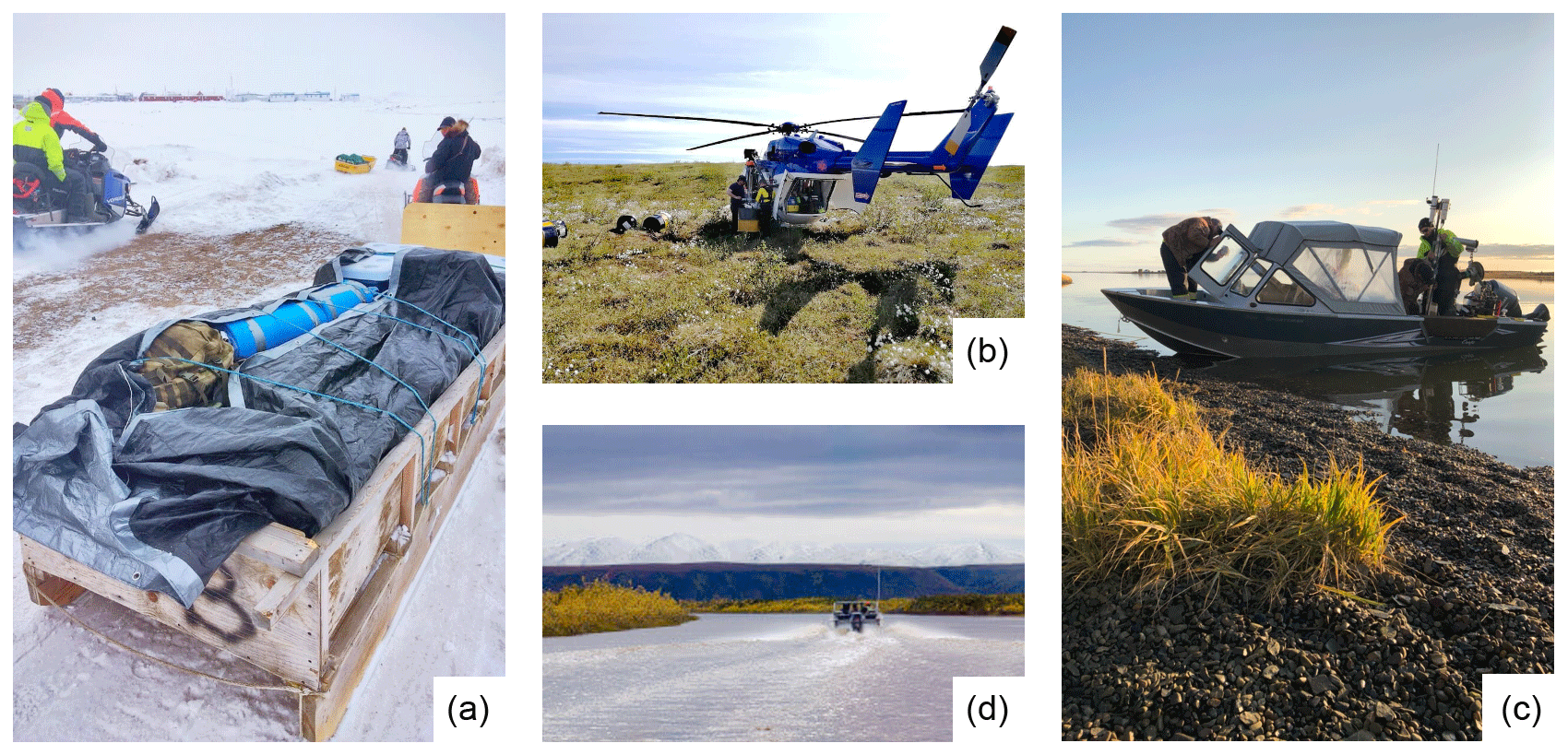
Figure A1 Vehicles used to access sampling regions during the Nunataryuk WP4 field campaign. (a) Snowmobiles during Leg 1 (picture credit: Martine Lizotte). (b) Helicopter during Leg 2 (picture credit: Bennet Juhls). (c) Small boats during Leg 3 (picture credit: Joannie Ferland). (d) Small boats during Leg 4 (picture credit: Laurent Oziel).

Appendix B

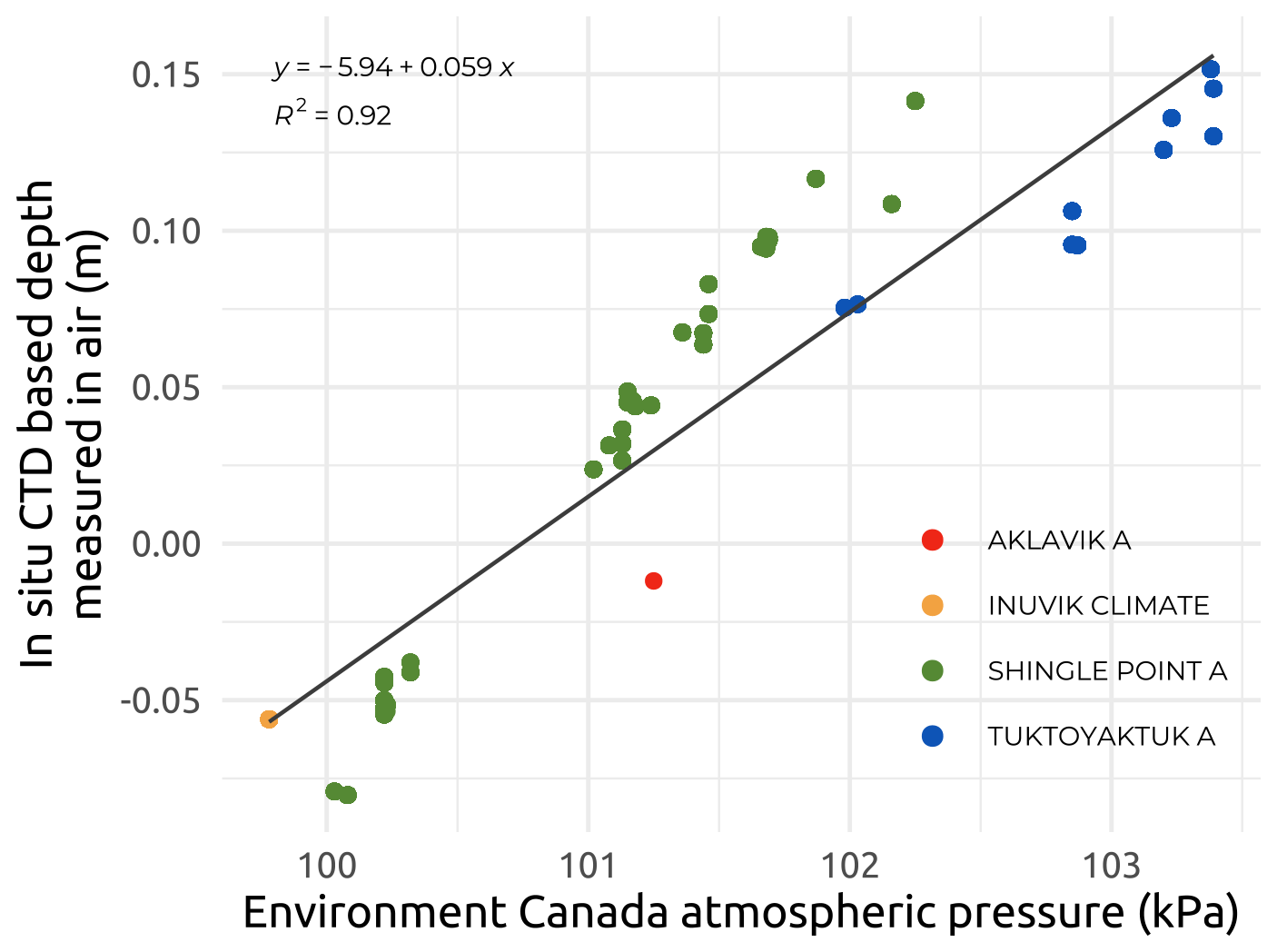
Figure B1 Depth tare correction of in situ, CTD-based depth measured in air against Environment and Climate Change Canada values of atmospheric pressure with linear model fit.

Appendix C

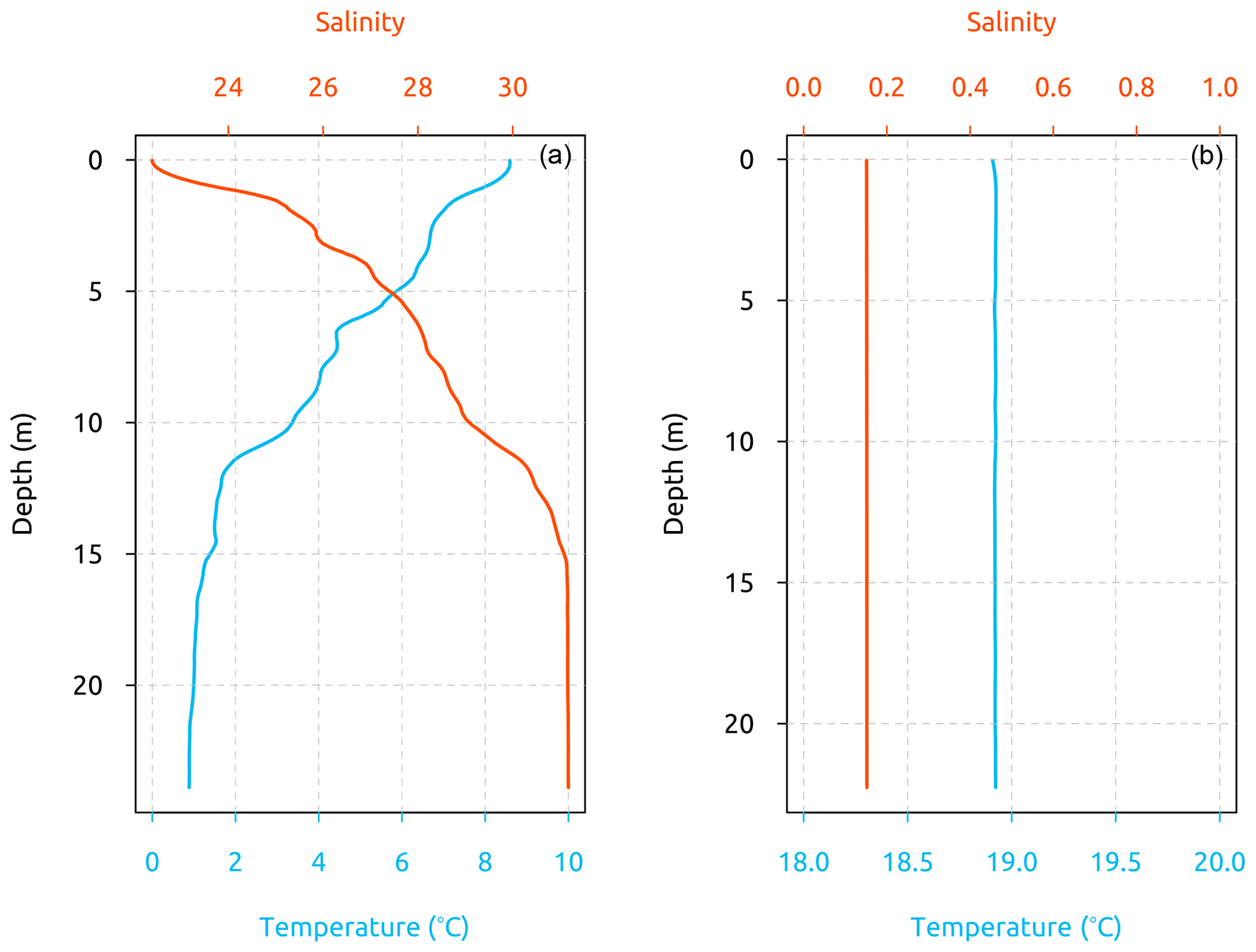
Figure C1 Two examples of vertical profiles of temperature (^∘C) and salinity. (a) STN125 on 28 July 2019. (b) STNR09 on 29 July 2019. Note the difference in scales for temperature and salinity between the panels.

Appendix D

The ranges of light absorption (a) and scattering (b) coefficients encountered in the Mackenzie River delta zone greatly exceeded the ones considered by Gordon and Ding (1992) when developing a well-known correction for self-shading of in-water radiometric measurements. Values of light absorption coefficients (a) were obtained either from a partial processing of the optical frame data (see Sect. 4.1.9) or from absorption coefficients of CDOM, as well as particulate absorption coefficient values (see Sect. 4.1.2 and 4.1.7). The scattering coefficient (b) was estimated from a Beaufort-Sea-specific relationship published in Doxaran et al. (2012). Also, the Monte Carlo code SimulO (Leymarie et al., 2010; Doxaran et al., 2016; Voss et al., 2021) was used here to estimate and correct for the self-shading effects on in-water upwelling radiance measurements carried out using a Biospherical C-OPS radiometer deployed on the Ice Pro profiling platform. The exact dimensions of the Ice Pro platform (a cylinder of 11.5 cm radius and 23.5 cm length) and radiometer (a cylinder of 3.5 cm radius and 36.9 cm length) were used as inputs in SimulO. The very wide ranges of a and b coefficients (up to 12 and 100 m⁻¹, respectively) were considered, together with two particle scattering-phase functions, namely Fournier–Forand, with backscattering ratios of 1.83 % and 4 % (FF183 and FF400). Black- and blue-sky conditions were imposed, with solar zenith angles spanning from 4 to 8^∘. The upwelling radiance signal near the surface (0.5 m) was computed using SimulO successively without, and then with, the sensor and Ice Pro platform. The difference observed, in percent, was assumed to be the associated near-surface self-shading induced by the profiling system (see Fig. D1), as described in detail in Voss et al. (2021).

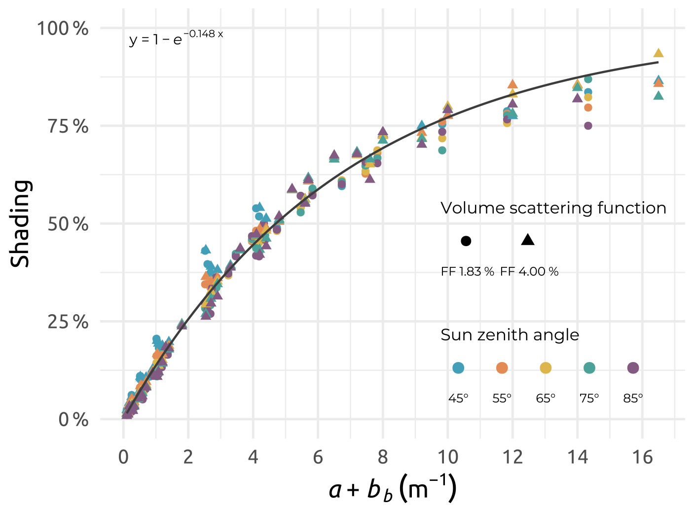
Figure D1 Relationship established between the self-shading computed using SimulO and the sum a+b_b, with a and b_b (in m⁻¹) as the absorption and backscattering coefficients, respectively, for the two particle volume scattering functions (FF 1.83 % and FF 4.00 %) and five solar zenith angles considered.

Within the limited ranges of a and b considered by Gordon and Ding (1992), a good agreement was observed between the shading simulated with the two models, with the self-shading being, as a first approximation, a function of the absorption coefficient (not shown). Considering the whole ranges of a and b coefficients, the self-shading estimated using SimulO was no longer a simple function of the absorption coefficient. Additionally, considering the influence of in-water light backscattering, a function of the form $y=\mathrm{1}-e^{-\mathit{\alpha }(a+b_{\mathrm{b}})}$ was fitted through the simulated Ice Pro plus radiometer self-shading factors, with b_b (in m⁻¹) being the total backscattering coefficient (Fig. D1). This function was used to correct the measured upwelling radiance measurements at zero depth for self-shading effects.

Appendix E

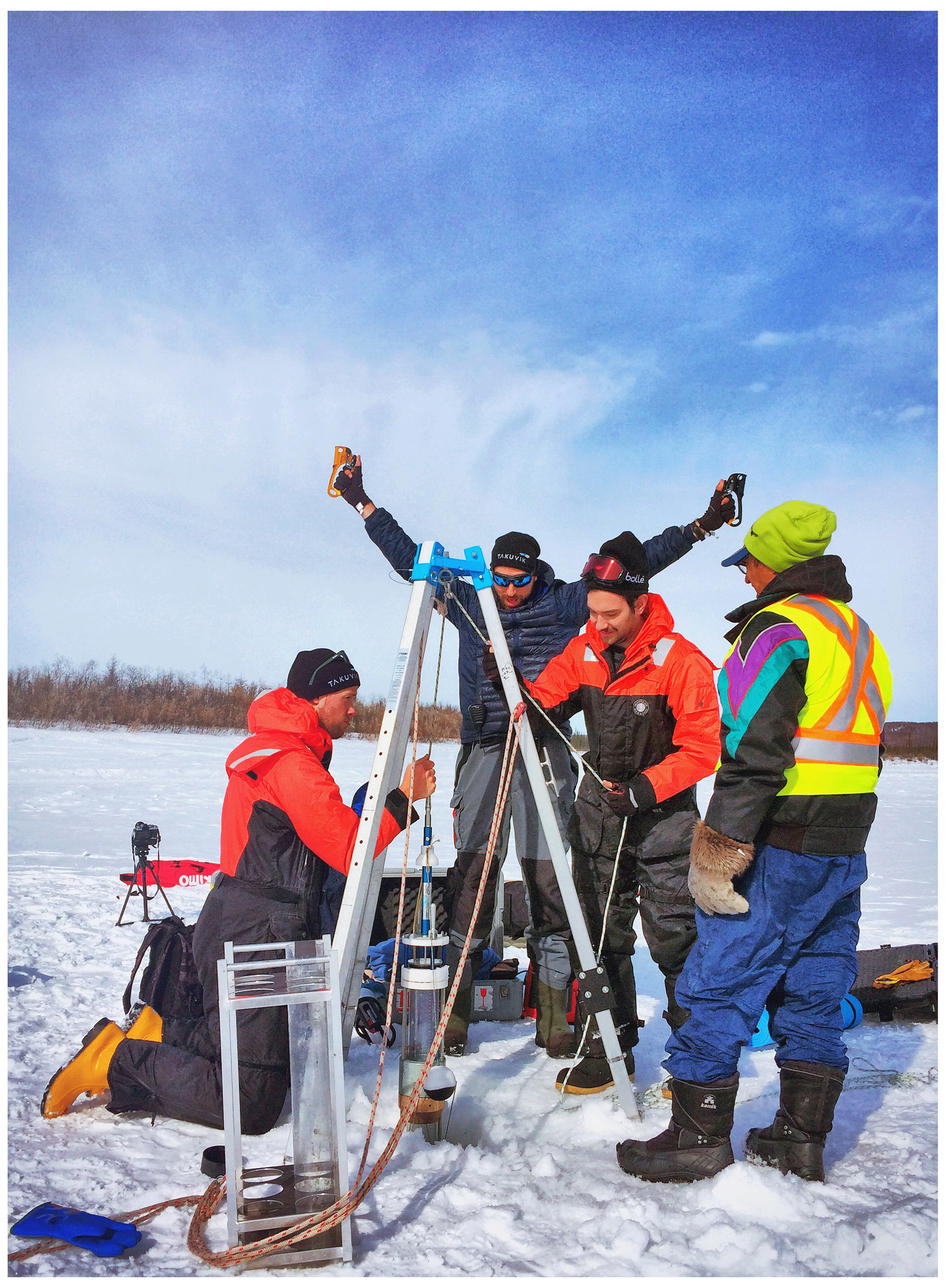
Figure E1 Picture taken during Leg 1 of the Nunataryuk expeditions showing the setup of the tripod and corer (picture credit: Martine Lizotte).