the Creative Commons Attribution 4.0 License.
the Creative Commons Attribution 4.0 License.
 | 31 Mar 2023
A 29-year time series of annual 300 m resolution plant-functional-type maps for climate models
Kandice L. Harper
Céline Lamarche
Andrew Hartley
Philippe Peylin
Catherine Ottlé
Vladislav Bastrikov
Rodrigo San Martín
Sylvia I. Bohnenstengel
Grit Kirches
Martin Boettcher
Roman Shevchuk
Carsten Brockmann
Pierre Defourny
The existing medium-resolution land cover time series produced under the European Space Agency's Climate Change Initiative provides 29 years (1992–2020) of annual land cover maps at 300 m resolution, allowing for a detailed study of land change dynamics over the contemporary era. Because models need two-dimensional parameters rather than two-dimensional land cover information, the land cover classes must be converted into model-appropriate plant functional types (PFTs) to apply this time series to Earth system and land surface models. The first-generation cross-walking table that was presented with the land cover product prescribed pixel-level PFT fractional compositions that varied by land cover class but that lacked spatial variability. Here we describe a new ready-to-use data product for climate modelling: spatially explicit annual maps of PFT fractional composition at 300 m resolution for 1992–2020, created by fusing the 300 m medium-resolution land cover product with several existing high-resolution datasets using a globally consistent method. In the resulting data product, which has 14 layers for each of the 29 years, pixel values at 300 m resolution indicate the percentage cover (0 %–100 %) for each of 14 PFTs, with pixel-level PFT composition exhibiting significant intra-class spatial variability at the global scale. We additionally present an updated version of the user tool that allows users to modify the baseline product (e.g. re-mapping, re-projection, PFT conversion, and spatial sub-setting) to meet individual needs. Finally, these new PFT maps have been used in two land surface models – Organising Carbon and Hydrology in Dynamic Ecosystems (ORCHIDEE) and the Joint UK Land Environment Simulator (JULES) – to demonstrate their benefit over the conventional maps based on a generic cross-walking table. Regional changes in the fractions of trees, short vegetation, and bare-soil cover induce changes in surface properties, such as the albedo, leading to significant changes in surface turbulent fluxes, temperature, and vegetation carbon stocks. The dataset is accessible at https://doi.org/10.5285/26a0f46c95ee4c29b5c650b129aab788 (Harper et al., 2023).
- Article
(11537 KB) - Full-text XML
- BibTeX
- EndNote


Terrestrial ecosystems have always been shaped by people who depend on land for their consumption of direct (e.g. food and materials) and indirect (e.g. land for human activities) goods (Vitousek et al., 1986; Foley et al., 2005). Land cover change induces significant biogeochemical and biogeophysical effects on the climate by altering greenhouse gas emissions (e.g. CO2) and the surface energy budget, induced by modified albedo, evapotranspiration, and roughness (Pielke et al., 2011; Mahmood et al., 2014; Pielke, 2005; Brovkin et al., 2006; Dale, 1997; Liu et al., 2017). The fragmented landscapes that result from land cover change also influence surface temperatures, altering clouds and precipitation (Dale, 1997; Perugini et al., 2017; Sampaio et al., 2007). The physical climate changes driven by land cover change can manifest far afield of the surface changes: for example, large areas deforested at the expense of brighter land cover (e.g. cropland expansion) modify albedo (Loarie et al., 2011; Lambin et al., 2001), with the altered energy balance driving changes in monsoon patterns (Feddema et al., 2005; Devaraju et al., 2015).
Anthropogenic activities, driven mainly by economic and population growth (Pachauri et al., 2014), have changed the atmosphere's composition (IPCC, 2022). The land use, land use change, and forestry sectors are estimated to account for net emissions of 4.1±2.6 Gt CO2 yr−1 (1σ uncertainty, period 2011–2020), accounting for 10 % of total anthropogenic CO2 emissions (Friedlingstein et al., 2022). The estimated net CO2 emission uncertainty (±2.6 Gt CO2 yr−1) represents more than 50 % of the 10-year mean emission estimate and is the most uncertain emission component of the global carbon budget (Friedlingstein et al., 2022; Houghton et al., 2012). Various sources contribute to this uncertainty, including differences in the processes implemented in models (Bastos et al., 2020; Houghton et al., 2012; Pitman et al., 2009; McGlynn et al., 2022), including the definition of the fluxes themselves (Pongratz et al., 2014) and the inclusion of management practices (Houghton et al., 2012), the estimates of vegetation biomass density (Houghton, 2005), and estimates of land cover and rates of change (Houghton et al., 2012; Bastos et al., 2021, 2020).
In support of the United Nations Framework Convention on Climate Change (UNFCCC) needs for observations of the climate system, the Global Climate Observing System (GCOS) has identified 54 essential climate variables (ECVs) that critically contribute to improved characterization of the state of the global climate, making predictions of climate changes and performing attribution of the causes of such changes (GCOS, 2016). As a direct response, the European Space Agency (ESA) launched the Climate Change Initiative (CCI) to provide stable, long-term, and consistent satellite climate data records (Hollmann et al., 2013). The CCI thereby provides useful information to monitor the Paris Agreement goal of maintaining the global temperature increase above pre-industrial levels to less than 2 ∘C (UNFCCC, 2016).
Land cover, the observed biophysical cover of the Earth's surface (Di Gregorio and Jansen, 2005; Turner et al., 1993), is an ECV (Sessa, 2008) tackled by the ESA CCI (Plummer et al., 2017). The ESA CCI medium-resolution land cover (MRLC) dataset, operationalized within the EU Copernicus Climate Change Service (C3S) (2016–2020) thanks to strong user endorsement, provides the longest consistent land cover climate data record, with annual maps from 1992 to 2020 at a spatial resolution of 300 m. It describes the land surface in 22 land cover classes according to the standard of the United Nations Land Cover Classification System (UN-LCCS) (Di Gregorio and Jansen, 2005) and 13 land cover change types consistent with the IPCC land categories (Defourny et al., 2023).
The land surface components of global circulation models and global Earth system models (ESMs) play a significant role in quantifying the historical and present-day representations of land use and land cover change impacts on climate. Most land surface models (LSMs) parameterize global vegetation processes (e.g. photosynthesis and evapotranspiration) for a reduced set of globally representative and similarly behaving plant types, referred to as plant functional types (PFTs). PFTs can be related to physiognomy and phenology (Box, 1996), climate (which defines the geographical ranges in which a plant type can grow and reproduce under natural conditions; Box, 1981), and physiological activity (e.g. C3/C4 photosynthetic pathways).
Spectral information acquired by remote-sensing techniques does not allow direct mapping of PFTs. However, land cover map series derived from satellite Earth observations (EOs) are a valuable source of physiognomy (life form and leaf type) and phenology information for inferring the spatial distribution of PFTs. EO-derived land cover maps must be translated (“cross-walked”) into model-specific PFTs, which is typically accomplished using the information provided by the land cover class legend (Jung et al., 2006). Differences in land cover categories, spatial resolutions, and temporal coverage between various land cover products propagate errors to the cross-walked PFT maps and significantly contribute to uncertainties in deriving gross primary production (GPP) and other climate-relevant variables at the regional scale (Poulter et al., 2011). To reduce uncertainty in model ensembles, Poulter et al. (2015) proposed a standardized cross-walking framework that converts each CCI MRLC class into pre-defined PFT fractions relevant for three leading ESMs (JULES-MOHC, ORCHIDEE-LSCE, and JSBACH-MPI, the land component of the Max Planck Institute for Meteorology Earth System models – MPI-M) based on expert knowledge and auxiliary data. This re-classification procedure was implemented in a flexible tool to generate other related PFT schemes required by the modelling community.
Hartley et al. (2017) used the same three ESMs to quantify the impact of uncertainties in (1) the land cover map and (2) the cross-walking procedure on the spatiotemporal patterns of three important land surface variables: GPP, evapotranspiration, and albedo. To disentangle the two sources of uncertainty, the modelling set-up translated the plausible uncertainty ranges of the land cover and cross-walking components into a common biomass scale. The simulations indicated that the uncertainty of the cross-walking procedure contributed slightly more than the uncertainty of the land cover map to the inter-model uncertainty for all three variables.
In a continuation of the ESA CCI contribution to the land cover ECV, this work aims to reduce the uncertainty in the cross-walking component by adding spatial variability to the PFT composition within a land cover class. This work moves beyond fine-tuning the cross-walking approach for specific land cover classes and/or regions and, instead, separately quantifies the PFT fractional composition for each 300 m pixel globally for each year in the time series (1992–2020). The new PFT product is generated by fusing the annual CCI MRLC map series with existing high-resolution auxiliary data products that individually characterize one surface type with high accuracy. The resulting 300 m PFT product is a companion time series of continuous-field PFT fractions that is consistent with the existing CCI MRLC map series. The global PFT product has an annual resolution, covering 1992–2020, and indicates the specific percentage cover of 14 PFTs for each pixel at 300 m resolution. The set of 14 PFTs represented in the product includes the full set of 13 PFTs initially developed by Poulter et al. (2015) complemented with a new built-up surface type. The full set of PFTs includes bare soil, built, water, snow and ice, natural grasses, managed grasses (i.e. herbaceous cropland), broad-leaved deciduous (BD) trees, broad-leaved evergreen (BE) trees, needle-leaved deciduous (ND) trees, needle-leaved evergreen (NE) trees, broad-leaved deciduous shrubs, broad-leaved evergreen shrubs, needle-leaved deciduous shrubs, and needle-leaved evergreen shrubs. Thus, in this paper, the term “plant functional type” is applied even to the abiotic surface types to cleanly differentiate between the land types derived from Earth observation data (i.e. land cover classes) and the land types required by models (i.e. PFTs). Finally, these new PFT maps have been used in two land surface models (ORCHIDEE – Organising Carbon and Hydrology in Dynamic Ecosystems – and JULES – the Joint UK Land Environment Simulator) to demonstrate their benefit over the conventional maps based on a generic cross-walking table. For brevity, the new PFT product is referred to as “PFTlocal” due to the new localized nature of the PFT fractions at the pixel level. Products derived by using the global cross-walking approach (using the same version 2.0.8 of the CCI MRLC map series) are referred to as “PFTglobal”.
The following sections describe the auxiliary inputs and method used to quantitatively determine the PFT fractional composition for each 300 m pixel globally, a description of the new PFT data product, and modelling results from the application of the new PFT distribution for the year 2010 to the ORCHIDEE and JULES land surface models.
The PFT distribution was created by combining auxiliary data products with the CCI MRLC map series. The land cover classification provides the broad characteristics of the 300 m pixel, including the expected vegetation form(s) (tree, shrub, grass) and/or abiotic land type(s) (water, bare area, snow and ice, built-up) in the pixel. For some classes, the class legend specifies an expected range for the fractional covers of the contributing PFTs and broadly differentiates between natural and cultivated vegetation. The applied auxiliary data products (described in Sect. 2.1; e.g. surface water cover and tree cover) are of higher resolution than the 300 m land cover product and therefore serve as the basis for computing the fractional covers of the contributing PFTs at 300 m resolution. In cases of inconsistency between the land cover product and the auxiliary datasets – for example, if the tree cover percentage derived from the auxiliary products falls outside of the range suggested by the class legend for a 300 m pixel – the characteristics from the land cover classification are maintained. This achieves a strong coupling between the CCI MRLC map dataset and this new CCI PFT dataset. Deference to the class legend provides guardrails for the temporal extrapolation of the PFT fractional covers across the entire time series (1992–2020) given the lack of available auxiliary inputs extending across the full era. The approaches used to estimate the PFT fractions at 300 m resolution differ for (1) pixels that did not experience a change in land cover classification over the period 1992–2020 (termed “static pixels”, described in Sect. 2.2.1) and (2) pixels that did experience a change at least once in this period (termed “change pixels”, described in Sect. 2.2.2).
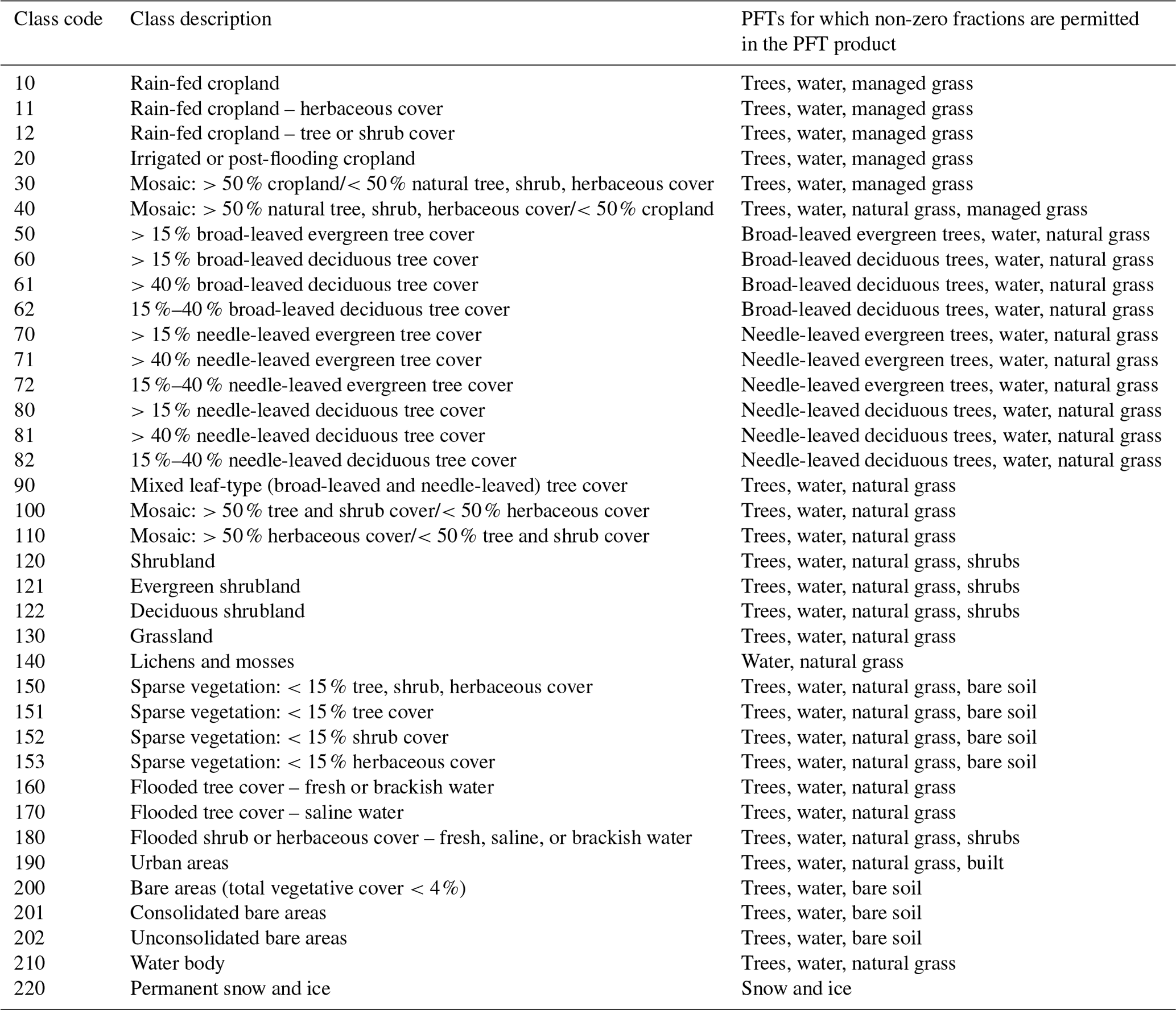
Table 1For each of the 22 global and 15 regional land cover classes of the CCI MRLC map series, listed is the set of contributing PFTs with the possibility of non-zero fractional cover. The regional land cover classes with codes ending in 1, 2, or 3 are thematically richer than the global classes but can be found only at the regional scale depending on training data availability.
2.1 Input datasets
2.1.1 CCI medium-resolution land cover time series (300 m)
The CCI MRLC product (Defourny et al., 2023) delineates 22 primary classes and 15 additional sub-classes of land cover at 10 arcsec (300 m) resolution (Table 1). The maps have global coverage and an annual time step extending from 1992 through 2020, with plans for the continued release of maps for 2021 and future years. The classification system used for the CCI MRLC map series is based on the Land Cover Classification System (LCCS) of the United Nations Food and Agriculture Organization (UN FAO) (Di Gregorio and Jansen, 2005). The LCCS defines fundamental landscape elements called “classifiers” (e.g. trees) forming the class legend when combined in various proportions (e.g. tree cover, broad-leaved, evergreen, closed to open – >15 %). The 15 sub-classes, also called “regional classes”, are defined only in geographic regions where appropriate training data are available and are those with a numeric classification code that has a final digit of 1, 2, or 3 (Table 1). The 22 primary classes and 15 sub-classes are collectively referred to here as simply “classes”. For each year of the time series, each 300 m pixel in the dataset is assigned a single land cover class. The change detection algorithm monitors 13 possible land cover transitions through time. For a pixel to register a change in its assigned land cover class, the algorithm must identify the change for 2 consecutive years in the workflow. A lack of change in a pixel's assigned class does not necessarily indicate an absence of change in the land surface over the time series; rather, it indicates that any change that has occurred in the pixel was limited enough in scale or duration that the assigned class did not change. The full time series and an associated set of quality flags are freely available at https://maps.elie.ucl.ac.be/CCI/viewer/ (last access: 20 March 2023) in GeoTiff and https://cds.climate.copernicus.eu/cdsapp#!/dataset/satellite-land-cover?tab=overview (last access: 20 March 2023) in netCDF. This CCI PFT product is based on v2.0.8 of the CCI MRLC time series, which includes corrections for the known overestimation of cropland relative to grassland in South America (Defourny et al., 2023).
2.1.2 Surface water product (30 m)
The Landsat-based surface water product developed by the Joint Research Centre (Pekel et al., 2016) is used to derive the permanent inland-water fractions at 300 m resolution (calculation details in Sect. 2.2). The surface water occurrence layer (obtained at https://global-surface-water.appspot.com, last access: 20 March 2023) indicates the frequency of water occurrence in each 30 m pixel (80∘ N–60∘ S) over the period March 1984 to December 2019. The frequency occurrence data are reported as integer values of 1 %–100 %, where a value of 100 % occurrence indicates a permanent water surface that existed over the entire analysis period, which encompasses all but the most recent year (2020) of the time series of the MRLC product.
2.1.3 Tree canopy cover product (30 m)
A Landsat-based tree canopy cover product (Hansen et al., 2013) is used to derive the tree cover fractions for 300 m pixels belonging to vegetated classes (except where otherwise noted in Sect. 2.2). The product (obtained at https://glad.umd.edu/Potapov/TCC_2010/, last access: 20 March 2023) is based on the application of a regression tree model to growing-season Landsat 7 ETM+ data (https://glad.umd.edu/dataset/global-2010-tree-cover-30-m, last access: 20 March 2023). The dataset indicates the maximum tree canopy cover percentage (integer values of 1 %–100 %) at 30 m resolution (80∘ N–60∘ S) and is approximately representative of 2010.
2.1.4 Tree canopy height product (30 m)
The global forest canopy height product from Potapov et al. (2021) is used to derive the fractional covers of trees and shrubs in 300 m pixels classified as shrubland. The 30 m product (obtained at https://glad.umd.edu/dataset/gedi/, last access: 20 March 2023) was created by combining the footprint-level lidar forest height measurements (using the 95th percentile relative height metric) for April–October 2019 from the Global Ecosystem Dynamics Investigation with wall-to-wall Landsat optical data to perform spatiotemporal extrapolation. The resulting dataset indicates the canopy height (0–60 m) at 30 m resolution (52∘ N–52∘ S), where canopy heights <3 m were set to 0 m under the assumption that the pixel lacks woody vegetation.
2.1.5 Built-up product (38 m)
The Landsat-based Global Human Settlement Layer (GHSL) dataset produced by the Joint Research Centre (Pesaresi et al., 2013) is used to derive the built-up fraction for 300 m pixels classified as urban land cover by the Global Urban Footprint (GUF) dataset (Esch et al., 2017). The built-up fraction of the PFT dataset is defined as buildings, roads, and artificial structures. The GHSL (alpha version dated November 2014) consists of globally consistent built-up maps for 4 consecutive years (1975, 1992, 2000, and 2014) at 38 m resolution. Built-up areas include both permanent and temporary above-ground buildings.
2.1.6 Zonation products
In addition, three zonation products are used complementarily to consolidate the assignment of the phenology type (deciduous or evergreen) and leaf type (broad-leaved or needle-leaved) to shrubs and, in a very small number of pixels, to trees belonging to a class legend of mixed trees. The Köppen–Geiger climate zone product from Beck et al. (2018) divides the Earth's land surface into 30 distinct climate zones at 0.0083∘ resolution (about 1 km) based on present-day (1980–2016) temperature and precipitation records. Data were obtained at https://figshare.com/articles/dataset/Present_and_future_K_ppen-Geiger_climate_classification_maps_at_1-km_resolution/6396959/2 (last access: 20 March 2023). The landform dataset from Sayre et al. (2014) identifies landforms – surface water, plains, hills, or mountains – at 250 m resolution for 83.6∘ N–56∘ S and is derived from a digital elevation model (USGS GMTED2010: Danielson and Gesch, 2011). The data product was obtained at https://www.usgs.gov/centers/geosciences-and-environmental-change-science-center/science/global-ecosystems-global-data (last access: 20 March 2023). Finally, world regions follow the definitions used in the Integrated Model to Assess the Global Environment 3.0 (IMAGE03) (Stehfest et al., 2014). The IMAGE03 regional classification framework has been harmonized with the CCI MRLC grid by reconstructing the original dataset using the IMAGE-based list of countries per region (available at https://models.pbl.nl/image/index.php/Region_classification_map, last access: 20 March 2023) along with country boundaries from the FAO Global Administrative Unit Layers (available at https://data.apps.fao.org/, last access: 20 March 2023), expanding the list to include Antarctica, Greenland, and additional small islands. The resulting raster dataset divides Earth's surface into 28 regions on the CCI MRLC grid.
2.1.7 CCI medium-resolution water body product
The CCI MRLC water body product (Lamarche et al., 2017) is used to distinguish between inland water and ocean. The dataset (available at http://maps.elie.ucl.ac.be/CCI/viewer/download.php, last access: 20 March 2023) designates all pixels at 150 m resolution as either ocean or non-ocean, the latter of which includes both land and inland water. The dataset is consistent with the water body class (code 210) of the land cover maps of the CCI MRLC. An updated version 4.1 of the product was used here, in which the North American Great Lakes are now considered to be inland water rather than ocean. It is available at http://maps.elie.ucl.ac.be/CCI/viewer/download.php (last access: 20 March 2023).
2.2 PFT dataset development
The overall approach assumes that the definition of the MRLC class is the basis for harmonizing the four existing high-resolution land cover datasets. It proceeds through a systematic sequence of estimating water fraction and tree cover fraction, using tree height to assign life form, and finally deriving phenology. This step-by-step approach is first applied to static pixels before extending it to pixels that undergo changes over time, as identified in the CCI MRLC map series.
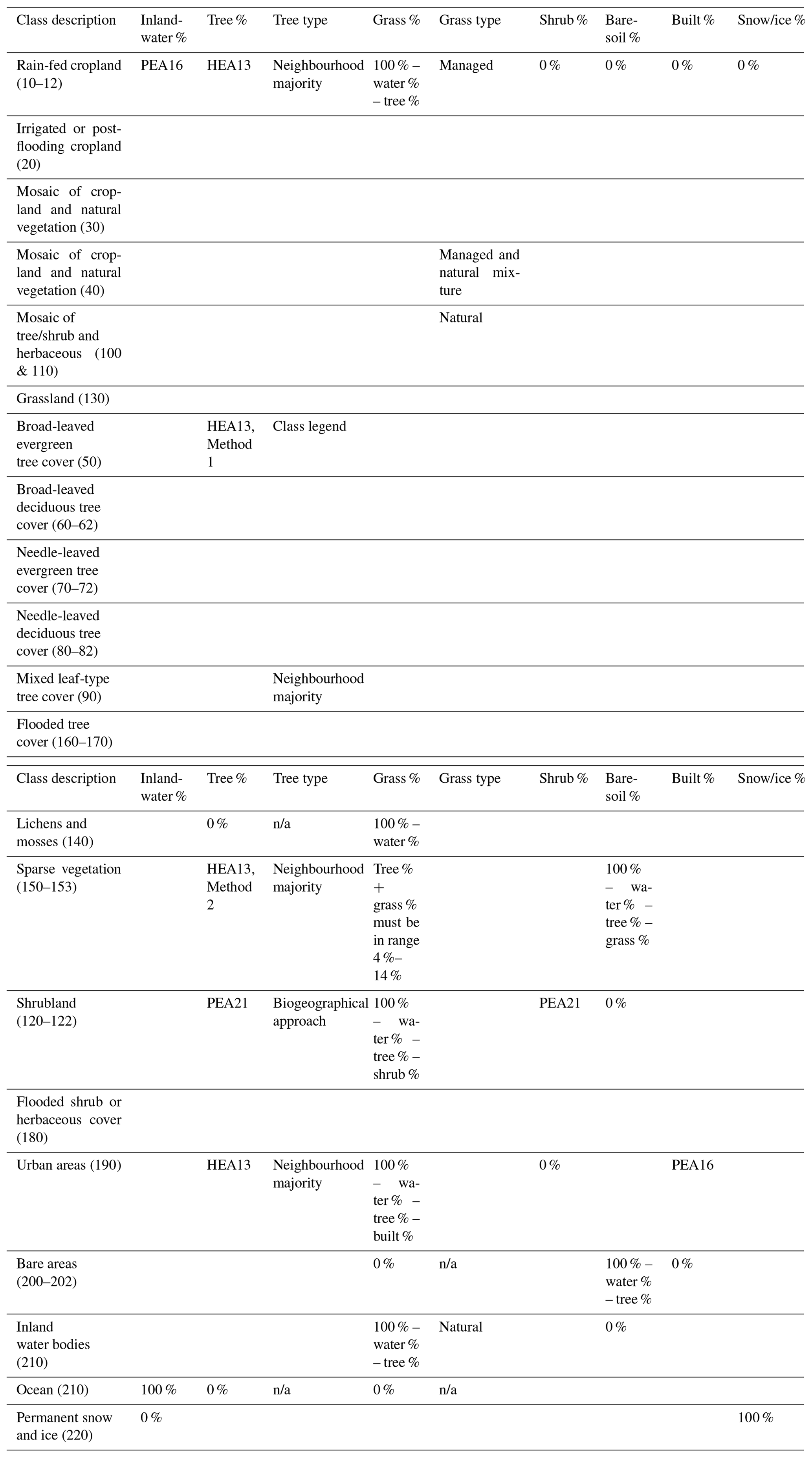
Table 2Summary of the method applied to derive pixel-level functional type composition by land cover class. See Table 1 for more comprehensive class descriptions. PEA16: surface water data product of Pekel et al. (2016). HEA13: tree canopy cover product of Hansen et al. (2013). PEA13: Global Human Settlement Layer from Pesaresi et al. (2013). PEA21: tree canopy height dataset of Potapov et al. (2021). For the calculation of tree percentage, “Method 1” indicates that, in cases of disagreement in tree cover percentage between the ancillary dataset and the class legend, a window of up to is used to estimate the final tree cover percentage based on neighbourhood pixels of the same class, and “Method 3” indicates that an upper limit of 14 % tree cover is applied based on the class definition. See the text for additional details on the processing and use of the ancillary data products, the method used to align the derived PFT percentages with the class legend, the scaling method applied in cases where the sum of PFT percentages from the ancillary data exceeds 100 % in a pixel, and the method used to derive the PFT fractional composition for pixels falling outside of the extents of the ancillary datasets. n/a – not applicable
2.2.1 Static pixels
For static pixels – that is, pixels that have not experienced a class change over the era covered by the CCI MRLC time series (1992–2020) – the derived PFT fractions are treated as temporally invariant for the entire period. Therefore, any intra-pixel change in the fractions of a static pixel is not captured in the PFT map series due to a lack of temporally resolved auxiliary inputs extending over the full time series. Such a change is expected to be so limited in scale and/or duration that it did not prompt a change in class assignment, underscoring the appropriateness of treating the fractional composition of the static pixels as consistent over time.
The same set of auxiliary inputs and the same calculation method are applied to the widest possible set of land cover classes to ensure spatial consistency in the derived PFT fractions. Nonetheless, inherent differences between the classes necessitate the use of different input datasets and methods in some cases. For each class, only a sub-set of the 14 PFTs is permitted non-zero fractions (Table 1). Because the PFT fractional composition is estimated independently for each 300 m pixel of a class, in some cases, an individual pixel of the class can have zero fractional cover even for a PFT that is allowed non-zero cover for that class. For all pixels, the sum of PFT fractions is 100 %. The vegetation thresholds used to define whether pixels are predominantly vegetated or abiotic are based on the definitions of the CCI MRLC classes, which are based on the concepts and definitions of the FAO LCCS (Di Gregorio and Jansen, 2005). Table 2 is a high-level overview of the method used to derive the PFT fractional composition for the static pixels.
The 30 m water frequency occurrence dataset of Pekel et al. (2016) is used to estimate the permanent inland-water fraction of the 300 m pixels for all but the permanent snow-and-ice class, which has no liquid surface water cover. A threshold of 90 % frequency occurrence is applied to assign 30 m pixels as either water (frequency occurrence ≥90 %) or non-water (frequency occurrence <90 %). The resulting binary representation of water/non-water is aggregated to 300 m to estimate the percentage of the 300 m pixel that is a permanent inland-water PFT.
The percentage of the 300 m pixel that is vegetated is calculated as 100 % minus the inland-water percentage; that is, for all vegetation-containing classes except for the sparse-vegetation classes, which have bare-soil PFT cover, all non-inland-water area in the 300 m pixel is entirely vegetated (0 % bare-soil PFT) in the PFT product. Pixels belonging to the shrubland classes (codes 120–122 and 180) can have a mixture of trees, shrubs, and herbaceous cover. For pixels of non-shrubland vegetation-containing classes, the vegetated portion of the pixel is composed of trees and herbaceous cover (i.e. cropland and/or natural grass). The percentage of the 300 m pixel that is tree cover is estimated using the 30 m tree cover dataset for 2010 from Hansen et al. (2013). This Landsat-based dataset provides the percentage of tree canopy cover (integers 1 %–100 %) based on growing-season observations. The tree cover percentage of the vegetated (i.e. non-water) portion of the 300 m pixel is obtained from the median of the tree canopy cover fractions of the non-water 30 m pixels, where the 30 m non-water pixels are identified using the binary water/non-water representation derived using the surface water occurrence dataset. The tree cover percentage of the entire 300 m pixel is calculated as the product of this value (the tree cover fraction of the non-water part of the grid cell) and the non-water fraction of the grid cell. This approach harmonizes the Landsat-based surface water occurrence and tree canopy cover datasets such that the combined tree and water percentages never exceed 100 %.
For the tree cover classes 50–82, the class legend specifies an expected range for the tree cover percentage (Table 1, class description column). For the tree cover classes 90, 160, and 170, a tree cover fraction of >15 % is implicit from the UN LCCS. Based on the spatial and temporal consistency of the map series, deference is made to the class legend for pixels in which the estimated tree cover fraction derived from the auxiliary datasets disagrees with the class legend. This allows the PFT product to retain the advantages of the CCI MRLC map series while improving the translation of the land cover dataset into PFT maps. For tree cover class pixels in which the estimated tree cover fraction derived from the auxiliary datasets disagrees with the class legend, the mean tree cover among all static 300 m pixels of its class is calculated over the 0.25∘ longitude latitude window overlapping the pixel – that is, a window with a width and height of 0.25∘ with the pixel of interest at the centre. The mean is based on the initially calculated tree cover fractions derived from the auxiliary data products (i.e. the tree cover fraction harmonized with the surface water occurrence dataset). The window is expanded to 0.5∘ longitude latitude if no static pixels of the class exist in the smaller window. (Because class 82 has so few pixels globally, class-72 pixels are additionally applied in the window mean calculation for class-82 pixels.) One of five cases is possible.
-
If the mean tree fraction for the window falls within the expected range based on the class legend, then the tree cover fraction of the pixel of interest is assigned as the mean tree fraction for the window.
-
If the mean tree fraction for the window is higher than the upper limit specified by the class legend, then the tree cover fraction of the pixel of interest is assigned as the upper limit from the legend. For classes 62, 72, and 82, the legend upper limit is 40 %. For classes 50, 60, 61, 70, 71, 80, 81, 90, 160, and 170, the legend upper limit is 100 %, and the initial mean tree fraction for the window can never exceed this threshold.
-
If the mean tree fraction for the window is lower than the lower limit specified by the class legend, then the tree cover fraction of the pixel of interest is assigned as the lower limit from the legend. For classes 50, 60, 62, 70, 72, 80, 82, 90, 160, and 170, the legend lower limit is 16 %. For classes 61, 71, and 81, the legend lower limit is 41 %.
-
If a window of does not have any pixels of the class of interest and the tree cover fraction derived from the auxiliary products exceeds the upper limit specified by the class legend, then the tree cover fraction for the pixel is assigned as the upper limit of the class legend.
-
If a window of does not have any pixels of the class of interest and the tree cover fraction derived from the auxiliary products is lower than the lower limit specified by the class legend, then the tree cover fraction for the pixel is assigned as the lower limit of the class legend.
For pixels that belong to a tree cover class and had tree cover percentages assigned using the neighbourhood mean, the resulting sum of the inland-water and tree cover percentages can exceed 100 %. In such cases, the tree cover percentage is calculated as 100 % minus the inland-water percentage. If the resulting tree cover percentage is lower than the legend minimum for that class, then the tree cover percentage is set as the legend minimum and the water percentage is set as the residual area in the pixel (100 % minus tree cover percentage). For all tree-cover-class pixels, the grass cover percentage is calculated as 100 % minus the final tree cover percentage minus the inland-water percentage, and the grass type is assigned as natural grasses. No minimum water percentage is defined for the flooded tree cover classes (codes 160 and 170).
For the biotic classes rain-fed cropland (codes 10, 11, and 12), irrigated or post-flooding cropland (code 20), mosaic of cropland–natural vegetation (codes 30 and 40), mosaic of woody–herbaceous vegetation (codes 100 and 110), and grassland (code 130), the tree cover percentage derived from the auxiliary products is used directly since the legend does not specifically define the expected tree cover; therefore, modification of the PFT fractions based on the class legend is not applied for these classes as it is for some other classes. The percentage of the 300 m pixel that is grass cover is calculated as 100 % minus the sum of the inland-water and tree cover percentages. The grass type – managed (i.e. crops) or natural – is defined by the class legend. For most mixed classes, the assigned grass type reflects the majority type as indicated by the legend. All grass in the pixel is assigned as managed grass for classes 10, 11, 12, 20, and 30. Pixels belonging to mosaic class 40 have a mix of herbaceous crops (up to 49 % of the pixel area) and natural grasses (for excess grass cover beyond 49 % of the pixel area). All grass cover is assigned as natural grass for all other classes.
In some of the classes in this set, an expected percentage cover is given for total woody vegetation (trees and shrubs) or for the shares of cropland and natural vegetation, where the two categories differentiate by management status rather than life form. In the PFT product, shrub cover is estimated only for the shrubland classes due to a lack of appropriate auxiliary inputs to discriminate between trees and shrubs for all classes, so modification of the life form shares in such pixels based on the legend description may introduce additional bias into the PFT product and is therefore avoided. Management status (cropland vs. natural) is assigned in the PFT product only for grasses and is based on the class descriptions, so an independent assessment of the shares by management status is not possible.
Pixels belonging to the sparse-vegetation classes (codes 150, 151, 152, and 153) can have non-zero fractions of bare soil, trees, natural grass, and inland water. The class definition requires a vegetation fraction of 4 %–14 %. Since shrub cover is not estimated for the sparse-vegetation classes, the vegetation component is composed of trees and natural grasses; therefore, the total vegetation fraction is enforced for sparse-vegetation pixels, but the resulting life form may differ from that indicated by the legend for the sub-classes with codes 151–153. If the tree cover derived from the auxiliary inputs is ≥15 %, then the tree PFT is reduced to 14 % in deference to the legend of the CCI MRLC map series, the natural-grass PFT is assigned as 0 % since tree cover accounts for the maximum total vegetation fraction (trees + grass), and the bare-soil PFT percentage is calculated as 100 % minus the inland-water percentage minus 14 % tree PFT. If the tree cover derived from the auxiliary inputs is <15 %, then this input tree percentage value is assigned as the final tree PFT percentage in the pixel and additional legend-consistency steps are applied to assign the grass and bare fractions. (1) If the non-water area of the pixel is 4 %–14 %, then the natural-grass PFT accounts for the residual portion of the pixel (14 % minus tree PFT percentage minus inland-water percentage). (2) If the non-water percentage of the pixel is <4 %, then the natural-grass PFT percentage is calculated as 4 % minus the tree PFT percentage (since the lower bound on total vegetation is 4 %) and the water PFT percentage is scaled down to 96 %. (3) If the non-water percentage of the grid cell exceeds 14 %, then the natural-grass percentage is calculated as 14 % minus the tree PFT percentage (that is, the upper bound of 14 % is assumed for total vegetation cover) and the residual pixel area is assigned as bare-soil PFT (100 % minus water PFT percentage minus 14 % vegetation cover).
A mixture of the tree and shrub woody vegetation types is assigned to pixels of the shrubland classes (codes 120, 121, 122, and 180). The 30 m resolution tree canopy height dataset from Potapov et al. (2021) is applied to discriminate between shrubs and trees in pixels that are covered by this data product (52∘ N–52∘ S). Potapov et al. (2021) re-assign pixel values of ≤2 to 0 m height. Here, the 30 m resolution pixels are assigned to three broad height classes: 0, 3–5, and >5 m. Mean re-sampling to the 300 m resolution of the land cover dataset results in pixel values that indicate the percentage cover of the three height classes. The percentage cover of the 3–5 m height class is taken to be the percentage shrub cover in the 300 m pixel, and the percentage cover of the >5 m height class is taken to be the percentage tree cover in the 300 m pixel, recognizing that there may be some bias introduced by 30 m pixels in the input dataset that contain both shrubs and trees. In deference to the class legend, 300 m pixels with shrub cover <16 % are assigned as having 16 % shrub cover and those with tree cover >15 % are assigned as having 16 % tree cover. For shrubland pixels that occur outside of the extent of the Potapov et al. (2021) data product (52∘ N–52∘ S), the tree cover percentage is assigned according to the tree cover input derived from Hansen et al. (2013) and the shrub cover percentage is assigned following the most recent version of the global cross-walking table (CWT) (60 % shrub cover for classes 120–122 and 40 % shrub cover for class 180). For all shrubland pixels, in cases where the sum of water, tree, and shrub cover exceeds 100 %, the three PFTs are scaled down proportionally so that the sum is 100 % while retaining the legend expectations for the tree and shrub cover. Natural-grass cover is assigned as the residual area of the pixel in cases where the sum of water, tree, and shrub cover is <100 %. No minimum water percentage is defined for the flooded-shrubland class (code 180).
Pixels classified as urban (code 190) can have non-zero fractions of inland-water, tree, natural-grass, and urban impervious (built-up) PFTs. In the land cover classification, pixels are assigned as an urban class when a minimum threshold of 50 % built was exceeded based on the GUF dataset (Esch et al., 2017). In the PFT product, the tree and surface water fractions are derived using the same protocol as the one applied to the vegetated classes. The urban impervious fraction is derived from the GHSL dataset (Pesaresi et al., 2013) by aggregating the built-up pixels from the four epochs into a binary built-up/non-built-up distribution at 38 m. Re-sampling to 300 m provides the percentage of the 300 m pixel that is built PFT, introducing local variability which at the global scale ranges from 0 % to 100 % built. Only pixels classed as urban by GUF are assigned a non-zero urban impervious fraction in the PFT dataset. Non-urban pixels (i.e. those with less than 50 % urban land cover according to GUF) are not refined with GHSL data or assigned a built-up percentage. The GHSL appears to capture urban impervious areas more consistently, whereas GUF misses road fractions in the built fractions. This is most notable in rural areas and a few selected locations in city centres. If the sum of the urban impervious, tree, and water fractions exceeds 100 %, then the urban impervious percentage is retained and the water and tree percentages are scaled down proportionally to a total sum of 100 %; otherwise, the residual of the urban impervious, tree, and water percentages is assigned as the natural-grass percentage.
Water-body-class (code 210) pixels that are ocean are assigned as a 100 % water PFT, while those that are inland can additionally have a non-zero cover of tree and natural-grass PFTs. The designation of ocean vs. inland at 300 m is determined using the 150 m water body product. The ocean designation is applied to water-body-class pixels in which all four of the overlapping 150 m pixels of the water body product are classified as ocean; all other water-body-class pixels are designated as inland water. The water and tree PFT fractions for inland water-body-class pixels are assigned using the same 300 m harmonized surface water and tree cover auxiliary inputs that are used for the other classes; however, a minimum of 86 % water PFT is enforced following the legend definition for this class. If the sum of the tree fraction and the adjusted water PFT fraction exceeds 100 %, then the tree percentage is scaled down as 100 % minus the adjusted water PFT percentage. Any residual area is assigned as the natural-grass PFT.
The bare-area classes (codes 200, 201, and 202) can have up to 3 % vegetation cover (by definition of the abiotic class in the FAO LCCS; Di Gregorio and Jansen, 2005), so bare-area pixels can have non-zero fractions of bare-soil, tree, and water PFTs. The auxiliary products define the tree and inland-water fractions, but tree cover exceeding 3 % is scaled down to the class maximum of 3 %. Bare-soil PFT percentage is calculated as 100 % minus the inland-water percentage minus the tree percentage. Pixels of the moss and lichen class (code 140) can have non-zero fractions of surface water and natural grasses, the latter of which are estimated as 100 % minus the inland-water percentage.
The permanent snow-and-ice class (code 220) is assigned as a 100 % snow-and-ice PFT. All other classes are assigned as a 0 % snow-and-ice PFT. Nearly all pixels classified as the permanent snow-and-ice class in the CCI MRLC time series are static pixels; that is, such pixels are snow-and-ice cover for every year of the land cover map series. This is due to a lack of temporally resolved input data available at the global scale to track the evolution of this surface type. Therefore, neither the CCI MRLC classification nor the associated PFT product should be used to track changes in glaciers over time.
For all pixels – of any class – that have a non-zero tree fraction, the total tree fraction is assigned as a single tree type (broad-leaved or needle-leaved leaf type, deciduous or evergreen phenology). For the tree cover classes coded 50–82, the specific tree type follows the class legend. For example, class 50 is defined as “Tree cover – broad-leaved evergreen >15 %”, so the tree component of this class is assigned as the broad-leaved evergreen tree type. Tree cover is assigned as broad-leaved deciduous in pixels of classes 60–62, needle-leaved evergreen in pixels of classes 70–72, and needle-leaved deciduous in pixels of classes 80–82. For pixels of the tree cover classes coded 90, 160, and 170 and all other vegetation-containing classes except the shrubland classes, the specific tree type is assigned by pixel based on the majority tree type in the surrounding neighbourhood window, where the majority calculation is performed on static pixels of the tree cover classes with legend-defined tree types (classes 50–82). If the window does not contain any static pixels of the well-defined tree types, then the window is incrementally expanded by 0.25∘ in each direction (longitude and latitude) to a maximum window size of until such a pixel is contained within the search window. The same tree type is assigned to all pixels in a class for tree cover classes 50–82, while the assigned tree type can vary between pixels within a class for the other classes. The vast majority (75 %) of pixels with a non-zero tree fraction were assigned a tree type directly using the class legend; an additional 24 % had tree type assigned using a surrounding window of , <1 % using a larger window up to a size of , and <0.1 % using an even larger window up to a size of .
For a very small number of pixels, static pixels of the type-defined tree cover classes are absent from the surrounding window, so a climatological approach is instead used to assign the tree type to such pixels. This approach uses three auxiliary inputs: (1) the present-day Köppen–Geiger climate zone map from Beck et al. (2018), downscaled from 1 km resolution to the 300 m CCI MRLC grid using mode resampling, (2) the map of world regions derived for use with the IMAGE03 model, expanded to include Greenland, Antarctica, and additional small islands, and (3) the landform map from Sayre et al. (2014), resampled from 250 m resolution to the 300 m CCI MRLC grid using mode resampling. A nearest-neighbour analysis is used to gap-fill missing data at 300 m resolution for each of the three auxiliary inputs. Pixels requiring data are those with <100 % water PFT cover in the PFT product. Pixels that are designated as surface water in the landform dataset and have <100 % water PFT cover in the PFT product are additionally filled with one of the terrestrial landforms (plains, hills, and mountains). Missing data generally occur along coastlines due to mismatches in the land–sea masks of the auxiliary datasets and the CCI MRLC data. The gap-filled datasets are combined to create a dataset of 1531 unique combinations of landform, region, and climate zone. For each of the unique combinations, the areal cover of each of the tree cover classes with well-defined tree types (codes 50–82) is calculated using static pixels of those classes, and the majority tree type by area is identified for each unique combination. There are very few static pixels of the type-defined tree cover classes in the Middle East and Sahara regions, so the dominant tree type in these regions is set as broad-leaved deciduous. For pixels in which the tree type – broad-leaved or needle-leaved, deciduous, or evergreen – cannot be assigned based on the neighbourhood window, the majority tree type of the pixel's unique zone is assigned. This method is also applied to assign the types of both shrubs and trees in all shrubland-class pixels. Thus, there may be inconsistencies between the shrub type indicated by the class legend and that assigned using this biogeographical approach.
Most of the auxiliary inputs are based on Landsat images and therefore have an extent of 80∘ N–60∘ S. The main processing algorithm for the PFT product, explained above for the static pixels, therefore operates on this extent. Less than 0.5 % of the area outside of this extent is composed of pixels belonging to a class other than water bodies (code 210) or permanent snow and ice (code 220). The largest contributors to this small area are the sparse-vegetation classes, followed by the bare-area classes, with negligible contributions from the shrubland (including flooded shrubland), grassland, and lichen and moss classes. To extend the PFT product to global extent, the following assumptions are applied to the pixels north of 80∘ N and south of 60∘ S: (1) 100 % snow-and-ice PFT assigned to pixels of the permanent snow-and-ice class; (2) 100 % water PFT assigned to pixels of the water body class; (3) 100 % bare-soil PFT assigned to pixels of the bare-area classes; (4) 100 % natural-grass PFT assigned to pixels of the grassland and lichen and moss classes; (5) 96 % bare-soil PFT and 4 % natural-grass PFT (to meet the legend minimum of vegetation cover) assigned to pixels of the sparse-vegetation classes; (6) 84 % natural-grass PFT and 16 % needle-leaved deciduous shrub PFT (matching the legend minimum shrub cover) assigned to pixels of the shrubland classes. For the shrubland classes, the shrub type of needle-leaved deciduous is assigned because the shrubland-class pixels needing assignment (northern–central Russia) occur nearest pixels of needle-leaved deciduous shrubs that had their shrub type assigned using the standard method.
2.2.2 Pixels experiencing land cover change
Dynamic pixels – that is, pixels that have experienced at least one land cover class change over the 1992–2020 era – correspond to 5.88 % of the ice-free land surface (Defourny et al., 2023). For such pixels, the derived PFT fractions are derived for each of the classes assigned to that pixel over the era. For example, if a pixel changed from forest to cropland, PFT fractions associated with the forest class are estimated and PFT fractions associated with the cropland class are also estimated for the pixel. The method used to assign the PFT fractions depends on the time stamp of the class in relation to the time stamp (2010) of the auxiliary dataset (Hansen et al., 2013) from which the tree cover fractions are derived. The PFT fraction of a pixel in 2010 was derived using the following class-specific methods described in Sect. 2.2.1. Any change in class occurring before or after 2010 leads to derivation of new PFT fractions as the mean PFT fractions of all 300 m pixels of the same class of pixels within the overlapping window centred on the pixel of interest. The input pixels over which the mean is calculated are the 300 m pixels that did not experience land cover class change over the 1992–2020 era. If no pixels of the relevant class are within the window, then the window is incrementally expanded by 0.25∘ in both the latitudinal and longitudinal directions until at least one pixel of the relevant class is contained in the window. A pixel can experience up to seven land cover changes in the 1992–2020 era (Defourny et al., 2023), which leads to derivation of new PFT fractions for each new land cover class encountered.
2.3 Modelling assessment
The impact of the updated PFT distribution on land surface fluxes is evaluated using global simulations of two land surface models: ORCHIDEE (Krinner et al., 2005, and later revisions) and JULES (Best et al., 2011; Clark et al., 2011). The simulations with ORCHIDEE focus on evaluating the impact of the updated PFT distributions on a selected set of climate-relevant variables. The ORCHIDEE model applies the Climatic Research Unit (CRU)–Japanese reanalysis (JRA55) v2.0 6 h atmospheric driving data for 1901–2018 (Harris et al., 2014; Kobayashi et al., 2015; UEA CRU and Harris, 2019) and the CCI PFT distribution maps for 2010. Two PFT distributions are applied: (1) the new PFT map (PFTlocal) described above and (2) the PFT distribution based on the application of the global standard CWT to the CCI MRLC product for 2010 (PFTglobal) (Table C1) (Hartley et al., 2017; Lurton et al., 2020). The 2010 PFT map is used (recycled) for each year of the simulation. ORCHIDEE is run at a horizontal resolution of 0.5∘ latitude longitude over the period 1900–2018, and all simulated data before 1980 are discarded as spin-up, with analysis based on the years 1980–2018. The impact of the updated distribution relative to that based on the global CWT is compared with ORCHIDEE for an ensemble of climate-related variables, including albedo, surface fluxes (latent and sensible heat and their ratio), gross primary productivity, surface temperature, tree fraction, leaf area index (LAI), and above-ground biomass (Sect. 4).
In a separate assessment of the implications of the updated PFT distributions for model evaluation, JULES simulations of PFT distributions, created for the Inter-Sectoral Impacts Model Inter-comparison Project (ISIMIP; Frieler et al., 2017), were used. This was done to compare evaluation results using both the CWT-derived PFT distributions (PFTglobal) and the updated PFT distributions (PFTlocal). The 2010 PFT distributions are used to evaluate the JULES dynamic vegetation results. JULES was driven by the ISIMIP2b protocol described in Frieler et al. (2017) and applied to JULES as described in Mathison et al. (2022). Section 4.2 describes the dynamic global vegetation model (DGVM) results for 2010 from the JULES offline simulations driven by HADGEM2-ES climate for the period 1850 to 2100.
3.1 General description
The CCI PFT dataset (hereafter called PFTlocal) provides the percentage cover as discrete values of 0 %–100 % of 14 PFTs at 10 arcsec resolution (300 m at the Equator; 64 800 pixels in the latitudinal dimension ×129 600 pixels in the longitudinal dimension). The global continuous field maps are produced at an annual resolution covering the years 1992–2020. The PFT distributions are consistent with the CCI MRLC data product and eliminate the need to use a CWT to translate land cover classes into PFTs. The 14 PFTs encompass the following. (1) Permanent inland-water bodies; (2) permanent snow-and-ice cover; (3) bare soil; (4) built-up areas, which include artificial impervious area such as buildings and, frequently but not exhaustively, other paved surfaces such as roads; (5) managed grasses (i.e. herbaceous crops); (6) natural grasses (i.e. non-cultivated herbaceous vegetation); (7) broad-leaved deciduous shrubs; (8) broad-leaved evergreen shrubs; (9) needle-leaved deciduous shrubs; (10) needle-leaved evergreen shrubs; (11) broad-leaved deciduous trees; (12) broad-leaved evergreen trees; (13) needle-leaved deciduous trees; (14) needle-leaved evergreen trees (Fig. 1). Following the auxiliary inputs, trees are woody vegetation with a height of >5 m, while shrubs are woody vegetation with a height of 3–5 m inclusive. An updated water body product (version 4.1) at 150 m resolution, used here to delineate between inland water and ocean, likewise replaces the older version and can be downloaded from the same data repository as the PFT maps.
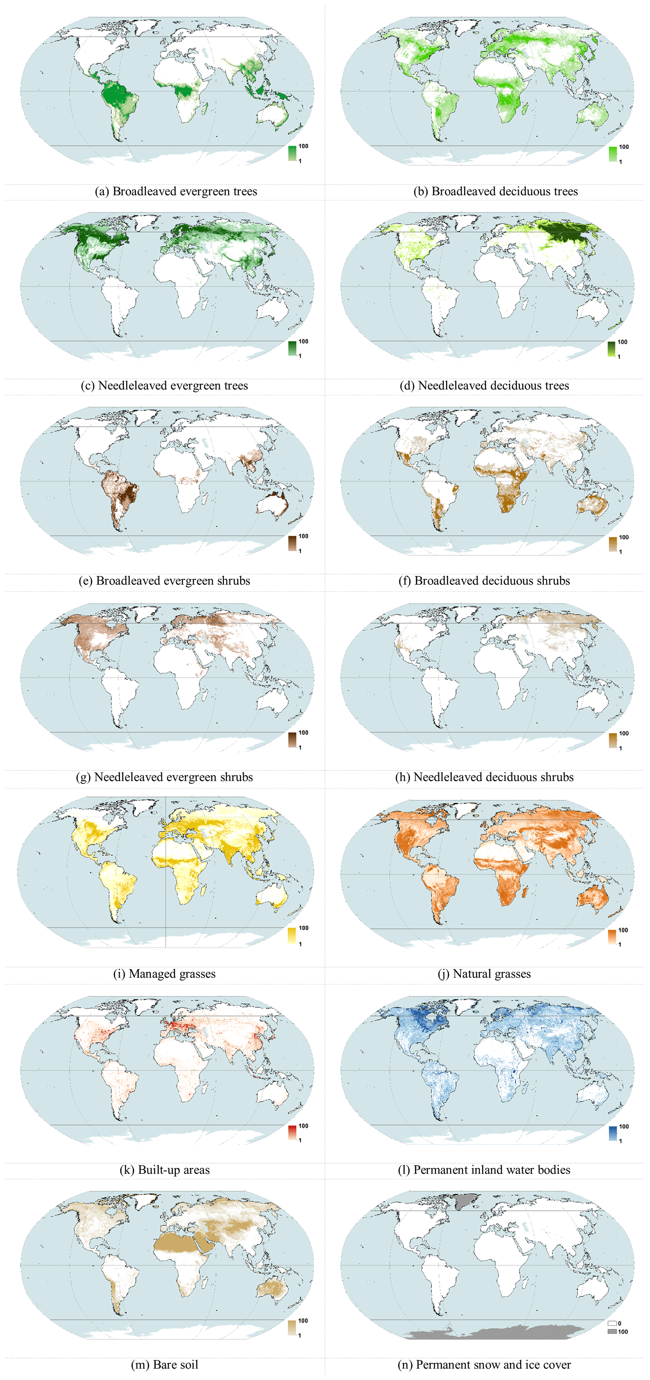
Figure 1Percentage cover in 2010 for the 14 PFTs included in the PFTlocal data product at a spatial resolution of . (a) Broad-leaved evergreen trees, (b) broad-leaved deciduous trees, (c) needle-leaved evergreen trees, (d) needle-leaved deciduous trees, (e) broad-leaved evergreen shrubs, (f) broad-leaved deciduous shrubs, (g) needle-leaved evergreen shrubs, (h) needle-leaved deciduous shrubs, (i) managed grasses, (j) natural grasses, (k) built-up areas, (l) permanent inland-water bodies, (m) bare soil, and (n) permanent snow-and-ice cover.
The PFTlocal dataset indicates that herbaceous vegetation covers 44.8 % of the Earth's land surface, with around one-third of that area devoted to herbaceous crops. Tree cover accounts for 21.3 % of the land surface, which is much larger than that of shrubs (3.2 %). The abiotic surface types cumulatively cover 30.8 % of the land surface: 18.4 % bare soil, 10.0 % snow and ice, 2.1 % inland water, and 0.3 % built.
The CCI PFT dataset is provided as a companion product to the ESA CCI LC map series products with similar specifications with a global extent, a pixel size of 300 m, and a plate carrée projection. However, climate models may need products associated with a coarser spatial resolution, over specific areas (e.g. for regional climate models), and/or in another projection. To tackle the variety of requirements, a user tool has been developed that allows users to adjust the products in a way which is suitable to their models. A minimum list of possibilities in terms of spatial resolution and projection has been established, and the conversion of CCI-Land Cover classes to other user-defined classes is also foreseen. The CCI PFT product and the user tool are freely available at http://maps.elie.ucl.ac.be/CCI/viewer/ (last access: 20 March 2023) and https://climate.esa.int/en/projects/land-cover/data/ (last access: 20 March 2023).
Table 3Global areal cover (1000 km2) of each PFT by land cover class for 2010 in the PFTlocal product.

* For the water body class (code 210), the water PFT area includes 2 877 500 km2 of inland water. For all other classes, all water PFT area is inland water.
3.2 PFT-layer description considering the CCI MRLC categories and the PFTglobal dataset
Table 3 shows the global areal coverage of each PFT by class for 2010 for the PFTlocal product, and Table A1 shows the equivalent data corresponding to the application of the most recent version of the CCI MRLC global CWT (Lurton et al., 2020; Table A2) to the v2.0.8 CCI MRLC map for 2010 (hereafter called PFTglobal). Figure A2 complements Table A1 by illustrating the differences between the PFTlocal and PFTglobal products globally at a spatial resolution of . For each class of PFTglobal, the global CWT specifies the fractional composition of contributing PFTs. In this approach, each pixel of a class is assigned the same fractional PFT composition regardless of its location on Earth. Table 4 indicates the percentage PFT composition by class for 2010 for PFTlocal, calculated as an area-weighted mean taken over all pixels of the class globally. Figure A3 provides a spatialized summary of the largest differences between the PFTlocal and PFTglobal products. (a) PFTs with the largest increase, (b) corresponding fraction gained, (c) PFT loss, and (d) corresponding fractions lost are illustrated globally with pixels.
Table 4Percentage PFT composition by class for 2010 calculated as an area-weighted mean over all pixels of the class globally.
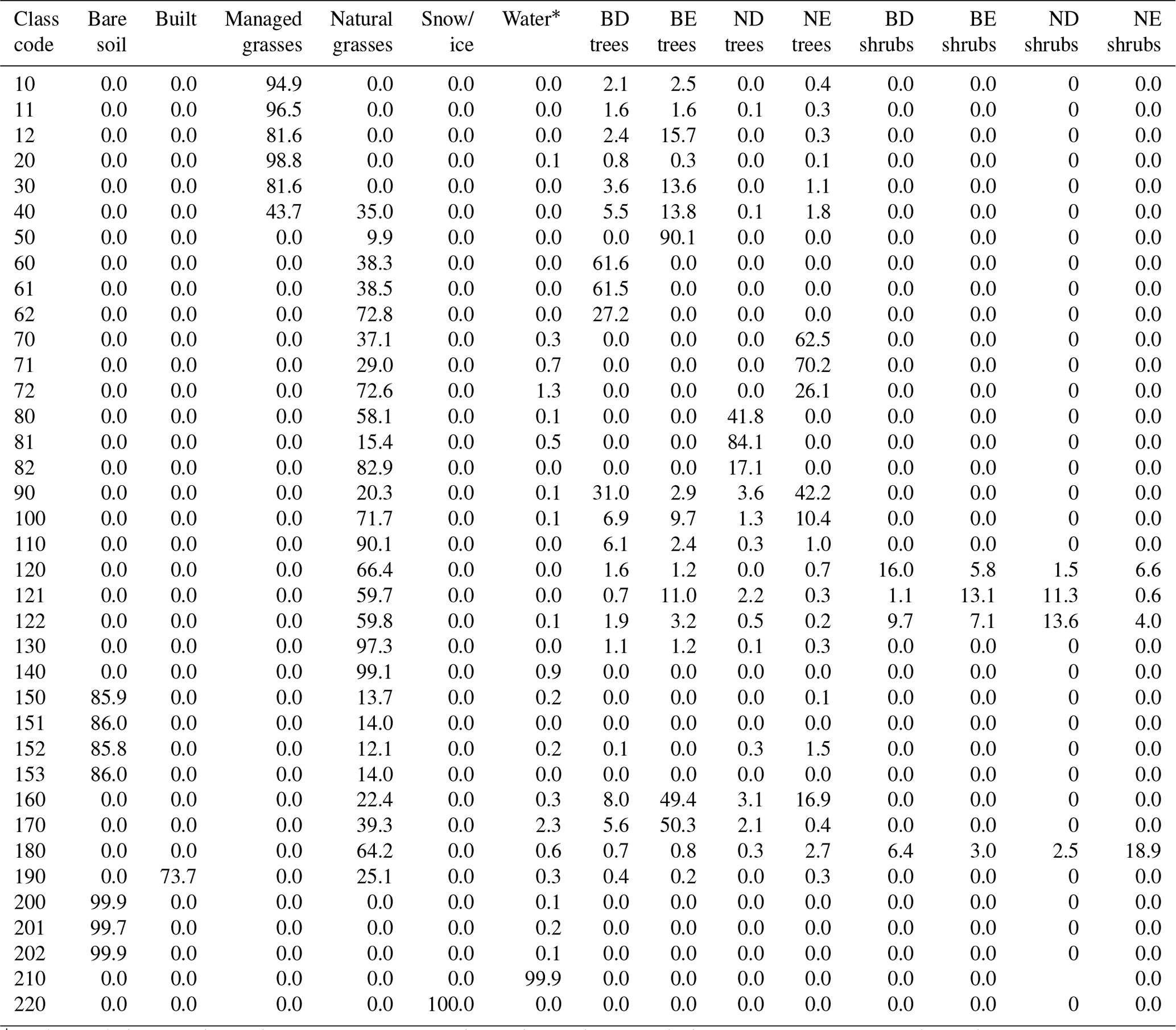
* For the water body class (code 210), the water PFT percentage includes inland water. The area-weighted mean percentage composition of the inland-water PFT in water-body-class pixels is 0.8 %. For all other classes, all water is inland water.
3.2.1 Tree cover
The PFTlocal product indicates a global areal tree cover of 31.4 × 10⁶ km2 (Fig. 1): 45.2 % broad-leaved evergreen; 24.3 % needle-leaved evergreen; 23.0 % broad-leaved deciduous; 7.5 % needle-leaved deciduous. The PFTlocal product indicates a global areal tree cover that is 4.6 % higher than in the PFTglobal distribution. Globally, tree coverage is higher in the PFTlocal product relative to the PFTglobal distribution for all tree types except needle-leaved deciduous trees. Compared to the global CWT, in which every pixel belonging to a given class is assigned the same PFT fractions, the updated method for estimating PFT fractions locally results in greater variability of tree fractions among 300 m pixels within a single class. For example, the global CWT suggests that all class-10 (rain-fed cropland) pixels are 0 % tree cover, but the PFTlocal product based on auxiliary inputs suggests a much wider range of tree cover at the pixel level, ranging from 0 % to 100 % tree cover at the 300 m pixel level. The distribution for Africa is shown in Fig. A1, where tree crops in the Sahel are readily apparent. Globally, class-10 pixels have 5.1 % tree cover on average (Table 4). On average, class-12 pixels (rain-fed cropland – tree or shrub cover) have 18.4 % tree cover. The auxiliary dataset used to derive tree cover for most classes in the PFTlocal product is based on Landsat 7 images (Hansen et al., 2013); the artifacts associated with the failure of the Landsat 7 Scan Line Corrector (Andrefouet et al., 2003) are visible in the 300 m PFTlocal dataset in some regions, particularly in western–central Africa. Because the PFT product is harmonized with the CCI MRLC class product, potential classification errors can impact the PFT product. For example, recent high-resolution mapping in the circumpolar Arctic (Bartsch et al., 2019) suggests that the CCI MRLC classification may overestimate needle-leaved evergreen tree cover in this region, resulting in a possible overestimate of the tree PFT percentage in such pixels. Future improvements to the land cover classification will likewise flow through to the PFT product.
3.2.2 Shrub cover
The PFTlocal product indicates 4.7 × 10⁶ km2 of global shrub cover. The largest contributors to total shrub cover are broad-leaved deciduous (44.6 %) and needle-leaved evergreen (25.2 %) shrubs. Shrub cover is 74 % lower in the PFTlocal product than in the PFTglobal dataset. Some of this difference arises because the PFTlocal product estimates a lower shrub PFT in shrubland-class pixels (codes 120–122 and 180) compared to the PFTglobal dataset, which estimates 8.8 × 10⁶ km2 of the shrub PFT in shrubland classes. The area-weighted mean percentage composition of shrubs in shrubland-class pixels is 30.0 % for class 120 in the PFTlocal product, 26.1 % for class 121, 34.4 % for class 122, and 30.7 % for class 180. The CWT suggests 60 % shrub cover for classes 120–122 and 40 % for class 180. The CWT estimates 0 km2 of tree PFT cumulatively in these classes compared to 630 000 km2 in the PFT product. The uncertainty associated with the height estimation in the global canopy height product of Potapov et al. (2021) may contribute to the confusion of shrubs and trees in some cases. Nonetheless, the evidence-based PFTlocal product indicates a significantly lower estimate for global woody vegetation cover in pixels of the shrubland classes compared to the PFTglobal dataset, which was largely based on expert knowledge.
In addition to the differences in the shrubland-class pixels, a large part of the difference in total shrub cover between the PFTlocal product and the PFTglobal dataset can be ascribed to the fact that the PFTlocal product estimates shrub PFTs only in pixels belonging to the shrubland classes (codes 120–122 and 180) due to a lack of appropriate datasets to apply to the other classes. The CWT estimates 9.5 × 10⁶ km2 of shrub cover in non-shrubland PFTs, and some of this shrub cover may indeed be missing from the PFTlocal product. However, because the PFTlocal product, which is based on quantitative estimation using auxiliary inputs, and the CWT, which is largely based on expert input, differed so strongly in the estimates of shrub PFTs in the shrubland-class pixels, some of the differences in the non-shrubland-class pixels may likewise be due to bias in the CWT.
3.2.3 Natural and managed grasses
Global grass PFT cover in the PFTlocal product is 65.7 × 10⁶ km2, two-thirds of which is natural grass. Total grass cover is 29.6 % higher in the PFTlocal product than in the PFTglobal map (38.3 % higher for natural grass and 14.7 % higher for managed grass). In the PFTlocal product algorithm, for the vegetated classes except for sparse vegetation, the entire non-water fraction of the 300 m pixel is assigned as vegetation; typically, water, trees, and other PFTs are estimated based on auxiliary inputs and the CCI MRLC class legend, and then the residual area is assigned as grass cover. Thus, grass vegetation may be assigned in some cases that might otherwise be a temporary bare area.
3.2.4 Water
In the PFTlocal product, the per-pixel fraction of surface water PFT is estimated for pixels of all classes except the permanent snow-and-ice class (Table 1). The PFTlocal product indicates around 142 000 km2 of water cover globally among pixels of all classes except the water body class (code 210). Only two classes – a sparse-vegetation sub-class (code 151) and a needle-leaved deciduous tree cover sub-class (code 82) – have no pixels with inland-water cover (Table 3), but both classes have extremely limited total areal coverage, each accounting for only a few square kilometres of area globally. Classes with significant water coverage include the needle-leaved evergreen tree cover classes 70 and 71 (40 000 km2 combined), sparse-vegetation class 150 (20 000 km2), lichen and moss class 140 (14 000 km2), flooded-shrub/herbaceous-cover class 180 (12 000 km2), and bare-area class 200 (12 000 km2). Coverage of the water PFT in pixels of the non-water-body classes is especially prevalent in the boreal region. Classes with the highest fractional composition of inland water – calculated as the area-weighted mean among all pixels of the class globally (Table 4) – include the flooded tree cover class 170 (2.3 %), the needle-leaved evergreen tree cover class 72 (1.3 %), and the lichen and moss class 140 (0.9 %).
The PFTlocal product indicates 3 % (91 000 km2) lower inland-water fractional cover than the PFTglobal product distribution. While the non-water-body classes have a total inland-water PFT cover of 142 000 km2 in the PFTlocal product (compared to 0 km2 from PFTglobal), the PFTlocal product indicates a lower inland-water PFT area in the water body class than the CWT (difference of 233 000 km2). The difference in the water body class occurs because the PFTlocal product allows up to 14 % vegetation cover in this class, whereas the CWT assumes a 100 % water PFT. PFTs with significant global coverage in water-body-class pixels in the PFTlocal product include natural grasses (183 000 km2) and needle-leaved evergreen trees (31 000 km2), with smaller contributions from the other tree types.
3.2.5 Bare
In the PFTlocal product, the bare-soil PFT occurs in the bare-area classes (codes 200–202) and the sparse-vegetation classes (codes 150–153), accounting for 19.4 and 7.6 × 10⁶ km2 of bare-soil area, respectively, at the global scale (Table 3). The global area-weighted mean bare-soil percentages are 85.9 % in sparse-vegetation-class pixels and 99.9 % in bare-area-class pixels, which are nearly identical to the compositions suggested by the global CWT (85 % for sparse-vegetation classes and 100 % for bare-area classes). Cumulatively for these classes, the PFTlocal product suggests only 0.2 % lower bare-soil PFT coverage at the global scale relative to the assumed distribution in the PFTglobal dataset (difference of 65 000 km2). In the PFTlocal product, the bare-area classes contain, in addition to the bare-soil PFT, an inland-water PFT (13 000 km2) and tree cover (1000 km2).
The PFTlocal product does not include the bare-soil PFT in the shrubland classes, while the PFTglobal dataset assumes 20 % bare soil for non-flooded-shrubland classes 120–122. Because the non-flooded shrubland-class pixels have such a large extent globally (13.3 × 10⁶ km2), the PFTglobal dataset suggests 2.7 × 10⁶ km2 of additional bare soil in such pixels relative to the PFT product. Differences in the distribution of bare area between the PFTlocal product and the PFTglobal product are especially pronounced in the US inter-mountain west, parts of southern and eastern Africa, the northern coast of Australia, and the highlands of Argentina and Brazil, as these are regions with significant shrubland-class cover. In the PFTlocal product, all residual area in the shrubland-class pixels that is not assigned as surface water or woody vegetation (trees and/or shrubs) based on the auxiliary input data is assigned as natural-grass cover rather than bare soil.
In the PFT local product, the bare-soil PFT represents areas that are not expected to support vegetation regardless of environmental conditions. For shrubland-class pixels, we assume that vegetation growth can be supported given the appropriate environmental conditions; therefore, the residual pixel area (after accounting for inland water, tree, and shrub cover) is assigned as the natural-grass PFT. Since the PFTlocal product is built mainly for application to land surface models, the actual presence of grass vegetation vs. bare soil for such pixels (of the shrubland class, but also of the other vegetated classes) will be determined by the model given simulated or prescribed local climate conditions. Users should consider the definition of the bare-soil PFT to determine the suitability of the data product for their use case.
3.2.6 Built fraction
Both the PFTlocal product and the PFTglobal product assign a built PFT only to pixels of the urban class (code 190). The presence of a built PFT is not universal in land surface or Earth system models; for example, the current version of the ORCHIDEE land surface model considers built areas to be 80 % bare soil and 20 % grasslands. The cross-walking of land cover classes to PFTs for the urban class strongly depends on the framework used to calculate surface fluxes in the urban environment, and therefore inter-model variation in the global CWT may be stronger for the urban class than for the vegetated classes. The global CWT used for this analysis assigns 100 % of the urban class as the built PFT. For comparison, the JULES land surface model assigns urban-class pixels as 75 % built and 25 % bare soil.
The PFTlocal product suggests 477 000 km2 of built area globally (Table 3), which corresponds to an area-weighted mean composition of 73.7 % built PFT in urban-class pixels (Table 4). The auxiliary inputs suggest that about 1.6 % of urban-class pixels have 0 % built-PFT coverage. This suggests a mismatch between the land cover classification and the auxiliary inputs for a small number of pixels, which could be related to a mismatch in the time stamp of the auxiliary inputs (2014) relative to the land cover dataset. Considering all urban-class pixels, 6.2 % have a built PFT of 0 %–25 %, 7.8 % have a built PFT of 26 %–50 %, 31.9 % have a built PFT of 51 %–75 %, and 54.1 % have a built PFT of 76 %–100 %. As area-weighted means, the non-built portion of urban-class pixels is 25.1 % natural-grass cover, 0.3 % inland water, and 0.9 % tree cover. The increased spatial heterogeneity in urban-class pixels due to the PFTlocal product is readily apparent in Fig. 2, which shows the PFT distribution for Amsterdam, the Netherlands. The more realistic characterization of the urban environment in the PFTlocal product that gives more variability of built-PFT coverage within a city should allow a more faithful representation of urban surface fluxes in land surface models.
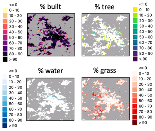
Figure 2Percentage cover in 2010 for the built, total tree, grass, and inland-water PFTs in Amsterdam, the Netherlands, in the PFTlocal product.
3.2.7 Permanent snow and ice
The permanent snow and ice in PFTlocal account for 14.7 × 10⁶ km2 in area globally, largely in Greenland and Antarctica, but also in the Arctic and mountainous regions of Asia. The PFTlocal product and the PFTglobal dataset indicate identical coverage for this PFT since both datasets assign a 100 % snow-and-ice PFT to the permanent snow-and-ice class (code 220) and a 0 % snow-and-ice PFT to all other classes.
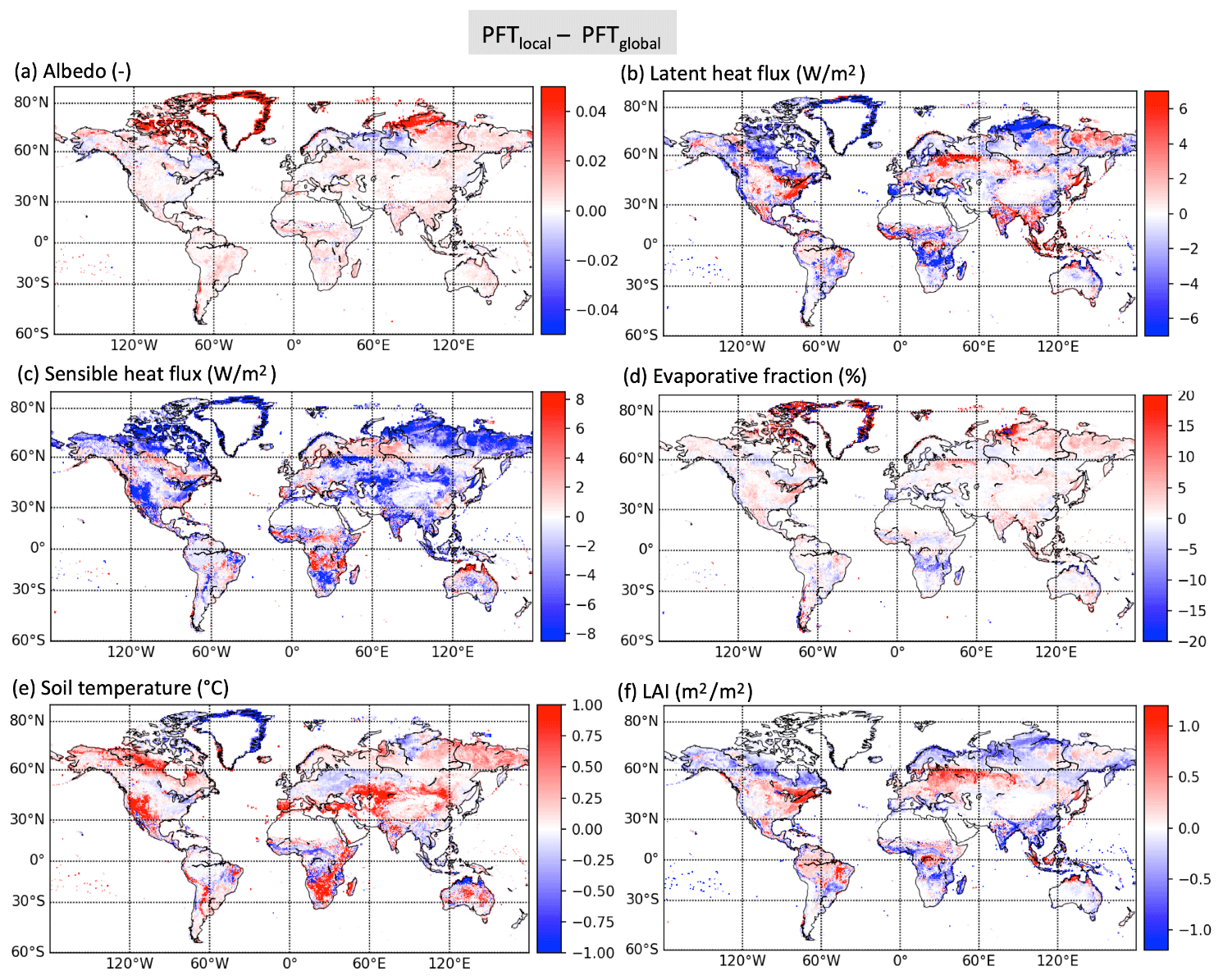
Figure 3Differences in (a) albedo, (b) latent heat flux, (c) sensible heat flux, (d) evaporative fraction – latent heat flux/(latent + sensible heat fluxes) –, (e) soil surface temperature, and (f) leaf area index (LAI) simulated by the ORCHIDEE model between the new PFT (PFTlocal) and old PFT (PFTglobal) distributions for the summer (June–July–August, Northern Hemisphere) of the year 2010.
4.1 ORCHIDEE simulations: new PFT product (PFTlocal) vs. PFT maps based on global CWT (PFTglobal)
In this section, we compare the results of two ORCHIDEE simulations performed, respectively, by applying the old standard PFT maps (PFTglobal) and the new PFT product derived in this study (PFTlocal). The results are shown for the year 2010.
The impacts of the changes in the land surface representation between the local and global PFT maps on the surface albedo, latent and sensible heat fluxes, evaporative fraction (ratio of latent heat flux to the sum of latent and sensible heat fluxes), surface temperature, and the LAI are shown in Fig. 3. Averaged differences (local vs. global) for the Northern Hemisphere summer period (June–July–August, JJA) were plotted here to highlight the main changes, but the plots at the annual scale are also given in Appendix B. The results show that the energy, water, and carbon fluxes are mainly (and significantly) impacted in the regions where woody vegetation was replaced by grasslands or where the bare-soil fraction has changed. Since, in ORCHIDEE, the shrub PFTs are assigned to tree PFTs, the regions highlighted in Sect. 3 with significant fractions of shrub losses or gains in profit of grasses show the largest changes. Given that tree PFTs present a lower albedo, higher roughness (linked to vegetation height) and maximum transpiration capacity, and higher LAI and biomass, the simulated differences between the two simulations show coherent features across the different variables. In summer, surface albedo increases by up to 4 % (absolute deviation) in the northern boreal regions because of the decrease in shrubs and the increase in grasslands and, in some regions (like in the Taymyr Peninsula), the increase in bare soils. South of this boreal zone, both in Eurasia and North America, the increase in trees and decrease in shrubs show opposite variations. In the tropical region (between 0 and 30∘ S), the PFT changes principally concern differences in the shrub–grass partition to the benefit of grasslands. In these regions, the tree fraction decrease results in a slight increase in the albedo around 2 % (absolute deviation). At the annual scale (Fig. B1), the larger impact of the PFT differences at the high latitudes is explained by the cumulative impact of changes in snow cover. Indeed, snowmelt is more rapid on tree cover compared to grasslands, inducing a shorter duration of the snow cover with high albedo values, leading to even more differences between short- and high-vegetation albedo values.
Surface albedo differences (impacting surface net radiation) combined with roughness changes (impacting turbulent exchanges) explain generally the surface flux variations. The balance between the two effects varies according to the latitude following the amount of solar radiation: at the northern latitudes, the impact of surface roughness is larger than at more southerly ones. In the tropics, we observe a decrease in the turbulent fluxes where the albedo is larger, explaining the lower evapotranspiration and lower GPP, with different partitions when comparing arid and humid zones. For example, the consequences of a decrease in shrubs to the benefit of grasses do not have the same effects on the heat flux partition according to the water availability. In regions where soil moisture limits evapotranspiration, like central Africa (south of the Democratic Republic of the Congo) or the Sahel, fewer trees lead to less evapotranspiration of up to 6 Wm−2 in the annual mean and larger sensible heat flux at the same level, whereas at the northern latitudes like in eastern Siberia, fewer shrubs lead to higher evapotranspiration and lower sensible heat flux. This is summarized in the representation of the evaporative fraction, which shows opposite variations in these regions.
The surface temperature, as the result of the energy and water budgets, shows differences in line with the sensible heat flux variations, with larger temperatures where the sensible heat flux has decreased. The differences in summer and in annual mean are significant and can reach 1 K but can show differences of up to 3 K on a daily scale.
LAI differences are in coherence with the PFT differences: lower values where woody vegetation was replaced by grasses, except in eastern Siberia and northern Australia, where the increase in net radiation favoured transpiration, GPP, and, finally, LAI. The LAI variations may reach 1 m2 m−2 in some regions like south-eastern Canada or central Europe, where the broad-leaved deciduous trees have increased in the PFTlocal map.
Figure 4 illustrates the impacts on the above-ground biomass (AGB) with the tree cover variations. To see whether the biomass changes are more realistic, they have been compared to the ESA CCI Biomass product, version 3 (ESACCI Biomass, Santoro and Cartus, 2019; Santoro et al., 2021), aggregated at 0.5∘ resolution. Note that, unlike for the turbulent fluxes discussed above, the change in AGB between low- and high-vegetation covers should be large enough and thus easier to evaluate. In Fig. 4a and b, we first compare the simulated AGB with the new PFTs (PFTlocal) to the ESACCI Biomass product, which highlights some issues related to ORCHIDEE model deficiencies and also, in part, to relatively large errors in the ESACCI Biomass product, especially for high AGB. The model simulates too low AGB on average, with a large underestimation over the tropical forests, which cannot be due to the PFT cover (above 90 % forest cover). Over temperate and high latitudes, we also find significant model AGB underestimation. The improvements/degradations with respect to changing the PFT distribution (Fig. 4d, where the mean errors between the two simulations performed with PFTlocal and PFTglobal are represented) provide contrasting results between regions. The benefits of the new PFTlocal maps (blue colour in Fig. 4d) are visible in north-eastern Europe, the eastern USA, and the Democratic Republic of the Congo, where the increase in tree fraction (Fig. 4c) and biomass seems to be in better agreement with the remote-sensing AGB product. In the other regions, where the tree fractions decreased (northern Canada and Europe, Sahel, Angola, Zambia, and southern China, Fig. 4c), the associated decrease in biomass leads to larger errors compared to the AGB satellite product. In the western USA (California), the losses of tree PFTs to the benefit of grasslands did not impact the simulated biomass since, in these arid regions, the trees have a very low productivity comparable to grasses and thus similar low-biomass values (less than 1 kgC m−2).
Overall, these results highlight the importance and impact of land surface PFT distribution on simulated energy, water, and carbon fluxes as well as carbon stocks in global land surface models.
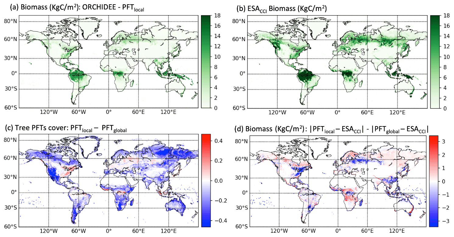
Figure 4Above-ground biomass (AGB) (a) simulated by the ORCHIDEE model with the PFTlocal dataset and (b) observed by the ESACCI Biomass product version v3, for the year 2010 (Santoro and Cartus, 2019). (c) Differences in the tree PFT fraction prescribed. (d) Difference between the mean bias of simulated vs. ESACCI Biomass AGB between the new (PFTlocal) and former (PFTglobal) distributions of PFTs. Negative values indicate a decrease in the bias from PFTglobal to PFTlocal.
4.2 Evaluation of DGVM Joint UK Land Environment Simulator (JULES) – Switch for dynamic vegetation model (TRIFFID) using PFT fractions
The impact of using the new PFT distributions (PFTlocal) as a benchmark for JULES-TRIFFID dynamic vegetation is shown in Fig. 5. In contrast to the results shown in Sect. 4.1, differences found here indicate the value of the new PFT distributions as a product for model evaluation rather than a direct improvement in model predictions. When compared to PFTglobal (“CWT”), JULES-TRIFFID indicates significant overestimation of tree cover in tropical savannas and underestimation of tree cover in boreal north-eastern Russia. Additionally, comparison with the global CWT product (PFTglobal) indicates that JULES-TRIFFID underestimates shrub cover in tropical savannas in South America, Africa, and Australia as well as many semi-arid regions such as western North America. Biases in grass cover are more spatially heterogeneous, but comparison with the global CWT indicates that JULES-TRIFFID strongly overestimates in north-eastern Russia and northern Australia.
When using the new PFT distributions as a benchmark, many of these biases are reduced, as indicated by green areas in column “c” of Fig. 5. In particular, north-eastern boreal Russia shows reduced biases in tree, shrub, and grass cover. Globally, using the new PFT distributions results in a reduction in biases in shrub cover in JULES-TRIFFID in almost every part of the world, particularly savannas and semi-arid regions (Fig. 4d). Whilst no large areas showed a large increase in bias, some areas did show increases in bias of up to 25 %, such as tropical forests (10 % increase), grass cover in tropical savannas (15 % to 25 %) and northern high latitudes (10 % to 20 %), and bare cover in arid regions (up to 10 % increase).
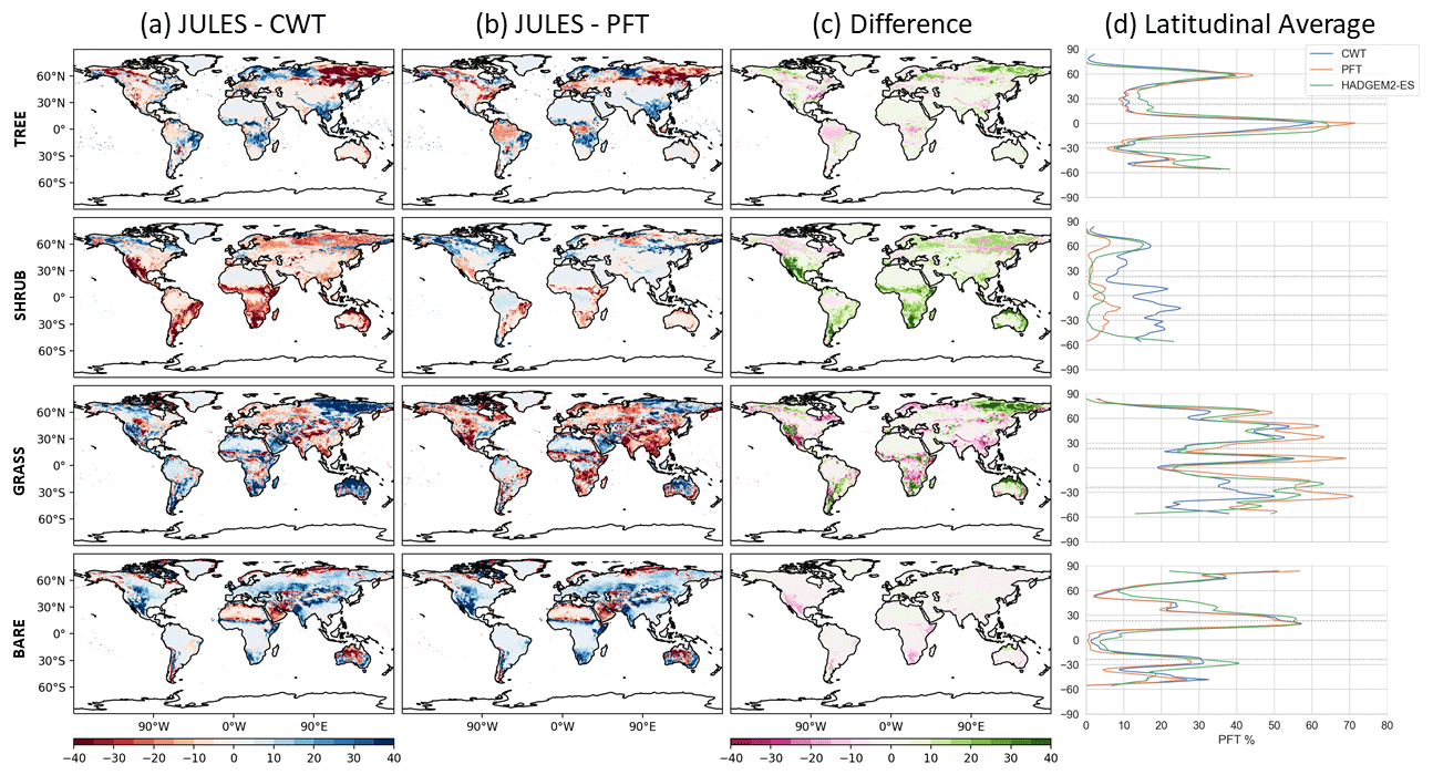
Figure 5Comparison of JULES PFT distributions to both the CWT (PFTglobal) and PFT (PFTlocal) products for major vegetation types. Rows show each major surface type (tree, shrub, grass, bare), whilst the rows show (a) the JULES vegetation distribution compared to the global CWT, (b) the same compared to new PFTlocal distributions, (c) the difference between panels (a) and (b), where green (pink) indicates positive or negative anomalies evaluated closer to 0 (further away from 0) using new PFTlocal distributions, and (d) absolute latitudinal average fractions for each major vegetation type from CWT, PFT, and JULES.
The CCI PFT dataset 1992–2020 is freely, permanently, and publicly available on a web viewer: https://doi.org/10.5285/26a0f46c95ee4c29b5c650b129aab788 (Harper et al., 2023) (http://maps.elie.ucl.ac.be/CCI/viewer/download.php, last access: 20 March 2023).
The new PFT product (PFTlocal) was generated to reduce the cross-walking component of uncertainty by adding spatial variability to the PFT composition within a LC class. This work moved beyond fine-tuning the cross-walking approach for specific LC classes or regions and, instead, separately quantifies the PFT fractional composition for each 300 m pixel globally. The result is a dataset representing the cover fractions of 14 PFTs at 300 m for each year in the 1992–2020 era, consistent with the CCI MRLC map for the corresponding year. The PFTlocal dataset exhibits intra-class spatial variability in PFT fractional cover at the 300 m pixel level and is complementary to the CCI medium-resolution multi-mission LC map series since the derived PFT fractions maintain consistency with the original LC class legend.
The PFTlocal dataset provides a more faithful representation of PFT distributions because it draws on high-resolution peer-reviewed mapping of specific vegetation classes to refine global assumptions about PFT fractions. In many cases, the global CWT presented a reasonable approximation for estimating PFT fractions within many land cover classes, as shown by the fractions estimated from the auxiliary products falling close to those suggested by the global CWT.
Note that a recent study by Marie et al. (2022) followed the same objective of refining the global CWT (used to map the ESA land cover classes onto PFTs) but with a different approach. Instead of using the tree cover dataset from Hansen et al. (2013), they valorized a map of above-ground biomass over Africa (Bouvet et al., 2018) to define local CWTs, using the information from AGB to better constrain the partition between tree and short-vegetation PFTs, for each LC class. As shown in our study, they found that LC class 10 (rain-fed cropland) in the Sahel should contain tree PFTs which correspond to tree crops (Fig. A1). Overall, these efforts highlight the benefits of using additional high-resolution products, like tree cover or AGB, when translating land cover into PFT distributions for land surface models. Merging all sources of information into a coherent PFT product remained however a difficult task. This study demonstrated that using the consistent CCI MRLC time series and maintaining deference to the original LCCS class in the combination rules allowed these auxiliary data to be brought into consistency.
Changing the PFT distribution in the ORCHIDEE model (PFTlocal vs. PFTglobal) induces significant impacts on the simulated water, energy, and carbon fluxes as well as on the modelled carbon stocks. These differences are coherent with changes in surface properties (albedo, roughness, type of cover) induced by changes in PFT types (mainly tree vs. short-vegetation and bare-soil covers). However, it is not possible and is beyond the scope of the paper to evaluate globally and quantitatively model improvements due to changes in PFTs given (i) existing model biases that have been partly compensated by previous model parameter tuning with the old PFT maps (PFTglobal) and (ii) the large uncertainty still associated with data-driven products at a global scale. We initiated an evaluation with AGB; however, the new simulated biomass (induced by PFT changes) is not always closer to the satellite ESACCI AGB product. In addition, the fact that ORCHIDEE does not differentiate between shrubs and trees limits such biomass evaluation. Additional simulations/tests with more models and a more comprehensive evaluation with a larger ensemble of variables and data-driven products are therefore needed to quantify the benefits of the PFTlocal maps.
Using the PFTlocal as a benchmark improves the evaluation of every major surface type in the JULES-TRIFFID dynamic vegetation model, particularly shrub cover. This allows a new perspective on priorities for dynamic vegetation model development.
The user tool described in Poulter et al. (2015) has been reformatted such that it can be applied directly to the new PFT map series to create user-specific ready-to-use inputs for LSMs. The user tool creates model-ready inputs at user specification, which greatly expands the ease of use of the product both within and beyond the modelling community. The PFT dataset is designed primarily for use in land surface and Earth system models. For the vegetated classes except for sparse vegetation, the entire non-water fraction of the 300 m pixel is assigned as vegetation, allowing the actual presence of grass vegetation to be determined by the land surface models. For use outside of modelling, this could introduce some bias (e.g. underestimating bare-soil cover in some pixels and overestimating grass cover), but the fractions of the high-biomass vegetation types (trees and shrubs) can be used for non-modelling use cases.
Production of the PFTlocal product is dependent on the availability and quality of the auxiliary datasets at a spatial resolution higher than 300 m; this is especially critical for mapping the shrubland class. With the combined information of the phenological attribute of the ESA CCI LC classes, the percentage of tree canopy cover from Hansen et al. (2013), and the Global Ecosystem Dynamics Investigation (GEDI) product (Potapov et al., 2021), it was possible, for the first time, to map four shrubland classes at the global scale: broad-leaved evergreen, broad-leaved deciduous, needle-leaved evergreen, and needle-leaved deciduous. However, further research is still needed to improve the estimation of shrubland-class pixels north of 52∘ N (i.e. outside of the extent of the GEDI product). The urban PFT would benefit from separating impervious surfaces from buildings. Finally, the current workflow should further be tested against annual ancillary product updates as operational production of very-high-resolution datasets becomes the norm.
The proposed methodology is automated so that the PFT dataset will be updated annually as new annual land cover maps are produced in C3S. Because the PFT product is harmonized with the CCI MRLC map series, future improvements in the land cover product will flow through to the PFT product.

Figure A1Distribution of tree cover percentage in rain-fed cropland-class pixels in Africa. Grey pixels belong to other classes.

Figure A2Absolute differences (percentage of pixels) between the 2010 PFTlocal dataset and the corresponding PFTglobal maps (i.e. applying the global cross-walking scheme) for the 14 PFT types. The spatial resolution is .
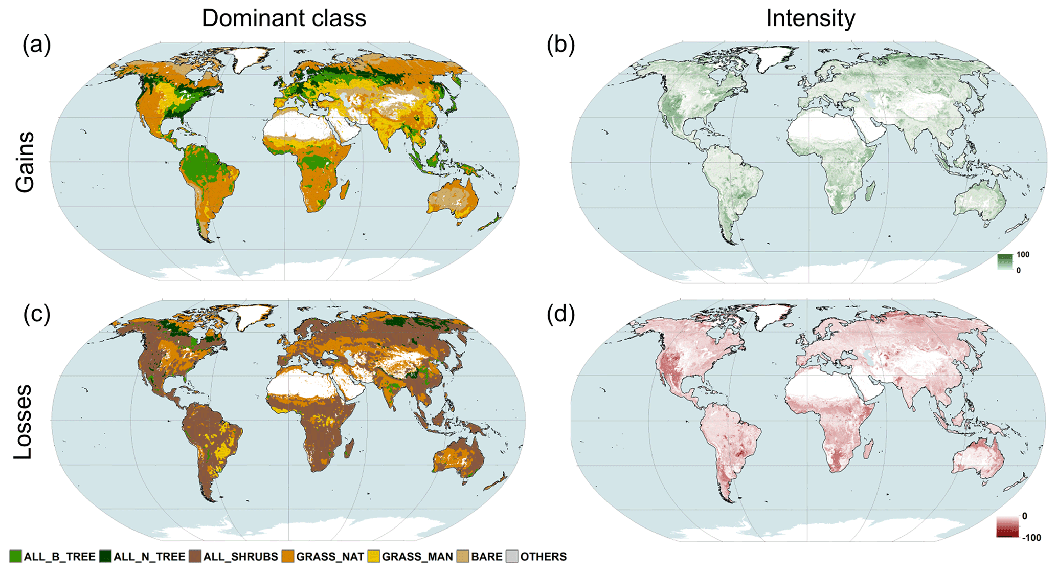
Figure A3PFT with the largest increase (a) and largest loss (c) in coverage within pixels in the PFTlocal dataset compared to the PFTglobal and corresponding fractions gained (b) and lost (d). White areas remained stable in both PFT datasets.
Table A1Global areal cover (1000 km2) of each PFT by land cover class for 2010 based on the most recent version of the global CWT applied to v2.0.8 of the CCI MRLC map.
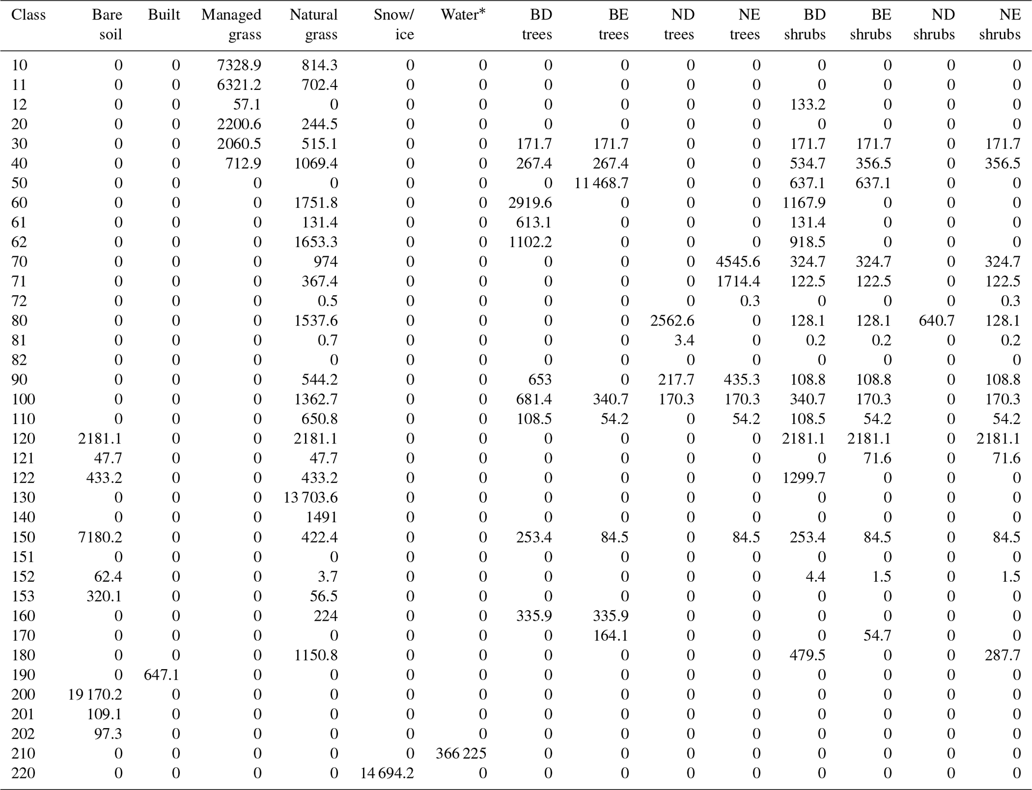
* For the water body class (code 210), the water PFT area includes 3 110 600 km2 of inland water.
Table A2Percentage PFT composition by class based on the most recent update to the global cross-walking table.
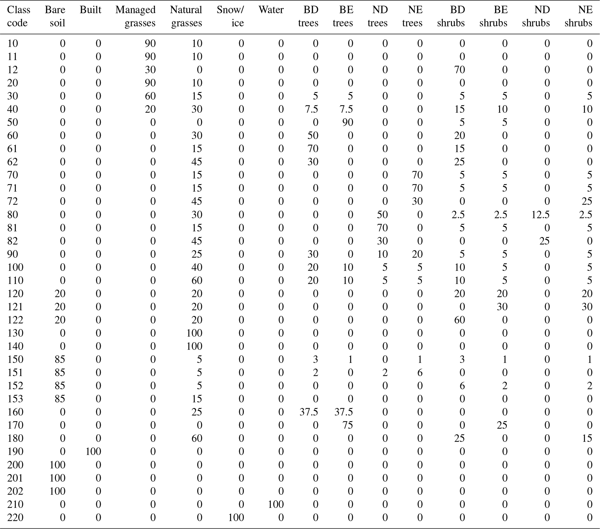
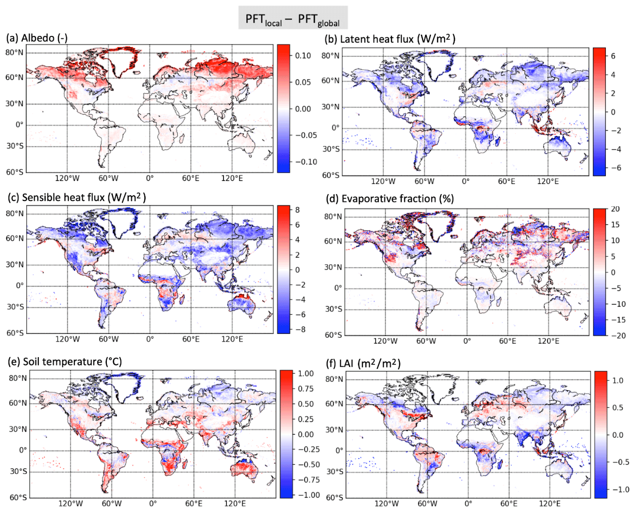
Figure B1Differences in albedo (a), latent heat flux (b), sensible heat flux (c), evaporative fraction d – latent heat flux/latent + sensible heat fluxes, soil surface temperature (e) and leaf area index (LAI, f) simulated by the ORCHIDEE model between the new PFT and old PFT distributions for the annual mean of the year 2010 (same as Fig. 4 but for the annual mean).
Table C1Default land cover to plant functional type cross-walking table provided by the conversion tool with the level-1 UN LCCS classes and level-2 UN LCCS sub-classes in italics. The units are percentage coverage of each PFT per UN LCCS class (from Poulter et al., 2015).
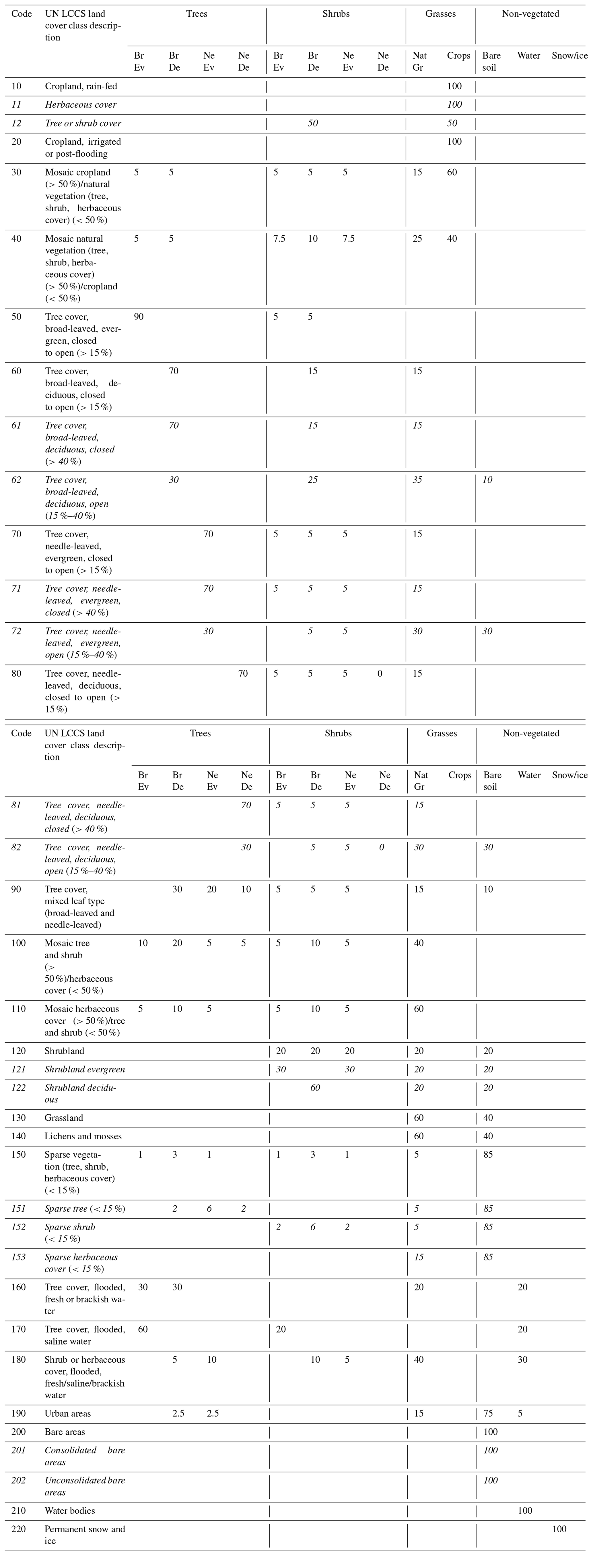
PD conceived the idea and supervised the research effort with contributions from PP. CL coordinated the project. KLH designed the methodology with the contribution of CL. KLH developed the code to generate the CCI PFT dataset 2010. AH, PP, CO, VB, RSM, and SIB designed the modelling experiments and analysed the results. GK, MB, RS, and CB designed and developed the user tool. GK and RS managed and produced the CCI PFT dataset 2010 metadata. KLH wrote the original draft with contributions from CL, AH, SIB, PP, and CO. All the co-authors reviewed the manuscript.
The contact author has declared that none of the authors has any competing interests.
Publisher’s note: Copernicus Publications remains neutral with regard to jurisdictional claims in published maps and institutional affiliations.
The study was carried out in the framework of the European Space Agency Climate Change Initiative (ESA CCI). The ESA CCI supported the methodological development and generation of the global PFT map series 1992–2020 as well as the climate modelling analysis. We thank Olivier Arino and Fabrizio Ramoino for their long-term support in the Land_Cover_cci project. We thank Clement Albergel for his fresh look at the work done and his review. We thank Benjamin Goffart for tailoring the CCI Land Cover web interface to visualize and interact with the CCI PFT dataset 2010.
This research has been supported by the European Space Agency (grant no. ESA/No.4000126564).
This paper was edited by Jia Yang and reviewed by two anonymous referees.
Andréfouët, S., Bindschadler, R., Brown De Colstoun, E. C., Choate, M., Chomentowski, W., Christopherson, J., Doorn, B., Hall, D. K., Holifield, C., Howard, S., Kranenburg, C., Lee, S., Masek, J. B., Moran, M., Mueller-Karger, F., Ohlen, D., Palandro, D., Price, J., Qi, J., Reed, B. C., Samek, J., Scaramuzza, P., Skole, D., Schott, J., Storey, J., Thome, K., Torres-Pulliza, D., Vogelmann, J., Williams, D. L., Woodcock, C., and Wylie, B.: Preliminary Assessment of the Value of Landsat-7 ETM+ Data Following Scan Line Corrector Malfunction, US Geological Survey, EROS Data Center: Sioux Falls, SD, USA, Science, 1–86, 2003.
Bartsch, A., Widhalm, B., Pointner, G., Ermokhina, K. A., Leibman, M., and Heim, B.: Land cover derived from Sentinel-1 and Sentinel-2 satellite data (2015–2018) for subarctic and arctic environments, Zentralanstalt für Meteorologie und Geodynamik, Wien, PANGAEA, https://doi.org/10.1594/PANGAEA.897916, 2019.
Bastos, A., O'Sullivan, M., Ciais, P., Makowski, D., Sitch, S., Friedlingstein, P., Chevallier, F., Rödenbeck, C., Pongratz, J., Luijkx, I. T., Patra, P. K., Peylin, P., Canadell, J. G., Lauerwald, R., Li, W., Smith, N. E., Peters, W., Goll, D. S., Jain, A. K., Kato, E., Lienert, S., Lombardozzi, D. L., Haverd, V., Nabel, J. E. M. S., Poulter, B., Tian, H., Walker, A. P., and Zaehle, S.: Sources of uncertainty in regional and global terrestrial CO2 exchange estimates, Global Biogeochem. Cy., 34, 1–21, https://doi.org/10.1029/2019GB006393, 2020.
Bastos, A., Hartung, K., Nützel, T. B., Nabel, J. E. M. S., Houghton, R. A., and Pongratz, J.: Comparison of uncertainties in land-use change fluxes from bookkeeping model parameterisation, Earth Syst. Dynam., 12, 745–762, https://doi.org/10.5194/esd-12-745-2021, 2021.
Beck, H. E., Zimmermann, N. E., McVicar, T. R., Vergopolan, N., Berg, A., and Wood, E. F.: Present and future Köppen-Geiger climate classification maps at 1-km resolution, Nature Scientific Data, 5, 180214, https://doi.org/10.1038/sdata.2018.214, 2018.
Best, M. J., Pryor, M., Clark, D. B., Rooney, G. G., Essery, R. L. H., Ménard, C. B., Edwards, J. M., Hendry, M. A., Porson, A., Gedney, N., Mercado, L. M., Sitch, S., Blyth, E., Boucher, O., Cox, P. M., Grimmond, C. S. B., and Harding, R. J.: The Joint UK Land Environment Simulator (JULES), model description – Part 1: Energy and water fluxes, Geosci. Model Dev., 4, 677–699, https://doi.org/10.5194/gmd-4-677-2011, 2011.
Bouvet, A., Mermoz, S., Le Toan, T., Villard, L., Mathieu, R., Naidoo, L., and Asner, G. P.: An Above-Ground Biomass Map of African Savannahs and Woodlands at 25 m Resolution Derived from ALOS PALSAR, Remote Sens. Environ., 206, 156–173, https://doi.org/10.1016/j.rse.2017.12.030, 2018.
Box, E. O.: Predicting physiognomic vegetation types with climate variables, Vegetatio, 45, 127–139, https://doi.org/10.1007/BF00119222, 1981.
Box, E. O.: Plant functional types and climate at the global scale, J. Veg. Sci., 7, 309–320, https://doi.org/10.2307/3236274, 1996.
Brovkin, V., Claussen, M., Driesschaert, E., Fichefet, T., Kicklighter, D., Loutre, M. F., Matthews, H. D., Ramankutty, N., Schaeffer, M., and Sokolov, A.: Biogeophysical effects of historical land cover changes simulated by six Earth system models of intermediate complexity, Clim. Dynam., 26, 587–600, https://doi.org/10.1007/s00382-005-0092-6, 2006.
Clark, D. B., Mercado, L. M., Sitch, S., Jones, C. D., Gedney, N., Best, M. J., Pryor, M., Rooney, G. G., Essery, R. L. H., Blyth, E., Boucher, O., Harding, R. J., Huntingford, C., and Cox, P. M.: The Joint UK Land Environment Simulator (JULES), model description – Part 2: Carbon fluxes and vegetation dynamics, Geosci. Model Dev., 4, 701–722, https://doi.org/10.5194/gmd-4-701-2011, 2011.
Dale, V. H.: The relationship between land-use change and climate change, Ecol. Appl., 7, 753–769, https://doi.org/10.1890/1051-0761(1997)007[0753:TRBLUC]2.0.CO;2, 1997.
Danielson, J. and Gesch, D.: Global Multi-resolution Terrain Elevation Data 2010 (GMTED2010), U.S. Geological Survey Open File Report 2011–1073, US Department of the Interior, US Geological Survey Washington, DC, USA, https://doi.org/10.3133/ofr20111073, 2011.
Defourny, P., Lamarche, C., Brockmann, C., Boettcher, M., Bontemps, S., De Maet, T., Duveiller, G. L. Harper, K., Hartley A., Kirches, G., Moreau, I., Peylin, P., Ottlé, C., Radoux J., Van Bogaert, E., Ramoino, F., Albergel, C., and Arino, O.: Observed annual global land-use change from 1992 to 2020 three times more dynamic than reported by inventory-based statistics, in preparation, 2023.
Devaraju, N., Bala, G., and Modak, A.: Effects of large-scale deforestation on precipitation in the monsoon regions: Remote versus local effects, P. Natl. Acad. Sci. USA, 112, 3257–3262, https://doi.org/10.1073/pnas.1423439112, 2015.
Di Gregorio, A., and Jansen, L. J. M. Land Cover Classification System (LCCS): Classification Concepts and User Manual, Fao, Vol. 53, Food & Agriculture Organization, https://www.fao.org/3/x0596e/x0596e00.htm (last access: 20 March 2023), 2005.
Esch, T., Heldens, W., Hirner, A., Keil, M., Marconcini, M., Roth, A., Zeidler, J., Dech, S., and Strano, E.: Breaking new ground in mapping human settlements from space – The Global Urban Footprint, J. Photogramm. Remote, 134, 30–42, https://doi.org/10.1016/j.isprsjprs.2017.10.012, 2017.
Feddema, J., Oleson, K., Bonan, G., Mearns, L., Washington, W., Meehl, G., and Nychka, D.: A comparison of a GCM response to historical anthropogenic land cover change and model sensitivity to uncertainty in present-day land cover representations, Clim. Dynam., 25, 581–609, https://doi.org/10.1007/s00382-005-0038-z, 2005.
Foley, J. A., DeFries, R., Asner, G. P., Barford, C., Bonan, G., Carpenter, S. R., Chapin, F. S., Coe, M. T., Daily, G. C., Gibbs, H. K., Helkowski, J. H., Holloway, T., Howard, E. A., Kucharik, C. J., Monfreda, C., Patz, J. A., Prentice, I. C., Ramankutty, N., and Snyder, P. K.: Global consequences of land use, Science, 309, 570–574, https://doi.org/10.1126/science.1111772, 2005.
Friedlingstein, P., Jones, M. W., O'Sullivan, M., Andrew, R. M., Bakker, D. C. E., Hauck, J., Le Quéré, C., Peters, G. P., Peters, W., Pongratz, J., Sitch, S., Canadell, J. G., Ciais, P., Jackson, R. B., Alin, S. R., Anthoni, P., Bates, N. R., Becker, M., Bellouin, N., Bopp, L., Chau, T. T. T., Chevallier, F., Chini, L. P., Cronin, M., Currie, K. I., Decharme, B., Djeutchouang, L. M., Dou, X., Evans, W., Feely, R. A., Feng, L., Gasser, T., Gilfillan, D., Gkritzalis, T., Grassi, G., Gregor, L., Gruber, N., Gürses, Ö., Harris, I., Houghton, R. A., Hurtt, G. C., Iida, Y., Ilyina, T., Luijkx, I. T., Jain, A., Jones, S. D., Kato, E., Kennedy, D., Klein Goldewijk, K., Knauer, J., Korsbakken, J. I., Körtzinger, A., Landschützer, P., Lauvset, S. K., Lefèvre, N., Lienert, S., Liu, J., Marland, G., McGuire, P. C., Melton, J. R., Munro, D. R., Nabel, J. E. M. S., Nakaoka, S.-I., Niwa, Y., Ono, T., Pierrot, D., Poulter, B., Rehder, G., Resplandy, L., Robertson, E., Rödenbeck, C., Rosan, T. M., Schwinger, J., Schwingshackl, C., Séférian, R., Sutton, A. J., Sweeney, C., Tanhua, T., Tans, P. P., Tian, H., Tilbrook, B., Tubiello, F., van der Werf, G. R., Vuichard, N., Wada, C., Wanninkhof, R., Watson, A. J., Willis, D., Wiltshire, A. J., Yuan, W., Yue, C., Yue, X., Zaehle, S., and Zeng, J.: Global Carbon Budget 2021, Earth Syst. Sci. Data, 14, 1917–2005, https://doi.org/10.5194/essd-14-1917-2022, 2022.
Frieler, K., Lange, S., Piontek, F., Reyer, C. P. O., Schewe, J., Warszawski, L., Zhao, F., Chini, L., Denvil, S., Emanuel, K., Geiger, T., Halladay, K., Hurtt, G., Mengel, M., Murakami, D., Ostberg, S., Popp, A., Riva, R., Stevanovic, M., Suzuki, T., Volkholz, J., Burke, E., Ciais, P., Ebi, K., Eddy, T. D., Elliott, J., Galbraith, E., Gosling, S. N., Hattermann, F., Hickler, T., Hinkel, J., Hof, C., Huber, V., Jägermeyr, J., Krysanova, V., Marcé, R., Müller Schmied, H., Mouratiadou, I., Pierson, D., Tittensor, D. P., Vautard, R., van Vliet, M., Biber, M. F., Betts, R. A., Bodirsky, B. L., Deryng, D., Frolking, S., Jones, C. D., Lotze, H. K., Lotze-Campen, H., Sahajpal, R., Thonicke, K., Tian, H., and Yamagata, Y.: Assessing the impacts of 1.5 °C global warming – simulation protocol of the Inter-Sectoral Impact Model Intercomparison Project (ISIMIP2b), Geosci. Model Dev., 10, 4321–4345, https://doi.org/10.5194/gmd-10-4321-2017, 2017.
GCOS (Global Climate Observing System): Public Review of GCOS Requirements for Essential Climate Variables Survey, GCOS Review of Requirements for Climate Monitoring, https://gcos.wmo.int/en/essential-climate-variables/table (last access: 20 March 2023), 2016.
Hansen, M. C., Potapov, P. V., Moore, R., Hancher, M., Turubanova, S. A., Tyukavina, A., Thau, D., Stehman, S. V., Goetz, S. J., Loveland, T. R., Kommareddy, A., Egorov, A., Chini, L., Justice, C. O., and Townshend, J. R. G.: High-resolution global maps of 21st-century forest cover change, Science, 342, 850–853, https://doi.org/10.1126/science.1244693, 2013.
Harper, K. L., Lamarche, C., Hartley, A., Peylin, P., Ottlé, C., Bastrikov, V., San Martín, R., Bohnenstengel, S. I., Kirches, G., Boettcher, M., Shevchuk, R., Brockmann, C., and Defourny, P.: ESA Land Cover Climate Change Initiative (Land_Cover_cci): Global Plant Functional Types (PFT) Dataset, v2.0.8, NERC EDS Centre for Environmental Data Analysis [data set], https://doi.org/10.5285/26a0f46c95ee4c29b5c650b129aab788, 2023.
Harris, I., Jones, P. D., Osborn, T. J., and Lister, D. H.: Updated high-resolution grids of monthly climatic observations – the CRU TS3.10 Dataset, Int. J. Climatol., 34, 623–642, https://doi.org/10.1002/joc.3711, 2014.
Hartley, A. J., MacBean, N., Georgievski, G., and Bontemps, S.: Uncertainty in plant functional type distributions and its impact on land surface models, Remote Sens. Environ., 2013, 71–89, https://doi.org/10.1016/j.rse.2017.07.037, 2017.
Hollmann, R., Merchant, C. J., Saunders, R., Downy, C., Buchwitz, M., Cazenave, A., Chuvieco, E., Defourny, P., De Leeuw, G., Forsberg, R., Holzer-Popp, T., Paul, F., Sandven, S., Sathyendranath, S., Van Roozendael, M., Wagner, W., others, Holzer-Popp, T., Paul, F., Sandven, S., Sathyendranath, S., Van Roozendael, M., and Wagner, W.: The ESA climate change initiative: Satellite data records for essential climate variables, B. Am. Meteorol. Soc., 94, 1541–1552, https://doi.org/10.1175/BAMS-D-11-00254.1, 2013.
Houghton, R. A.: Aboveground forest biomass and the global carbon balance, Glob. Change Biol., 11, 945–958, https://doi.org/10.1111/j.1365-2486.2005.00955.x, 2005.
Houghton, R. A., House, J. I., Pongratz, J., van der Werf, G. R., DeFries, R. S., Hansen, M. C., Le Quéré, C., and Ramankutty, N.: Carbon emissions from land use and land-cover change, Biogeosciences, 9, 5125–5142, https://doi.org/10.5194/bg-9-5125-2012, 2012.
IPCC: Climate Change 2022: Impacts, Adaptation, and Vulnerability. Contribution of Working 744 Group II to the Sixth Assessment Report of the Intergovernmental Panel on Climate Change, edited by: Pörtner, O., Roberts, D. C., Tignor, M., Poloczanska, E. S., Mintenbeck, K., and Ale, A., 2022.
Jung, M., Henkel, K., Herold, M., and Churkina, G.: Exploiting synergies of global land cover products for carbon cycle modeling, Remote Sens. Environ., 101, 534–553, https://doi.org/10.1016/j.rse.2006.01.020, 2006.
Kobayashi, S., Ota, Y., Harada, Y., Ebita, A., Moriya, M., Onoda, H., Onogi, K., Kamahori, H., Kobayashi, C., Endo, H., Miyaoka, K., and Takahashi, K.: The JRA-55 Reanalysis: General Specifications and Basic Characteristics, J. Meteorol. Soc. Jpn., 93, 5–48, https://doi.org/10.2151/jmsj.2015-001, 2015.
Krinner, G., Viovy, N., de Noblet-Ducoudré, N., Ogée, J., Polcher, J., Friedlingstein, P., Ciais, P., Sitch, S., and Prentice, I. C.: A dynamic global vegetation model for studies of the coupled atmosphere-biosphere system, Global Biogeochem. Cy., 19, 1–33, https://doi.org/10.1029/2003GB002199, 2005.
Lamarche, C., Santoro, M., Bontemps, S., d'Andrimont, R., Radoux, J., Giustarini, L., Brockmann, C., Wevers, J., Defourny, P., and Arino, O.: Compilation and validation of sar and optical data products for a complete and global map of inland/ocean water tailored to the climate modeling community, 9, Remote Sens., https://doi.org/10.3390/rs9010036, 2017.
Lambin, E. F., Turner, B. L., Geist, H. J., Agbola, S. B., Angelsen, A., Bruce, J. W., Coomes, O. T., Dirzo, R., Fischer, G., Folke, C., George, P. S., Homewood, K., Imbernon, J., Leemans, R., Li, X., Moran, E. F., Mortimore, M., Ramakrishnan, P. S., Richards, J. F., Skånes, H., Steffen, W., Stone, G. D., Svedin, U., Veldkamp, T. A., Vogel, C., and Xu, J.: The causes of land-use and land-cover change: Moving beyond the myths, Global Environ. Chang., 11, 261–269, https://doi.org/10.1016/S0959-3780(01)00007-3, 2001.
Liu, S., Bond-Lamberty, B., Boysen, L. R., Ford, J. D., Fox, A., Gallo, K., Hatfield, J., Henebry, G. M., Huntington, T. G., Liu, Z., Lovelan, T. R., Norby, R. J., Soh, T., Steiner, A. L., Yuan, W., Zhang, Z., and Zhao, S.: Grand challenges in understanding the interplay of climate and land changes, Earth Interact., 21, 1–43, https://doi.org/10.1175/EI-D-16-0012.1, 2017.
Loarie, S. R., Lobell, D. B., Asner, G. P., and Field, C. B.: Land-Cover and surface water change drive large albedo increases in south america, Earth Interact., 15, 1–16, https://doi.org/10.1175/2010EI342.1, 2011.
Lurton, T., Balkanski, Y., Bastrikov, V., Bekki, S., Bopp, L., Braconnot, P., Brockmann, P., Cadule, P., Contoux, C., Cozic, A., Cugnet, D., Dufresne, J. L., Éthé, C., Foujols, M. A., Ghattas, J., Hauglustaine, D., Hu, R. M., Kageyama, M., Khodri, M., Lebas, N., Levavasseur, G., Marchand, M., Ottlé, C., Peylin, P., Sima, A., Szopa, S., Thiéblemont, R., Vuichard, N., and Boucher, O.: Implementation of the CMIP6 Forcing Data in the IPSL-CM6A-LR Model, J. Adv. Model. Earth Sy., 12, 1–22, https://doi.org/10.1029/2019MS001940, 2020.
Mahmood, R., Pielke, R. A., Hubbard, K. G., Niyogi, D., Dirmeyer, P. A., Mcalpine, C., Carleton, A. M., Hale, R., Gameda, S., Beltrán-Przekurat, A., Baker, B., Mcnider, R., Legates, D. R., Shepherd, M., Du, J., Blanken, P. D., Frauenfeld, O. W., Nair, U. S., and Fall, S.: Land cover changes and their biogeophysical effects on climate, Int. J. Climatol., 34, 929–953, https://doi.org/10.1002/joc.3736, 2014.
Marie, G., Luyssaert, B. S., Dardel, C., Le Toan, T., Bouvet, A., Mermoz, S., Villard, L., Bastrikov, V., and Peylin, P.: Constraining a land cover map with satellite-based aboveground biomass estimates over Africa, Geosci. Model Dev., 15, 2599–2617, https://doi.org/10.5194/gmd-15-2599-2022, 2022.
Mathison, C., Burke, E., Hartley, A. J., Kelley, D. I., Burton, C., Robertson, E., Gedney, N., Williams, K., Wiltshire, A., Ellis, R. J., and others: Description and Evaluation of the JULES-ES setup for ISIMIP2b, EGUsphere, 1–24, 2022.
McGlynn, E., Li, S., Berger, M. F., Amend, M., and Harper, K. L.: Addressing uncertainty and bias in land use, land use change, and forestry greenhouse gas inventories, Clim. Change, 170, 1–25, https://doi.org/10.1007/s10584-021-03254-2, 2022.
Pachauri, R. K., Allen, M. R., Barros, V. R., Broome, J., Cramer, W., Christ, R., Church, J. A., Clarke, L., Dahe, Q., Dasgupta, P., Dubash, N. K., Edenhofer, O., Elgizouli, I., Field, C. B., Forster, P., Friedlingstein, P., Fuglestvedt, J., Gomez-Echeverri, L., Hallegatte, S., Hegerl, G., Howden, M., Jiang, K., Jimenez Cisneroz, B., Kattsov, V., Lee, H., Mach, K. J., Marotzke, J., Mastrandrea, M. D., Meyer, L., Minx, J., Mulugetta, Y., O'Brien, K., Oppenheimer, M., Pereira, J. J., Pichs-Madruga, R., Plattner, G. K., Pörtner, H. O., Power, S. B., Preston, B., Ravindranath, N. H., Reisinger, A., Riahi, K., Rusticucci, M., Scholes, R., Seyboth, K., Sokona, Y., Stavins, R., Stocker, T. F., Tschakert, P., van Vuuren, D., and van Ypserle, J. P.: Climate Change 2014: Synthesis Report, Contribution of Working Groups I, II and III to the Fifth Assessment Report of the Intergovernmental Panel on Climate Change, edited by: Pachauri, R. and Meyer, L., Geneva, Switzerland, IPCC, 151 p., ISBN 978-92-9169-143-2, 2014.
Pekel, J.-F., Cottam, A., Gorelick, N., and Belward, A. S.: High-resolution mapping of global surface water and its long-term changes, Nature, 540, 418–422, https://doi.org/10.1038/nature20584, 2016.
Perugini, L., Caporaso, L., Marconi, S., Cescatti, A., Quesada, B., De Noblet-Ducoudré, N., House, J. I., and Arneth, A.: Biophysical effects on temperature and precipitation due to land cover change, Environ. Res. Lett., 12, https://doi.org/10.1088/1748-9326/aa6b3f, 2017.
Pesaresi, M., Huadong, G., Blaes, X., Ehrlich, D., Ferri, S., Gueguen, L., Halkia, M., Kauffmann, M., Kemper, T., Lu, L., Marin-Herrera, M. A., Ouzounis, G. K., Scavazzon, M., Soille, P., Syrris, V., and Zanchetta, L.: A global human settlement layer from optical HR/VHR RS data: Concept and first results, IEEE J. Sel. Top. Appl., 6, 2102–2131, https://doi.org/10.1109/JSTARS.2013.2271445, 2013.
Pielke, R. A.: Land use and climate change, Science, 310, 1625–1626, https://doi.org/10.1126/science.1120529, 2005.
Pielke, R. A., Pitman, A., Niyogi, D., Mahmood, R., McAlpine, C., Hossain, F., Goldewijk, K. K., Nair, U., Betts, R., Fall, S., Reichstein, M., Kabat, P., and de Noblet, N.: Land use/land cover changes and climate: Modeling analysis and observational evidence, Wiley Interdiscip. Rev. Clim. Chang., 2, 828–850, https://doi.org/10.1002/wcc.144, 2011.
Pitman, A. J., De Noblet-Ducoudré, N., Cruz, F. T., Davin, E. L., Bonan, G. B., Brovkin, V., Claussen, M., Delire, C., Ganzeveld, L., Gayler, V., Van Den Hurk, B. J. J. M., Lawrence, P. J., Van Der Molen, M. K., Müller, C., Reick, C. H., Seneviratne, S. I., Strengen, B. J., and Voldoire, A.: Uncertainties in climate responses to past land cover change: First results from the LUCID intercomparison study, Geophys. Res. Lett., 36, 1–6, https://doi.org/10.1029/2009GL039076, 2009.
Plummer, S., Lecomte, P., and Doherty, M.: The ESA Climate Change Initiative (CCI): A European contribution to the generation of the Global Climate Observing System, Remote Sens. Environ., 203, 2–8, https://doi.org/10.1016/j.rse.2017.07.014, 2017.
Pongratz, J., Reick, C. H., Houghton, R. A., and House, J. I.: Terminology as a key uncertainty in net land use and land cover change carbon flux estimates, Earth Syst. Dynam., 5, 177–195, https://doi.org/10.5194/esd-5-177-2014, 2014.
Potapov, P., Li, X., Hernandez-Serna, A., Tyukavina, A., Hansen, M.C., Kommareddy, A., Pickens, A., Turubanova, S., Tang, H., Edibaldo Silva, C., Armston, J., Dubayah, R., Blair, J. B., and Hofton, M.: Mapping global forest canopy height through integration of GEDI and Landsat data, Remote Sens. Environ., 253, 112165, https://doi.org/10.1016/j.rse.2020.112165, 2021.
Poulter, B., Ciais, P., Hodson, E., Lischke, H., Maignan, F., Plummer, S., and Zimmermann, N. E.: Plant functional type mapping for earth system models, Geosci. Model Dev., 4, 993–1010, https://doi.org/10.5194/gmd-4-993-2011, 2011.
Poulter, B., MacBean, N., Hartley, A., Khlystova, I., Arino, O., Betts, R., Bontemps, S., Boettcher, M., Brockmann, C., Defourny, P., Hagemann, S., Herold, M., Kirches, G., Lamarche, C., Lederer, D., Ottlé, C., Peters, M., and Peylin, P.: Plant functional type classification for earth system models: results from the European Space Agency's Land Cover Climate Change Initiative, Geosci. Model Dev., 8, 2315–2328, https://doi.org/10.5194/gmd-8-2315-2015, 2015.
Sampaio, G., Nobre, C., Costa, M. H., Satyamurty, P., Soares-Filho, B. S., and Cardoso, M.: Regional climate change over eastern Amazonia caused by pasture and soybean cropland expansion, Geophys. Res. Lett., 34, 2007.
Santoro, M. and Cartus, O.: ESA Biomass Climate Change Initiative (Biomass_cci): Global datasets of forest above-ground biomass for the year 2017, v1, Centre for Environmental Data Analysis, https://doi.org/10.5285/bedc59f37c9545c981a839eb552e4084, 2019.
Santoro, M., Cartus, O., Carvalhais, N., Rozendaal, D. M. A., Avitabile, V., Araza, A., de Bruin, S., Herold, M., Quegan, S., Rodríguez-Veiga, P., Balzter, H., Carreiras, J., Schepaschenko, D., Korets, M., Shimada, M., Itoh, T., Moreno Martínez, Á., Cavlovic, J., Cazzolla Gatti, R., da Conceição Bispo, P., Dewnath, N., Labrière, N., Liang, J., Lindsell, J., Mitchard, E. T. A., Morel, A., Pacheco Pascagaza, A. M., Ryan, C. M., Slik, F., Vaglio Laurin, G., Verbeeck, H., Wijaya, A., and Willcock, S.: The global forest above-ground biomass pool for 2010 estimated from high-resolution satellite observations, Earth Syst. Sci. Data, 13, 3927–3950, https://doi.org/10.5194/essd-13-3927-2021, 2021.
Sayre, R., Dangermond, J., Frye, C., Vaughan, R., Aniello, P., Breyer, S., Cribbs, D., Hopkins, D., Nauman, R., Derrenbacher, W., Wright, D., Brown, C., Convis, C., Smith, J., Benson, L., VanSistine, D.P., Warner, H., Cress, J., Danielson, J., Hamann, S., Cecere, T., Reddy, A., Burton, D., Grosse, A., True, D., Metzger, M., Hartmann, J., N. Moosdorf, N., Dürr, H., Paganini, M., Defourny, P., Arino, O., Maynard, S., Anderson, M., and Comer, P.: A New Map of Global Ecological Land Units – An Ecophysiographic Stratification Approach, Association of American Geographers, Washington, DC, ISBN 978-0-89291-276-6, 2014.
Sessa, R.: Terrestrial Essential Climate Variables: For Climate Change Assessment, Mitigation and Adaptation, FAO, edited by: Dolman, H., Rome: GTOS-Secr., Food and Agriculture Organization of the United Nations, https://www.fao.org/3/i0197e/i0197e.pdf (last access: 20 March 2023), 2008.
Stehfest, E., van Vuuren, D., Kram, T., Bouwman, L., Alkemade, R., Bakkenes, M., Biemans, H., Bouwman, A., den Elzen, M., Janse, J., Lucas, P., van Minnen, J., Müller, C., and Prins, A. G.: Integrated Assessment of Global Environmental Change with IMAGE 3.0. Model description and policy applications, 370 pp., Netherlands Environmental Assessment Agency (PBL), 2014.
Turner, B. L., Moss, R. H., and Skole, D. L.: Relating land use and global land-cover change: a proposal for an IGBP-HDP core project, A report from the IGBP/HDP Working Group on Land-Use/Land-Cover Change, Stockholm: Royal Swedish Academy of Scie, IGBP Secretariat, 65 pp., 1993.
UNFCCC: Annex to Report of the Conference of the Parties on its twenty-first session, held in Paris from 30 November to 13 December 2015, Addendum. Part two: Action taken by the Conference of the Parties at its twenty-first session, FCCC/CP/2015/10/Add.1 pp., 2016.
University of East Anglia Climatic Research Unit and Harris, I. C.: CRU JRA v2.0: A forcings dataset of gridded land surface blend of Climatic Research Unit (CRU) and Japanese reanalysis (JRA) data, January 1901–December 2018, Centre for Environmental Data Analysis, https://catalogue.ceda.ac.uk/uuid/7f785c0e80aa4df2b39d068ce7351bbb (last access: 20 March 2023), 2019.
Vitousek, P. M., Ehrlich, P. R., Ehrlich, A. H., and Matson, P. A.: Human Appropriation of the Products of Photosynthesis, Bioscience, 36, 368–373, 1986.
- Abstract
- Introduction
- Methods
- CCI PFT dataset description
- Modelling results
- Data availability
- Conclusion and perspectives
- Appendix A: Complementary information about the CCI PFT dataset description
- Appendix B: Complementary information about the modelling results
- Appendix C: The original default land cover to plant functional type cross-walking table
- Author contributions
- Competing interests
- Disclaimer
- Acknowledgements
- Financial support
- Review statement
- References