the Creative Commons Attribution 4.0 License.
the Creative Commons Attribution 4.0 License.
 | 31 Mar 2023
EURADCLIM: the European climatological high-resolution gauge-adjusted radar precipitation dataset
Else van den Besselaar
Gerard van der Schrier
Jan Fokke Meirink
Emiel van der Plas
Hidde Leijnse
The European climatological high-resolution gauge-adjusted radar precipitation dataset, EURADCLIM, addresses the need for an accurate (sub)daily precipitation product covering 78 % of Europe at a high spatial resolution. A climatological dataset of 1 and 24 h precipitation accumulations on a 2 km grid is derived for the period 2013 through 2020. The starting point is the European Meteorological Network (EUMETNET) Operational Program on the Exchange of Weather Radar Information (OPERA) gridded radar dataset of 15 min instantaneous surface rain rates, which is based on data from, on average, 138 ground-based weather radars. First, methods are applied to further remove non-meteorological echoes from these composites by applying two statistical methods and a satellite-based cloud-type mask. Second, the radar composites are merged with the European Climate Assessment & Dataset (ECA&D) with potentially ∼ 7700 rain gauges from National Meteorological and Hydrological Services (NMHSs) in order to substantially improve its quality. Characteristics of the radar, rain gauge and satellite datasets are presented, as well as a detailed account of the applied algorithms. The clutter-removal algorithms are effective while removing few precipitation echoes. The usefulness of EURADCLIM for quantitative precipitation estimation (QPE) is confirmed by comparison against rain gauge accumulations employing scatter density plots, statistical metrics and a spatial verification. These show a strong improvement with respect to the original OPERA product. The potential of EURADCLIM to derive pan-European precipitation climatologies and to evaluate extreme precipitation events is shown. Specific attention is given to the remaining artifacts in and limitations of EURADCLIM. Finally, it is recommended to further improve EURADCLIM by applying algorithms to 3D instead of 2D radar data and by obtaining more rain gauge data for the radar–gauge merging. The EURADCLIM 1 and 24 h precipitation datasets are publicly available at https://doi.org/10.21944/7ypj-wn68 (Overeem et al., 2022a) and https://doi.org/10.21944/1a54-gg96 (Overeem et al., 2022b).
- Article
(37114 KB) - Full-text XML
-
Supplement
(2723 KB) - BibTeX
- EndNote


Accurate surface precipitation information at high spatiotemporal resolutions is needed for many scientific domains and applications, such as agriculture, water management, weather prediction and climate monitoring, but this is often lacking. EUMETNET (the European Meteorological Network) is a network of 31 National Meteorological and Hydrological Services (NMHSs), and one of its programs is OPERA (Operational Program on the Exchange of Weather Radar Information). In OPERA, expertise on operational ground-based weather radars is exchanged, and pan-European radar products have been developed, which are disseminated in near real time (Huuskonen et al., 2014; OPERA, 2022). While the EUMETNET OPERA ground-based weather radar composite provides strong coverage at the kilometer scale, it generally underestimates precipitation by tens of percent. The spatial variability of this bias indicates that its quality is inhomogeneous in time and space. Moreover, many smaller areas suffer from severe overestimation due to non-meteorological echoes (clutter), mainly due to signal interference (Saltikoff et al., 2016), obstacles in the vicinity of radars and refraction of the radar beam (e.g., Gourley et al., 2007; Fabry, 2015; Overeem et al., 2020). A long list of possible sources of error can negatively affect radar precipitation estimates (Doviak and Zrnić, 1993; Fabry, 2015; Rauber and Nesbitt, 2018; Ryzhkov and Zrnic, 2019), e.g., hardware-related errors such as electronic calibration and antenna-pointing offsets (Frech et al., 2017) and severe underestimation due to rain-induced attenuation along the radar beam for X- or C-band radars (e.g., Hitschfeld and Bordan, 1954; Tabary et al., 2009; Jacobi and Heistermann, 2016; Overeem et al., 2021). Another source of error is caused by, for instance, changes in the vertical profile of reflectivity, where the height of the radar sampling volume increases with increasing range from the radar, hence becoming less representative of the reflectivity at the ground (Hazenberg et al., 2013). In contrast, rain gauges often provide accurate local quantitative precipitation estimation (QPE), but their network densities are usually too sparse to capture the spatial precipitation variability, especially at the subdaily timescale (Van de Beek et al., 2012). Gridded precipitation datasets based on interpolated gauge accumulations and covering large parts of Europe provide at best daily accumulations at 0.1 and 0.25∘ grids (Cornes et al., 2018).
A common practice on a national level is to combine the best of two worlds by merging radar with rain gauge data (e.g., Holleman, 2007; Goudenhoofdt and Delobbe, 2016; Nelson et al., 2016; Fabry et al., 2017; Bližňák et al., 2018; Winterrath et al., 2018; Barton et al., 2020). For Europe, Park et al. (2019) developed an operational gauge-adjusted OPERA-based radar rainfall product for the European Rainfall-InduCed Hazard Assessment (ERICHA) system. This is used to compute flash-flood hazard for Europe for the next 6 h for the European Flood Awareness System (EFAS).
Here, we present an open climatological OPERA-based radar precipitation product over the period 2013–2020, called EURADCLIM (EUropean RADar CLIMatology). It covers km2 of Europe, which is about 78 % of the geographical Europe and covers a variety of climates from Mediterranean to temperate, mountain, continental and arctic. Some differences with the study by Park et al. (2019), who developed a (near-)real-time dataset, are that additional algorithms to remove non-meteorological echoes are applied, and data from many more rain gauges are available after waiting 1.5 years (at most ∼ 7700 instead of at most a few thousand). In addition, for each 1 h interval that is adjusted, the corresponding gauge data are used to compute a spatial adjustment factor field for that hour instead of applying such a field based on radar and gauge data from the last 7 rainy days, as is the case in the Park et al. (2019) dataset. In EURADCLIM, non-meteorological echoes are further removed by applying an open-source statistical filter, taking into account large gradients and the sizes of contiguous echoes (Gabella and Notarpietro, 2002; Wradlib, 2021). The Gabella clutter filter does not depend on auxiliary data. Here, it is applied to archived data, but it could be applied in (near) real time. Hence, evaluation of its performance to remove non-meteorological echoes is also relevant for the existing gridded OPERA products. Next, a climatological satellite cloud-type product is employed to identify areas with semitransparent clouds or without clouds and to set rain rates to 0 mm h−1 in those areas. Finally, for each year a static clutter mask is computed based on outliers in annual precipitation. For these locations, 1 h radar precipitation accumulations are replaced by spatially interpolated values. Merging these radar precipitation accumulations with those from rain gauges results in EURADCLIM, which can be seen as the continental European analog of a climatological radar precipitation dataset developed for the United States (Fabry et al., 2017). Having 24 h accumulations can, for instance, be useful for evaluation of extreme precipitation events, evaluation of EURADCLIM against (manual) rain gauge accumulations and climatological analyses. Moreover, the ETCCDI climate indices require daily precipitation amounts for climate monitoring (https://www.wcrp-climate.org/etccdi, last access: 23 March 2023). In addition, a drawback of the gridded E-OBS dataset is that the underlying rain gauges are aggregated over daily measurement intervals that are not homogeneous over Europe. The unique nature of EURADCLIM improves upon this aspect. Hence, the EURADCLIM dataset is not only available as 1 h, but also as 24 h accumulations.
The outline of this paper is as follows: first, characteristics of the employed radar, rain gauge and satellite datasets, such as data availability and coverage, are described (Sect. 2). Next, the three algorithms to remove non-meteorological echoes and the radar–gauge merging algorithm are presented (Sect. 3). This is followed by a step-by-step evaluation of the datasets after each processing step, including the EURADCLIM dataset, against rain gauge data (Sect. 4.1–4.2). EURADCLIM's limitations are discussed and illustrated together with pan-European precipitation climatologies (Sect. 4.3). The Results section ends with extreme precipitation events derived from EURADCLIM (Sect. 4.4). Finally, conclusions and recommendations to improve EURADCLIM are provided (Sect. 5).
2.1 OPERA radar data
The radar composite product “instantaneous surface rain rate” was obtained from the EUMETNET OPERA Data Centre (ODC or Odyssey) from the period 2013–2020. It is stored in Hierarchical Data Format version-5 (HDF5) files employing the OPERA Data Information Model (ODIM) (Michelson et al., 2019). This product has a temporal resolution of 15 min and a spatial resolution of 2 km × 2 km (Lambert azimuthal equal-area projection; 2200×1900 grid cells). As is usually the case for gridded radar precipitation products, the effective resolution decreases for increasing distances from radars and will become lower than 4 km2 (typically at ∼115 km from a radar for a beam width of 1∘). It is based on the 3D single-site radar data from NMHSs, which have undergone Doppler clutter filtering. The latter helps to detect and correct for clutter in case the radial Doppler velocity is (near) zero. Hence, the influence of (nearly) stationary targets on radar reflectivity factors is diminished while preserving the non-stationary precipitation targets. Depending on the radar, beam-blockage correction and additional (dual-polarization) clutter filtering have been applied by the respective NMHS. OPERA applies algorithms to either individual radar data or the composite, concerning further removal of non-meteorological echoes and, since late 2015, beam-blockage correction and a satellite cloud mask to remove non-meteorological echoes (Saltikoff et al., 2019b).
The number of contributing radars, on average 138 based on intervals with data, gradually increases over the period 2013–2020 (Fig. 1a). A variety of radars is employed, for instance, different manufacturers, different frequencies (mostly C-band, some X-band and S-band) and a mixture of single-polarization and dual-polarization radars. The measurement frequency of the radars is 5 min or 10 min, and data from the last time stamp are used in the composite product, e.g., the 5 min file from 10:15 UTC and the 10 min file from 10:10 UTC for the 10:15 UTC OPERA composite product. The lowest-elevation scan data from all radars are combined to produce a composite of the gridded horizontally polarized radar reflectivity factor (Zh) data. Before 29 September 2017 08:52 UTC, this was done via logarithmic range-weighted averaging (dBZh) and afterwards via linear range-weighted averaging (Zh). Finally, instantaneous surface rain rates are retrieved from the reflectivity composites every 15 min using the Marshall–Palmer Zh−R relation (Zh=200R1.6). Saltikoff et al. (2019b) provide more details on the OPERA radar data and their processing.
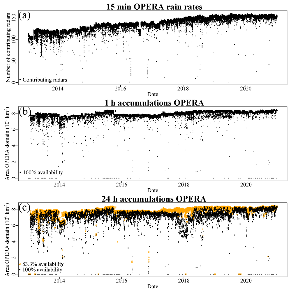
Figure 1OPERA radar data availability as a function of time over the period 2013–2020. (a) Number of contributing radars to the OPERA composite of rain rates in case data are available for at least part of the OPERA domain. Coverage of OPERA radar datasets as a function of time for the (b) 1 and (c) 24 h precipitation accumulations. For panels (b) and (c), time intervals without data are also plotted (as 0).
For each radar grid cell (pixel) and clock hour (i.e., every hour on the hour), 1 h precipitation accumulations are computed from the rain rates in case of full availability; otherwise, the grid cells contain the ODIM “nodata” value, which is “used to denote areas void of data (never radiated)” (Michelson et al., 2019). So, 1 h accumulations are only derived if all 15 min OPERA rain rates are not equal to the nodata value and “undetect” values from the OPERA rain rates, “used to denote areas below the measurement detection threshold (radiated but nothing detected)” (Michelson et al., 2019), are set to 0 mm. These 1 h precipitation accumulations are used to compute 24 h accumulations every clock hour as well as annual accumulations. For each radar grid cell, a minimum data availability of the underlying 1 h accumulations of 83.3 % is required (i.e., at least 20 of 24 h or ∼ 304.2 of 365 d). Grid cells with overly low availability are set to the OPERA nodata value. The availability of 1 and 24 h precipitation accumulations is generally high (Fig. 1b–c). For the large majority of the OPERA domain, the availability of 1 h precipitation accumulations is at least 95 % over the period 2013–2020 (Fig. 2a). The distance to the nearest radar displays quite some variability but is generally shorter than 175 km (Fig. 2c). The median and mean distances to the nearest radar are 110 and 133 km, respectively. Some countries do have radars, but these do not contribute to the OPERA composite yet (e.g., Austria and Italy). All derived radar datasets are kept in ODIM-HDF5 format on the default OPERA grid of 2 km resolution.
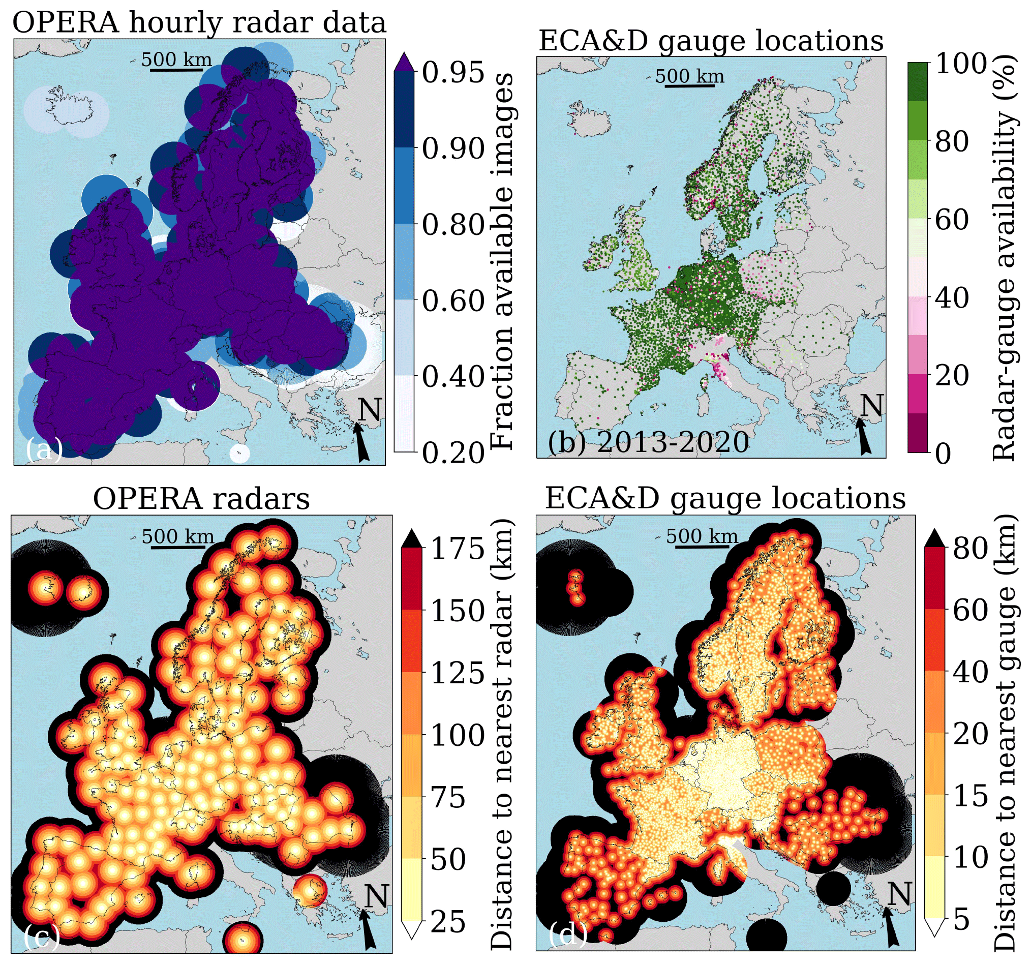
Figure 2(a) Map of the OPERA domain with the fraction of available radar composites over the period 2013–2020. (b) Map with combined radar–gauge availability over the period 2013–2020. (c) Map of the distance to the nearest radar per grid cell assuming full availability of radar data (note that some of the radars only contributed part of the period). (d) Map of the distance to the nearest rain gauge per grid cell assuming full availability of radar and gauge data. This shows the best possible result. In reality, the average minimum distance will be longer because sometimes gauge data are missing. Maps made with Natural Earth. Free vector and raster map data © https://naturalearthdata.com (last access: 23 March 2023).
2.2 European Climate Assessment and Dataset and E-OBS rain gauge data
Daily precipitation series were obtained from the European Climate Assessment and Dataset (ECA&D, https://www.ecad.eu, last access: 23 March 2023) project (Klein Tank et al., 2002; Klok and Klein Tank, 2008). In total, ∼ 7700 rain gauges from 29 different countries and 37 different data providers, including non-downloadable series (i.e., included in ECA&D for production of derived data but only accessible through the data-owning NMHSs), are covered by OPERA radars during (part of) the 2013–2020 period. Combined radar–gauge data availability is at least 90 % for most regions (Fig. 2b). This availability is the percentage of daily intervals in the 8-year period at each gauge location, where the gauge and corresponding radar accumulations are both available. Figure 2d displays the distance to the nearest gauge for the OPERA domain if all ∼ 7700 gauges are available. The large variability in space of the underlying rain gauge network density is obvious. The median and mean distances to the nearest rain gauge are 42 and 92 km, respectively. These relatively long distances are mainly caused by areas above the land surface with low rain gauge network densities and above the sea. The ECA&D rain gauge dataset will be used to evaluate the various radar precipitation datasets and will be merged with 1 h radar accumulations.
The rain gauge data have undergone quality control by the ECA&D team (Project team ECA&D and Royal Netherlands Meteorological Institute KNMI, 2021) and often by NMHSs. Given the latency in gauge data provided to ECA&D for some networks and to prevent spatial differences in the quality of merged radar–gauge QPE, only data up to and including 2020 are used. At the time of data production (mid-June 2022), it was found for some countries that the density of gauge networks from which data were available is relatively sparse (Bosnia and Herzegovina, Croatia, Denmark, Hungary, Iceland, Lithuania, Portugal, Romania, Slovakia, Spain, Switzerland) and no data are available (e.g., Bulgaria, Greece, Kosovo, North Macedonia) or are not complete for the entire period (e.g., for Romania it ends on 31 September 2020, for Serbia it ends on 31 December 2017, it is only a few years for Montenegro, and time series from most stations in the United Kingdom end on 31 December 2019).
The daily measurement interval of gauges is often not exactly known to ECA&D. For instance, the metadata for some networks are imprecise as aggregation intervals ending at 06:00, 07:00 or 08:00 UTC are lumped together. Sometimes, additional information on the measurement interval end time from the respective NMHS was available and selected. In order to determine the exact measurement interval for other gauge networks, gauge accumulations are compared to OPERA 24 h accumulations by testing different measurement interval end times. For each network, distributions of Pearson correlation coefficients for all gauge locations are evaluated for each interval end time using ridgeline plots. The measurement interval end time with the highest correlations is selected for that given network. The end times of the observations display a large variability across Europe at 00:00 UTC (9 networks), 06:00 UTC (16 networks), 06:00 UTC in summer and 07:00 UTC in winter (1 network), 07:00 UTC (1 network), 08:00 UTC (3 networks), 09:00 UTC (2 networks), 18:00 UTC (3 networks) and 21:00 UTC (1 network) to 22:00 UTC in summer and 23:00 UTC in winter (1 network).
A pan-European dataset, E-OBS version 25.0e (https://surfobs.climate.copernicus.eu/dataaccess, last access: 23 March 2023), of gridded, daily and interpolated ECA&D gauge accumulations (Cornes et al., 2018) is used to compute annual precipitation accumulations. These will be used for comparison with EURADCLIM accumulations.
2.3 Satellite cloud-type product
Information on the occurrence and type of clouds was obtained from the Spinning Enhanced Visible and Infrared Imager (SEVIRI) on board the geostationary Meteosat Second-Generation (MSG) satellites operated by the European Organisation for the Exploitation of Meteorological Satellites (EUMETSAT). The CLoud property dAtAset using SEVIRI edition 2 (CLAAS-2) was used, produced by EUMETSAT's Satellite Application Facility on Climate Monitoring (CM SAF). CLAAS-2 (Finkensieper et al., 2016; Benas et al., 2017) is a climate data record of cloud properties derived from SEVIRI measurements and extending from 2004 to the present. The CLAAS-2 cloud-type product was derived with the MSGv2012 software package developed by the SAF on nowcasting and very-short-range forecasting (NWC SAF). Further details on the retrieval algorithm can be found in Derrien and Le Gléau (2005) and NWC SAF (2013). The temporal resolution of CLAAS-2 is 15 min. Its spatial resolution is 3 km × 3 km at the subsatellite point and around 4 km × 7 km in the center of the OPERA domain (∼52∘ N). The cloud type was converted from the CLAAS-2/SEVIRI grid to the native OPERA radar grid of 2 km by 2 km using nearest-neighbor resampling. This dataset is available day and night and is used to remove non-meteorological echoes from the OPERA radar data. Over the period 2013–2020, 99.7 % of the 15 min intervals have valid data.
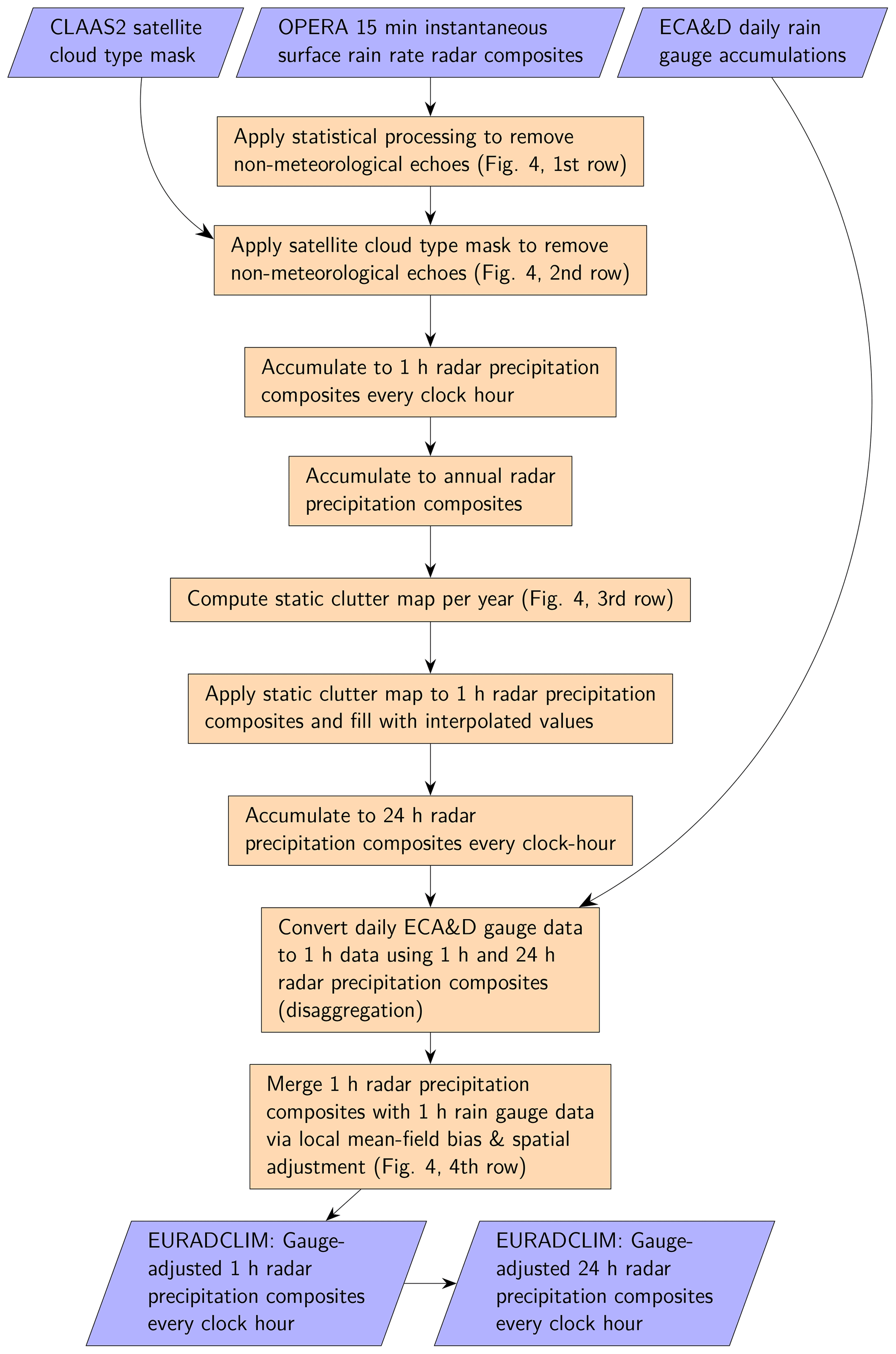
The flowchart in Fig. 3 provides an overview of the input datasets, the applied processing and the output dataset EURADCLIM. Three algorithms are applied to further remove non-meteorological echoes from the OPERA radar data. Finally, the radar data are merged with the ECA&D rain gauge data.
3.1 Gabella clutter filter
The function clutter.gabella from the open-source Python library for weather radar data processing wradlib version 1.9.0 (Heistermann et al., 2013; Mühlbauer et al., 2020) is employed to classify non-meteorological echoes. This Gabella filter is a two-part algorithm (Gabella and Notarpietro, 2002; Wradlib, 2021), which uses as input the radar reflectivity factors. For this, rain rates are converted to radar reflectivity factors employing Zh=200R1.6 (beforehand undetect and nodata values are set to 0 mm h−1). Then the Gabella filter is used to classify grid cells using the Cartesian radar reflectivity factor data. In the first part of the filter, strong spatial gradients are identified by checking for each grid cell how many cells surrounding it in a square lattice of 5×5 cells are less than 6 dBZh lower than the central cell. When this number of cells is lower than 6, the central cell is identified as clutter. In the second part of the filter, the ratio between the area and circumference for contiguous echo regions is computed, where these consist of cells with a value above 0 dBZh. When the absolute value of this ratio is lower than 1.3, the central cell is identified as clutter. Next, the original surface rain rates are set to 0 mm h−1 in case one or two of the parts of the Gabella filter identify clutter. Central cells that have nodata values in the original rain rates are unaffected by the Gabella filter, and undetect values are kept in case of no clutter. A successful example of applying the Gabella clutter filter for the Netherlands and surroundings is provided in Fig. 4a–b.
3.2 Satellite cloud-type mask clutter filter
A satellite cloud-type mask is employed to classify remaining non-meteorological echoes. Localization errors (e.g., advection, timing differences between radar and satellite, parallax) are taken into account by considering all grid cells in a square lattice of 7×7 cells containing the central cell for which the classification is performed. The rain rate for this central cell is set to 0 mm h−1 when all cells in the square lattice are either classified as cloud-free or as containing semitransparent clouds (which are assumed to be non-raining). Concretely, these cases correspond to the following MSGv2012 cloud-type categories: cloud-free land, cloud-free sea, land contaminated by snow, sea contaminated by snow/ice, high, semitransparent thin clouds, high, semitransparent meanly thick clouds, and high, semitransparent thick clouds. In case satellite data are not available for a given pixel (category “non-processed containing no data or corrupted data” or no file/image available), that pixel is not used as a neighboring pixel, and the radar pixel directly beneath it will not be labeled as clutter. Figure 4c–e illustrate the working of this algorithm by providing a 15 min radar rain rate, before and after applying the satellite cloud-type mask, which is also displayed. Because the satellite images are referenced to with the start time of observation and the radar composites are referenced to with the end time of observation, a satellite image of, for example, 12:00 UTC is combined with the radar composite of 12:15 UTC.
3.3 Static clutter filter
The 15 min radar rain rates are accumulated to 1 h and these 1 h accumulations to annual precipitation accumulations. The function clutter.histo_cut from the open-source Python library for weather radar data processing wradlib version 1.9.0 (Heistermann et al., 2013; Mühlbauer et al., 2020; Wradlib, 2022) is employed to classify non-meteorological echoes in the annual precipitation accumulation. First, a histogram of 50 classes is computed from the annual precipitation from a given year using all grid cells. Next, the class with the largest frequency is determined. An iterative procedure detects those classes with a frequency below 5 % of the frequency of the class with the largest frequency (the hard-coded default value is 1 %). The procedure stops when the changes in the maximum annual rainfall from the remaining classes become (smaller than) 1 mm compared to the previous iteration. The grid cells corresponding to the detected classes become the static clutter mask. For each year a separate static clutter mask is obtained. This algorithm identifies areas with static clutter and may also detect areas affected by beam blockage. Next, inverse-distance-weighted interpolated values are computed for the identified grid cells (inverse distance-weighting power of 2; maximum of four neighbors). This value replaces the original value only in case it is lower than the original value. The original nodata values are kept in the output dataset. The interpolation is performed on the 1 h precipitation accumulations. From the cleaned 1 h accumulations, which are used for merging with rain gauge accumulations, 24 h accumulations for every clock hour are derived. Figure 4f–h show an example of annual precipitation accumulations, the derived annual precipitation accumulations after applying the static clutter mask including interpolation on the underlying 1 h radar precipitation composites and the corresponding static clutter mask. The mask seems to correspond mostly to areas with high annual precipitation. In theory, the interpolation could decrease precipitation estimates for areas with beam blockage. Areas with beam blockage are not abundant, though. Also note that a beam-blockage correction has already been applied by OPERA.
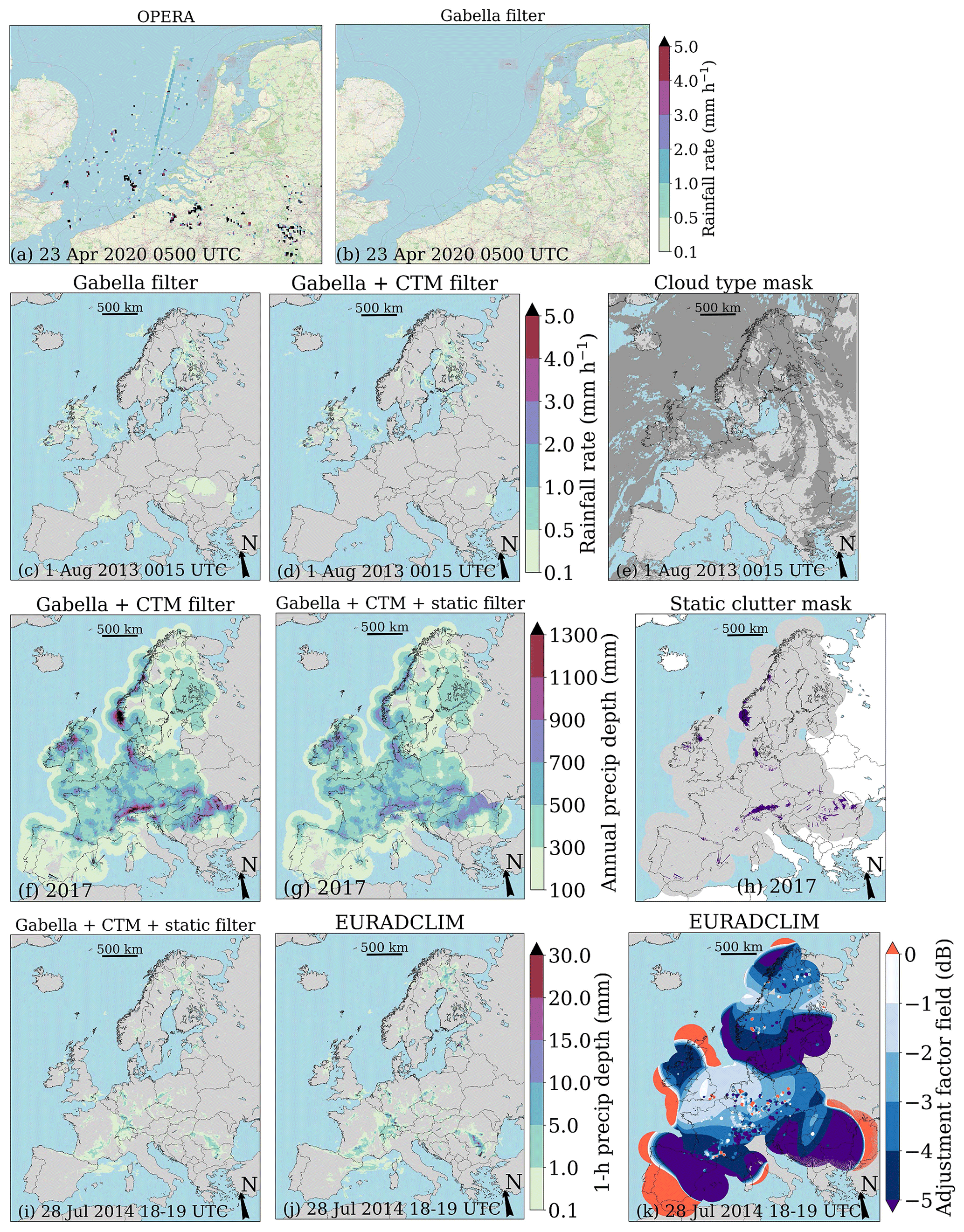
Figure 4Illustration of the application of all three clutter-removal steps and the rain gauge adjustment, i.e., of all processing steps in EURADCLIM. (a)–(b) Application of the Gabella clutter filter (map data © OpenStreetMap contributors 2022. Distributed under the Open Data Commons Open Database License (ODbL) v1.0) and of (c)–(e) the cloud-type mask to remove non-meteorological echoes from a 15 min OPERA composite of rain rates. For the cloud-type mask, the grey areas indicate where the cloud type does not belong to the seven categories listed in Sect. 3.2 and for which the radar rain rates were thus left untouched. (f)–(h) Illustration of the application of the static clutter mask, derived from the annual precipitation map, to 1 h radar precipitation composites, which are accumulated to an annual precipitation map. (i)–(k) Application of the radar–gauge merging algorithm going from unadjusted to adjusted 1 h rainfall accumulations employing the 1 h adjustment factor field. (c)–(k) Maps made with Natural Earth. Free vector and raster map data © https://naturalearthdata.com (last access: 23 March 2023).
3.4 Merging radar with ECA&D rain gauge data
The starting point of the merging algorithm is that radar and rain gauge data are used from the same 1 h interval, instead of computing adjustment factor fields based on preceding time intervals, such as in Park et al. (2019). Since the measurement interval of daily rain gauge accumulations varies across Europe, a daily adjustment factor field would not be entirely representative, and since the aim is to derive 1 h adjusted radar precipitation accumulations, ideally, 1 h adjustment factor fields would be computed. To achieve this, the daily gauge accumulations are disaggregated to 1 h accumulations employing the 1 and 24 h radar accumulations from the previous processing step. The end times of the observations, as determined in Sect. 2.2, are taken into account in the disaggregation. It is assumed that the gauges observed precipitation only during the intervals for which radar data were available. So, in the case of missing radar data, at most 4 h per 24 h interval, the daily gauge precipitation is only distributed over the remaining (at least 20) hours. The threshold of 4 h comes from the minimum required availability of 83.3 % to aggregate 1 to 24 h radar accumulations. If this requirement is not met for a given radar grid cell and 24 h interval, the nodata value is assigned to the radar grid cell. Hence, if more than 4 h of radar data at the location of a rain gauge is missing per 24 h, the disaggregation to 1 h gauge values cannot be performed. The merging of 1 h disaggregated rain gauge data and radar data is simply performed with all available radar–gauge pairs. If no radar–gauge pairs are available at all, due to either missing radar (i.e., only nodata values at gauge locations) or rain gauge data, the merging is not performed, and EURADCLIM will be a copy of the unadjusted radar dataset. Next, to decrease the computation time of the radar–gauge merging, only 1 h radar–gauge pairs for which gauge precipitation exceeds 0.25 mm are used for merging. This is expected to have a limited effect on the quality of the merged dataset.
The radar–gauge merging algorithm is based on Barnes' objective analysis (Barnes, 1964) but has been extended to make it robust in the case of sparse gauge network densities for short durations (1 h), when spatial precipitation variability is often large. A spatial adjustment factor field Fc is computed from the distance-weighted interpolation of the raw radar precipitation accumulations (Sw,r) and the interpolation of the corresponding gauge precipitation accumulations (Sw,g), implying that it is computed for each radar grid cell, which has the position (x,y):
with T a threshold value of 0.25 mm. Sw,X, with X an indicator being g (gauge) or r (radar), is defined as
which is computed over NP radar–gauge pairs. Rr,n and Rg,n are the precipitation accumulations at the gauge location n for radar and gauge, respectively. In case the value of Sw,X is below T, it is set equal to T. This is done to prevent outliers in the gauge-adjusted radar precipitation accumulations. The weighting function wn depends on the distance of a grid cell to the gauge location:
where Gw(n,rd) is a Gaussian function:
and (xn,yn) is the position of gauge n. Equation (3) employs two Gaussian functions, each with its own characteristic distance rd, for which the influence of a gauge is reduced to 0. The shorter range, rs, results in a local adjustment in the neighborhood of gauges. The value of rs is taken as the range of an isotropic spherical variogram model, which has been expressed as a function of the day of year (DOY) and duration (1–24 h) using a 30-year rain gauge dataset from the Netherlands from the period 1979–2009 (Van de Beek et al., 2012). When distances from a grid cell to gauges are longer than rs, this short-range component does not contribute to the adjustment. The longer range, rl, set at 500 km, is used to also adjust when gauge network density is sparse and the nearest gauges are far away (e.g., over the sea). The value of v controls the contribution of this long-range component with respect to the short-range component. Apart from the actual adjustment in which all selected gauges are used, leave-one-out statistics (LOOS) are also provided. These statistics are computed based on adjusted radar precipitation accumulations computed for a given gauge location without using that particular gauge in the adjustment. This is repeated for each gauge location, thus allowing for an independent verification of the gauge-adjusted radar dataset.
The algorithm can also run two adjustments consecutively with different settings while still providing LOOS. Here, first an adjustment is performed with v=100 000, implying a local mean-field bias adjustment taking into account all gauges within a radius of 500 km. The short-range component does not play a role then. This helps to remove systematic underestimations as much as possible in regions with low-gauge network densities. Tests indicated that underestimations could not be effectively removed when the short-range component also contributed. Next, v is set to 0, implying that only a local spatial adjustment is performed on top of the already mean-field bias-adjusted precipitation estimates. The adjustment factor fields from both adjustments are combined into one 1 h spatial adjustment factor field. The 1 h radar precipitation composite is divided by this adjustment factor field to obtain the 1 h adjusted radar precipitation composite (EURADCLIM). Figure 4i–k illustrate the adjustment by showing an unadjusted radar composite, the adjusted radar composite and the adjustment factor field. The effect of the long- and short-range components is visible in the adjustment factor field, where the large-scale patterns belong to the long-range component (v=100 000) and the local patterns (dots) show the influence of the short-range component (v=0) on top of the long-range component.
3.5 Evaluation
The radar precipitation accumulations are evaluated against rain gauge accumulations by means of scatter density plots, maps with station-based spatial verification, comparison of annual precipitation maps to those based on gridded rain gauge data (E-OBS) and statistical metrics. In addition, maps of the mean hourly precipitation and the relative frequency of exceeding a threshold value of 1 h precipitation are compared between different processing steps. Statistical metrics used for evaluation are the relative bias of radar precipitation accumulations compared to the corresponding gauge precipitation accumulations, the residual standard deviation divided by the mean gauge precipitation accumulation (i.e., the coefficient of variation, CV), the Pearson correlation coefficient (ρ) and the mean absolute error (MAE). Here, a residual is defined as the radar precipitation accumulation minus the gauge precipitation accumulation. Results are provided for all radar–gauge pairs as well as for the subset where the gauge exceeds thresholds of 1.0, 10.0 and 20.0 mm d−1. Note that representativeness errors can be significant when comparing radar and gauge accumulations (Kitchen and Blackall, 1992), especially for shorter durations, such as 1 h, and in the case of larger differences in measurement volumes. The grid cell size of 4 km2 is relatively large. Radars measure aloft, and rain gauges measure at the Earth's surface, but only over a small area. Hence, differences between radar and gauge accumulations can be partly attributed to representativeness errors.
The radar precipitation datasets are assessed by first systematically evaluating the influence of the clutter-removal algorithms on QPE, followed by an evaluation of the performance of the EURADCLIM precipitation estimates. EURADCLIM's pan-European precipitation climatologies are shown, and EURADCLIM's limitations are discussed. Finally, extreme precipitation events derived from EURADCLIM are presented.
4.1 Evaluation of clutter-removal algorithms
Maps of mean hourly precipitation over the period 2013–2020 (Fig. 5a–b) show that the Gabella clutter filter removes and reduces many non-meteorological echoes, e.g., sea clutter at the North Sea, rings around Denmark, a radial pattern around Estonia and spokes caused by interference over Slovakia. Also, areas belonging to the highest precipitation class become smaller in Romania and southern France. Additional reductions are less pronounced when the cloud-type mask is applied (Fig. 5b–c). A clear reduction in interferences in eastern Spain stands out, and areas falling into higher precipitation classes become smaller in Romania. The static clutter mask is effective in (strongly) reducing many of the remaining non-meteorological echoes (Fig. 5c–d). When using a shorter color scale (not shown), it becomes visible that for some areas values may still be too high, and then the area in Europe known for the highest annual precipitation, the coastal area of Norway, also shows a strong reduction, which may point to unwarranted classification of non-meteorological echoes. This can be seen more clearly in Fig. A1c.

Figure 5Comparison between 1 h precipitation accumulations from four datasets to study the effect of non-meteorological echo-removal algorithms over the period 2013–2020. Results are only shown for grid cells with a minimum availability of 83.3 %. (a)–(d) Maps of mean hourly precipitation and (e)–(l) maps of the relative frequency of exceedance of 0.1 and 5 mm in an hour. These are obtained by dividing by the number of available values for each individual radar grid cell (i.e., not equal to “nodata” or not missing). This implies that periods with missing radar data are not taken into account, and the number of intervals that is used will vary in space. Maps made with Natural Earth. Free vector and raster map data © https://naturalearthdata.com (last access: 23 March 2023).
From the maps of the relative frequency of 1 h precipitation exceeding 0.1 mm (Fig. 5e–f) and 5 mm (Fig. 5i–j), it can be concluded that the Gabella filter successfully removes non-meteorological echoes, especially sea clutter and suspicious noisy areas above land. The circles and radial patterns found for mean precipitation are not apparent, indicating that these do not occur frequently. For the 0.1 mm threshold, application of the cloud-type mask clearly reduces the impact of interferences above Spain, and some areas belonging to the highest precipitation classes become smaller or disappear, especially in eastern Europe and south of the French Mediterranean coast. It is apparent that larger areas above France and Germany now belong to a lower-frequency class, which could point to unwarranted classification of non-meteorological echoes. The cloud-type mask hardly adds value in removing non-meteorological echoes for the 5 mm threshold, apart from reducing the frequency of the impact of interferences (Fig. 5j–k). The static clutter mask successfully removes non-meteorological echoes for the 0.1 mm threshold (Fig. 5g–h) in eastern Europe, and for the 5 mm threshold (Fig. 5k–l), the frequency of the remaining interferences is successfully decreased over all of Europe. The fraction in mean rainfall and the fraction in relative frequencies of these datasets, which have undergone additional clutter removal, with respect to the OPERA dataset are presented in Appendix A.
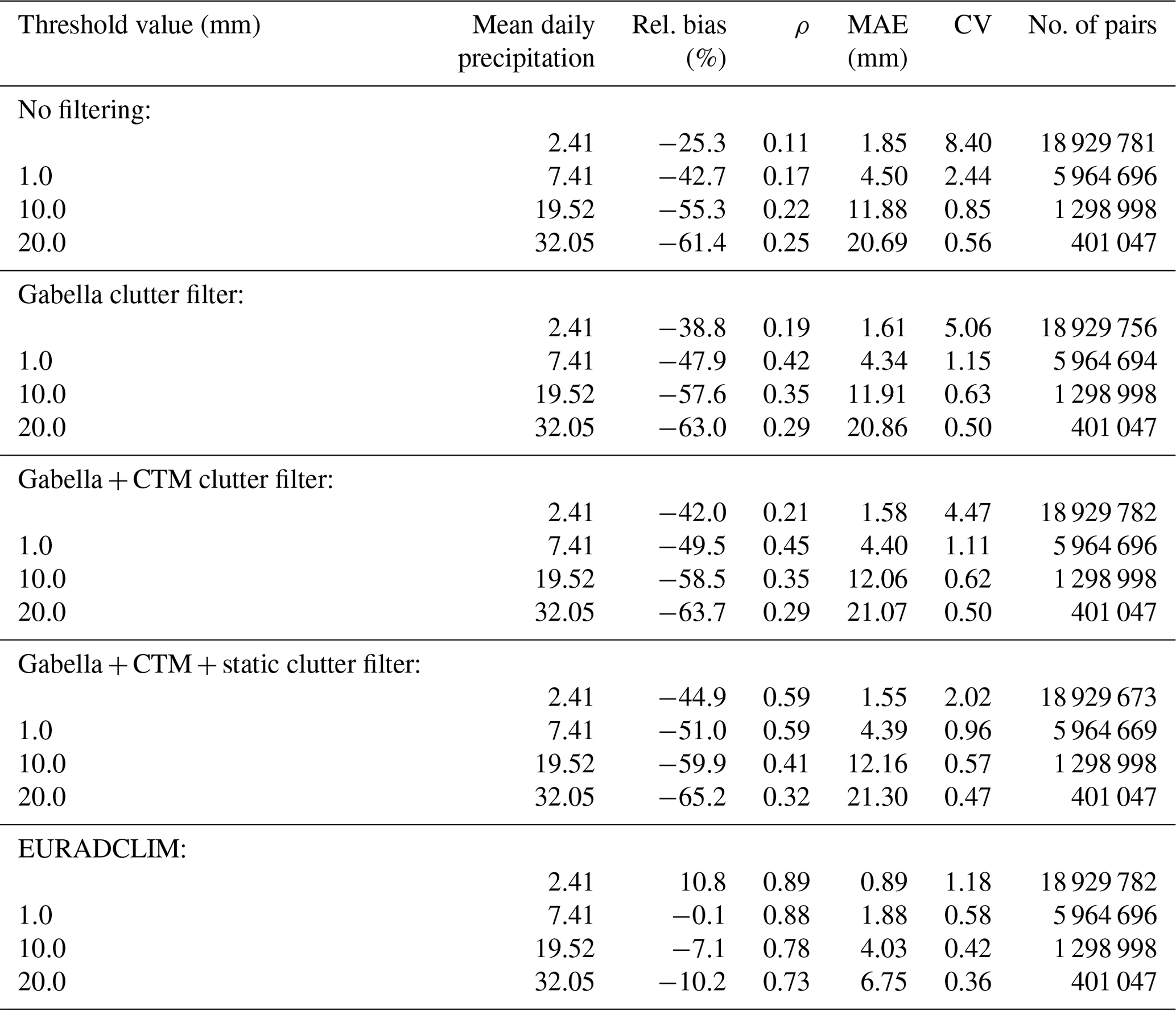
The conclusion is that the algorithms remove many and also severe non-meteorological echoes. To evaluate the unwarranted removal of precipitation echoes, daily radar accumulations are compared to daily gauge accumulations in Table 1. This independent evaluation for different threshold values shows that differences in the value of MAE between the four datasets are small, the value of CV usually decreases, and the value of ρ usually increases after each additional processing step. The strongest improvement is found for the Gabella clutter filter and the static clutter filter. The relative bias in the mean daily precipitation becomes much more negative though. The non-meteorological echoes may have compensated for the large underestimation that is typical for mid- to high-latitude radar-only precipitation estimation (Overeem et al., 2009b). Because of the general improvement for other statistical metrics, it is concluded that the clutter-removal algorithms are effective and remove a few precipitation echoes. In conclusion, the radar dataset that will be used for merging with rain gauge data has improved considerably over the dataset where no additional filtering is applied in terms of ρ and CV.
As a final check of the effectiveness of the clutter filter, daily radar accumulations are selected when the daily gauge accumulation is 0 mm. This results in average daily accumulations of 0.5 mm when no filtering is applied, and this decreases to 0.3 mm for the Gabella filter and to 0.2 mm when the cloud-type mask is also applied. This confirms the effectiveness of the algorithms in further removing non-meteorological echoes. It remains 0.2 mm, though, when the static clutter filter is also applied. This is likely a result of the static clutter mask being only applied to a small part of the OPERA domain (see, e.g., Fig. 4h), which contains a small minority of the rain gauges. As a consequence, positive effects are small when compared to rain gauges from the entire OPERA domain. Moreover, in contrast to the other clutter-filtering algorithms, values are not removed but are interpolated from the surrounding values. Hence, no clear improvement at the location of the gauges is found for the static clutter mask.
Table 1Evaluation of radar daily precipitation accumulations against the ECA&D rain gauge network over the period 2013–2020 at their default measurement interval for all radar–gauge pairs and for those above a threshold value. The mean daily precipitation and the threshold value are based on the gauge data. Relative bias, Pearson correlation coefficient, mean absolute error, coefficient of variation and number of radar–gauge pairs are provided, respectively.
4.2 Evaluation of EURADCLIM
In Table 1, a dependent verification of daily radar precipitation accumulations against rain gauges is performed to quantify the influence of the adjustment employing gauge data (i.e., with respect to the “Gabella + CTM + static filter” dataset). Results are presented for all values and for those where gauges exceed specific thresholds. Note that all selected values are used to compute the statistical metrics. A number of conclusions can be drawn from Table 1. (1) The severe average underestimation of precipitation of ∼ 45 % turns into an overestimation of ∼ 11 % for EURADCLIM. (2) For daily gauge precipitation above 1 mm the relative bias is near zero. (3) The large underestimation for very-heavy precipitation days (over 20 mm d−1) is reduced from ∼65 % to about ∼10 %. (4) The value for the correlation coefficient strongly increases from 0.59 to 0.89 based on all precipitation events. (5) The values for CV strongly decrease with a factor between 1.3 and 1.7. (6) The values for MAE decrease to values that are between 1.7 and 3.2 times smaller. The scatter density plots provide a more complete overview of the improvement and show the much better alignment along the 1:1 line compared to the unadjusted dataset for daily gauge precipitation above 1 mm (Fig. 6a–b). The quality of daily precipitation accumulations is higher in summer (June, July, August; Fig. 6d) than in winter (December, January, February; Fig. 6c). Although differences in the values of statistical metrics are relatively small, the spread in the scatter density plot for summer is clearly lower than in winter. The (near-)zero precipitation values for a wide range of rain gauge values are apparent; 54 % of all data points for which the daily gauge accumulation is above 20 mm and the corresponding EURADCLIM radar accumulation is below 1 mm (Fig. 6b) are located in Italy and are likely related to beam blockage or overshooting.
For hourly precipitation, both an independent verification via leave-one-out statistics and a dependent verification are performed. The scatter density plots show the radar–gauge pairs for 1 h gauge precipitation larger than 0.25 mm (Fig. 6e–g). The remaining underestimation becomes small, and the value for the coefficient of determination (ρ2) increases with respect to the unadjusted radar dataset, especially for the dependent verification. For EURADCLIM, the value for CV increases for the independent verification. The second-lowest count class becomes rather wide above the 1:1 line. For the dependent verification the scatter density plot is much better aligned to the 1:1 line, and the value for CV becomes much lower compared to the unadjusted dataset. The conclusion is that the quality of the EURADCLIM dataset is good and much better than the dataset that has undergone the clutter filtering but no gauge adjustment. Note that the verification via LOOS is not entirely independent, because the 1 and 24 h radar accumulations have been employed to disaggregate the daily gauge accumulations to hourly accumulations.
Next, a spatial verification per rain gauge location is performed for the radar dataset before gauge adjustment and for EURADCLIM, again for an independent verification (LOOS) and a dependent verification (Fig. 7). The quality of the radar composite for the unadjusted radar dataset displays quite some variability, and there seems to be some connection with areas further away from the nearest radar (Fig. 2c). Also, different environmental conditions, e.g., beam blockage due to mountainous terrain, can play a role. The values for ρ, CV and relative bias in the mean strongly improve for the EURADCLIM dataset (dependent verification; Fig. 7c, f, i) with respect to the unadjusted radar dataset. In addition, the spatial variability in performance becomes much smaller. However, for the independent verification for regions with low gauge network densities, the value for ρ sometimes decreases, the value for CV often increases, the underestimation becomes either less severe or turns into a large overestimation (Fig. 7b, e, h) with respect to the unadjusted radar dataset. Note that the dependent verification shows the actual performance of EURADCLIM at those locations and that the independent verification is meant to give an impression of the quality between those locations. In reality, results are expected to be better for EURADCLIM than found for this independent verification, because the distance to the nearest gauge will be much shorter. For the LOOS results, the gauge adjustment has been rerun for each gauge location while using all available radar–gauge pairs except the one at the considered gauge location, whereas for EURADCLIM, all available radar–gauge pairs are used.
Finally, for some gauge locations, large differences are found. For instance, for two nearby stations in Poland, a large overestimation and a large underestimation are found. Also, the values for CV are high. This may point to erroneous rain gauge data. For other regions, radar beam blockage could play a role.
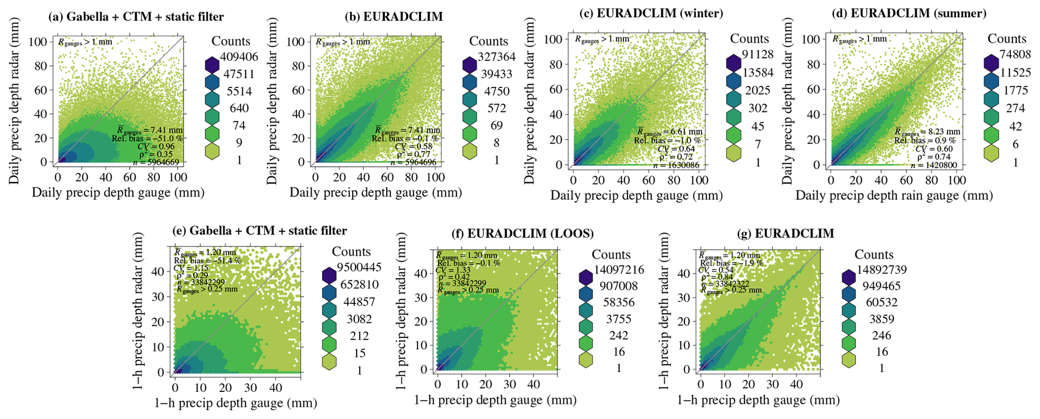
Figure 6Scatter density plots of (a)–(d) daily and (e)–(g) 1 h radar precipitation accumulations against rain gauges over the period 2013–2020. For daily accumulations the gauge accumulations at their default measurement interval are employed, whereas for 1 h accumulations the disaggregated clock-hourly gauge precipitation accumulations are employed. Results are shown for the unadjusted dataset that has undergone all clutter-filtering steps and for the gauge-adjusted EURADCLIM dataset. For EURADCLIM, independent verification is done via leave-one-out statistics (LOOS), when indicated. Otherwise, the verification is dependent.

Figure 7Spatial verification of 1 h precipitation accumulations against the disaggregated clock-hourly gauge precipitation accumulations over the period 2013–2020. (a, d, g) For the unadjusted radar dataset that has undergone all clutter-filtering steps. Results from the gauge-adjusted EURADCLIM dataset are shown for (b, e, h) an independent verification employing LOOS and for (c, f, i) a dependent verification. Maps made with Natural Earth. Free vector and raster map data © https://naturalearthdata.com (last access: 23 March 2023).
4.3 EURADCLIM radar precipitation climatologies and their limitations
Despite the efforts by NMHSs and OPERA to remove non-meteorological echoes and the three additional clutter-removal algorithms employed to derive EURADCLIM, non-meteorological echoes can still be persistent for some areas (Fig. 5h). Two cases with strong artifacts are shown in Fig. 8 for the original OPERA surface rain rates. For the first case, the entire radar domain of a Spanish radar has very high rates, which seems to be caused by a constant signal source that lasted the first 7 h of 29 April 2018 (Fig. 8a). Since this occurs over an entire radar domain, the algorithms can only partly remove and reduce these echoes caused by failures of radar processing (unless entirely cloud-free or only semi-transparent clouds). This is much reduced by the gauge adjustment, although 24 h precipitation accumulations of more than 50 mm are still found in EURADCLIM (Fig. 8b). For the second case (Fig. 8c) with strong artifacts from a French radar, the 1 h precipitation accumulations are substantially reduced by the EURADCLIM algorithms (Fig. 8d). Again, this reduction is primarily caused by the gauge adjustment. Still, Fig. 8b, d indicate that EURADCLIM sometimes contains substantial artifacts.
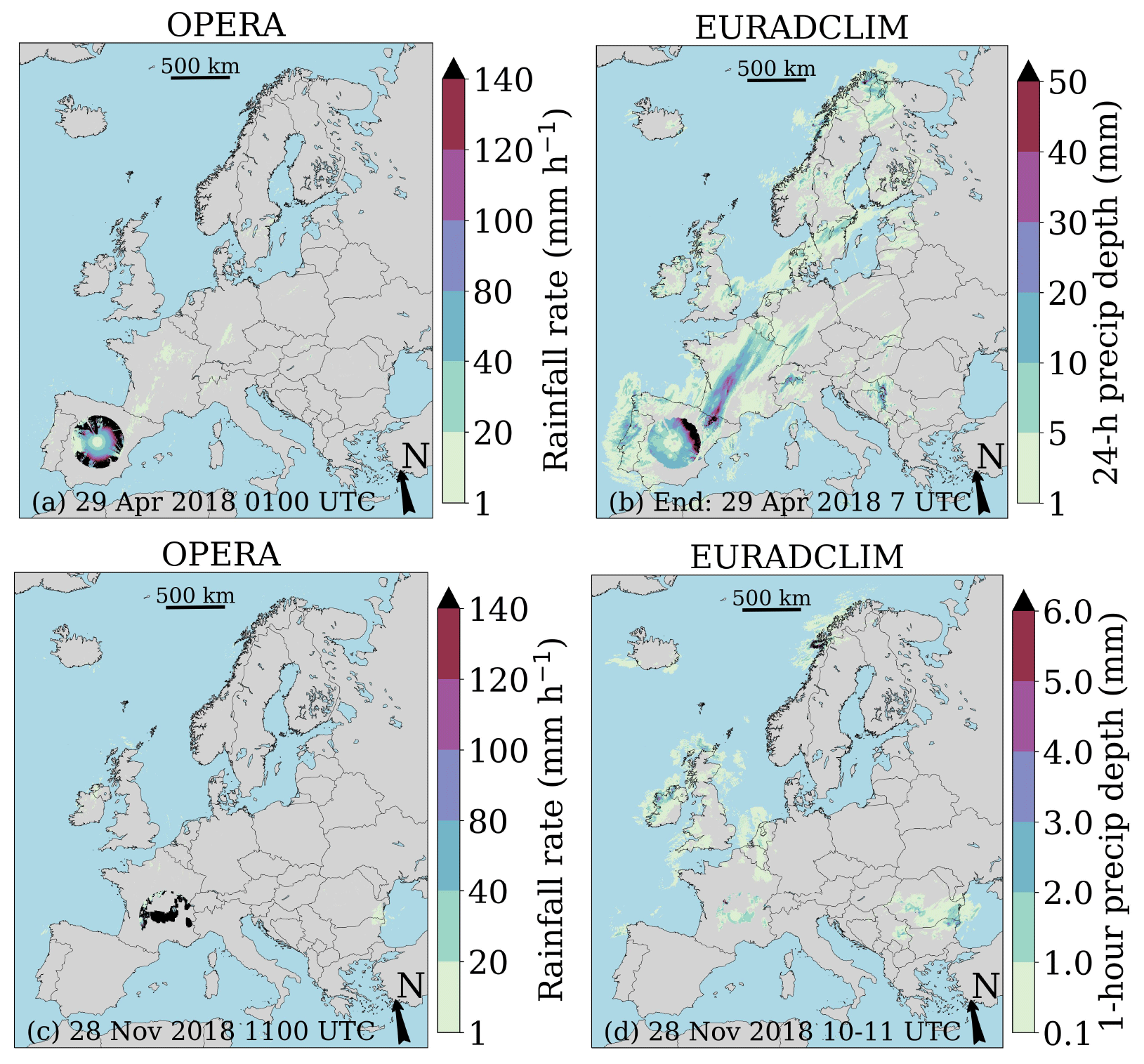
Figure 8Illustration of the remaining non-meteorological echoes in radar data for the original instantaneous OPERA rain rates and the corresponding 24 h or 1 h precipitation accumulations from EURADCLIM. (a)–(b) Extreme values in central Spain on 29 April 2018 01:00 UTC (rain rate) and from 28 April 2018 07:00 UTC to 29 April 2018 07:00 UTC (24 h precipitation accumulation). The gauge adjustment helps to lower the accumulations in EURADCLIM. (c–d) An extreme case with more than 500 mm h−1 over large parts of a French radar domain on 28 November 2018 for 11:00 UTC. Clutter-removal algorithms hardly help, but the gauge adjustment substantially reduces the 1 h precipitation accumulations from EURADCLIM from 10:00 to 11:00 UTC. Maps made with Natural Earth. Free vector and raster map data © https://naturalearthdata.com (last access: 23 March 2023).
Now that the quality of EURADCLIM has been quantified, precipitation climatologies are derived to show its potential (Fig. 9). A map of mean hourly precipitation over the period 2013–2020 is shown in Fig. 9a. There are still some signatures of beam blockage (e.g., Austria, Italy and northwestern Spain in Fig. 9a), probably caused by obstacles near radar sites, and of non-meteorological echoes, such as interferences (e.g., Bosnia and Herzegovina and eastern Spain in Fig. 9a, f, g). The highest precipitation values are found in the coastal areas of Norway and in some mountainous areas (e.g., the Alps, Bosnia and Herzegovina, Croatia, Ireland, Norway, Scotland and Wales). The seasonality of mean hourly precipitation is visualized in Fig. 9b–e. In western Europe, precipitation is highest in fall and winter. The Mediterranean areas are typically dry in winter and summer and relatively wet in spring and fall. The high seasonal precipitation in the Alps in summer is apparent. Relative frequencies exceeding 0.1 mm are displayed in Fig. 9f, revealing that 1 h precipitation is most frequent in Denmark, Ireland, large parts of the United Kingdom, parts of Norway and a patchy band from France to Switzerland and Germany and parts of eastern Europe. The southern part of Spain has the lowest frequency of 1 h precipitation exceeding 0.1 mm. The relative frequency exceeding 5 mm (Fig. 9g) shows that more extreme precipitation occurs most often in parts of southern Europe and parts of Ireland and the United Kingdom. It is difficult to tell to what extent non-meteorological echoes play a role here. For instance, some of the localized areas with high frequencies exceeding 5 mm may be related to obstacles near radar sites. This becomes even more apparent for downpours of more than 25 mm in 1 h (Fig. 9h), where large areas are found with at least 13 occurrences in 8 years, sometimes present over a large part of a radar domain. These large values at the edge of radar coverage are suspicious, especially when no nearby rain gauges are available, such as east of the island of Corsica (France). When comparing the mean daily precipitation and relative frequencies exceeding 0.1 and 5 mm to those from the unadjusted radar data in Fig. 5, it is clear that these strongly increase after the gauge adjustment. This can also lead to non-meteorological echoes becoming more pronounced (e.g., interferences in eastern Spain in Fig. 9f compared to Fig. 5h).
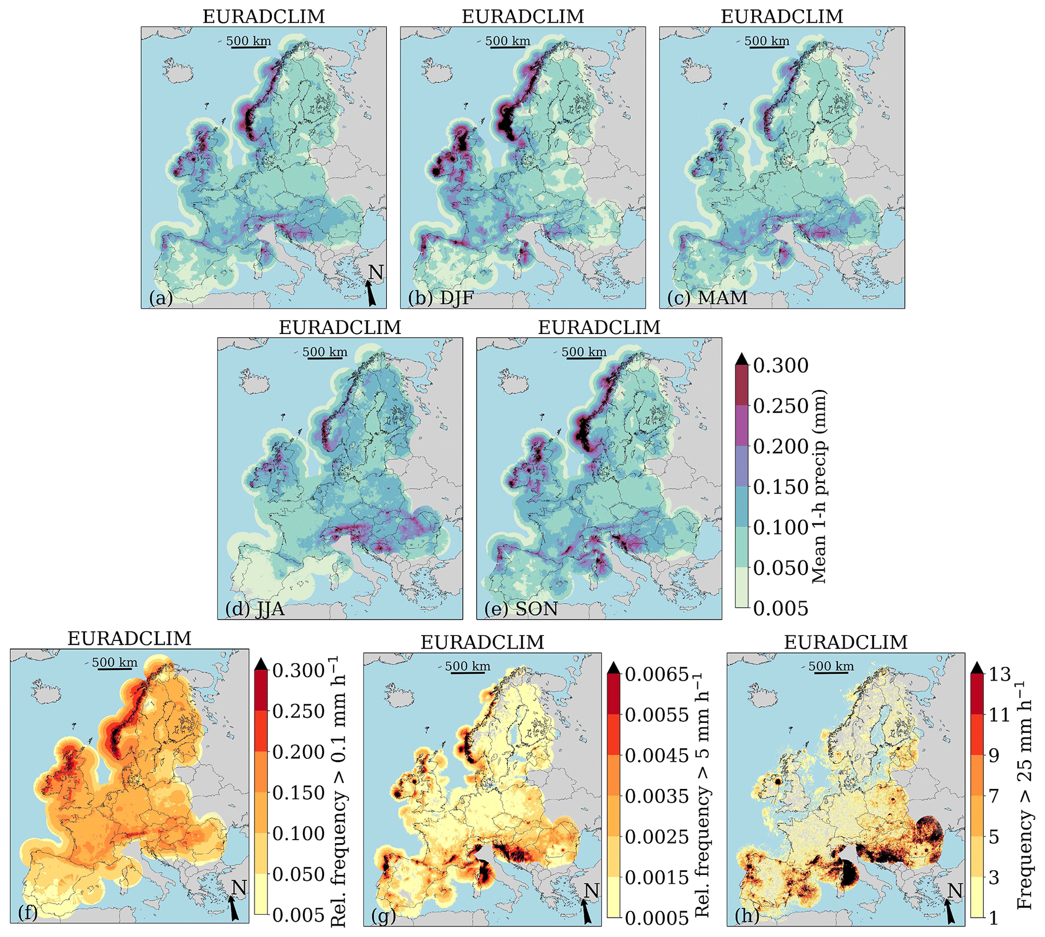
Figure 9(a)–(e) Maps of mean hourly precipitation over the entire period and per season over the period 2013–2020 (winter: December, January, February; spring: March, April, May; summer: June, July, August; fall: September, October, November). (f)–(g) Relative frequencies of exceedance of 0.1 and 5 mm, respectively, in an hour over the period 2013–2020. (h) Frequency of exceedance of 25 mm in an hour, a downpour, over the period 2013–2020. Relative frequencies of exceedance (f–g) are obtained by dividing by the number of available values for each individual radar grid cell (i.e., not equal to nodata or not missing). This implies that periods with missing radar data are not taken into account, and the number of intervals that are used will vary in space. Results are only shown for grid cells with a minimum availability of 83.3 %. Maps made with Natural Earth. Free vector and raster map data © https://naturalearthdata.com (last access: 23 March 2023).
An additional comparison is presented in Appendix B, where the eight EURADCLIM annual precipitation accumulations are compared to those from the gridded rain gauge dataset E-OBS. Generally, precipitation patterns agree, but many local differences can be found. At far range from radars and rain gauges, a decrease in annual precipitation is found (e.g., above the sea). Artifacts in radar accumulations, especially spokes caused by interference, result in overestimation in some regions. The E-OBS data are based on all days, whereas EURADCLIM has some missing data, and especially the first ∼ 3 weeks of 2013 do not have data. Note that E-OBS has a grid of 0.1∘, which is much coarser than the 2 km radar grid. More importantly, the underlying gauge network density can be sparse, whereas EURADCLIM provides full coverage. Hence, differences between EURADCLIM and E-OBS are expected, and Appendix B is meant as an illustration and sanity check for both datasets.
4.4 EURADCLIM extreme precipitation events
Figure 10 shows EURADCLIM's precipitation estimates for three extreme precipitation events meant to illustrate EURADCLIM's potential: a widespread event across Europe showing the associated precipitation pattern of an extratropical cyclone with locally more than 60 mm in 24 h (Fig. 10a), an extreme event in eastern Europe with at least 120 mm in 24 h (Fig. 10b) and a very-extreme event in southern France with at least 350 mm locally in 24 h, with at least 80 mm in the last hour (Fig. 10c–d). These events illustrate that EURADCLIM can capture extreme precipitation events across Europe, which can especially be valuable for regions where climatological radar precipitation datasets do not exist or are not open and where the affected area spans multiple countries.
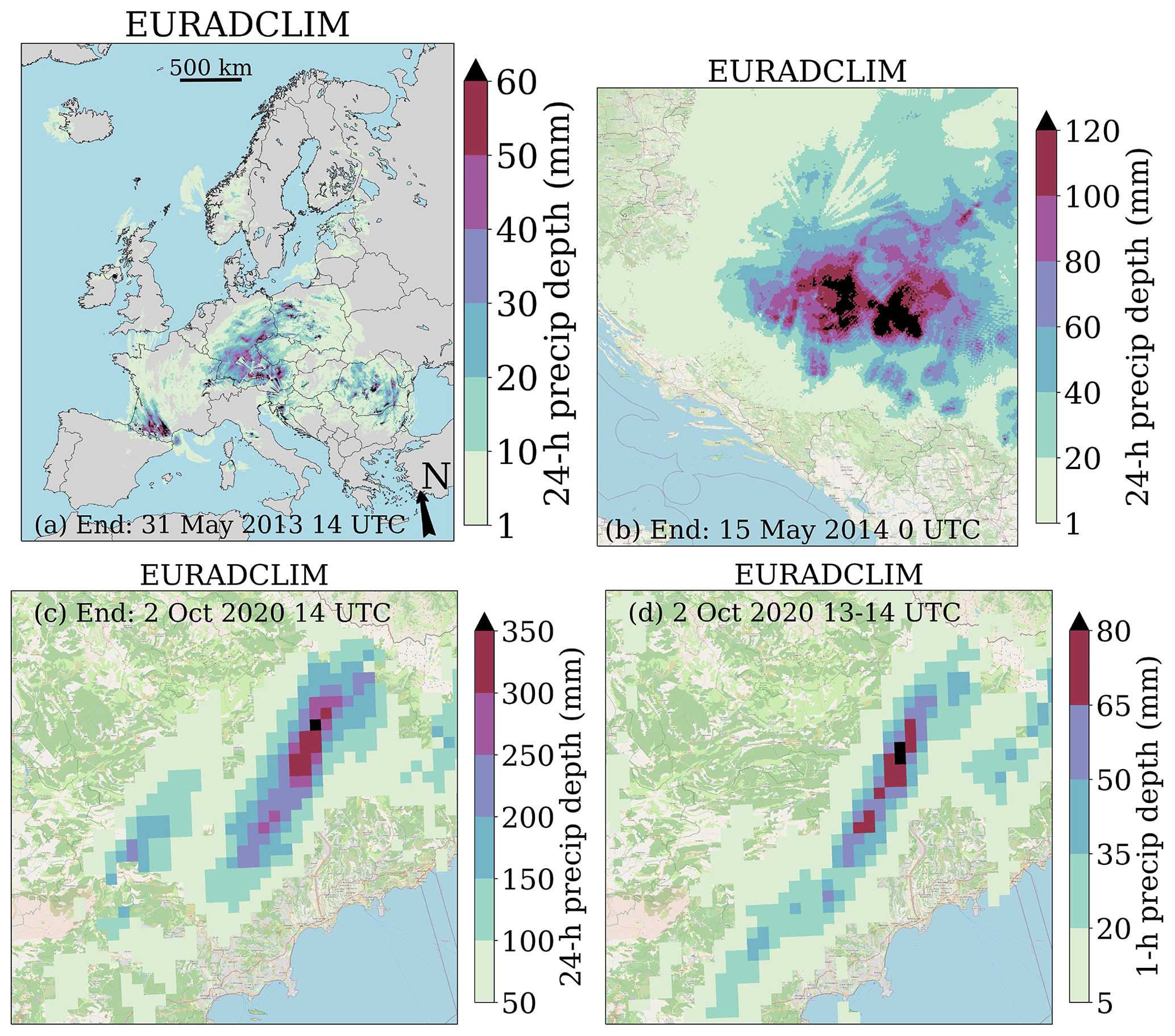
Figure 10Three precipitation events that led to flooding. (a) A widespread event over Europe from 30 May 2013 14:00 UTC to 31 May 2013 14:00 UTC (24 h precipitation accumulation), which is also presented as the Supplement (Movie S1). (b) An event in eastern Europe from 14 May 2014 00:00 UTC to 15 May 2014 00:00 UTC (24 h precipitation accumulation) and (c)–(d) a very-extreme event north of Nice, southern France, from 1 October 2020 14:00 UTC to 2 October 2020 14:00 UTC (24 h precipitation accumulation) and its last hour (1 h precipitation accumulation). (a) Map made with Natural Earth. Free vector and raster map data © https://naturalearthdata.com (last access: 23 March 2023). (b)–(d) Map data © OpenStreetMap contributors 2022. Distributed under the Open Data Commons Open Database License (ODbL) v1.0.
The EURADCLIM 1 and 24 h precipitation datasets are available from the KNMI Data Platform. The dataset of 1 h precipitation is available at https://doi.org/10.21944/7ypj-wn68 (Overeem et al., 2022a). The dataset of 24 h precipitation is available at https://doi.org/10.21944/1a54-gg96 (Overeem et al., 2022b). For each year a zip file is provided. The data are in UTC, where the time in the unzipped filenames is the end time of observation in UTC.
The following tools, written in the Python programming language (version 3), are publicly available at the GitHub repository EURADCLIM-tools (https://github.com/overeem11/EURADCLIM-tools, last access: 27 March 2023; DOI: https://doi.org/10.5281/zenodo.7473816, Overeem, 2022), to process OPERA-based radar precipitation files: a script to accumulate data, a script to perform climatological analyses (e.g., to compute the mean and the relative frequency of exceedance), two scripts to visualize precipitation and one of them with an OpenStreetMap or Google Maps as a background. This can help end-users to visualize precipitation maps and to further explore and analyze the EURADCLIM dataset.
We presented a climatological gauge-adjusted radar dataset of 1 and 24 h precipitation accumulations, EURADCLIM, covering a large part of Europe over the period 2013–2020. Clearly, EURADCLIM will not outperform national (climatological) radar precipitation datasets (e.g., Overeem et al., 2009b; Goudenhoofdt and Delobbe, 2016; Winterrath et al., 2018; Saltikoff et al., 2019a; KNMI, 2023). The spatiotemporal resolution of (the underlying) composites will often be higher, e.g., 5 min or 10 min instead of 15 min and 1 km2 instead of 4 km2. In addition, they may have undergone additional processing (e.g., based on 3D radar data) or may use more rain gauge data. These are expected to increase the accuracy of QPE with respect to EURADCLIM. However, such national datasets often do not exist or are not freely available for research or other purposes. Moreover, EURADCLIM allows users to use a common dataset for a large part of Europe instead of using different datasets from multiple countries. EURADCLIM will also benefit from possible future improvements in the OPERA surface rain rate product.
Apart from the evaluation of EURADCLIM, the performances of the OPERA precipitation product and three clutter-removal algorithms were evaluated over an 8-year period. Some of the processing steps could also be applied in (near) real time and would help to further improve the OPERA precipitation products. As is shown, the Gabella clutter filter would clearly decrease non-meteorological echoes in the OPERA product and would be directly applicable. OPERA already uses a satellite cloud mask. The static clutter mask could be applied if the annual precipitation accumulations from the previous year were used. When subdaily near-real-time gauge accumulations become available, this would pave the way for merging with OPERA radar accumulations in near real time, e.g., by merging data from the last clock hour. We think this would be a useful improvement to the product developed by Park et al. (2019). The correction for the motion of the precipitation field from Park et al. (2019) could be a valuable addition to EURADCLIM. Moreover, in line with Park et al. (2019), the temporal resolution of EURADCLIM could be increased to 15 min. Finally, the period of evaluation by Park et al. (2019) of the OPERA-based QPE as a function of time could be extended, and this daily monitoring could also be applied to EURADCLIM.
This first version of EURADCLIM should be seen as a starting point. Despite the different algorithms to remove non-meteorological echoes applied by NMHSs, OPERA and EURADCLIM, these echoes do still pose a problem. We claim that precipitation climatologies derived from EURADCLIM have a reasonable accuracy and that extreme events can be captured at a much higher spatiotemporal resolution but that EURADCLIM is not directly suited yet for extreme-value modeling at the grid cell scale, which requires records of the most extreme events, such as annual maxima. EURADCLIM may already be suitable for extreme-value modeling in the case of longer durations or larger-area sizes than the grid cell scale, such as larger hydrological catchments. Then non-meteorological echoes may average out. We also recommend comparing the EURADCLIM precipitation accumulations to those from national radar datasets, specifically to assess the performance of EURADCLIM in capturing extreme precipitation.
Outliers, such as presented in Fig. 8 and visible in the frequency of downpours (Fig. 9h), limit the applicability of EURADCLIM at the grid cell scale, especially for use in extreme value modeling (e.g., Frederick et al., 1977; Durrans et al., 2002; Allen and DeGaetano, 2005; Overeem et al., 2009a, 2010; Marra and Morin, 2015; McGraw et al., 2019). Here, we provide some recommendations to end-users for dealing with these outliers.
-
One way of dealing with this is to apply an algorithm that does not take into account entire composites that have severe artifacts over larger areas. These could be automatically identified by radar–gauge comparison, possibly followed by a visual inspection and selection. For instance, the number of grid cells with a large ratio between gauge and radar accumulations could be counted. If the total count exceeds a threshold, the interval can be labeled as suspicious.
-
Another approach would be to set grid cells above a certain threshold to a lower (e.g., interpolated) value or always discard such a grid cell if it experienced such a high value at least once during the period 2013–2020. A drawback of this approach is that such a threshold is a bit arbitrary and that it influences the statistics of extreme precipitation. For example, grid cells with annual precipitation clearly above that of local climatological gauge records could be discarded as well as grid cells with unlikely high values for 24 h precipitation.
QPE could be further improved, especially in areas with sparse rain gauge network density or far away from weather radars. Some regions are far away from rain gauges, making the merging algorithm less effective. In some cases no merging is even carried out because of the long distance to the nearest rain gauge (e.g., Iceland, Malta). To improve the quality of EURADCLIM but also the OPERA near-real-time precipitation products, we provide the following main recommendations for NMHSs, the OPERA program and EURADCLIM.
-
Start with the volumetric radar data, and apply algorithms (Goudenhoofdt and Delobbe, 2016) such as fuzzy-logic clutter removal (Berenguer et al., 2006; Gourley et al., 2007; Crisologo et al., 2014; Krause, 2016; Overeem et al., 2020), attenuation correction (Carey et al., 2000; Testud et al., 2000; Vulpiani et al., 2012; Al-Sakka et al., 2013; Jacobi and Heistermann, 2016; Overeem et al., 2021) and the vertical profile of reflectivity correction (Hazenberg et al., 2013). The use of polarimetric variables would especially add value, also in the conversion to rain rates. Moreover, differences between weather radars, e.g., polarimetric or not, and climate would require careful local analyses and optimization of parameters (e.g., fuzzy-logic settings, precipitation retrieval relations for rain/snow).
-
Obtain gauge data from more locations and update the rain gauge records that overlap with the (extended) EURADCLIM time span. Additional high-quality data might come from, e.g., NMHSs, water and river authorities and other data-holding institutes. Instead of using only daily data, ideally clock-hourly data would also become available, which would avoid possible errors introduced by disaggregating daily precipitation. These are desirable given the often large spatial and temporal variability in precipitation and in sources of error in radar QPE.
-
Specifically, third-party data could be employed after appropriate quality-control (and retrieval) algorithms have been applied. This also requires efforts from NMHSs to bring these from research to operations (Garcia-Marti et al., 2023). Examples of such third-party data sources are rain gauge data from personal weather stations (PWSs) connected to the Internet (De Vos et al., 2019; Graf et al., 2021) and commercial microwave link (CML) data (Messer et al., 2006; Leijnse et al., 2007; Overeem et al., 2016; Graf et al., 2020, 2021). The merging of these kinds of datasets with radar data is studied in the COST Action OpenSense (https://opensenseaction.eu/, last access: 23 March 2023). These data sources could potentially be available in (near) real time and would give a vast increase in the density of surface precipitation estimates. However, the increase over time in the number of available third-party data challenges the aim of EURADCLIM to provide a climatic perspective of hourly rainfall.
-
Develop a radar–gauge merging algorithm that takes into account the local rain gauge network density. For the current method, the local mean-field bias adjustment followed by a spatial adjustment could then be replaced by a spatial adjustment where the value of the short-range parameter rs varies seamlessly in space as a function of network density. In addition, the value of the short-range parameter should be based on the local precipitation climatology instead of on the precipitation climatology from the Netherlands. Also, other adjustment methods could be evaluated (Goudenhoofdt and Delobbe, 2009).
-
Add uncertainty information to radar and gauge data, and use this in the radar–gauge merging, for instance, by using the OPERA quality index and additional information on the radar quality and the rain gauge network density. Alternatively, it could be studied whether a meaningful relationship can be established between the quality of EURADCLIM and the distance to the nearest gauge or radar. Then maps with the distance to the nearest gauge or radar (Fig. 2c–d) could guide the user in judging the suitability of using a certain grid cell or region of EURADCLIM for a given application. Ideally, such quality maps would be computed for each 1 h interval, taking into account the gauges actually used in the merging and the radar coverage and quality for that time interval. To facilitate this, we recommend adding the actual radar coordinates for each individual time interval to the OPERA products.
-
A more sophisticated approach would be to remove more non-meteorological echoes by applying a satellite cloud mask that employs cloud optical thickness, i.e., also in the case of thicker non-precipitating clouds.
-
Finally, in the future, MSG will be replaced by the Meteosat Third Generation that allows for a more local correction due to higher spatial and temporal resolution, provided parallax effects are accounted for.
EURADCLIM's strategic value encompasses the following.
-
There is a much better reference for validation of weather prediction model output (e.g., HARMONIE/ECMWF) (Van der Plas et al., 2017), regional climate model simulations (Berg et al., 2019), satellite precipitation products (Skofronick‐Jackson et al., 2018; Sun et al., 2018) and opportunistic sensing data (e.g., CMLs and PWSs), which allows for improvement of their quality control or retrieval algorithms.
-
It allows for better monitoring of (trends in) precipitation extremes and their spatial extent, except for the most extreme events at the grid cell scale, such as annual maxima, due to the remaining non-meteorological echoes. This facilitates better understanding of the drivers behind such events (e.g., the relation to dew point temperature, atmospheric circulation, diurnal cycle and clustering of showers) and climate attribution (Lochbihler et al., 2017; Lengfeld et al., 2019). Deriving a catalog of extreme precipitation events becomes possible, as is done for Germany by Lengfeld et al. (2021). This is all highly relevant for anticipating future extremes in a changing climate.
-
It allows for better evaluation of extreme precipitation events and their impact (e.g., landslides, flooding), specifically, use as input for hydrological models in order to improve these models, especially for flash flood forecasting.
We expect to rerun EURADCLIM once a year over the entire period, using all available ECA&D rain gauge data, and extend it with 1 year of data. This will result in a new version of this dataset. Hence, we invite NMHSs or other institutes to make all their rain gauge data available to ECA&D. We encourage one to start using EURADCLIM and discover its value and shortcomings for a variety of applications, and we appreciate any feedback on this. It is expected that EURADCLIM will be of use to various (scientific) domains and applications and that future collaborations and funding will lead to improved next versions of EURADCLIM.
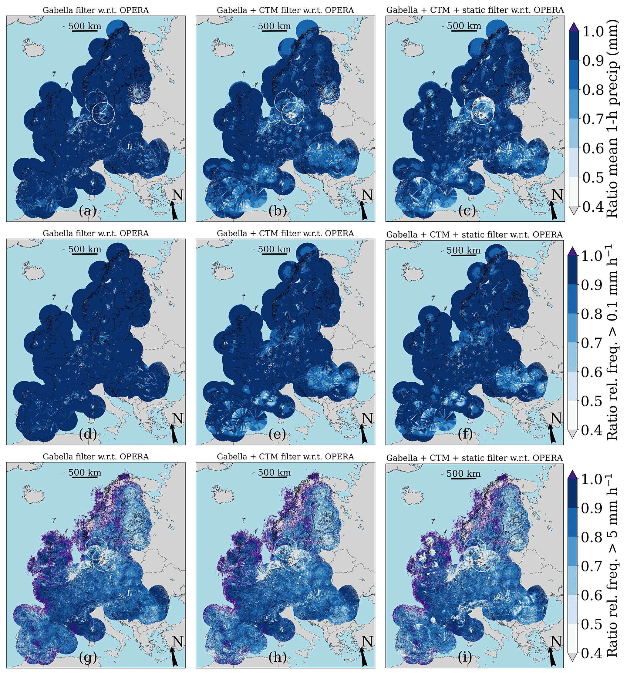
Figure A1Comparison between 1 h precipitation accumulations from three datasets to study the effect of non-meteorological echo removal algorithms over the period 2013–2020. (a)–(c) Maps of the ratio of mean hourly precipitation with respect to the OPERA dataset and (d)–(i) maps of the ratio of the relative frequency of exceedance of 0.1 and 5 mm in an hour with respect to the OPERA dataset. The purple areas imply that the ratio is 1. The uncolored areas do not have data or have a relative frequency of 0 for one or both datasets. Map made with Natural Earth. Free vector and raster map data © https://naturalearthdata.com (last access: 23 March 2023).
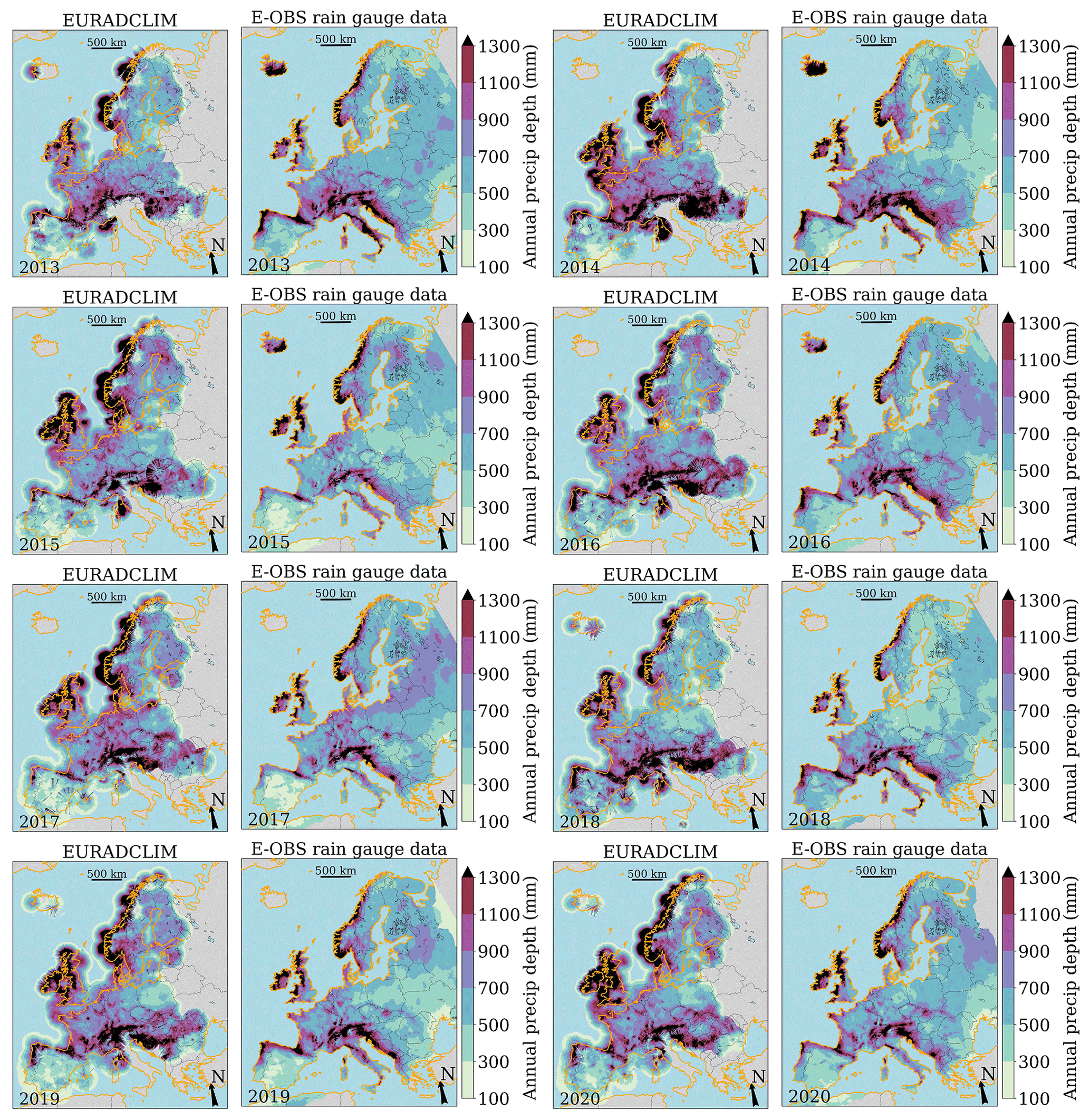
Figure B1Annual precipitation accumulations over the period 2013–2020 for EURADCLIM (4 km2) and interpolated rain gauge observations (E-OBS version 25.0e; release April 2022; , which is ∼11 km in latitude and ∼4–9 km in longitude, depending on the latitude). Coastlines are plotted in orange to ease the comparison between EURADCLIM and E-OBS, due to the coverage above open water by radars for which E-OBS does not provide precipitation estimates. Map made with Natural Earth. Free vector and raster map data © https://naturalearthdata.com (last access: 23 March 2023).
The supplemental video (Movie S1) visualizes a widespread precipitation event on 30 and 31 May 2013 over Europe that led to flooding. The supplement related to this article is available online at: https://doi.org/10.5194/essd-15-1441-2023-supplement.
Author contributions are captured following the CRediT system. Conceptualization: AO, GvdS and HL. Data curation: AO, EvdB, GvdS and JFM. Formal analysis: AO. Funding acquisition: AO, EvdP, GvdS, HL and JFM. Investigation: AO, EvdB and GvdS. Methodology: AO, GvdS, HL and JFM. Project administration: AO. Software: AO, HL and JFM. Supervision: AO and HL. Validation by AO and EvdP. Visualization: AO. Writing – original draft preparation: AO and HL. Writing – review and editing: AO, EvdB, EvdP, GvdS, JFM and HL.
The contact author has declared that none of the authors has any competing interests.
Publisher’s note: Copernicus Publications remains neutral with regard to jurisdictional claims in published maps and institutional affiliations.
We thank Martin Stengel (Deutscher Wetterdienst) for providing the CLAAS-2 satellite product and thank EUMETSAT. We are grateful for the E-OBS dataset (Cornes et al., 2018) from the EU-FP6 project Uncertainties in Ensembles of Regional ReAnalyses (https://www.uerra.eu, last access: 23 March 2023), the Copernicus Climate Change Service, the data providers in the ECA&D project (https://www.ecad.eu, last access: 23 March 2023) and the NMHSs, who provided radar data to OPERA. We are grateful to Annakaisa von Lerber (Finnish Meteorological Institute, the OPERA program manager), Willie McCairns MBA FRMetS (ECOMET, an economic interest grouping of the National Meteorological Services of the European Economic Area, Chief Executive) and Annelies Demolder (ECOMET) for their efforts in making the EURADCLIM dataset public. We thank two anonymous reviewers for their constructive comments. The website of the project can be found at https://www.knmi.nl/research/observations-data-technology/projects/euradclim-the-european-climatological-high-resolution-gauge-adjusted-radar-rainfall-dataset (last access: 23 March 2023). All figures containing maps were made with the Python package Cartopy (Met Office, 2022).
This research has been supported by the Royal Netherlands Meteorological Institute's multi-annual strategic research program (project no. 2017.02).
This paper was edited by Alexander Gruber and reviewed by two anonymous referees.
Al-Sakka, H., Boumahmoud, A.-A., Fradon, B., Frasier, S. J., and Tabary, P.: A new fuzzy logic hydrometeor classification scheme applied to the French X-, C-, and S-band polarimetric radars, J. Appl. Meteorol. Clim., 52, 2328–2344, https://doi.org/10.1175/JAMC-D-12-0236.1, 2013. a
Allen, R. J. and DeGaetano, A. T.: Considerations for the use of radar-derived precipitation estimates in determining return intervals for extreme areal precipitation amounts, J. Hydrol., 315, 203–219, https://doi.org/10.1016/j.jhydrol.2005.03.028, 2005. a
Barnes, S. L.: A technique for maximizing details in numerical weather map analysis, J. Appl. Meteorol., 3, 396–409, 1964. a
Barton, Y., Sideris, I., Raupach, T., Gabella, M., Germann, U., and Martius, O.: A multi-year assessment of sub-hourly gridded precipitation for Switzerland based on a blended radar–Rain-gauge dataset, Int. J. Climatol., 40, 5208–5222, https://doi.org/10.1002/joc.6514, 2020. a
Benas, N., Finkensieper, S., Stengel, M., van Zadelhoff, G.-J., Hanschmann, T., Hollmann, R., and Meirink, J. F.: The MSG-SEVIRI-based cloud property data record CLAAS-2, Earth Syst. Sci. Data, 9, 415–-434, https://doi.org/10.5194/essd-9-415-2017, 2017. a
Berenguer, M., Sempere-Torres, D., Corral, C., and Sánchez-Diezma, R.: A fuzzy logic technique for identifying nonprecipitating echoes in radar scans, J. Atmos. Ocean. Tech., 23, 1157–1180, https://doi.org/10.1175/JTECH1914.1, 2006. a
Berg, P., Christensen, O. B., Klehmet, K., Lenderink, G., Olsson, J., Teichmann, C., and Yang, W.: Summertime precipitation extremes in a EURO-CORDEX 0.11∘ ensemble at an hourly resolution, Nat. Hazards Earth Syst. Sci., 19, 957–971, https://doi.org/10.5194/nhess-19-957-2019, 2019. a
Bližňák, V., Kašpar, M., and Müller, M.: Radar-based summer precipitation climatology of the Czech Republic, Int. J. Climatol., 38, 677–691, https://doi.org/10.1002/joc.5202, 2018. a
Carey, L. D., Rutledge, S. A., Ahijevych, D. A., and Keenan, T. D.: Correcting propagation effects in C-band polarimetric radar observations of tropical convection using differential propagation phase, J. Appl. Meteorol., 39, 1405–1433, https://doi.org/10.1175/1520-0450(2000)039<1405:CPEICB>2.0.CO;2, 2000. a
Cornes, R. C., Van der Schrier, G., Van den Besselaar, E. J. M., and Jones, P. D.: An ensemble version of the E-OBS temperature and precipitation data sets, J. Geophys. Res.-Atmos., 123, 9391–9409, https://doi.org/10.1029/2017JD028200, 2018. a, b, c
Crisologo, I., Vulpiani, G., Abon, C. C., David, C. P. C., Bronstert, A., and Heistermann, M.: Polarimetric rainfall retrieval from a C-band weather radar in a tropical environment (the Philippines), Asia-Pac. J. Atmos. Sci., 50, 43–55, https://doi.org/10.1007/s13143-014-0049-y, 2014. a
De Vos, L. W., Leijnse, H., Overeem, A., and Uijlenhoet, R.: Quality control for crowdsourced personal weather stations to enable operational rainfall monitoring, Geophys. Res. Lett., 46, 8820–8829, https://doi.org/10.1029/2019GL083731, 2019. a
Derrien, M. and Le Gléau, H.: MSG/SEVIRI cloud mask and type from SAFNWC, Int. J. Remote Sens., 26, 4707–4732, 2005. a
Doviak, R. J. and Zrnić, D. S.: Doppler Radar and Weather Observations, second edn., Dover Publications, Inc., Mineola, New York, ISBN 0-486-45060-0, 1993. a
Durrans, S. R., Julian, L. T., and Yekta, M.: Estimation of depth-area relationships using radar-rainfall data, J. Hydrol. Eng., 7, 356–367, https://doi.org/10.1061/(ASCE)1084-0699(2002)7:5(356), 2002. a
Fabry, F.: Radar Meteorology: Principles and Practice, Cambridge University Press, Cambridge, U.K., https://doi.org/10.1017/CBO9781107707405, 2015. a, b
Fabry, F., Meunier, V., Treserras, B. P., Cournoyer, A., and Nelson, B.: On the climatological use of radar data mosaics: possibilities and challenges, B. Am. Meteorol. Soc., 98, 2135–2148, https://doi.org/10.1175/BAMS-D-15-00256.1, 2017. a, b
Finkensieper, S., Meirink, J.-F., van Zadelhoff, G.-J., Hanschmann, T., Benas, N., Stengel, M., Fuchs, P., Hollmann, R., and Werscheck, M.: CLAAS-2: CM SAF CLoud property dAtAset using SEVIRI – Edition 2, Satellite Application Facility on Climate Monitoring, https://doi.org/10.5676/EUM_SAF_CM/CLAAS/V002, 2016. a
Frech, M., Hagen, M., and Mammen, T.: Monitoring the absolute calibration of a polarimetric weather radar, J. Atmos. Ocean. Tech., 34, 599–615, https://doi.org/10.1175/JTECH-D-16-0076.1, 2017. a
Frederick, R. H., Myers, V. A., and Auciello, E. P.: Storm depth-area relations from digitized radar returns, Water Resour. Res., 13, 675–679, 1977. a
Gabella, M. and Notarpietro, R.: Ground clutter characterization and elimination in mountainous terrain, in: Proceedings of the 2nd European conference on radar meteorology ERAD and the COST 717 mid-term seminar, https://www.copernicus.org/erad/online/erad-305.pdf (last access: 23 March 2023), 2002. a, b
Garcia-Marti, I., Overeem, A., Noteboom, J. W., de Vos, L., de Haij, M., and Whan, K.: From proof-of-concept to proof-of-value: approaching third-party data to operational workflows of national meteorological services, Int. J. Climatol., 43, 275–292, https://doi.org/10.1002/joc.7757, 2023. a
Goudenhoofdt, E. and Delobbe, L.: Evaluation of radar-gauge merging methods for quantitative precipitation estimates, Hydrol. Earth Syst. Sci., 13, 195–203, https://doi.org/10.5194/hess-13-195-2009, 2009. a
Goudenhoofdt, E. and Delobbe, L.: Generation and verification of rainfall estimates from 10-yr volumetric weather radar measurements, J. Hydrometeorol., 17, 1223–1242, https://doi.org/10.1175/JHM-D-15-0166.1, 2016. a, b, c
Gourley, J. J., Tabary, P., and Parent du Chatelet, J.: A fuzzy logic algorithm for the separation of precipitating from nonprecipitating echoes using polarimetric radar observations, J. Atmos. Ocean. Tech., 24, 1439–1451, https://doi.org/10.1175/JTECH2035.1, 2007. a, b
Graf, M., Chwala, C., Polz, J., and Kunstmann, H.: Rainfall estimation from a German-wide commercial microwave link network: optimized processing and validation for 1 year of data, Hydrol. Earth Syst. Sci., 24, 2931–2950, https://doi.org/10.5194/hess-24-2931-2020, 2020. a
Graf, M., El Hachem, A., Eisele, M., Seidel, J., Chwala, C., Kunstmann, H., and Bárdossy, A.: Rainfall estimates from opportunistic sensors in Germany across spatio-temporal scales, J. Hydrol.: Regional Studies, 37, 1448–1463, https://doi.org/10.1016/j.ejrh.2021.100883, 2021. a, b
Hazenberg, P., Torfs, P. J. J. F., Leijnse, H., Delrieu, G., and Uijlenhoet, R.: Identification and uncertainty estimation of vertical reflectivity profiles using a Lagrangian approach to support quantitative precipitation measurements by weather radar, J. Geophys. Res.-Atmospheres, 118, 10243–10261, https://doi.org/10.1002/jgrd.50726, 2013. a, b
Heistermann, M., Jacobi, S., and Pfaff, T.: Technical Note: An open source library for processing weather radar data (wradlib), Hydrol. Earth Syst. Sci., 17, 863–871, https://doi.org/10.5194/hess-17-863-2013, 2013. a, b
Hitschfeld, W. and Bordan, J.: Errors inherent in the radar measurement of rainfall at attenuating wavelengths, J. Meteorol., 11, 58–67, https://doi.org/10.1175/1520-0469(1954)011<0058:EIITRM>2.0.CO;2, 1954. a
Holleman, I.: Bias adjustment and long-term verification of radar-based precipitation estimates, Meteor. Appl., 14, 195–203, https://doi.org/10.1002/met.22, 2007. a
Huuskonen, A., Saltikoff, E., and Holleman, I.: The operational weather radar network in Europe, B. Am. Meteorol. Soc., 95, 897–907, https://doi.org/10.1175/BAMS-D-12-00216.1, 2014. a
Jacobi, S. and Heistermann, M.: Benchmarking attenuation correction procedures for six years of single-polarized C-band weather radar observations in South-West Germany, Geomat. Nat. Haz. Risk, 7, 1785–1799, https://doi.org/10.1080/19475705.2016.1155080, 2016. a, b
Kitchen, M. and Blackall, R. M.: Representativeness errors in comparisons between radar and gauge measurements of rainfall, J. Hydrol., 134, 13–33, 1992. a
Klein Tank, A. M. G., Wijngaard, J. B., Können, G. P., et al.: Daily dataset of 20th-century surface air temperature and precipitation series for the European Climate Assessment, Int. J. Climatol., 22, 1441–1453, https://doi.org/10.1002/joc.773, 2002. a
Klok, E. J. and Klein Tank, A. M. G.: Updated and extended European dataset of daily climate observation, Int. J. Climatol., 29, 1182–1191, https://doi.org/10.1002/joc.1779, 2008. a
KNMI: Precipitation – 5 minute precipitation accumulations from climatological gauge-adjusted radar dataset for The Netherlands (1 km, extended mask) in KNMI HDF5 format, KNMI Data Platform [data set], https://dataplatform.knmi.nl/dataset/rad-nl25-rac-mfbs-em-5min-2-0, last access: 27 March 2023. a
Krause, J. M.: A simple algorithm to discriminate between meteorological and nonmeteorological radar echoes, J. Atmos. Ocean. Tech., 33, 1875–1885, https://doi.org/10.1175/JTECH-D-15-0239.1, 2016. a
Leijnse, H., Uijlenhoet, R., and Stricker, J. N. M.: Rainfall measurement using radio links from cellular communication networks, Water Resour. Res., 43, W03201, https://doi.org/10.1029/2006WR005631, 2007. a
Lengfeld, K., Winterrath, T., Junghänel, T., Hafer, M., and Becker, A.: Characteristic spatial extent of hourly and daily precipitation events in Germany derived from 16 years of radar data, Meteorol. Z., 28, 363–378, https://doi.org/10.1127/metz/2019/0964, 2019. a
Lengfeld, K., Walawender, E., Winterrath, T., and Becker, A.: CatRaRE: A Catalogue of radar-based heavy rainfall events in Germany derived from 20 years of data, Meteorol. Z., 30, 469–487, https://doi.org/10.1127/metz/2021/1088, 2021. a
Lochbihler, K., Lenderink, G., and Siebesma, A. P.: The spatial extent of rainfall events and its relation to precipitation scaling, Geophys. Res. Lett., 44, 8629–8636, https://doi.org/10.1002/2017GL074857, 2017. a
Marra, F. and Morin, E.: Use of radar QPE for the derivation of Intensity–Duration–Frequency curves in a range of climatic regimes, J. Hydrol., 531, 427–440, https://doi.org/10.1016/j.jhydrol.2015.08.064, 2015. a
McGraw, D., Nikolopoulos, E. I., Marra, F., and Anagnostou, E. N.: Precipitation frequency analyses based on radar estimates: An evaluation over the contiguous United States, J. Hydrol., 573, 299–310, https://doi.org/10.1016/j.jhydrol.2019.03.032, 2019. a
Messer, H. A., Zinevich, A., and Alpert, P.: Environmental monitoring by wireless communication networks, Science, 312, 713, https://doi.org/10.1126/science.1120034, 2006. a
Met Office: Cartopy: a cartographic python library with a Matplotlib interface, https://scitools.org.uk/cartopy (last access: 23 March 2023), 2022. a
Michelson, D. B., Lewandowski, R., Szewczykowski, M., Beekhuis, H., Haase, G., Mammen, T., Faure, D., Simpson, M., Leijnse, H., and Johnson, D.: EUMETNET OPERA weather radar information model for implementation with the HDF5 file format Version 2.3, EUMETNET OPERA, https://www.eumetnet.eu/wp-content/uploads/2019/01/ODIM_H5_v23.pdf (last access: 23 March 2023), 2019. a, b, c
Mühlbauer, K., Heistermann, M., and Goudenhoofdt, E.: wradlib/wradlib: wradlib release v1.9.0 (1.9.0), Zenodo [code], https://doi.org/10.5281/zenodo.4290240, 2020. a, b
Nelson, B. R., Prat, O. P., Seo, D.-J., and Habib, E.: Assessment and implications of NCEP Stage IV quantitative precipitation estimates for product intercomparisons, Weather Forecast., 31, 371–394, https://doi.org/10.1175/WAF-D-14-00112.1, 2016. a
NWC SAF: Algorithm Theoretical Basis Document for ”Cloud Products” (CMa-PGE01 v3.2, CT-PGE02 v2.2 & CTTH-PGE03 v2.2), Tech. Rep. SAF/NWC/CDOP2/MFL/SCI/ATBD/01, Issue 3, Rev. 2.1, EUMETSAT Satellite Application Facility on Nowcasting and Short range Forecasting, https://www.nwcsaf.org/AemetWebContents/ScientificDocumentation/Documentation/MSG/SAF-NWC-CDOP2-MFL-SCI-ATBD-01_v3.2.1.pdf (last access: 27 March 2023), 2013. a
OPERA: OPERA – Eumetnet, https://www.eumetnet.eu/activities/observations-programme/current-activities/opera/ (last access: 23 March 2023), 2022. a
Overeem, A.: EURADCLIM-tools (v.1.0), Zenodo [code], https://doi.org/10.5281/zenodo.7473816, 2022. a
Overeem, A., Buishand, T. A., and Holleman, I.: Extreme rainfall analysis and estimation of depth-duration-frequency curves using weather radar, Water Resour. Res., 45, W10424, https://doi.org/10.1029/2009WR007869, 2009a. a
Overeem, A., Holleman, I., and Buishand, A.: Derivation of a 10-year radar-based climatology of rainfall, J. Appl. Meteorol. Clim., 48, 1448–1463, https://doi.org/10.1175/2009JAMC1954.1, 2009b. a, b
Overeem, A., Buishand, T. A., Holleman, I., and Uijlenhoet, R.: Extreme value modeling of areal rainfall from weather radar, Water Resour. Res., 46, W09514, https://doi.org/10.1029/2009WR008517, 2010. a
Overeem, A., Leijnse, H., and Uijlenhoet, R.: Two and a half years of country‐wide rainfall maps using radio links from commercial cellular telecommunication networks, Water Resour. Res., 52, 8039–8065, https://doi.org/10.1002/2016WR019412, 2016. a
Overeem, A., Uijlenhoet, R., and Leijnse, H.: Full-year evaluation of non-meteorological echo removal with dual-polarization fuzzy logic for two C-band radars in a temperate climate, J. Atmos. Ocean. Tech., 37, 1643–1660, https://doi.org/10.1175/JTECH-D-19-0149.1, 2020. a, b
Overeem, A., de Vries, H., Al Sakka, H., Uijlenhoet, R., and Leijnse, H.: Rainfall-induced attenuation correction for two operational dual-polarization C-band radars in the Netherlands, J. Atmos. Ocean. Tech., 38, 1125–1142, https://doi.org/10.1175/JTECH-D-20-0113.1, 2021. a, b
Overeem, A., van den Besselaar, E., van der Schrier, G., Meirink, J., van der Plas, E., and Leijnse, H.: EURADCLIM: The European climatological gauge-adjusted radar precipitation dataset (1-h accumulations), KNMI Data Platform [data set], https://doi.org/10.21944/7ypj-wn68, 2022a. a, b
Overeem, A., van den Besselaar, E., van der Schrier, G., Meirink, J., van der Plas, E., and Leijnse, H.: EURADCLIM: The European climatological gauge-adjusted radar precipitation dataset (24-h accumulations), KNMI Data Platform [data set], https://doi.org/10.21944/1a54-gg96, 2022b. a, b
Park, S., Berenguer, M., and Sempere-Torres, D.: Long-term analysis of gauge-adjusted radar rainfall accumulations at European scale, J. Hydrol., 573, 768–777, https://doi.org/10.1016/j.jhydrol.2019.03.093, 2019. a, b, c, d, e, f, g, h
Project team ECA&D and Royal Netherlands Meteorological Institute KNMI: European Climate Assessment & Dataset (ECA&D), Algorithm Theoretical Basis Document (ATBD), Version 11, https://knmi-ecad-assets-prd.s3.amazonaws.com/documents/atbd.pdf (last access: 23 March 2023), 2021. a
Rauber, R. M. and Nesbitt, S. L.: Radar Meteorology: A First Course, John Wiley & Sons, Hoboken, NJ, USA, https://doi.org/10.1002/9781118432662, 2018. a
Ryzhkov, A. V. and Zrnic, D. S.: Radar Polarimetry for Weather Observations, Springer Nature Switzerland AG, Cham, Switzerland, https://doi.org/10.1007/978-3-030-05093-1, 2019. a
Saltikoff, E., Cho, J. Y. N., Tristant, P., Huuskonen, A., Allmon, L., Cook, R., Becker, E., and Joe, P.: The threat to weather radars by wireless technology, B. Am. Meteorol. Soc., 97, 1159–1167, https://doi.org/10.1175/BAMS-D-15-00048.1, 2016. a
Saltikoff, E., Friedrich, K., Soderholm, J., Lengfeld, K., Nelson, B., Becker, A., Hollmann, R., Urban, B., Heistermann, M., and Tassone, C.: An overview of using weather radar for climatological studies: successes, challenges, and potential, B. Am. Meteorol. Soc., 100, 1739–1752, https://doi.org/10.1175/BAMS-D-18-0166.1, 2019a. a
Saltikoff, E., Haase, G., Delobbe, L., Gaussiat, N., Martet, M., Idziorek, D., Leijnse, H., Novák, P., Lukach, M., and Stephan, K.: OPERA the radar project, Atmosphere, 10, 320, https://doi.org/10.3390/atmos10060320, 2019b. a, b
Skofronick‐Jackson, G., Kirschbaum, D., Petersen, W., Huffman, G., Kidd, C., Stocker, E., and Kakar, R.: The Global Precipitation Measurement (GPM) mission's scientific achievements and societal contributions: reviewing four years of advanced rain and snow observations, Q. J. Roy. Meteorol. Soc., 144, 27–48, https://doi.org/10.1002/qj.3313, 2018. a
Sun, Q., Miao, C., Duan, Q., Ashouri, H., Sorooshian, S., and Hsu, K.-L.: A review of global precipitation data sets: data sources, estimation, and intercomparisons, Rev. Geophys., 56, 79–107, https://doi.org/10.1002/2017RG000574, 2018. a
Tabary, P., Vulpiani, G., Gourley, J. J., Illingworth, A. J., Thompson, R. J., and Bousquet, O.: Unusually high differential attenuation at C Band: results from a two-year analysis of the French Trappes polarimetric radar data, J. Appl. Meteorol. Clim., 48, 2037–2053, https://doi.org/10.1175/2009JAMC2039.1, 2009. a
Testud, J., Le Bouar, E., Obligis, E., and Ali-Mehenni, M.: The rain profiling algorithm applied to polarimetric weather radar, J. Atmos. Oceanic Technol., 17, 332–356, https://doi.org/10.1175/1520-0426(2000)017<0332:TRPAAT>2.0.CO;2, 2000. a
Van de Beek, C. Z., Leijnse, H., Torfs, P. J. J. F., and Uijlenhoet, R.: Seasonal semi-variance of Dutch rainfall at hourly to daily scales, Adv. Water Resour., 45, 76–85, https://doi.org/10.1016/j.advwatres.2012.03.023, 2012. a, b
Van der Plas, E., Schmeits, M., Hooijman, N., and Kok, K.: A comparative verification of high-resolution precipitation forecasts using model output statistics, Mon. Weather Rev., 145, 4037–4054, https://doi.org/10.1175/MWR-D-16-0256.1, 2017. a
Vulpiani, G., Montopoli, M., Passeri, L. D., Gioia, A. G., Giordano, P., and Marzano, F. S.: On the use of dual-polarized C-band radar for operational rainfall retrieval in mountainous areas, J. Appl. Meteorol. Clim., 51, 405–425, https://doi.org/10.1175/JAMC-D-10-05024.1, 2012. a
Winterrath, T., Brendel, C., Hafer, M., Junghänel, T., Klameth, A., Lengfeld, K., Walawender, E., Weigl, E., and Becker, A.: RADKLIM Version 2017.002: Reprocessed gauge-adjusted radar data, one-hour precipitation sums (RW), DWD [data set], https://doi.org/10.5676/DWD/RADKLIM_RW_V2017.002, 2018. a, b
Wradlib: wradlib.clutter.filter_gabella, wradlib, https://docs.wradlib.org/en/stable/generated/wradlib.clutter.filter_gabella.html?highlight=gabella (last access: 23 March 2023), 2021. a, b
Wradlib: wradlib.clutter.histo_cut, wradlib, https://docs.wradlib.org/en/stable/generated/wradlib.clutter.histo_cut.html (last access: 23 March 2023), 2022. a
- Abstract
- Introduction
- Data
- Methodology
- Results
- Data availability
- Code availability
- Conclusions
- Appendix A: Effect of additional clutter-removal algorithms on 1 h precipitation
- Appendix B: Annual precipitation: EURADCLIM versus E-OBS
- Author contributions
- Competing interests
- Disclaimer
- Acknowledgements
- Financial support
- Review statement
- References
- Supplement