Estimating local agricultural gross domestic product (AgGDP) across the world

Economic statistics are frequently produced at an administrative level such as the subnational division. However, these measures may lack sufficient local variation for effective analysis of local economic development patterns and exposure to natural hazards. Agricultural gross domestic product (GDP) is a critical indicator for measurement of the primary sector, on which more than 2.5 billion people depend for their livelihoods, and it provides a key source of income for the entire household (FAO, 2021). Through a data-fusion method based on cross-entropy optimization, this paper disaggregates national and subnational administrative statistics of agricultural GDP into a global gridded dataset at approximately 10×10 km for the year 2010 using satellite-derived indicators of the components that make up agricultural GDP, i.e., crop, livestock, fishery, hunting and forestry production. To illustrate the use of the new dataset, the paper estimates the exposure of areas with at least one extreme drought during 2000 to 2009 to agricultural GDP, which amounts to around USD 432 billion of agricultural GDP circa 2010, with nearly 1.2 billion people living in those areas. The data are available on the World Bank Development Data Hub (https://doi.org/10.57966/0j71-8d56; IFPRI and World Bank, 2022).

1 Introduction

According to the Food and Agriculture Organization (FAO) of the United Nations, at least 2.5 billion people depend on the agricultural sector for their livelihood, and it provides a key source of employment and income for poor and vulnerable people (FAO, 2013, 2019, 2021). However, economic statistics of the agricultural sector are frequently produced at a national or lower administrative level and may not adequately capture local variation in production activities. Furthermore, a geographic unit of interest, such as the natural area of a river basin, may not align with political administrative boundaries, limiting the ability to conduct a comprehensive overlay analysis of the area. Lastly, local conditions can pose challenges to measurement across the world. Around 5 billion hectares of land is dedicated to agriculture, but collecting and reporting data across the world can be challenging, especially in areas affected by fragility, conflict and violence, which can result in incomplete or outdated geographic coverage.

Detailed agricultural data are critical to examining a wide range of agricultural issues, including technology and land use (e.g., Bella and Irwin, 2002; Luijten, 2003; Staal et al., 2002; Samberg et al., 2016), exposure to natural hazards (e.g., Murthy et al., 2015), evaluation of forest restoration opportunities (Shyamsundar et al., 2022) as part of nature-based climate solutions (Griscom et al., 2017) and patterns and productivity of economic development (e.g., Nelson, 2002; Elhorst and Strijker, 2003; Gollin et al., 2014; Reddy and Dutta, 2018). Carrão et al. (2016) examine the exposure of people and economic activity to drought using measures of physical elements (e.g., cropland and livestock). Rentschler and Salhab (2020) find that low- and middle-income countries have 89 % of the global flood-exposed population, and poor people account for almost 600 million who are directly exposed to the risk of intense flooding. Vesco et al. (2021) examine linkages between climate variability and agricultural production as well as conflict. They find that climate variability contributes to an increase in the spatial concentration of agricultural production within countries. Furthermore, in countries with a high share of agricultural employment in the national workforce, they find that this combined effect increases the likelihood of conflict onset. To better target rural development strategies for economic growth and poverty reduction as well as conserve the natural resource base for long-term sustainable development, we need to accurately delineate the spatial distribution of agricultural resources and production activities (Wood et al., 1999).

One method to address the case where administrative boundaries and geographic areas of interest are not aligned is to use the gridded (raster) data format. It provides an intermediate and consistent unit for disaggregation and aggregation (e.g., UNISDR, 2011). Data-disaggregation methods can use detailed data to inform estimates of aggregated data from large areas at the local level (e.g., see the review in Pratesi et al., 2015). Several spatial data products from global models are available to estimate population at a local level (see the review in Leyk et al., 2019).

Previous evidence-based risk analyses take advantage of global data of hazards to estimate exposure of populations and economic activity (e.g., Gunasekera et al., 2015, 2018; Ward et al., 2020; Rentschler and Salhab, 2020). Gross domestic product (GDP) is a critical economic indicator in the measurement and monitoring of an economy in a country that is typically only available at national and occasionally subnational levels. Regional indicators play a key role in the necessary variation to forecast regional GDP (Lehmann and Wohlrabe, 2015) and food security (Andree et al., 2020). Previous efforts to estimate local GDP use high-resolution spatial auxiliary information such as luminosity or population data to provide local variation. Methods by Nordhaus (2006), the World Bank and UNEP (2011), Kummu et al. (2018) and Murakami and Yamagata (2019) took advantage of gridded population data, which is the result of a model disaggregating the most detailed level of population data into grids. However, income is not evenly distributed among people or infrastructure (Berg et al., 2018). In fact, the divide between the rich and poor is even widening in our time (Dabla-Norris et al., 2015). The method used in the World Bank and UNEP (2011) stratifies the population by rural and urban, yet the definition of these geographic areas can vary based on the selection of the population model (Leyk et al., 2019). These measurements matter in application to stylized facts such as the strong negative correlation of the level of urbanization with the size of its agricultural sector (Roberts et al., 2017). Also, the strong assumption of uniform distribution of labor in agriculture is another key concern (Gollin et al., 2014). Uneven agricultural productivity across different regions or locations can lead to a non-uniform distribution of labor within the sector, which has implications for the accuracy and effectiveness of models based on rural per capita allocation. Other methods used land cover such as vegetation and built-up indices but did not however incorporate types of agriculture like cropland and livestock (Gunasekera et al., 2015; Goldblatt et al., 2019).

Other methods to estimate GDP at a local level take advantage of nighttime light datasets. Doll et al. (2006) and Elvidge et al. (2009) found nighttime lights to provide a uniform, consistent and independent estimate for economic activity, and several other studies (e.g., Chen and Nordhaus, 2011; Henderson et al., 2012; Ghosh et al., 2010; Bundervoet et al., 2015; Wang et al., 2019; Eberenz et al., 2020; Wang and Sun, 2021) utilized this striking correlation between luminosity and economic activities to estimate economic output on the ground. While night light is a good reflection of economic activities in manufacturing and urban areas, nighttime light data may not capture the agricultural activity as they require areas to emit light. Bundervoet et al. (2015) suggest that agricultural indicators rather than rural population could improve the estimation of GDP given the importance of agriculture in many of the economies in their sample of Africa. Gibson et al. (2021) find that nighttime light data are a poor predictor of economic activity in low-population-density rural areas.

In this paper, we present a high-resolution gridded agricultural GDP (corresponding to the “agriculture, forestry, and fishing, value added” in World Development Indicators, henceforth AgGDP) dataset that is produced through a spatial allocation model by distributing national and subnational statistics to 5 arcmin grids based on satellite-derived information of constituents of AgGDP, including forestry, hunting and fishing, as well as cultivation of crops and livestock production.¹ Our main contribution is to construct a global dataset of gridded AgGDP. This entails a massive effort of data collection and integration. We extend and apply the cross-entropy framework developed in the Spatial Production Allocation Model (SPAM) for crops that pioneered the use of cross-entropy optimization in spatial allocation (You and Wood, 2003; You et al., 2014, 2018; Yu et al., 2020). We construct and integrate global datasets of the components of AgGDP as priors and then reconcile the values with the regional accounts statistics using cross-entropy optimization. As an illustration of the novel dataset, we assess the exposure of economic activity to natural hazards with a focus on AgGDP. Significant progress has been made to measure physical assets such as built-up areas along with its importance in population models (Rubinyi et al., 2021) and estimate hazards in order to quantify the exposure to natural hazards (e.g., Gunasekera et al., 2015; UNDRR, 2019). However, the detailed spatial distribution of AgGDP is less known. So, we apply these data to inform efforts quantifying the population and AgGDP at risk of drought and water scarcity, highlighting a linkage to a subset of agricultural activities as well as an association with population.

The rest of this paper is structured as follows. The next section provides a detailed description of the methodology and data. Then, we present the model results, uncertainty and validation. Afterwards, we demonstrate one possible application by analyzing AgGDP exposure to natural hazards. Finally, we provide concluding remarks.

2 Methodology and data

Following the composite structure of AgGDP, we disaggregate the national and subnational statistics into a global grid through a cross-entropy allocation model. Given the limited availability of data and the global scope of the study, we made various efforts to adjust official statistics and create priors for different components based on the available data. Below we discuss the construction of each component, AgGDP statistics and the allocation model followed by the global natural hazard data. Given the spatial resolution and year of reference of the input data for the crop value of production, we estimate AgGDP for the year 2010 into 5 arcmin grids (10×10 km) across the world.

2.1 Construction of components

For each pixel, we construct an estimated value of production based on high-spatial-resolution information on the five components that serve as priors in the modeling process: crop, livestock, forestry, fishing and hunting. Given the lack of information on the hunting component, we disaggregate the forestry component into two parts: timber and non-timber products of forestry. The non-timber products of forestry include an even distribution of hunting. The construction of the five components is described below in four subsections: crop, livestock, forestry (timber and non-timber) and fishing.

2.1.1 Crop value of production

The prior for the crop component in the gridded AgGDP is generated by multiplying the quantity of production from the global SPAM 2010 version 1 dataset² (You et al., 2018) with producer prices at the country level from the Food and Agriculture Organization Corporate Statistical Database (FAOSTAT) (FAO, 2016) for each crop and then summed together. As for the producer prices, ideally, we need subnational-level figures since prices for agricultural products can vary greatly within countries and their subdivisions, but such a dataset is not available globally. Therefore, we use the FAOSTAT national producer prices and take the average of 2009–2011 in order to mitigate the potential impact of temporal variation. However, due to missing data for certain countries, crops and years, this average may be based on a smaller time period or the closest year available. As mentioned earlier, SPAM is a cross-entropy model, which calculates a plausible allocation of crop areas and production to approximately 10 km pixels, based on agricultural statistics at national and subnational levels, combined with gridded layers of cropland, irrigated areas, population density and potential crop areas and yields (Yu et al., 2020). SPAM's output distinguishes between 42 crops (33 individual crops, 9 aggregated crops) that together add up to practically all cultivated crops in a country with four parameters, i.e., production, yield, physical area and harvest area.

For aggregated SPAM crops (such as other cereals, other pulses, vegetables or fruits), we computed their prices by taking the weighted average of their components as follows:

$$\begin{array}{}\text{(1)}& {\mathrm{Price}}_{\mathrm{Jagg}}={\displaystyle \frac{{\mathrm{\Sigma }}_j{\mathrm{price}}_j{\mathrm{prod}}_j}{{\mathrm{\Sigma }}_j{\mathrm{prod}}_j}},\forall j\in \mathrm{Jagg},\end{array}$$

where Jagg is the aggregated crop group, j is any crop that belongs to Jagg, Price_Jagg is the price of the aggregated crop group, price_j is the price of crop j and prod_j is the production of j.

For each grid, the value of crop production is thus

$$\begin{array}{}\text{(2)}& {\mathrm{Cropval}}_i={\mathrm{\Sigma }}_j{\mathrm{prod}}_{i,j}{\mathrm{price}}_j,\forall j\text{that grow in pixel}i,\end{array}$$

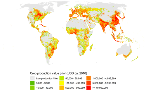
where Cropval_i is the value of total crop production in pixel i, prod_i,j is the production of crop j in pixel i and price_j is the price of crop j. A map of the global gridded crop production value as a prior is shown in Fig. 1.

Figure 1 The assembled crop production value used as a prior in the cross-entropy model (FAO, 2016; Yu et al., 2020).

2.1.2 Livestock production

Livestock accounts for an estimated 40 % of the global value of agriculture output and plays an important role in ensuring the livelihood and food security of over one-sixth of the world's population (FAO, 2018). However, it is still under rapid expansion as the global demand for animal-sourced products such as meat, milk, eggs and hides continues to grow (Herrero and Thornton, 2013). While species and quantities of livestock raised vary among regions and husbandry farmers, there are five primary species – cattle, sheep, goats, pigs, and chicken – that prevail worldwide and provide essential products for human consumption.

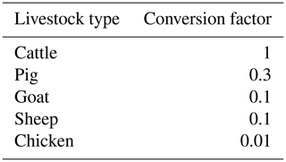
We calculate the prior for the component of livestock production in gridded AgGDP based on the distribution maps of the above five primary species from the Gridded Livestock of the World (Robinson et al., 2014; Gilbert et al., 2018) and FAOSTAT's value of production of livestock products (including meat, milk, eggs, honey and wool) (FAO, 2020). Due to data limitations, distribution maps for other animals such as ducks, horses, camels and bees are not available. However, the FAOSTAT livestock production values include a more comprehensive list of animals and their products. By distributing FAOSTAT values to grids in proportion to the five primary livestock species, we assume that other animals included in FAOSTAT have a similar spatial distribution to the five primary livestock species. This assumption is generally valid but may not be accurate in special areas such as deserts, where camels are an important source of livestock products. To facilitate comparison, the animal-specific density numbers are converted to one animal type by using International Livestock Units as conversion factors (Eurostat, 2018) as shown in Table 1. The conversion factors reflect biomass differences between different animals.³ Then the densities of the animal-equivalent values are multiplied by the total area of each 5 arcmin pixel to get the count of animals per grid, which is used to calculate the share of animal counts and is then multiplied by the FAOSTAT value of production to obtain the livestock production prior for each pixel.

$$\begin{array}{}\text{(3)}& {\mathrm{lsval}}_i={\mathrm{lsval}}_x{\displaystyle \frac{{\mathrm{lsnum}}_i}{{\mathrm{\Sigma }}_X{\mathrm{lsnum}}_i}},\forall i\in X,\end{array}$$

where lsval_i is the total value of livestock production in pixel i, lsval_x is the value of livestock production (meat, milk, eggs, honey and wool) that is reported at the national level, lsnum_i is the total number of equivalent animals in pixel i and X is a set including all pixels that fall within the boundary of a nation.

A map of global gridded livestock production value as a prior is shown in Fig. 2.

Table 1 Conversion factors for different livestock types. Source: Eurostat (2018).

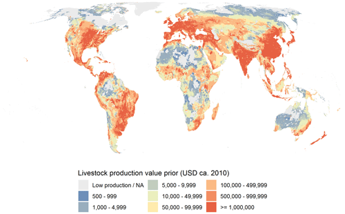
Figure 2 The assembled livestock production value used as a prior in the cross-entropy model. Sources: Robinson et al. (2014); Gilbert et al. (2018); Eurostat (2018).

2.1.3 Forestry production and hunting

People have utilized forest resources for a long time throughout history for their livelihood and various other purposes (Hossain et al., 2008). To date, over a billion people still rely on forest resources for food security and income generation to some extent (FAO, 2018). In the world’s least-developed regions, 34 countries depend on fuel wood to provide more than 70 % of energy, of which 13 nations require 90 % of energy (FAO, 2018).

The contribution of forest production to AgGDP can be classified into two broad types: wood (logging) products and non-wood forest products. Wood (logging) products are the most-exploited commodities in the forestry sector. The trees are harvested for fuel wood and industrial roundwood, which is processed into a variety of products, including lumber, plywood, furniture and paper products. Non-wood forest products are defined by the FAO.⁴ It is estimated that millions of households around the world depend on non-wood forest products for their livelihood. Some 80 % of people in the developing world use these products in their everyday lives (Sorrenti, 2016).

For a complete assessment of forest production priors, this study takes both wood and non-wood products into consideration. The gridded non-wood forest products dataset used in this study was jointly developed by Resources for the Future and the World Bank (Siikamäki et al., 2015) through an approach of meta-regression modeling, which integrates over 100 estimates at various locations from a literature review and multifold information on ecological and socioeconomic factors. The value of non-wood forest products is resampled to the 5 arcmin grid cell size and converted to 2010 USD for consistency with other AgGDP components. As part of non-timber products, we include hunting with an even distribution across units and time given the lack of information.

The value of wood products prior per pixel is calculated based on forest loss from year 2010 to year 2011 excluding loss due to fire, with an assumption that the forests were mainly cut down for timber production. The Moderate Resolution Imaging Spectroradiometer (MODIS) Land Cover map (Friedl et al., 2010) for year 2011 is overlaid on top of that for year 2010 to detect the area that has changed from forest to non-forest.⁵ However, forest loss due to fire needs to be removed because it does not result in timber production in most cases.⁶ Thus, fire information for year 2010 is obtained from the NASA Fire Information for Resource Management System (FIRMS) (NASA, 2018), and areas that experienced forest fires are eliminated. After the identification of the forest area change in each pixel, the value of wood production at the national level is taken from an FAO-led project (Lebedys and Li, 2014) and proportionally disaggregated to arrive at a pixel-wise value of wood products as follows:

$$\begin{array}{}\text{(4)}& \begin{array}{rl}{\mathrm{Woodval}}_i& =({\mathrm{forestval}}_x-{\mathrm{nonwoodval}}_x)\\ & {\displaystyle \frac{{\mathrm{forestloss}}_i}{{\mathrm{\Sigma }}_X{\mathrm{forestloss}}_i}},\forall i\in X,\end{array}\end{array}$$

where Woodval_i is the value of wood products in pixel i, forestval_x is the value of forest products reported at the national level, nonwoodval_x is the value of non-wood products at the national level which is derived from Siikamäki et al. (2015), forestloss_i is the area of forest loss excluding loss to fire in pixel i and X is a set including all pixels that fall within the boundary of a nation.

In our analysis of the forestry sector GDP, we have utilized the estimates provided by Lebedys and Li (2014) as the best available source. However, it should be noted that these estimates primarily capture activities within the formal forestry sector and do not take into account the value added generated by informal activities such as wood fuel production and non-wood forest products. To account for non-timber forest products, we have utilized the estimates provided by Siikamäki et al. (2015). Despite these efforts, it is acknowledged that the current analysis may still underestimate the forestry sector GDP due to the lack of reliable data on fuel wood production, which could account for half of global wood harvests (Ghazoul and Evans, 2004). This is a common issue as fuel wood values are often not properly captured in official statistics, as they are often collected for subsistence or sold in remote rural areas in many countries (Lebedys and Li, 2014). In future research, we intend to make efforts to acquire more reliable data on fuel wood production to improve the accuracy of our estimates of the forestry sector GDP.

A map of global gridded wood forest production value as a prior is shown in Fig. 3.

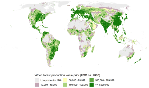
Figure 3 The assembled wood forest production value used as a prior in the cross-entropy model (Friedl et al., 2010; Siikamäki et al., 2015; NASA, 2018).

2.1.4 Fishery production

Fish makes up approximately 17 % of animal-sourced protein in the human diet worldwide (Mathiesen, 2018). The fishery industry supports the livelihood of 12 % of the world's population by creating 200 million jobs along its value chain. In the global trade system, USD 80 billion worth of fish is exported from developing countries, and it plays a crucial role in promoting local economic development (Kelleher et al., 2009).

We estimate both freshwater inland fishery and marine production values using the FISHSTAT (FAO, 2009) data with a classification based on the fish production categories. The inland fishery production value is the result of disaggregating corresponding country-level statistics in proportion to areas of inland water bodies in the 5 arcmin pixel. This is a simplified assumption and may cause overestimation in places where there are inland water bodies but not many fishery activities going on. The distribution of inland water bodies is obtained from the ESA-CCI (Lamarche et al., 2017). Thus, the value of inland fishing production in each grid is calculated as follows:

$$\begin{array}{}\text{(5)}& {\mathrm{fishval}}_i={\mathrm{freshval}}_x{\displaystyle \frac{{\mathrm{waterbody}}_i}{{\mathrm{\Sigma }}_X{\mathrm{waterbody}}_i}},\forall i\in X,\end{array}$$

where fishval_i is the value of fishery production in pixel i, freshval_x is the value of fresh fish production at the national level which is aggregated from FISHSTAT, waterbody_i is the area of water bodies in pixel i and X is a set including all pixels i that fall within the boundary of a nation x.

The value of marine fishery production is determined by its proximity to fish landing ports and a composite indicator that equally weighs the number of vessel visits and the total holding capacity of the fishing vessels. We use the port database from the World Port Index (National Geospatial-Intelligence Agency, 2019) and the number of port visits with a vessel hold of fishing vessels from Hosch et al. (2019) to create a composite variable as the prior based on the sum (for each port) of the number of visits (each event in the database) and the total vessel hold at the port. The geographic coverage of the ports is calculated for each port using the minimum port distance provided in Hosch et al. (2019). Any distances greater than 150 km were considered to be 150 km in this analysis. The value of marine fishing production in each grid is calculated as follows:

$$\begin{array}{}\text{(6)}& {\mathrm{marineval}}_i={\mathrm{marineval}}_x{\displaystyle \frac{{\mathrm{portindex}}_i}{{\mathrm{\Sigma }}_X{\mathrm{portindex}}_i}},\forall i\in X,\end{array}$$

where marineval_i is the value of fishery production in pixel i, portindex_i is an equally weighted composite index of the number of visits and the total vessel hold in pixel i and X is a set including all pixels i that fall within the boundary of a nation x.

A map of global gridded fishery production value as a prior is shown in Fig. 4.

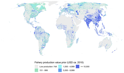
Figure 4 The assembled fishery production value used as a prior in the cross-entropy model (FAO, 2009; Lamarche et al., 2017; Hosch et al., 2019; National Geospatial-Intelligence Agency, 2019).

2.2 AgGDP statistics and linked grids

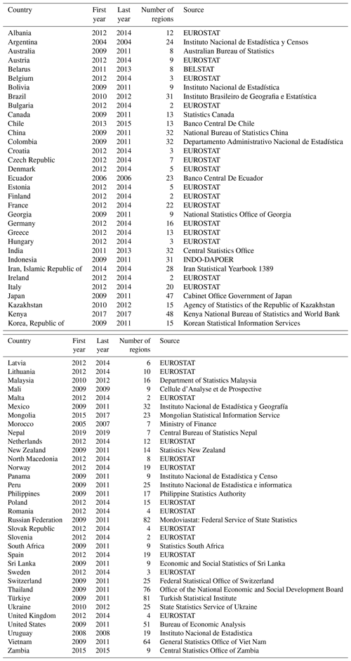
Substantial efforts have been made to collect and organize national and subnational statistics from a variety of sources, including national ministries and reports. However, not every country publishes its AgGDP figures at the subnational (regional) level, and there exist different methods of regionalization, including top-down, bottom-up and mixed methods (Eurostat, 2013).⁷ Our database has 68 countries that have subnational AgGDP data, expressed in varying domestic currencies and for different years. The typical administrative level is at the state or provincial level. Table  lists these countries and descriptive statistics, including the temporal coverage and the number of subnational regions at an administrative geographic level, including the NUTS level.⁸

To overcome discrepancies in temporal coverage and currency terms (constant and current) and to keep the data consistent and comparable for countries across the world, shares from subnational statistics are calculated and then applied to a national total to derive a calibrated number at the subnational level. The national totals are obtained from the publicly available World Development Indicators (WDIs) (World Bank, 2019) and averaged over 3 years around 2010. For a few countries that do not report their national AgGDP in the WDI database, sums of all AgGDP components are used as proxies.

The World Bank compiles these national accounts data following the International Standard Industrial Classification (ISIC) divisions 1–3 that include agriculture, forestry and fishing. Given the challenges of compiling national accounts data across the world, limitations include the exclusion of unreported economic activity in the informal or secondary economy. In particular, agricultural output in developing countries may not be reported due to issues such as natural losses or self-consumption and may not be exchanged for money. Despite best efforts, agricultural production may be estimated indirectly, leading to approximations that are different than the true values.⁹

The calibrated statistics are then linked to grids through a shapefile of the Global Administrative Unit Layers (GAUL) that maintains global geographic layers with a consistent and comprehensively unified coding system (FAO, 2015). Then, we overlay the GAUL administrative boundaries on the grid network to assign the corresponding codes of the administrative units to each grid.¹⁰ For areas where subnational AgGDPs have different administrative areas than GAUL, the GAUL areas are merged or split to match the subnational AgGDP areas.

2.3 Spatial allocation model

After constructing all the components, we define a spatial allocation model in a cross-entropy framework following You et al. (2014) to allocate administrative statistics to 5 arcmin pixels.¹¹ National and subnational AgGDP values are used as a constraint, while the distribution of crop, livestock, fishery and forestry production (hunting is included in non-timber products of forestry) is used to create priors for estimating pixel-level AgGDP. In actuality, the priors that we have constructed do not encompass all elements of AgGDP, and the national and subnational AgGDP statistics include a broader range of production values. However, the priors account for most variation between pixels, and thus their shares can serve as appropriate proxies in the AgGDP disaggregation model. Lastly, measurement units are unified using deflators and exchange rates.¹²

The first step is to transform all real-value parameters into corresponding probabilities. Let S_i be the share of the total AgGDP allocated to pixel i within a country x. AgGDP_i,x is the AgGDP allocated to pixel i in country x, and X is a set including all pixels that fall within the boundary of a nation. Therefore,

$$\begin{array}{}\text{(7)}& S_i={\displaystyle \frac{{\mathrm{AgGDP}}_{i,x}}{{\mathrm{\Sigma }}_X{\mathrm{AgGDP}}_{i,x}}},\forall i\in X.\end{array}$$

Let PreAgGDP_i be the pre-prior allocation of the AgGDP share from our best estimate. The first approximation can be done by summing all five calculated pixel-level components of AgGDP:

$$\begin{array}{}\text{(8)}& \begin{array}{rl}{\mathrm{PreAgGDP}}_i& ={\mathrm{Crop}}_i+{\mathrm{Livestock}}_i+{\mathrm{Forestry}}_i\\ & +{\mathrm{Fishing}}_i+{\mathrm{Hunting}}_i,\end{array}\end{array}$$

where we assume hunting occurs in areas with equal probability.

Theoretically, the sum of these components should be close to the official values obtained from the World Development Indicators. However, it should be noted that due to limitations in the available data, we have some components in output values (crop, livestock and fishery), whereas others in value added are added (forestry and hunting). This may result in discrepancies and inconsistencies. Overall, we make sure that the official AgGDP values are guaranteed to be no less than the sum of all five components of AgGDP.

$$\begin{array}{}\text{(9)}& {\mathrm{AgGDP}}_x={\mathrm{\Sigma }}_{i\in x}{\mathrm{PreAgGDP}}_i\end{array}$$

Then we rescale the prior AgGDP to be consistent with the official AgGDP value:

$$\begin{array}{}\text{(10)}& {\mathrm{PriorAgGDP}}_i={\displaystyle \frac{{\mathrm{PreAgGDP}}_i{\mathrm{AgGDP}}_x}{{\mathrm{\Sigma }}_i{\mathrm{PreAgGDP}}_x}}.\end{array}$$

Then we calculate the prior for S_i as a probability by normalizing PriorAgGDP:

$$\begin{array}{}\text{(11)}& {\mathrm{PreAlloc}}_i={\displaystyle \frac{{\mathrm{PriorAgGDP}}_{i,x}}{{\mathrm{\Sigma }}_{i\in X}{\mathrm{PriorAgGDP}}_i}}.\end{array}$$

Finally, we formulate a cross-entropy model in the following mathematical optimization framework:

$$\begin{array}{}\text{(12)}& \text{MIN CE}\left(S_i\right)={\mathrm{\Sigma }}_i{S}_i\log \left(S_i\right)-{\mathrm{\Sigma }}_i{S}_i\log \left({\mathrm{PreAlloc}}_i\right),\end{array}$$

subject to the following three conditions:

$$\begin{array}{}\text{(13)}& {\displaystyle }{\mathrm{\Sigma }}_i{S}_i=\mathrm{1},\text{(14)}& {\displaystyle }{\mathrm{\Sigma }}_{i\in k}\left(\mathrm{\Sigma }\mathrm{AgGDP}\right)S_i={\mathrm{SubAgGDP}}_k\forall k,\text{(15)}& {\displaystyle }\mathrm{0}\le S_i\le \mathrm{1}\forall i,\end{array}$$

where i: i=1, 2, 3, … are pixel identifiers within the allocation unit (e.g., Brazil) and k: k=1, 2, 3, … are identifiers for subnational geopolitical units (e.g., a state) where AgGDP values (SubAgGDP_k) are available. The objective function is defined as the cross-entropy of AgGDP shares and their priors. The first constraint (Eq. 13) is the pycnophylactic or volume-preserving constraint (e.g., Tobler, 1979) that ensures the sum of all allocated AgGDP values is equal to the total AgGDP of the country. The next Eq. (14) sets the sum of all allocated AgGDP values within those subnational units with available data to be equal to the corresponding subnational AgGDP values. The last Eq. (15) is a natural constraint for the share of AgGDP to be between 0 and 1, which is also the probability in the cross-entropy model. The modeling framework is flexible in that more constraints can be added if more data are available and/or more reasonable assumptions about how AgGDP should be spatially disaggregated are discovered.¹³ Last but not least, we multiply the total regional AgGDP by the probability in the cross-entropy model to derive the final pixel-level AgGDP:

$$\begin{array}{}\text{(16)}& {\mathrm{AgGDP}}_i={\mathrm{\Sigma }}_i{\mathrm{AgGDP}}_x{S}_i.\end{array}$$

3 Results, uncertainty and validation

3.1 Results

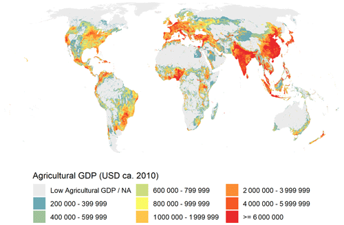
Figure 5 illustrates the result of the cross-entropy model in a global map of the gridded AgGDP. The global gridded AgGDP for the year 2010 in 2010 USD is in gridded (raster) format at a resolution of 5 arcmin, which approximates to 10 km.¹⁴ The spatial extent and quantity distribution of AgGDP over the world are in agreement with general knowledge of agricultural technology adoption and suitability, with well-known agricultural nations such as India, China and the United States standing out as regions with relatively high AgGDP compared with many other areas of the world. A number of European countries also exhibit high AgGDP values, which is likely due to the benefit of adopting mechanized farming and technological facilitation, considering that the shares of agricultural land and agrarian population are relatively low in these well-developed places. Countries in sub-Saharan Africa remain low in agricultural production, as indicated by low-value pixels sparsely spreading over the continent. Within the continent, agricultural production activities primarily take place in geographic areas with suitability and access to markets (e.g., land cultivation; see Berg et al., 2018).

Figure 5 Global gridded AgGDP circa 2010 from the cross-entropy model in 2010 USD.

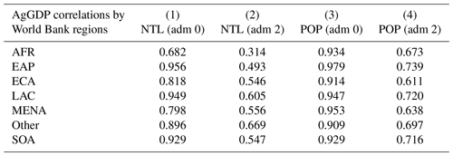
We examine the correlation of the AgGDP dataset with two commonly used global datasets to proxy economic activity: nighttime lights and population. Nighttime light data are commonly used in the estimation of local human development and economic activity (e.g., Ghosh et al., 2010; Henderson et al., 2012; Bundervoet et al., 2015; Kummu et al., 2018; Bruederle and Hodler, 2018). We use the sum of the radiance-calibrated data for 2010 from the F16 satellite to quantify the correlation between AgGDP and nighttime lights by geographic regions of the world defined by the World Bank.¹⁵ We use rural population derived from Center for International Earth Science Information Network – CIESIN – Columbia University (2017) following methods in Thomas et al. (2019). We use country-level data from the World Bank World Development Indicators (World Bank, 2019). We find that the correlation of AgGDP with night light varies across world regions, with sub-Saharan Africa and the Other region showing lower correlation values (Table 2). Most World Bank regions have similar patterns of correlation with nighttime lights across the measures of AgGDP and population. Likewise, World Bank income groups show similar patterns across the measures, with the lower-middle and upper-middle income groups having higher correlations than the low- and high-income groups. However, notable differences in the correlations exist between geographic levels. The mean correlation of AgGDP with nighttime lights (NTL) and population (pop) derived from administrative level-2 data is lower than the national level, which presents evidence of new information from the AgGDP dataset.

Table 2 Spearman correlation of AgGDP with nighttime lights at the Admin 0 level (1) and Admin 2 level (2) as well as the rural populations at the Admin 0 level (3) and Admin 2 level (4), grouped by World Bank region where AFR is sub-Saharan Africa, EAP is East Asia and the Pacific, ECA is eastern Europe and central Asia, LAC is Latin America, MENA is the Middle East and North Africa, SOA is South Asia, and Other is the category for the remaining countries (NOAA, 2011; World Bank, 2019).

Furthermore, limitations exist with these commonly used datasets for applications of AgGDP. For nighttime lights, Li et al. (2020) provide a cautionary note about rural applications where the presence of agricultural activities typically takes place. A population model assumes proportional activity to population by strata (e.g., rural), which does not account for the type of rural of agricultural activity, and the model requires a standard definition of rural, which can pose challenges in global applications (e.g., stylized facts in the urban and development economics literature Roberts et al., 2017). Notably, the rural population dataset also has variation in the geographic level of the input information, which informs the estimates of population models and currency across the world, especially when dependent on the frequency of production and the availability of a population census. Also, the AgGDP dataset may attenuate modeling concerns of endogeneity when using AgGDP along with population or nighttime lights.

3.2 Fitness for use and uncertainty

We provide descriptive statistics of the data and modeling from a fitness-for-use perspective (e.g., Leyk et al., 2019). The data are most appropriate for applications at global, continental and regional scales (You and Wood, 2006). However, decisions regarding the use of the data at smaller spatial extents should be made with caution and with consideration of the underlying assumptions and characteristics of the area in question. Users should take into account factors such as area of the grid cell of AgGDP, the number of subdivisions of AgGDP from the political area (e.g., country) and assumptions in the priors (e.g., see shares of priors in Table B8). When input data contain multiple observations, the AgGDP dataset may still be suitable for use, as it is already standardized in grid cells, which may facilitate integration with other data. As the spatial refinement of ancillary data advances along with greater currency, coverage and representativeness, we expect validation possibilities to increase and inform a better understanding of the uncertainty and the associated fitness for use. Also, we intend to improve spatial and temporal coverage when this is feasible.

The process of disaggregating the data from the source level to the target level does impose spatial relationships and is prone to error (Li et al., 2007) and the modifiable areal unit problem (MAUP) (Openshaw, 1981). In previous work, our team conducted sensitivity analyses and examined the consequences of methodological-data choices involved in a cross-entropy model to disaggregate crop production statistics (Joglekar et al., 2019). These analyses included eight scenarios that varied in allocation methods, data groupings, input variables and different levels of statistics. The analysis indicated that allocation results are most dependent on the degree of disaggregation and the quality of the underlying national and subnational production statistics. Therefore, we provide more discussion in Sect. 3.2.1 (Regional accounts). Additionally, the results are moderately sensitive to allocation methods. We previously compared three models for the case of Brazil (Thomas et al., 2019) and found that cross-entropy is the most appropriate method for the global study, with relatively high accuracy and flexible data requirements when compared with either the spatial regression or rural population methods. Interested readers may find more details in the Brazil paper. Lastly, the results are somewhat sensitive to the groupings and formats of input components that serve as priors, which we discuss in Sect. 3.2.2 (Components).

3.2.1 Regional accounts

The measurement of GDP is challenging (Angrist et al., 2021), especially agricultural production (Carletto et al., 2015). The level of uncertainty associated with these results includes the thematic, spatial and temporal accuracies. We collected regional accounts by sector from various sources into a global database. The data are not balanced over time or at the geographic level. The variation in the reference year of the regional accounts data influences the temporal balance of the database. This mismatch can influence the regional distribution of the AgGDP that may be different than the target reference year of 2010. Given climate¹⁶ and specifically rainfall are important inputs to crop and livestock production and may contribute to variation across years (Stanimirova et al., 2019; Zhang et al., 2020), we attempt to reduce this source of error by averaging over multiple years when data are available, which is a similar approach to You et al. (2014). However, this does not eliminate this mismatch. The availability of data varies when grouped by World Bank income (low or lower-middle, upper-middle and high income). The average absolute temporal difference (ATD) defined as the mean difference in years between the reference regional accounts and the target year (2010) is higher in the low and lower-middle income groups. Likewise, the mean deviation of the share of AgGDP by country over the year(s) is larger in the low- or lower-middle income groups compared to the high-income one.

The global regional accounts database includes national and subnational units at various administrative levels.¹⁷ Following Robinson et al. (2014) in their assessment of Gridded Livestock of the World (GLW) 2.0, we summarize the average spatial resolution (ASR) of the input regional data, which is the square root of the land area divided by the number of administrative units (see Fig. 6). We find that on average the ASR value increases from high- to low-income groups based on World Bank 2010 classifications. Following Yu et al. (2020), we suggest that users can view the ASR map as an indicator of uncertainty level since the model is proven most dependent on the ASR of statistics. A larger ASR represents more sparsity of input statistics and more uncertainty of the gridded results.

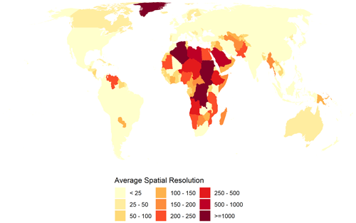
Figure 6 The average spatial resolution of the regional accounts data by country (World Bank, 2019). See also the various sources in the Appendix.

3.2.2 Components

Another source of uncertainty is the indirect temporal inaccuracy propagated from the input datasets of the components, which are modeled. We discuss all five components of AgGDP: crop, livestock, forest, fish and hunting. The SPAM model (You et al., 2014) is a result of several gridded modeled datasets, including rural population density from the Global Rural-Urban Mapping Project (GRUMP) Alpha version (Balk et al., 2006). Likewise, the Gridded Livestock of the World v2.0 includes rural population density in 2006 (GRUMP) along with other predictors such as precipitation (Hijmans et al., 2005) and a modeled travel time to places with 50 000 inhabitants circa 2000 (Nelson, 2008). Anderson et al. (2015) find variation in their examination of global data products of cropping system models. For livestock, we transform the five major livestock types into international values from livestock products (i.e., meat, milk, eggs, honey and wool). The forest (non-wood products, wood products) components rely on a remote-sensing model to estimate forest loss. With regards to the non-timber values, limitations from the sources present two challenges. The estimates use simple averages from the literature that accordingly assume a property of uniformity in the value of a hectare of forest to be similar across the world, and the sample of forests with the literature drawn for the study is representative of the world (Siikamäki et al., 2015). The fishing model relies on the proximity and association with ports or water bodies.¹⁸ Finally, since we do not incorporate any information on hunting, the result is an even distribution across units and time.

Another source of uncertainty is the geographic distribution of the components. Ideally, we would use subnational prices; however, this was not feasible. So, the results do not reflect this occurrence, and there is a potential misrepresentation of administrative units with high variation of prices due to the heterogeneity of distinct urban and rural areas.

3.3 Validation

A true validation of the predictive accuracy of this model involves data collection and construction of agricultural gross regional products in different pixels and testing those independent observations against the predicted values. The regional production data are, however, generally constructed at the administrative level rather than the pixels, so validation would have to be done on an aggregation of model predictions. Few countries provide the required data to assess the prediction accuracy to examine the internal validation of the disaggregation efficiency, and the data collection would be extremely costly and time-consuming. An evaluation of prediction accuracy requires input data at a local level, which is not available for all countries.

Multiple geographic levels of AgGDP exist for the case of Brazil, where we conducted a pilot study and examined the validity of various methods to disaggregate AgGDP spatially, including cross-entropy, a rural-population-based model and spatial regression (see Thomas et al., 2019). Administrative divisions of Brazil consist of 558 microregions, which are further divided into 5564 municipios. We had AgGDP data at both the microregion and municipio levels. In order to test the methods, we only used statistics for the 558 microregions and allocated them to gridded pixels. Then we aggregated estimated results at the pixel level to 5564 municipios and compared them with ground-truth data. Results showed that the correlation between the predictions and actual values at the municipio level was 0.91 for the cross-entropy model. Mean absolute deviation (MAD) and root mean square error (RMSE) were 8249 and 18 347, respectively, while the average of the municipio-level true values was 28 739 (BRL 1.000). The performance of the spatial regression model was slightly better than the cross-entropy model, but it can hardly generalize to the global work since for many countries we only have one number at the national level and do not have enough degrees of freedom for the regression model. The naïve rural population model had a correlation value of 0.81 between the predictions and actual values at the municipio level, and MAD and RMSE were 28 744 and 25 397, respectively. The cross-entropy model was proven to have relatively high accuracy compared to the naïve model and better flexibility to accommodate data scarcity in certain countries and thus was chosen as the model for the global AgGDP dataset.

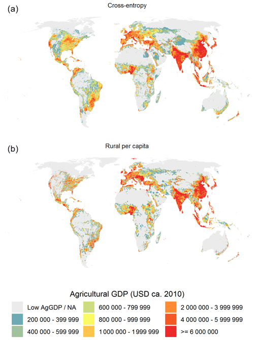
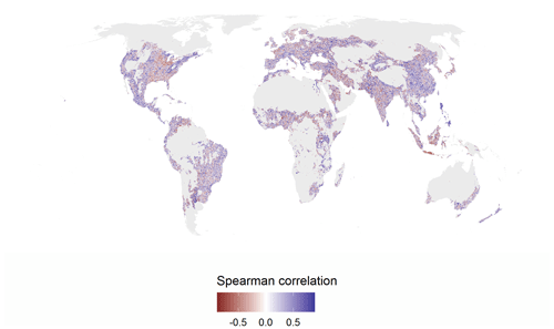
At the global scale, since we do not have AgGDP statistics at lower administrative levels consistently, we are not able to validate estimated results by aggregating to different geographic levels like the Brazil case. In addition, due to the volume-preserving pycnophylactic property of the cross-entropy model that utilizes all available data from mixed levels and ensures that the aggregated values conform to all the original values, we do not have extra data for validation. All available data have been internalized by the model to improve estimation results and thus cannot serve as external validation. Nevertheless, we compare the results from the global cross-entropy model to that from a rural population-based model at the grid level and examined their correlation, which is a similar assessment to You et al. (2014) (as mentioned, a spatial regression model at the global scale is not feasible due to insufficient degrees of freedom). We construct a proportional allocation model using rural population count following the method in Thomas et al. (2019) for the case of Brazil. We use the 2010 Gridded Population of the World version 4 from Center for International Earth Science Information Network – CIESIN – Columbia University (2017) adjusted to the United Nation's World Population Prospects followed by including the rural area defined by the Global Human Settlement grid for 2015, i.e., “Rural cluster”, “Low Density Rural grid cell” or “Very low density rural grid cell” (Pesaresi and Freire, 2019). We disaggregate national or subnational AgGDP statistics to grids in proportion to their rural population, with each rural individual receiving an equal portion of the AgGDP. Figure 7 shows results of the rural per capita model and the cross-entropy model together. We can test the similarity of the two global maps. Following Levine et al. (2009), we assume a normal distribution over the 2 million land pixels and perform a pairwise Student's t test to test the null hypothesis that both maps were identical. This test allows us to examine whether the mean difference in the corresponding pixel value from one map to another was greater than would be expected by chance alone. The t-test statistic tells us that we cannot reject the null hypothesis, which provides some evidence of similarity between the two models using all the global pixels. However, at a granular spatial level, Fig. 8 shows variation in local correlation across the world. We use a Spearman correlation for a 3×3 window of pixels with a focus on AgGDP areas with values above 200 000, excluding the Low Agricultural GDP/NA category where the measurement of rural population and AgGDP may have discontinuity due to modeling inaccuracies. The lack of similarity illustrates the difference in the spatial distribution of agricultural production systems that are not directly correlated with population density within a geographic level. At the granular spatial level, populated places and agricultural land use are different locations to allocate AgGDP. The rural per capita model is dependent on the input geographic level, where average spatial resolution may vary, as well as on the quality and resolution of ancillary data like built-up areas (e.g., Rubinyi et al., 2021).

Figure 7 A panel map of gridded AgGDP circa 2010 from the cross-entropy model (a) and from the rural per capita population model (b) Authors' calculation.

Figure 8 Spearman correlation in areas of AgGDP above or equal to 200 000 in the cross-entropy and rural per capita models.

4 Illustration of use: drought risk and water scarcity

Following previous global studies (e.g., Blankespoor et al., 2017; Rentschler et al., 2022), we present an application of the population exposed to a natural hazard. Specifically, we investigate the spatial distribution of population and agricultural activity with regards to drought and water scarcity. These two indicators provide an illustrative example of different linkages to agricultural production. Drought highlights the linkages to crops and livestock, whereas water scarcity focuses attention on the distribution of a population. The global population estimates for the year 2010 are from the WorldPop and Center for International Earth Science Information Network (CIESIN), Columbia University (2018).¹⁹ For a drought index, we calculate the Standardized Precipitation Evapotranspiration Index (SPEI) (Vicente-Serrano et al., 2010), which measures the difference between observed precipitation and estimated potential evapotranspiration with a 3-month interval using the base climatology of 1980 to 2019, which is implemented in R (Beguería and Vicente-Serrano, 2017) using climate data from Harris et al. (2020). Extra-dry years are defined as the number of years that are less than or equal to −2.0 during the period from 2000 to 2009. Figure A1 shows the results of the SPEI. The Water Crowding Index (WCI) is a measure of water scarcity considering the local population as the annual water availability per capita (Falkenmark, 1986, 2013). Veldkamp et al. (2015) model the global WCI with return periods. We take the mean of any pixels of the ensemble WCI with a 10-year return period within an AgGDP pixel. Following the literature (e.g., Arnell, 2003; Alcamo et al., 2007; Kummu et al., 2010; Veldkamp et al., 2015), we categorize the WCI into four categories: absolute is less than 500 m³ per capita per year, severe is less than or equal to 1000 m³ per capita per year, moderate is less than or equal to 1700 m³ per capita per year, and low is the remainder (Fig. A2). Then, we evaluate water shortage events using a threshold of 1700 m³ per capita per year with a return period of 10 years.

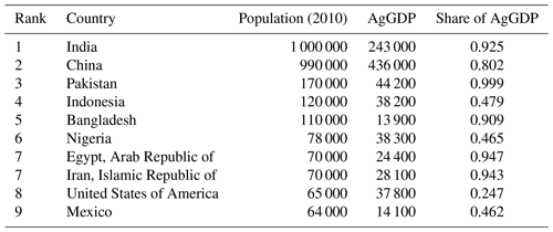
The exposure to drought is not uniform across the world. Across the world, the group of high-income countries has lower populations and AgGDP exposed to drought in each number of years with extremely dry conditions compared to the countries in other income categories (Fig. 9). Areas that are exposed to at least one extreme drought from 2000 to 2009 account for an estimated AgGDP of USD 432 billion and a population of 1.2 billion. The top 10 countries in total AgGDP exposure include the large economies in the agriculture sector such as China, India, the United States and the Russian Federation (Table B1). However, other countries have a high share of their AgGDP exposed to extreme drought (Table B5). The top 10 countries in 2010 population exposed to dry areas include countries with the largest economies in the agriculture sector as noted above, but the list includes countries such as the Democratic Republic of Congo, Tanzania and Uganda (Table B3).

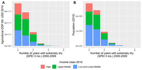
Figure 9 The total exposure of AgGDP (a) and population (b) aggregated from areas with at least one extreme drought from 2000 to 2009 measured by a 3-month SPEI (WorldPop and Center for International Earth Science Information Network (CIESIN), Columbia University, 2018; World Bank, 2019).

Across the world, high-income countries have lower populations and AgGDP in areas of absolute or severe categories of the Water Crowding Index compared to countries in other income categories (Fig. 10). The top 10 countries of AgGDP exposed to the Water Crowding Index include large economies in the agriculture sector such as China, India, Pakistan, Indonesia and Nigeria (Table B4). However, several countries have a high share of their AgGDP exposed to the Water Crowding Index (Table B2). The top 10 countries in 2010 population exposed to dry areas include countries with the largest economies in the agriculture sector as noted above, but the list includes countries such as Bangladesh, the Arab Republic of Egypt and Mexico (Table B6).

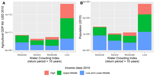
Figure 10 Total AgGDP (a) and population (b) by mean Water Crowding Index, where absolute is less than 500 m³ per capita per year, severe is less than or equal to 1000 m³ per capita per year, moderate is less than or equal to 1700 m³ per capita per year, and low is the remainder (Veldkamp et al., 2015; World Bank, 2019).

5 Data availability

These data are available at the World Bank's Development Data Hub under https://doi.org/10.57966/0j71-8d56 (IFPRI and World Bank, 2022).

6 Conclusions

A globally consistent dataset on local estimates of AgGDP could benefit research and policymaking in a wide range of areas related to nature conservation, economic development and disaster management. However, such data have been missing. In this paper, we made the first attempt to create a novel global dataset that disaggregates the national and regional accounts of the agriculture sector into 5 arcmin grids using cross-entropy optimization based on ancillary data of satellite-derived products. The gridded data format provides flexibility when the map is integrated with other data sources. It can be aggregated to various levels using administrative boundaries or other boundaries of interest, such as natural hazard zones. Since most interventions are geographically targeted, this dataset will provide important information on local variations in agricultural production and help identify places of policy interest. We illustrate the usage of this dataset through an exposure analysis of agriculture production to drought risk and water scarcity and examine uneven natural hazard exposure across the world with USD 432 billion of AgGDP and 1.2 billion people. With increasing frequency and severity of natural hazards such as floods, droughts and cyclones, socioeconomic estimates at the local level play an increasingly important role in informing the preparations of disaster response.

These data are the result of data collection and collaboration across multiple entities to ensure the most current and widest coverage. However, persistent challenges to data collection remain, including limited geographic levels and temporal lags with low frequencies. Also, the reference year and spatial resolution of the local AgGDP estimates are limited to the contemporaneous availability of the economic statistics and components such as the crop production model. We often have to consider the fitness for use while considering the accuracy; the model has a higher ASR in areas where we have few data. However, these same areas may benefit from the availability of these estimates to inform policy. Predictions are dependent on the availability and quality of the training data on which the model is based, and the modeling process is flexible to update individual countries as the data are available.

In the near future, we hope to update this dataset as the currency and number of countries with subnational data increase along with updated data for different agricultural components. We have learned that the main input for our crop component, SPAM, now includes data for 2017 in sub-Saharan Africa and is in the process of producing a global crop map for 2020. Additionally, the FAO livestock distribution maps for our livestock component have been updated to include a greater variety of animal types for the more recent year of 2015. We also intend to utilize annually updated satellite imagery from MODIS Land Cover and ESA-CCI in order to calculate more recent data for the forestry and fishery sectors. In future work, we will also make the necessary adjustments to include fuel wood production and exclude trees that are cut down for plantation replanting and not used for further timber production in the calculation of forestry sector GDP.

Appendix A: Figures

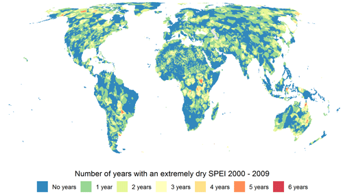
Figure A1 The number of years with at least one extreme drought from 2000 to 2009 measured by a 3-month SPEI (Harris et al., 2020; Beguería and Vicente-Serrano, 2017).

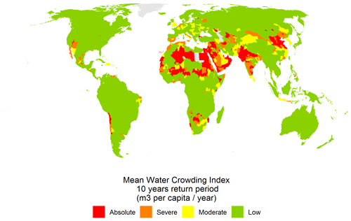
Figure A2 Water Scarcity Index categories with a return period of 10 years (Veldkamp et al., 2015).

Appendix B: Tables

Table B1 Top 10 countries with the largest total agricultural GDP (millions of USD) exposed to dry areas with shares of agricultural GDP and population (thousands).

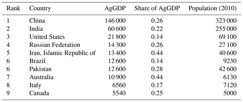
Table B2 Top 10 countries of the largest share of agricultural GDP exposed to dry areas with agricultural GDP (millions of USD) and population (thousands).

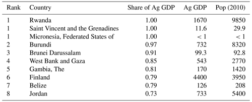
Table B3 Top 10 countries of 2010 population (thousands) exposed to dry areas with agricultural GDP (millions of USD) and share of agricultural GDP.

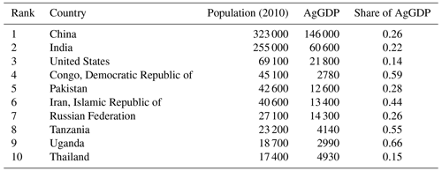
Table B4 Top 10 countries with the largest total agricultural GDP exposed to WCI areas with agricultural GDP (millions of USD) and population (thousands).

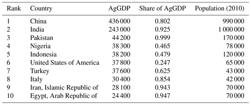
Table B5 Top 10 countries with the largest share of agricultural GDP in countries exposed to WCI areas with agricultural GDP (millions of USD) and population (thousands).

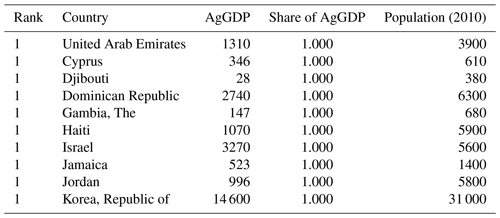
Additional countries exposed to WCI areas with a 1.00 share of AgGDP include the West Bank and Gaza, Cyprus, Kuwait, The Gambia, Qatar, and Hong Kong (SAR, China).

Table B6 Top 10 countries of 2010 population exposed to WCI areas with agricultural GDP (millions of USD) and population (thousands).

Table B7 Regional accounts descriptive statistics.

Table B8 Share of priors in territory.