Southern Europe and western Asian marine heatwaves (SEWA-MHWs): a dataset based on macroevents

Marine heatwaves (MHWs) induce significant impacts on marine ecosystems. There is a growing need for knowledge about extreme climate events to better inform decision-makers on future climate-related risks. Here we present a unique observational dataset of MHW macroevents and their characteristics over the southern Europe and western Asian (SEWA) basins, named the SEWA-MHW dataset (https://doi.org//10.5281/zenodo.7153255; Bonino et al., 2022). The SEWA-MHW dataset is derived from the European Space Agency Sea Surface Temperature Climate Change Initiative (ESA SST CCI) v2 dataset, and it covers the 1981–2016 period. The methodological framework used to build the SEWA-MHW dataset is the novelty of this work. First, the MHWs detected in each grid point of the ESA CCI SST dataset are relative to a time-varying baseline climatology. Since intrinsic fluctuation and anthropogenic warming are redefining the mean climate, the baseline considers both the trend and the time-varying seasonal cycle. Second, using a connected component analysis, MHWs connected in space and time are aggregated in order to obtain macroevents. Basically, a macroevent-based dataset is obtained from a grid cell-based dataset without losing high-resolution (i.e., grid cell) information. The SEWA-MHW dataset can be used for many scientific applications. For example, we identified phases of the well-known MHW of summer 2003, and taking advantage of statistical clustering methods, we clustered the largest macroevents in SEWA basins based on shared metrics and characteristics.

1 Introduction

Over the past few decades, anomalous prolonged events of warm sea surface water, known as marine heatwaves (MHWs), have developed globally, both in the open ocean and in coastal regions, leading to serious consequences for marine ecosystems. The ecosystems are very sensitive to abrupt temperature changes, and they can reach their “tipping point” (Lenton et al., 2008; Serrao-Neumann et al., 2016), which means entering into an unknown state which may be completely distant from the previous one. Increased ocean temperatures imply a large number of ecological repercussions, spanning from a coast-wide onset of toxic algae (McCabe et al., 2016; Ryan et al., 2017) to dramatic range shifts in species at all trophic levels (Cavole et al., 2016; Sanford et al., 2019). These adverse conditions during MHWs can lead to substantial economic losses for important fisheries and aquaculture industries (McCabe et al., 2016; Cavole et al., 2016; Frölicher, 2019).

Some relevant examples of unprecedented ocean temperature anomalies are the 2011 Australian marine heatwave in the eastern Indian Ocean (Pearce et al., 2011) and the persistent 2014–2016 Blob in the North Pacific (Di Lorenzo and Mantua, 2016). In the Mediterranean Sea, several works reported an anomalous warm sea surface temperature during the summer of 2003 (e.g., Olita et al., 2007; Marullo and Guarracino, 2003; Grazzini and Viterbo, 2003). Darmaraki et al. (2019) identified the MHWs of 2003, 2012, and 2015 as being the most severe basin-scale surface events during the 1982–2017 period. Marbà et al. (2015), focusing on impacts of these extreme events on Mediterranean biota, reported basin-scale MHWs during 1994 and 2009 and a regional MHW over the Adriatic, the Ionian, and parts of the Levantine basin during the 1998. Other studies on ecological impacts identified MHWs over the western Mediterranean Sea during 2008 (Cebrian et al., 2011) and 2006 (Kersting et al., 2013) and over Adriatic Sea during 2009 (Di Camillo et al., 2013). Very limited information is available for MHWs in the Black Sea and in the Caspian Sea (e.g., Mohamed et al., 2022). They are usually related to works in which MHWs are detected and studied at global scales, such as Holbrook et al. (2020) and Sen Gupta et al. (2020).

A basic definition of MHWs (i.e., IPCC SROCC; see Pörtner et al., 2019) states that they are extremely anomalous temperatures in the ocean. However, to compare events and study their impacts, they must also be identifiable, with clear start and end dates and measurable characteristics. Hobday et al. (2016) were the first to propose a definition for MHWs, according to which the temperature must be higher than a given percentile (e.g., 90th, which is relevant to a reference climatology) and must persist for at least 5 d. This definition has been widely adopted by the oceanographic community (e.g., Holbrook et al., 2019; Oliver et al., 2021; Smale et al., 2019). However, it is worth mentioning that this definition is characterized by flexibility in the choice of the setup parameters (such as the climatology and the percentile threshold), thus limiting comparability among studies.

Most of the research conducted in this emerging field exploits this definition to study extreme events at individual locations (i.e., grid cells). Nevertheless, the grid-cell-based MHW events are likely connected in time and in space and part of the same extreme macroevent. Very few studies put effort into defining macroevents. For example, Darmaraki et al. (2019) and Pastor and Khodayar (2022) define the spatiotemporal extent of the MHW when a minimum of 20 % and 5 % of the Mediterranean Basin is affected by grid-cell-based MHWs, respectively. Sen Gupta et al. (2020) used a semi-objective procedure to characterize and detect the most extreme MHW macroevents globally, and Woolway et al. (2021) used a connected component analysis to study extreme temperature macroevents in the Laurentian Great Lakes. More recently, Sun et al. (2022) tracked the evolution in time of constructed snapshots of spatially compact MHWs. Macroevent-based studies facilitate the investigation of MHW drivers (Sun et al., 2022), which are currently not well understood (Holbrook et al., 2020). Driving mechanisms, which are usually seasonal and location dependent, are related to oceanic and atmospheric forcing or a combination of both (e.g., Oliver et al., 2018, 2021; Holbrook et al., 2019; Frölicher and Laufkötter, 2018). Examples of key phenomena which cause these extreme temperatures are anomalous horizontal advection, anomalous heat fluxes, sea level pressure anomalies, reduced coastal upwelling, Ekman pumping, or the re-emergence of warm anomalies from the subsurface (Schlegel et al., 2021; Holbrook et al., 2019, 2020). The timescale of these relevant physical drivers and processes involved in MHW emergence spans from days (e.g., anomalous heat fluxes) and weeks (e.g., blocking systems and atmospheric teleconnections) to months (e.g., re-emergence of warm anomalies from the subsurface) and years (e.g., climate modes and oceanic teleconnections; e.g., Oliver et al., 2018, 2021).

Given the pronounced warming trend in recent years, Benthuysen et al. (2020) and Holbrook et al. (2020) suggest the need for a more comprehensive and consistent framework to report MHWs. To the best of our knowledge, there is no available MHW macroevent dataset in the literature. Even thought MHWs are derived from sea surface temperature, whose observations are available, the processing to detect MHWs is computational and/or time-demanding, especially for high-resolution SST data.

In short, the current state of knowledge about MHWs requires addressing the need for more comprehensive efforts to document and report these extreme events. The aim of this paper is to provide a unique dataset of MHW macroevents derived from the European Space Agency (ESA) Climate Change Initiative (CCI) Sea Surface Temperature (SST) v2 dataset. The dataset consists of a daily dataset of MHW macroevents and their characteristics over the southern Europe and western Asian (SEWA) basins, named the SEWA-MHW dataset. We have focused on SEWA basins because they represent a well-known hot spot region for climate change (Giorgi, 2006) and for this specific phenomenon in particular (Garrabou et al., 2009; Giorgi, 2006; Cramer et al., 2018; Pastor and Khodayar, 2022; Pastor et al., 2020; Garrabou et al., 2022; Ciappa, 2022). Marine heatwaves caused unprecedented biological impacts, especially in the Mediterranean Sea (Garrabou et al., 2022; Cramer et al., 2018; Marbà et al., 2015; Rivetti et al., 2014), which seriously affected the marine biodiversity (Juza et al., 2022). Moreover, the Mediterranean Sea is recognized as an exemplary model for assessing the ecological and biological impacts of climate change (Garrabou et al., 2022; Cramer et al., 2018).

We generated the SEWA-MHW dataset in a new, consistent framework. In brief, we detected MHWs relative to a time-varying baseline climatology in each grid point of the ESA CCI SST dataset, and then, using a connected component analysis, we aggregated the spatiotemporally connected MHWs in order to obtain macroevents.

This paper is organized as follows: in Sect. 2, we present the data used to produce the SEWA-MHW dataset and the studied area. In Sect. 3, we describe the methodological framework applied to obtain the dataset, and in Sect. 4 we offer an example of its scientific application. Section 5 reports the availability of codes and data used to build SEWA-MHW dataset. Our conclusions and outlook of the work are summarized in Sect. 6.

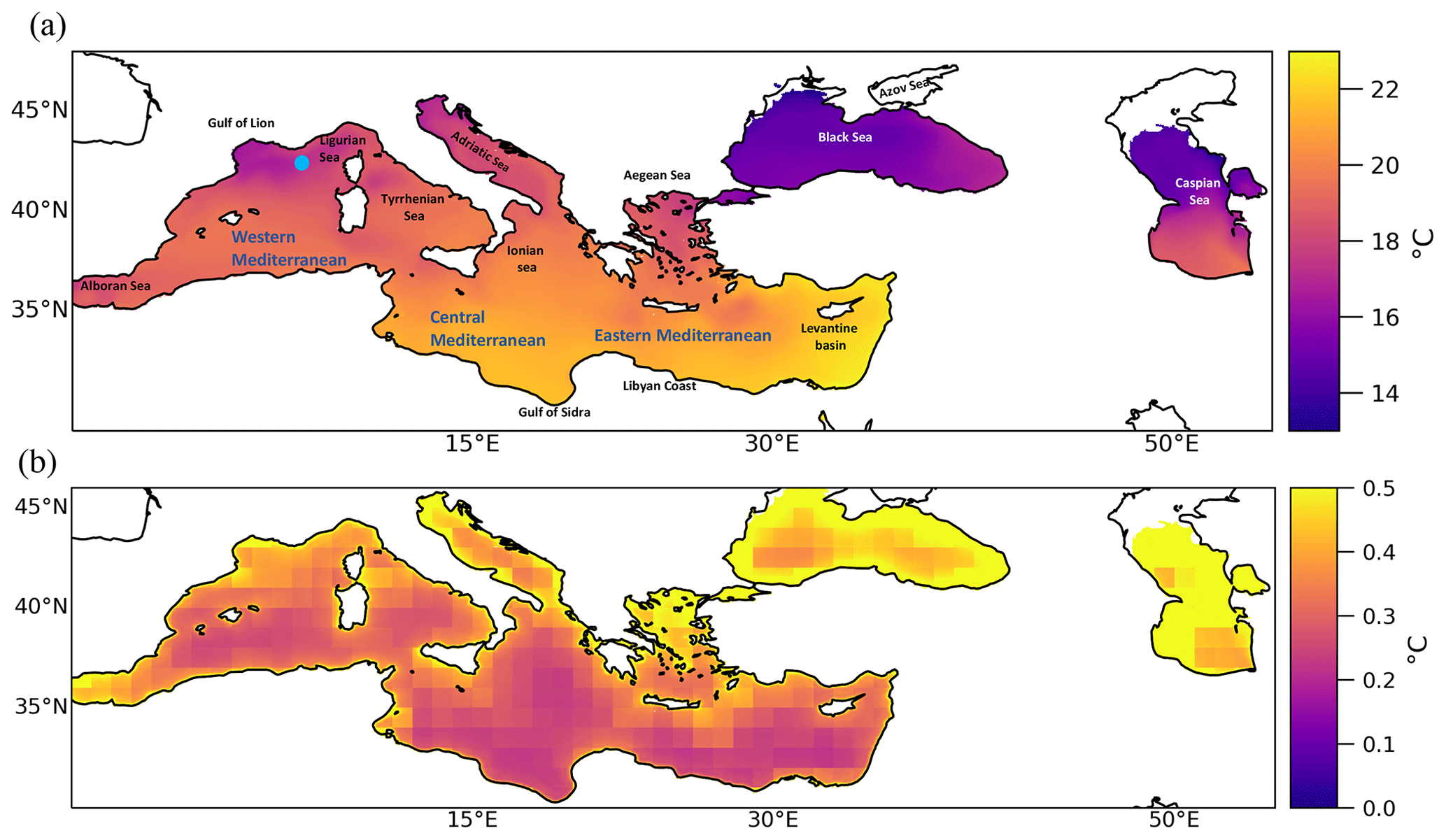
Figure 1 (a) Mean SST climatology detected by STL method with geographical names. The blue circle identifies the western Mediterranean location of the time series shown in Fig. 4. (b) The mean SST uncertainties during the studied period.

2 ESA SST CCI data and study area

To generate the SEWA-MHW dataset we used the European Space Agency (ESA) Climate Change Initiative (CCI) SST dataset v2.1 (hereinafter ESA CCI SST dataset). This dataset, available in the CEDA catalogue (https://catalogue.ceda.ac.uk/uuid/62c0f97b1eac4e0197a674870afe1ee6, last access: 14 March 2023), provides global daily satellite-based SST data covering the period from September 1981 to December 2016. A detailed overview of the processing updates for, and of the history behind, the ESA CCI SST dataset v2.1 is presented by Merchant et al. (2019). The ESA CCI SST v2.1 dataset is designed to provide a long-term, stable, low-bias climate data record derived from different infrared sensors, i.e., the Advanced Very High Resolution Radiometer (AVHRR), Advanced Along Track Scanning Radiometer ((A)ATSR), and Sea and Land Surface Temperature Radiometer (SLSTR) series of sensors (Merchant et al., 2019, 2014). In total, 17 missions from 1981 to 2016 contributed to the ESA CCI SST dataset (e.g., NOAA-6, ATSR-1, MetOp-A), and they are fully described in Merchant et al. (2019, see their Fig. 3). Different processing levels of the ESA CCI SST dataset are available, including the single-sensor data on the native swath grid (Level-2), uncollated single-sensor (Level-3U), collated multi-sensor (Level-3C) gridded data, and optimally interpolated (Level-4) multi-sensor data. Here, only the spatially complete Level-4 product (ESA CCI SST L4), obtained through the Operational Sea Surface Temperature and Ice Analysis (OSTIA) system (Donlon et al., 2012), is considered. This dataset consists of daily maps of average SST at 20 cm nominal depth with 0.05^∘ × 0.05^∘ of horizontal resolution, covering the period from September 1981 to December 2016. The ESA CCI SST L4 is adjusted to 20 cm depth in order to be comparable with drifter and historic bucket temperature measurements. Moreover, the dataset is also adjusted in time to address the SST diurnal heating allowed by the different overpass times of satellites that sample SST differentially. In particular, the temporal adjustment is applied as an estimate of the change in SST between the observation time and the nearest (10:30 or 22:30 UTC) local mean solar time, which is a good approximation of the SST daily mean (Morak-Bozzo et al., 2016). Observation data from 1991 onwards needed only a minimal adjustment, as these are always available for mid-morning satellite observations. Therefore, the diurnal heating is somehow taken into account in the ESA SST CCI L4 data processing. The data are adjusted in depth and in time to be more representative of the daily SST mean, which is the meaningful data frequency to define MHW events. The neglected diurnal warming in the SST dataset (e.g., SST provided at the foundation depth or SST provided each day at the nominal time 00:00 UTC) could otherwise have compromised the estimation of the extreme events (Marullo et al., 2016). It is worth mentioning that passing from Level-2 to Level-4 (L4) degrades the resolution and increases uncertainties, thereby slightly compromising the detection of extremes – especially the most geographically localized ones. Nevertheless, the interpolated, gap-filled L4 analysis is perfectly suitable for our purpose, which is to archive and describe MHWs over the SEWA region. In particular, 5 km of the horizontal resolution of ESA CCI SST L4 is in line with other satellite-based datasets (e.g., OSTIA; Stark et al., 2007) and with state-of-art regional ocean model outputs (Clementi et al., 2022), and in addition, the continuity in time and in space guaranteed by this dataset is needed to define spatiotemporally connected MHWs. In this work, we focused on the southern Europe and western Asian basins; that is, we constructed our SEWA-MHW dataset over the Mediterranean Sea, the Black Sea, and the Caspian Sea (see Fig. 1a). It is worth mentioning that the ESA CCI SST L4 mean shows uncertainties over all the studied period ranges in the Mediterranean Sea, from 0.1 to 0.25^∘ in the open ocean and around 0.5^∘ along the coast. Over the Black Sea and the Caspian Sea, the uncertainties exceed 0.3^∘ in the open ocean and 0.5^∘ along the coast (Fig. 1b). In particular, the largest uncertainties in the dataset occur during the 1980s, reflecting the deficiencies of in situ observations in space and in time at that time and the fact that only one AVHRR sensor at a time was available (Merchant et al., 2019).

3 Methodological framework

In this section, we present the methodological framework developed to obtained the SEWA-MHW dataset (Bonino et al., 2022). The flow diagram in Fig. 2 illustrates and summarizes the data processing to generate the SEWA-MHW dataset; it also highlights the keywords used in the following paragraphs. We first detected the grid-cell-based MHWs by applying a new baseline climatology estimation strategy, and we detected the MHW metrics (Sect. 3.1). Then, we identified spatiotemporally connected MHWs to define MHW macroevents (Sect. 3.2). The MHW metrics and the MHW macroevents, together with some relevant atmospheric variables taken from ERA5 dataset, form the SEWA-MHW dataset (Sect. 3.3). In this section, we also evaluated our method describing a well-known macroevent in comparison with the literature (Sect. 3.2.1).

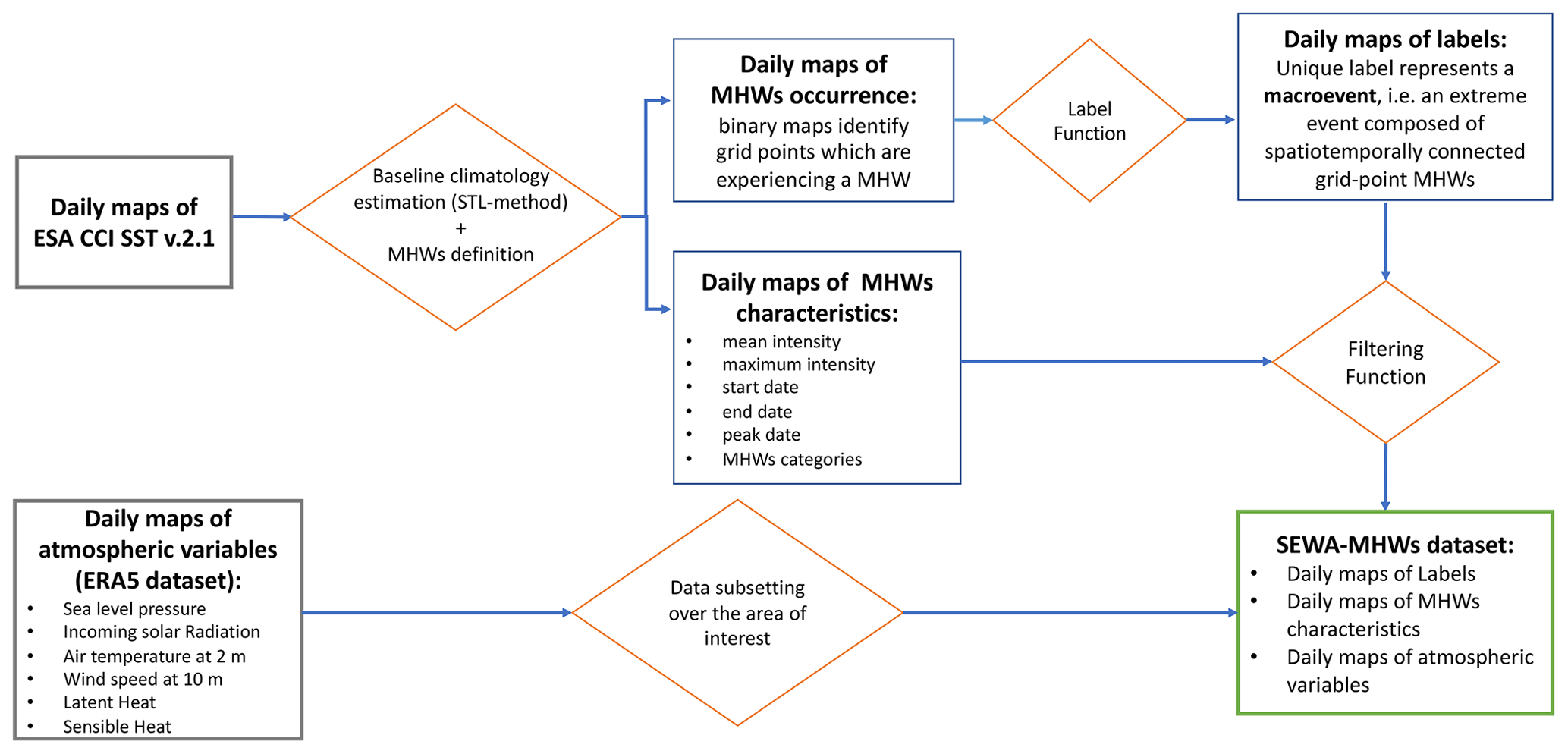
Figure 2 Flow diagram of the data processing to generate the SEWA-MHW dataset. Gray squares indicate data input. Blue squares indicate intermediate or output data. The green square indicates the final output (SEWA-MHW dataset). Orange rhombuses indicate the function/process applied.

3.1 Grid point MHW definition and their characteristics

We identified MHWs for each grid point of ESA CCI SST dataset following the definition of Hobday et al. (2016): “MHWs are identifiable events with start and end dates, a persistent duration of at least 5 d and anomalous warmer sea surface water relative to a threshold (90th or 99th percentile) in a 30-year baseline climatology”. To build a globally consistent detection framework to study MHW drivers and variability, the choice of a proper baseline climatology, along with the choice of the percentile threshold, is therefore crucial. To describe and to study MHWs, it is also fundamental to define MHW metrics and characteristics. In short, from the analysis presented in the next paragraphs, we detected MHWs for each 5 km grid for the ESA SST CCI dataset, and we obtained daily maps of MHW occurrence, i.e., binary maps identifying which of the 5 km grid points across the ocean experienced a MHW (taking the value 1 for grid points experiencing a MHW and 0 otherwise) and daily maps of MHW characteristics (Fig. 2).

3.1.1 Baseline climatology estimation and threshold

Hobday et al. (2016) estimate the baseline climatology as a seasonally varying climatology calculated over 30-year period without removing long-term trend (hereinafter the Hobday method; see Hobday et al., 2016, for details). In contrast, we considered the trend and time-varying seasonality in the baseline climatology estimation. As the definition states, MHW detection depends on the underlying SST properties (Oliver et al., 2021). Recent studies show that increases in both the mean SST and the variability in SST due to global warming can lead to the increase in warm temperature extremes (Pierce et al., 2012), so that, by the late 21st century, most of the global ocean will reach a permanent MHW state (Oliver et al., 2018; Holbrook et al., 2020; Frölicher et al., 2018). The persistent warming of SST and the increased frequency and intensity of extreme events indicate that the global ocean is experiencing unprecedented climate normals (Tanaka and Van Houtan, 2022). Thus, the rationale for considering the trend and time-varying seasonality in the baseline climatology estimation is taking into account that the mean state of the ocean is changing over time due to natural variability and anthropogenic climate change.

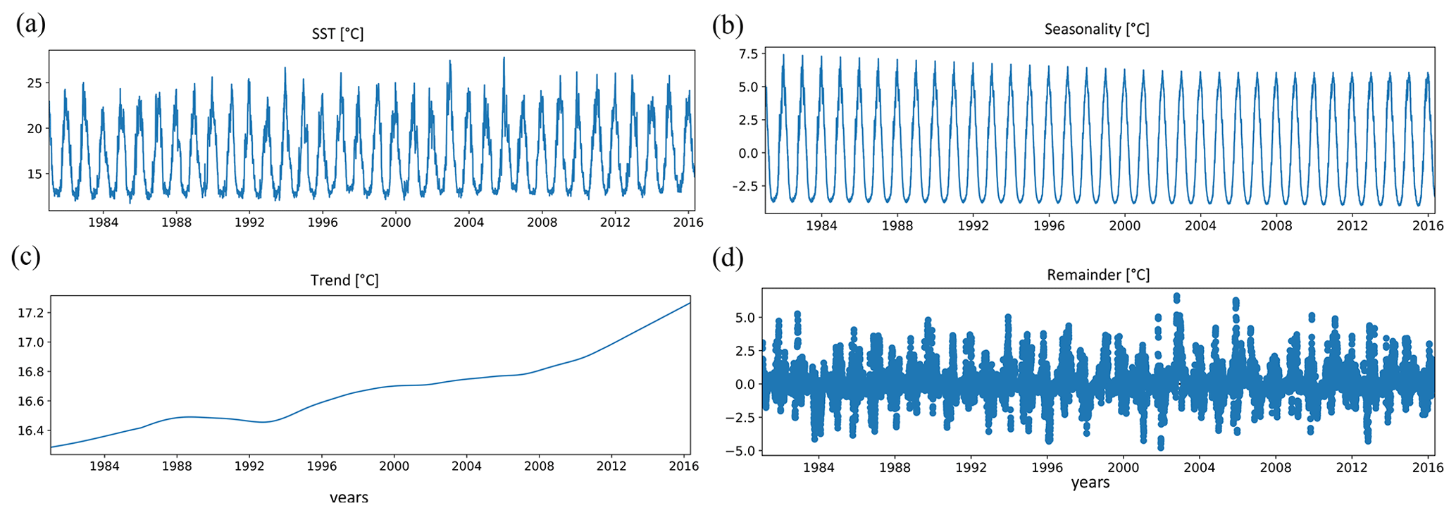
Figure 3 STL decomposition for a SST time series in the western Mediterranean (blue circle in Fig. 1a). (a) SST time series. (b) Time-varying seasonality. (c) Trend. (d) Residuals.

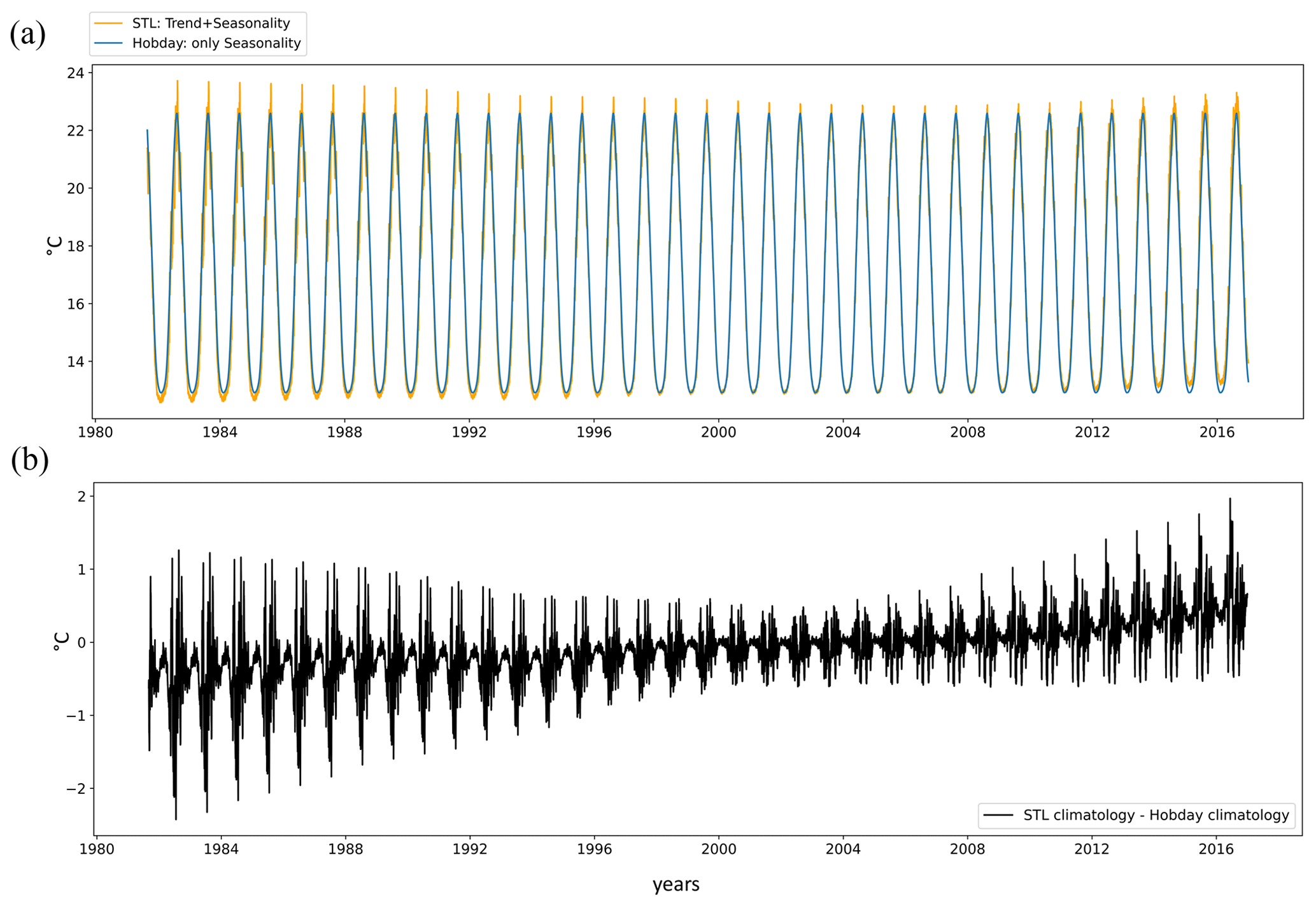
We estimated the baseline climatology using a non-parametric time series decomposition algorithm, named the Seasonal–Trend Decomposition Procedure based on LOESS (hereinafter the STL method), designed and described by Cleveland et al. (1990). It is based on the non-parametric technique known as a locally estimated scatterplot smoothing (LOESS), also commonly called a local regression. The method estimates the time-varying trend and seasonality for each time series. The STL algorithm that we applied to the ESA SST CCI is implemented in a freely available Python function named STL (https://www.statsmodels.org/devel/examples/notebooks/generated/stl_decomposition.html, last access: 14 March 2023) and accessible from the statsmodels Python package (https://www.statsmodels.org/stable/index.html, last access: 14 March 2023). Figure 3 shows the STL method decomposition for an ESA SST CCI time series in the western Mediterranean (blue circle in Fig. 1a). The main parameters to set for the STL algorithm are related to the periodicity of the seasonal signal to be extracted and to some LOESS smoothing parameters for the trend and for the seasonality. We tuned our estimation of the trend with a smoothing window of 10 years. This choice produces a trend which captures both the long-term trend and low-frequency variability (Fig. 3c). Regarding the seasonal cycle, we tuned its estimation with a yearly periodicity that was smoothed over 5 years (Fig. 3b). The time-varying amplitude of the seasonality captures increasing/decreasing trends in the seasonal variability in the time series. The sum of the trend and the seasonality is considered to be our baseline climatology (Fig. 4a; orange line).

The STL method climatology (orange line; Fig. 4a), in contrast to the Hobday method climatology (black line; Fig. 4a), varies with location, due to the trend, and in variability, due to the time-varying seasonality. The Hobday method climatology results instead in a pure periodic seasonal climatology with a flat trend. In particular, the time series of the differences between the two climatologies in Fig. 4b show an increased seasonality of the STL method climatology. The STL climatology is higher (lower) with respect to Hobday climatology during the summer (winter) season. The differences between climatologies are maximal during the 1983–1992 period for the winter season, while during the 2012–2016 period, the summer discrepancies reach 2 ^∘C due to the fact that the STL method includes an increased trend in the estimation of climatology. It is evident that SST time series could present a different time evolution. They could show decreasing, oscillating, or stationary trends in the mean and in the variance. One of the main advantages of the STL method decomposition is that it allows us to work on a SST time series in a consistent framework, where the residuals, obtained by subtracting the estimated trend and climatology from the corresponding observed SST values, are the relevant comparable series and the trend and seasonality together form the time-varying baseline climatology.

As suggested by Hobday et al. (2016), we computed the 90th percentile of the residuals and used it as threshold in order to detect the grid point MHW and obtain daily maps of MHW occurrence (Fig. 2). In addition, two successive MHW events with a 2 d or fewer time break were considered to be a single continuous event.

It is worth noting that we did not consider grid cells in which sea ice can be present, so MHWs are not available over the northern Caspian Sea or the Sea of Azov (Fig. 1).

Figure 4 (a) STL mean climatology (orange line) and Hobday mean climatology (blue line) for a SST time series in the western Mediterranean (blue circle in Fig. 1). (b) Differences between the STL mean climatology (orange line) and Hobday mean climatology (blue line) in panel (a).

3.1.2 MHW characteristics

Following the approach of Hobday et al. (2016), for each detected MHW, we calculated the following MHW metrics and characteristics, generating daily maps of MHW characteristics (Fig. 2) with the mean intensity and maximum intensity (i.e., the average and maximum temperature anomaly over the duration of the event) and the start date, the end date, and the peak date (i.e., indices at the start, end, and peak of the marine heatwave in the time series of origin). In addition, each detected MHWs was assigned to a category describing its severity (Hobday et al., 2018). These categories range from 1 to 4, and they are based on the maximum intensity in multiples of the 90th percentile exceedances, i.e., category 1 indicates that the MHW peak intensity is ≥1 times the value of the 90th percentile threshold (but less than 2 times the value). Category types are defined as 1 for moderate, 2 for strong, 3 for severe, and 4 for extreme. Note that we stored the MHW characteristics according to the day instead of according to the event, as it is usually done, so that these can be used in association with the daily maps of macroevents (see the following section).

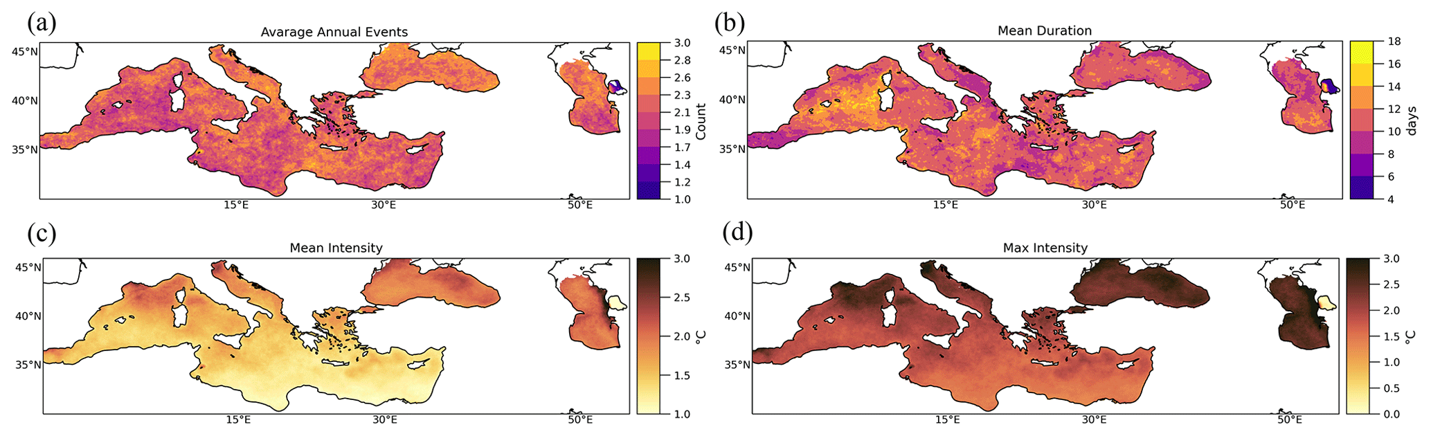
Figure 5 MHW characteristics for each grid cell. (a) Average number of annual events. (b) Mean duration. (c) Mean intensity. (d) Maximum intensity. The color schemes used in this figure are produced using the “Scientific colour maps” package (Crameri et al., 2020).

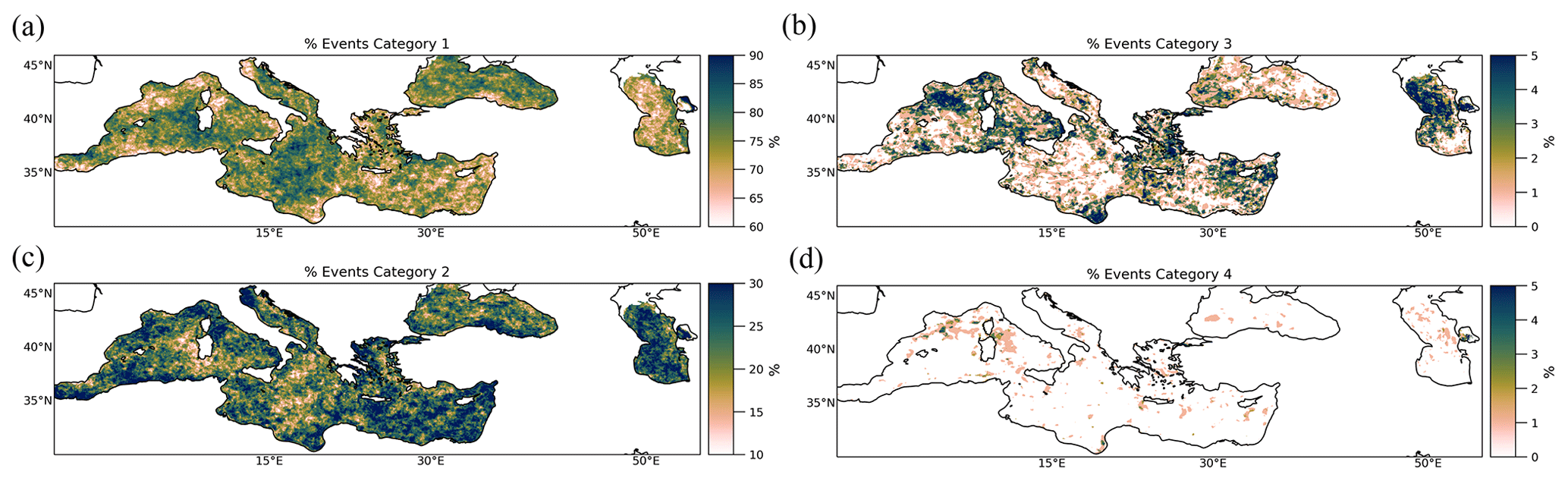
Figure 6 Percentage (%) of counted MHW events in (a) category 1, (b) category 2, (c) category 3, and (d) category 4. The color schemes used in this figure are produced using the “Scientific colour maps” package (Crameri et al., 2020).

Figure 5 shows the spatial pattern of an annual event count, the mean duration, the mean intensity, and the maximum intensity of the grid cell MHW events over SEWA basins. The Black Sea, the north Caspian Sea, the Adriatic Sea, the Gulf of Lion, and the Alboran Sea experienced the most frequent, shortest, and most intense MHWs. The majority of the events over SEWA basins belong to the moderate category, reaching 90 % in the Black Sea and in the central Mediterranean Sea (Fig. 6). All the basins experienced moderate MHWs, especially the eastern Mediterranean, the northern Adriatic, and the Ligurian seas. In total, 5 % of MHWs are severe over the eastern part of the Caspian Sea, south of the Gulf of Lion, and the Gulf of Sidra. MHWs in category 4 (extreme) are very rare in the study area.

3.2 MHW macroevents detection

The 3D binary maps (i.e., time × longitude × latitude) previously obtained were used to identify spatiotemporally connected marine heatwaves, i.e., grid points that are connected in 3D space in terms of MHW occurrence (Fig. 2). Specifically, following the approach of Woolway et al. (2021), a connected component analysis is used to identify a connected group of marine heatwave grid cells which, in turn, are considered to be part of the same MHW (i.e., a contiguous region simultaneously experiencing a MHW). For this work, we used the distributed version of the label function (https://docs.scipy.org/doc/scipy/reference/generated/scipy.ndimage.label.html#scipy.ndimage.label, last access: 14 March 2023) from the Python packaged named dask_image.ndmeasure (http://image.dask.org/en/latest/_modules/dask_image/ndmeasure.html#label, last access: 14 March 2023). The label function calculates the connectivity of features to their neighbors, based on a structuring element matrix establishing the directions in which the connectivity is defined. In our case, the inputs of the function are the 3D binary maps grouped by time (the non-zero values in matrices, i.e., MHW occurrence, in the matrices are counted by the algorithm as features; zero values are considered the background), and the structuring element matrix is orthogonal, which means that the features (i.e., grid cell MHWs) are connected in north–south and west–east directions (see the help function at http://image.dask.org/en/latest/_modules/dask_image/ndmeasure.html#label, last access: 14 March 2023, for details). Since the algorithm works in parallel, first, each chunk is independently labeled (i.e., connection in space). Then, the independent labels are made consecutive and merged along the chunks' faces whenever they are connected (i.e., connection in time). The algorithm returns the connected grid cells with a unique label. Each of these unique labels represents a macroevent. After filtering out macroevents with a maximum area lower than 100 km² (four grid cells), we found 68 068 macroevents over the SEWA region. Similarly, we also applied the filtering to the daily maps of MHW characteristics.

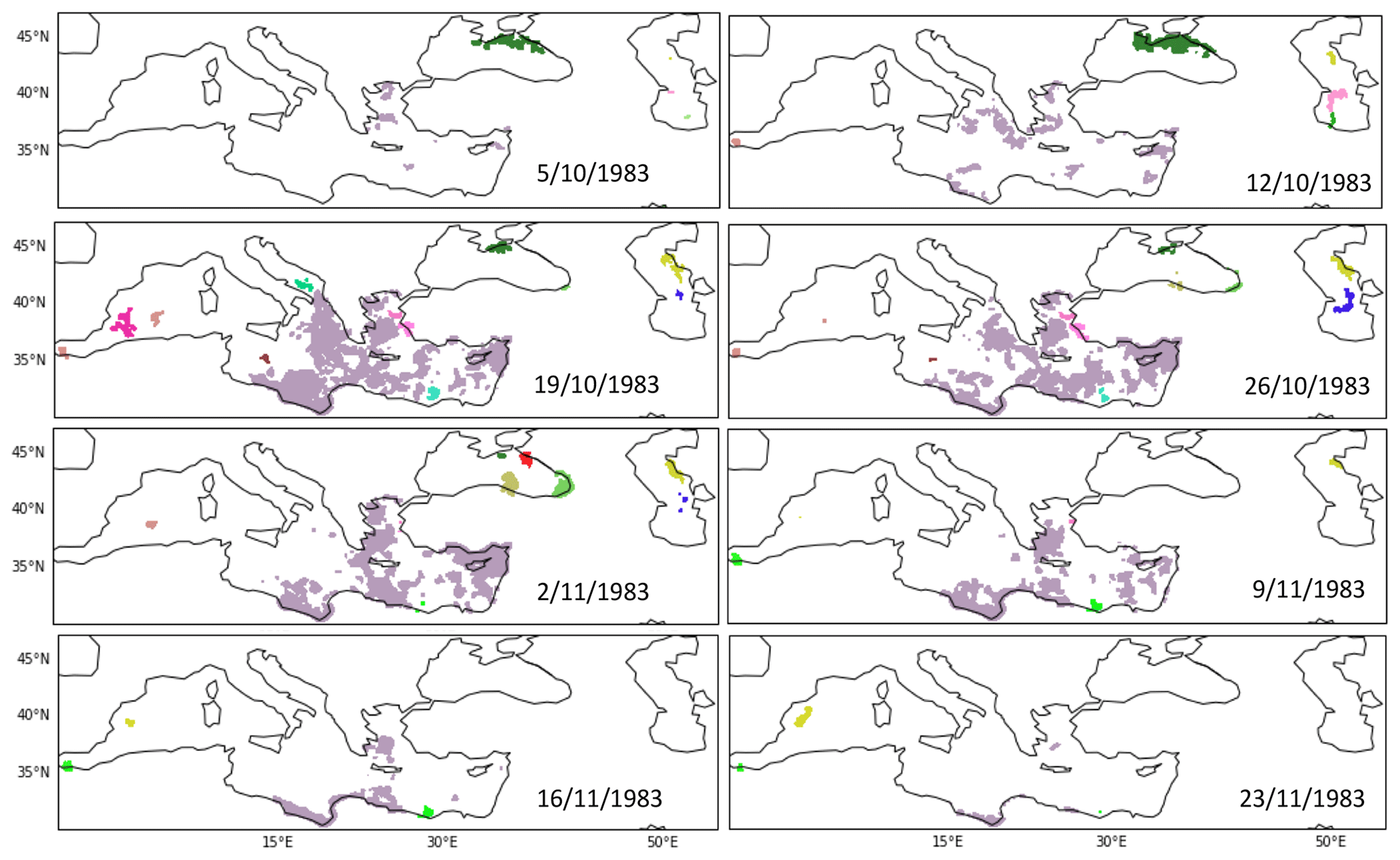
Figure 7 MHW macroevents and their evolution in time, from 5 October 1983 to 23 November 1983, over the Mediterranean Sea, as detected by the connected component analysis.

Figure 7 shows some examples of macroevents detected by our procedure and their evolution in time. Each color identifies a different macroevent. Focusing on the lilac event in Fig. 7, we can appreciate the strength of the method. The macroevent starts on 5 October in three different spots in the Aegean Sea, and then it grows spatially, reaching its maximum extension on 19 October, extending over much of the eastern Mediterranean Sea. Finally, it decays along the Libyan coast by 20 November. Meanwhile, other macroevents develop in the basins (e.g., blue label in the Caspian Sea; green label in the Black Sea). It is worth clarifying that our MHW macroevent definition does not consider the physics behind an event. As stated before, the connected component analysis is a statistical method to aggregate grid cells which are experiencing MHWs connected in time and in space. Therefore, macroevents that have been labeled differently, due to not being spatiotemporally connected (e.g., green macroevent and lilac macroevent during 9 November 1983 in Fig. 7), could have been triggered by the same causes.

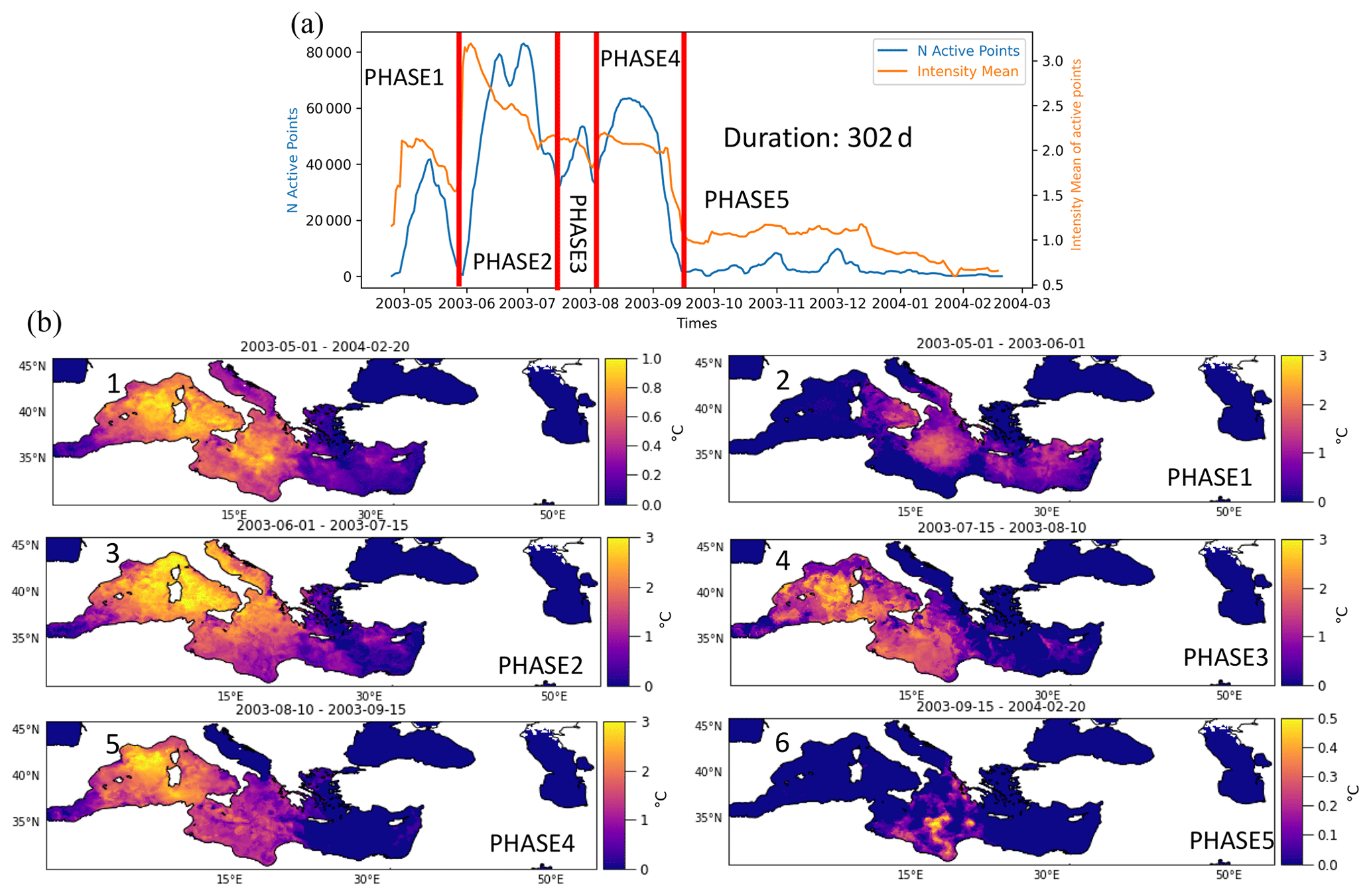
Figure 8 (a) Active points, i.e., points which simultaneously experienced the labeled MED-MHW-2003 (blue line) and mean intensity of the active points (orange) during the 2003 MHW. (b) Average of the mean intensities during the MED-MHW-2003 period (1) and during its phases (2, 3, 4, 5, and 6) computed as the sum of the MHW daily intensities divided by the duration of the phase.

Mediterranean MHW of 2003

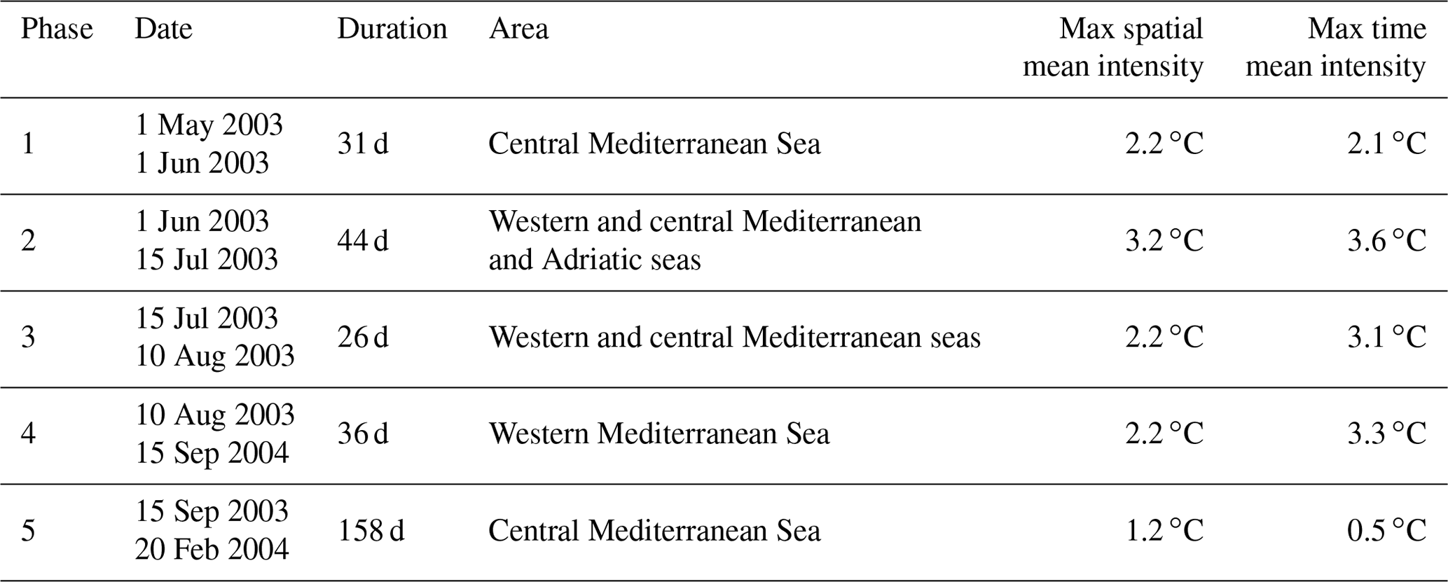
In order to assess how the proposed method performs in a case of a well-known event, we show in detail how it detected the 2003 MHW over the Mediterranean Sea (hereinafter MED-MHW-2003). The detected macroevent covered all of the western Mediterranean, and it lasted 302 d (Fig. 8a and b). Based on the number of active points (i.e., points which simultaneously experienced the labeled MED-MHW-2003; blue line in Fig. 8a) and the mean intensity of the active points (orange line in Fig. 8a), we can distinguish and characterize the evolution of the MED-MHW-2003 into five phases. The spatial patterns of the average mean intensities in Fig. 8b are computed, for each grid point, as the sum of the MHW daily intensities divided by the duration of the phase. The time series of Fig. 8a gives us information about the daily spatial mean of the MED-MHW-2003 intensities, while the spatial patterns shown in Fig. 8b teach us about the time mean of intensities during MED-MHW-2003 phases. Table 1 summarizes the characteristics of the MED-MHW-2003 phases. The phases are as follows:

1. Phase 1 lasted from May to June 2003, hitting a maximum daily spatial mean intensity of 2.2 ^∘C. It expanded over the central Mediterranean Sea. The MHW mean intensity over the entire period is around 2 ^∘C west of Sicily (Fig. 8b).

2. Phase 2 lasted from June to mid-July 2003, hitting a maximum daily spatial mean intensity of 3.2 ^∘C (Fig. 8a). It expanded over the western and central Mediterranean and the Adriatic seas. The MHW mean intensity over the entire period is around 3–4 ^∘C in the Ligurian Sea, in the Tyrrhenian Sea, and on the Adriatic coast (Fig. 8b).

3. Phase 3 lasted from mid-July to August 2003, hitting a maximum daily spatial mean intensity of 2.2 ^∘C (Fig. 8a). It expanded over the central Mediterranean Sea. The MHW mean intensity over the entire period is around 3 ^∘C to the west of Sardinia (Fig. 8b).

4. Phase 4 lasted from August to mid-September 2003, hitting a maximum daily spatial mean intensity of 2.2 ^∘C (Fig. 8a). It expanded over the western Mediterranean Sea. The MHW mean intensity over the entire period is around 3–4 ^∘C in the Gulf of Lion (Fig. 8b).

5. Phase 5 lasted from mid-September 2003 to February 2004, hitting a maximum daily spatial mean intensity of 1.2 ^∘C (Fig. 8a). It expanded over the central Mediterranean Sea. The MHW mean intensity over the entire period is around 0.5 ^∘C north of the Gulf of Sidra (Fig. 8b).

Even though the evaluation of a MHW is strictly dependent on its definition, we compared our results for the MED-MHW-2003 with existing works in the literature. Analyzing SST data from 1985 to 2003, as derived from NOAA-AVHRR measurements, Marullo and Guarracino (2003) reported a SST warm anomaly of about 4 ^∘C in June 2003 in the Gulf of Lion and the Ligurian, Tyrrhenian, northern Ionian, and Adriatic seas, which is similar to MED-MHW-2003 phase 2 (Fig. 8b). Similar to MED-MHW-2003 phases 3 and 4 (shown in Fig. 8b), they also observed the persistence of the event in July, with weaker anomalies of about 3 ^∘C, and an intensification in August over the Gulf of Lion and the Ligurian Sea, with recorded anomalies of about 4 ^∘C. In September, as detected in MED-MHW-2003 phase 5, they also observed a considerable weakening of the event, characterized by anomalies below 1 ^∘C. MED-MHW-2003 phases 1, 2, and 3 are also comparable with the analysis of Grazzini and Viterbo (2003) and Olita et al. (2007). Using the ECMWF forecast products and a regional 3-D ocean model, respectively, they described the event as being a rapid increase in the SST anomalies over the central Mediterranean Basin during May 2003, which intensified (with anomalies of about 3–4 ^∘C) and expanded, covering the whole Mediterranean, with the exception of the Aegean Sea, by the end of July. The data analyzed by Sparnocchia et al. (2006) in the Ligurian Sea evidenced the development of a warm anomaly in the SST, as reported by MED-MHW-2003 phases 2, 3, and 4. They detected a local SST anomaly up to 2–3 ^∘C, which built up at the end of May and persisted until August 2003.

Table 1 Summary of the MED-MHW-2003 phases.

3.3 SEWA-MHW dataset summary

Our dataset is composed of daily fields of macroevents and their characteristics (Fig. 2). We moved from a grid-cell-based dataset to an event-based dataset without losing grid cell information. Moreover, since the drivers and the impacts of MHWs are still not well understood, we also included, as components of the SEWA-MHW dataset, some relevant atmospheric parameters taken from ERA5 dataset (Hersbach et al., 2020) to further encourage the use of the SEWA-MHW dataset. In particular, to promote the study of the drivers, and following the work of Sen Gupta et al. (2020), we added the mean sea level pressure, the latent heat, the sensible heat, the incoming solar radiation, and the wind speed at 10 m. In addition, air temperature at 2 m is also available to promote studies on the relationship between MHWs and land heatwaves. The area extracted for these meteorological parameters is slightly bigger than the SEWA region, allowing the investigation of remote influences and/or responses of these variables in relationship with MHW macroevents. All the details, units, and names of the variables available in the SEWA-MHW dataset are explained in the Zenodo repository (Bonino et al., 2022).

4 Scientific application

4.1 Spatial/agglomerative clustering of MHW macroevents

In order to highlight the added value of the SEWA-MHW dataset, we studied the largest macroevents out of the 68 068 macroevents identified by our methodology. In particular, we classified and aggregated the largest MHW macroevents that share characteristics, taking advantage of statistical clustering methods. Following the work by Stefanon et al. (2012), who identified and classified continental heatwaves over Europe during the 1950–2009 period, we devised a clustering procedure to explore the similarities and differences among macroevents included in the dataset. Our clustering technique consists of the following four steps:

1. For each identified MHW macroevent, we extracted the maximum area extension reached. We retained MHW macroevents with an area greater than 100 000 km², which is about 25 % of the SEWA basins. We identified the 187 largest macroevents out of 68 068 macroevents.

2. For each day belonging to one event, we extracted the MHW mean intensity for all the grid points which belong to the macroevent, and we set the other grid points to none, so that, for each macroevent, we obtained daily maps of mean intensity.

3. All daily maps belonging to one macroevent are averaged, producing event maps, so that we obtained one event map of mean intensity for each macroevent.

4. An agglomerative hierarchical clustering algorithm (Gordon, 1999) is applied to the event maps. At the initial step, each event map forms a cluster. The two nearest clusters are then merged by pairing them into a new cluster. We used the cosine distances to measure the distances between the clusters. The cosine similarity is defined as the cosine of the angle between vectors (i.e., vectors of event maps); that is, the dot product of the vectors divided by the product of their lengths. The cosine similarity depends on the angle between vectors and not on their magnitudes. Therefore, the definition of the cosine distance is particularly suited to enable us to distinguish between different spatial patterns of the intensities, as it tends to increase as the number of grid cells shared by the event maps of two macroevents decreases (see Stefanon et al., 2012, for additional details). We used a Python algorithm to perform the clustering (https://scikit-learn.org/stable/modules/generated/sklearn.cluster.AgglomerativeClustering.html, last access: 14 March 2023).

Different clustering solutions have been considered, ranging from 2 to 14 clusters. Figure 9 shows the average silhouette scores obtained for each of these clustering solutions. The silhouette score is a summary of the distance between a member in a given cluster and the members in the neighboring clusters. It ranges from −1 to 1 and provides a way to assess cluster separation (Kaufman and Rousseeuw, 2009). In particular, a large average silhouette score can be considered to be an indication of large separating distances among the resulting clusters, thus implying better clustering results. According to Fig. 9a, we concluded that the optimal number of clusters is 6. In addition, the individual silhouette scores can also be exploited to investigate the quality of this optimal solution (Fig. 9b). Different colors correspond to the different clusters, and the thickness of each colored shape identifies the cluster size (i.e., number of samples, in our case event maps, in each cluster). The dashed red line shows the average silhouette score for this solution (in Fig. 9a). Most samples (i.e., event maps) have a silhouette score larger than the average score, especially in clusters 4 and 5. This indicates a favorable clustering result, in the sense that most of the samples seem to be well separated from the neighboring clusters. Nevertheless, the presence of some values smaller than the average score and negative values suggests that there is some degree of overlap among some of the clusters, with possibly misclassified events.

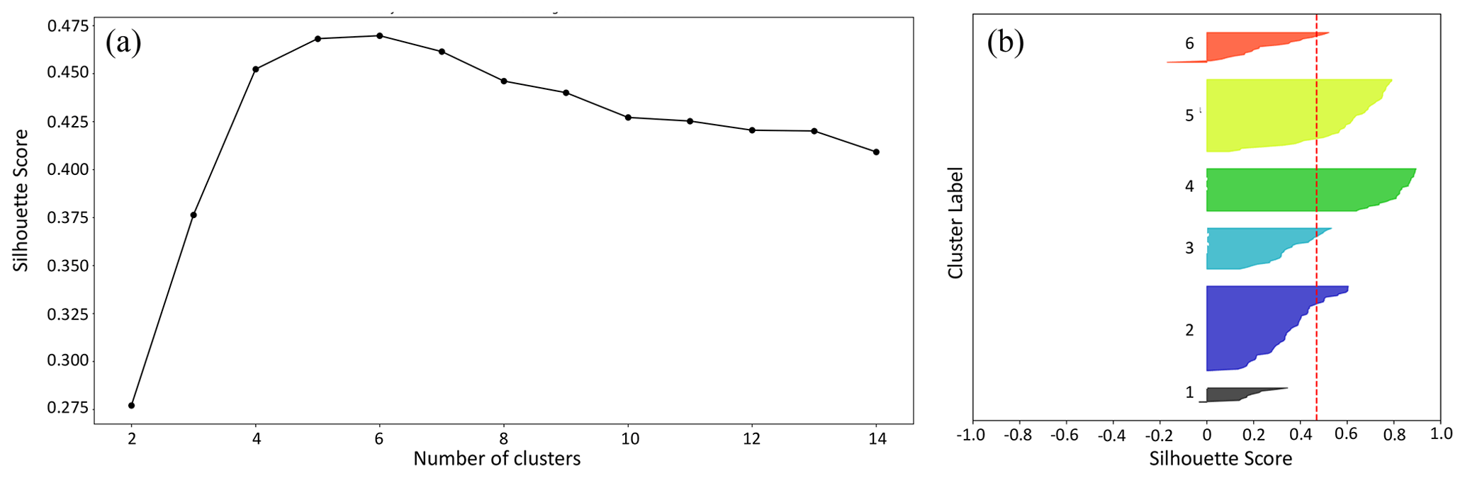
Figure 9 (a) Average silhouette score for agglomerative clustering performed using cosine distances. (b) Silhouette analysis for agglomerative clustering performed using cosine distances on data with n clusters = 6.

4.2 MHW macroevents clusters and their characteristics

Figure 10 shows the typical marine heatwave patterns for each identified cluster. The patterns of each cluster are represented by the average of the mean intensity of all the event maps which belong to that cluster. Box plots for the area maxima, duration, intensity maxima, and intensity means for MHW macroevent for each cluster are shown in Fig. 11, where the box shows the quartiles of the dataset distribution, while the whiskers extend to show the rest of the distribution, except for the diamonds that are determined to be outliers. Moreover, Fig. 12 shows the number of MHW macroevents by season and by decade for each cluster.

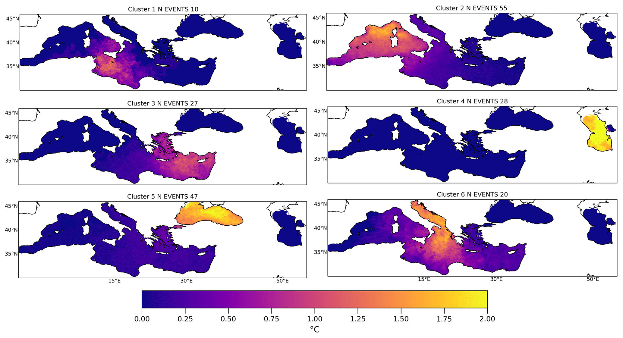
Figure 10 Patterns of the clusters represented by the average of the mean intensity of all the event maps of each cluster.

Figure 11 Box plots for (a) duration, (b) area, (c) intensity mean, and (d) intensity maxima for each cluster.

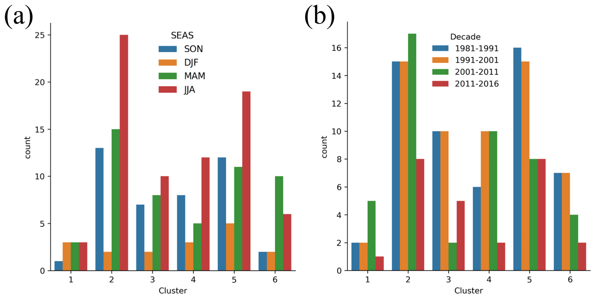
Figure 12 (a) MHW macroevents by season for each cluster. (b) MHW macroevents by decade for each cluster.

The longest and the largest macroevents, in terms of area maxima, belong to cluster 2, which spans over the western Mediterranean and the Adriatic seas. The maximum intensities are located in the Gulf of Lion and the Ligurian Sea, and they decrease in magnitude towards the Adriatic Sea. The Aegean Sea, instead, emerges as separate cluster, and it counts 27 macroevents (cluster 3 in Fig. 10). The maximum intensities are located west of Cyprus, and they decrease in magnitude around the Aegean Islands, showing a mean intensity of about 1.3 ^∘C and a maximum intensity of about 2.5 ^∘C (Fig. 11). The Aegean Sea, to a lower extent, is also part of other two identified clusters, namely cluster 5 and cluster 6. The former expands into the Black Sea, where it shows its maximum intensity, while the latter includes the Adriatic Sea and the Ionian Sea. Both of these two clusters experienced strong macroevents with a maximum intensity of about 3.5 ^∘C (Fig. 11). Apart from cluster 6, the central Mediterranean Sea is also home of the smallest cluster, consisting of 10 macroevents confined from the Strait of Sicily to the eastern Libyan coast (cluster 1 in Fig. 10). The maximum intensities are located south of Sicily, with a mean intensity of about 1.3 ^∘C and a maximum intensity of about 2.5 ^∘C (Fig. 11). A completely isolated cluster groups the 28 macroevents over the Caspian Sea (cluster 4 in Fig. 10). The maximum intensities are located along the western coast of the basin. The strongest, in term of intensity, macroevents belong to this cluster, reaching 2.3 and 4.5 ^∘C for mean and maximum intensity, respectively (Fig. 11).

Except for cluster 6 and cluster 1, it is interesting to highlight that the majority of the events are during the summer, while the winter produced only a few macroevents for each cluster (Fig. 12). Moreover, we do not report an increasing number of MHWs during the last 6 years (2011–2016), as reported by Dayan et al. (2022). Actually, the majority of the macroevents in almost all of the clusters occurred during the first 2 decades of the studied period (Fig. 12). This is likely linked to the fact that we considered the trend in the baseline climatology estimation (see Sect. 3.1.1).

Our clustering methodology seems to be effective in distinguishing different spatial patterns of MHW macroevents over the SEWA basins. The macroevent results are geographically confined to the closed basins (i.e., Caspian Sea and Black Sea) or to the sub-basins of the Mediterranean Sea (e.g., western Mediterranean Sea); however, this highlights some relations between adjacent sea regions (e.g., Adriatic Sea and Aegean Sea; cluster 6).

5 Code and data availability

The SEWA-MHW dataset that consists of daily fields of MHW macroevents, their characteristics, and relevant atmospheric variables is stored in the Zenodo archive (Bonino et al., 2022, https://doi.org/10.5281/zenodo.7153255). The MHW detection methodology described in Sect. 3 is applied to the SEWA region, but it could be, in principle, applied to the global ocean or to other basins. Moreover, the SEWA-MHW dataset is inevitably linked to the ESA CCI SST dataset; indeed, all the datasets that are produced from or reuse high-quality data depend on the data used to generate them. Even though the routines are computational and time-demanding, we provide scripts to rerun the method over other regions or use other and updated SST datasets. We provide the code to detect MHWs and their characteristics (MHWs_stl.ipynb), the code to generate the MHW macroevents (SEWA_LABEL.ipynb), and the code to filter out the smallest macroevents (MHWs_filter.ipynb). The codes are also available in the Zenodo repository. Please refer to the dataset description in Bonino et al. (2022) for any details on the NetCDF files and on the codes.

6 Summary and outlook

In this work, we presented a dataset of marine heatwave macroevents and their characteristics over the southern Europe and western Asian basins during the 1981–2016 period that is named SEWA-MHW. We obtained the dataset by analyzing the observed SST provided by the European Space Agency, the ESA CCI SST v2.1 dataset (Merchant et al., 2019). Briefly, we defined MHWs in each 5×5 km grid point of the ESA CCI SST dataset, and then, using a connected component analysis, we aggregated the spatiotemporally connected MHWs (i.e., grid points that are connected in 3D space in terms of marine heatwave occurrence) in order to obtain MHW macroevents. As a result, the SEWA-MHW dataset consists of a daily field of MHW macroevents and their characteristics.

The methodological framework used to build SEWA-MHW dataset is the novelty of this study with respect to the existing literature (e.g., Darmaraki et al., 2019; Sen Gupta et al., 2020; Oliver et al., 2021). First, the detected MHWs in the ESA CCI SST dataset are relative to a time-varying baseline climatology, which considers both the trend and seasonal variability to mimic the changing of the climate mean state. Second, the connected component analysis allow us to aggregate the MHWs connected in time and in space and to pass from a the grid-cell-based dataset to an event-based dataset without losing high-resolution (i.e., grid cell) information. This approach, different from the previous studies, provides the time evolution of the event at the basin scale. Even though the evaluation of a MHW is strictly dependent on its definition, we demonstrated that our method is effective in detecting MHW macroevents. The well-known MHW of 2003 in the Mediterranean Sea is comparable with the records (e.g., Olita et al., 2007; Sparnocchia et al., 2006; Marullo and Guarracino, 2003; Grazzini and Viterbo, 2003).

To the best of our knowledge, the SEWA-MHW dataset is the first effort in the literature to archive extremely hot sea surface temperature macroevents. The advantages of the availability of a MHW macroevent dataset are avoiding wasting computational and/or time resources to process SST data to detect MHWs and building a consistent framework which would increase comparability among MHW studies. As Pastor and Khodayar (2022) and Sun et al. (2022) suggested in very recent papers, the scientific community should focus on establishing a universal definition of MHW events which does not rely only on the grid cell definition. Besides the consistency ensured among MHW studies that will use the SEWA-MHW dataset, the SEWA-MHW dataset also provides a ready-to-use dataset to be compared to other studies which apply different MHW definitions. On top of that, Pastor and Khodayar (2022) also suggest that it should be mandatory to introduce some spatial limitations in the study of MHWs, especially when targeting impacts. Our users could, as we did for the statistical clustering, filter out macroevents based on their needs. The SEWA-MHW dataset can be used for many scientific applications. For instance, we efficiently clustered the biggest SEWA-MHW macroevents that share common features and characteristics in order to report on and to characterize typical spatial patterns of MHWs over SEWA basins. Indeed, the employed clustering method was able to distinguish different spatial patterns of MHW macroevent.

The SEWA-MHW dataset is also suitable for regional and coastal MHW studies, due to its high resolution, and it is expandable to all the ocean basins to provide global coverage. Moreover, the synergistic use of the SEWA-MHW dataset with other model outputs and observation data could help to fill the knowledge gaps about the drivers and the marine ecosystem impacts of these extreme events. Recently, compound events have become of particular interest; i.e., when conditions are extreme for multiple potential ocean ecosystem stressors such as temperature and chlorophyll (Gruber et al., 2021; Le Grix et al., 2021). On top of that, this synergistic use of the SEWA-MHW dataset with other datasets could facilitate the building of a prediction scheme using, for example, deep machine learning approaches. These techniques need large and high-resolution datasets to be trained and tested.

In a broader perspective, the novel science resulting from the aforementioned exploitation of the SEWA-MHW dataset could be transferred to solutions and advanced decision support systems for society.