MDAS: a new multimodal benchmark dataset for remote sensing

In Earth observation, multimodal data fusion is an intuitive strategy to break the limitation of individual data. Complementary physical contents of data sources allow comprehensive and precise information retrieval. With current satellite missions, such as ESA Copernicus programme, various data will be accessible at an affordable cost. Future applications will have many options for data sources. Such a privilege can be beneficial only if algorithms are ready to work with various data sources. However, current data fusion studies mostly focus on the fusion of two data sources. There are two reasons; first, different combinations of data sources face different scientific challenges. For example, the fusion of synthetic aperture radar (SAR) data and optical images needs to handle the geometric difference, while the fusion of hyperspectral and multispectral images deals with different resolutions on spatial and spectral domains. Second, nowadays, it is still both financially and labour expensive to acquire multiple data sources for the same region at the same time. In this paper, we provide the community with a benchmark multimodal data set, MDAS, for the city of Augsburg, Germany. MDAS includes synthetic aperture radar data, multispectral image, hyperspectral image, digital surface model (DSM), and geographic information system (GIS) data. All these data are collected on the same date, 7 May 2018. MDAS is a new benchmark data set that provides researchers rich options on data selections. In this paper, we run experiments for three typical remote sensing applications, namely, resolution enhancement, spectral unmixing, and land cover classification, on MDAS data set. Our experiments demonstrate the performance of representative state-of-the-art algorithms whose outcomes can serve as baselines for further studies. The dataset is publicly available at https://doi.org/10.14459/2022mp1657312 (Hu et al., 2022a) and the code (including the pre-trained models) at https://doi.org/10.5281/zenodo.7428215 (Hu et al., 2022b).

1 Introduction

The rapid development of Earth observation (EO) techniques enables the measurements and monitoring of Earth on the land surface and beneath, of the quality of air and water, and of the health of humans, plants, and animals. Remote sensing (RS) is one of the most important contact-free sensing means for EO to extract relevant information about the physical properties of the Earth and environment system from space. With the ever-growing availability of RS data source from both satellite and airborne sensors on a large scale and even global scale, e.g. Sentinel missions, multi-modal RS techniques have been garnering increasing attention in various EO-related tasks (Hong et al., 2021c). The data acquired by different platforms can provide diverse and complementary information, such as light detection and ranging (lidar) providing the height information about the ground elevation, synthetic aperture radar (SAR) providing the structure information about Earth's surface, and multispectral (MS) or hyperspectral (HS) data providing detailed content information of sensed materials. The joint exploitation of different RS data has been therefore proven to be helpful to further enhance our understanding, possibilities, and capabilities to Earth and environment.

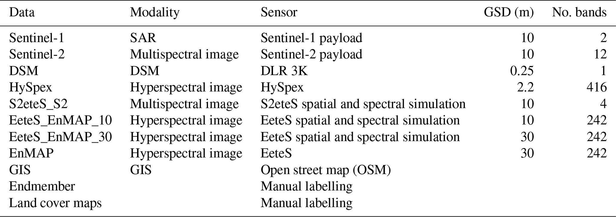
Table 1 Remote sensing data sets comparison. MDAS offers five data modalities, carefully prepared and collected on a single day, thus its content is nearly identical across modalities.

Multimodal data fusion takes advantage of complementary information of different data sources so that its performance can reach beyond the limitation of individual data. Currently, a lot of studies in remote sensing focus on developing methodologies that can effectively utilize different data sources. Tupin and Roux (2003); Hu et al. (2019); Hong et al. (2020c); Meraner et al. (2020); Adrian et al. (2021); Hong et al. (2021f) develop algorithms to join advantages of optical images and synthetic aperture radar (SAR) data for their respective goals. They utilize spatial structures, spectral information from optical data, and the independence of weather conditions, dielectric properties, and geometric structures from SAR data. Paris and Bruzzone (2014); Khodadadzadeh et al. (2015); Al-Najjar et al. (2019); Hang et al. (2020); Ge et al. (2021); Hong et al. (2020a) introduce models to merge height information from lidar data or digital surface model (DSM) with spatial and spectral information from optical images. Yokoya et al. (2011); Simoes et al. (2014); Hong et al. (2019b, c); Zhang et al. (2020c); Liu et al. (2020) propose methods to fuse rich spectral information of hyperspectral images with high spatial resolution of multispectral images. All these studies have proven that the data fusion is very beneficial to remote sensing applications.

While reviewing literature of data fusion, one can find that some data sets frequently appear in a lot of studies, for example, the hyperspectral image of Houston university (https://hyperspectral.ee.uh.edu/?page_id=1075, last access: 2 January 2023) and the aerial images and DSM of Vaihingen (Rottensteiner et al., 2012). These accessible benchmark data sets play a very important role in the advancing of fusion technologies. Especially, in this era, data are the foundation for state-of-the-art machine learning and deep learning methodologies. As remote sensing data strongly associate to geographic locations, it would be beneficial to the community to have more benchmark data sets of high quality that originate from different geolocations.

In the remote sensing community, benchmark data sets are often generated based on one data source, such as the UC-Merced dataset (Yang and Newsam, 2010), the WHU-RS19 dataset (Xia et al., 2010), the AID dataset (Xia et al., 2017), the Berlin-urban-gradient (Okujeni et al., 2016), the SAR-Ship (SSDD, Zhang et al., 2021), DOTA (Xia et al., 2018), and the BigEarthNet (Sumbul et al., 2019). Recently some researchers created benchmark data sets for multimodal remote sensing data, such as Hong et al. (2021e), including hyperspectral and multispectral data, hyperspectral and SAR data, hyperspectral, SAR, and DSM data, or DFC 2018 (Xu et al., 2019) and So2Sat LCZ42 (Zhu et al., 2020). Besides this, the IEEE GRSS data fusion contests have done great contributions by consistently publishing data sets for developing fusion technologies. They often provide two to three types of data for tasks like classification, detection, and 3D reconstruction (Wu et al., 2019, 2020). By far, the listed datasets mostly have a comparative large amount of samples and wide geographic distribution because it is easy to access the original data sources, such as Sentinel-1, Sentinel-2, and Google Earth images. When involving certain data sources, namely, hyperspectral image, lidar data, and DSM, the amount of samples is often limited due to the high costs of collections and data preparations. Examples are the Vaihingen dataset and the Houston dataset. The complexity of preparing these data is also one of the reasons that most studies focus on fusing two data sources, often the easily accessible ones. Table 1 summarizes the characteristics of some of the most popular data sets in the field.

In this paper, we contribute to the community by publishing a benchmark remote sensing dataset including five modalities, namely, SAR data, multispectral image, hyperspectral image, DSM, and GIS data, for the entire city of Augsburg, Germany. Apart from the GIS data, the remote sensing data are all collected on the same day. The preparations of the SAR data, the hyperspectral image, and the DSM are carried out by a group of experienced experts to ensure the high quality. We also provide experiment results of state-of-the-art algorithms in this paper for three typical remote sensing tasks, namely, resolution enhancement, spectral unmixing, and land cover classification. These results play as baselines for future studies. MDAS not only provides one more testing instance for developing algorithms of typical tasks, but also possibilities for unknown applications because of the variety of data modalities.

1.1 Super-resolution

Images with high spatial resolution have detailed textures and structures that facilitate semantic interpretation. Meanwhile, materials have different reflectances at different ranges of wavelengths, a high spectral resolution and a wide spectral range can benefit the identification of covering material. However, the limitation of imaging sensors prevents achieving high resolution in spectral and spatial domains at the same time (Loncan et al., 2015; Hong et al., 2021g). To break the limitation, researchers develop super-resolution algorithms to fuse data of the two types so that high resolution in both spatial and spectral domains are available. With the increasing amount of multispectral and hyperspectral data, e.g. Sentinel-2 images and EnMAP images, the super-resolution products have an important role in optical remote sensing.

Current super-resolution research (Sheikholeslami et al., 2020; Yokoya et al., 2017; D. Zhang et al., 2020; S. Zhang et al., 2020b) evaluates algorithms based on data sets which have high spatial resolutions. They down-sample the spatial resolution of original data sets to create the counterpart low resolution data. On spectral domain, they mostly apply either the same spectral bands or a subset of the spectral bands. Very few would utilize simple spectral response functions. These data configurations simplify the super-resolution applications of the real world. In this regard, in MDAS, we attempt to provide realistic data sets. We simulate EnMAP and Sentinel-2 images using the EeteS (Segl et al., 2012, 2010) and S2eteS (Segl et al., 2015) software based on a HySpex imagery. This simulation integrates not only the specific spatial response functions and spectral response functions, but also the effects of instrumental and environmental parameters on the resulting image characteristics. Besides the simulations, we also provide a Sentinel-2 image from the same date for the same region.

When comparing to the current data sets used for super-resolution evaluations that mostly only emphasize the spatial resolution, MDAS also challenges the algorithms with respect to spectral enhancement, instrumental effects, environmental impact, and influence of different sensors.

1.2 Spectral unmixing

Hyperspectral remote sensing has greatly improved our ability to qualitatively and quantitatively sense Earth’s surface, due to its capability to obtain data with tens to hundreds of contiguous spectral bands (Hong et al., 2020b). However, mixed pixels are widely spread in hyperspectral image due to its limited spatial resolution, which has hindered the accurate analysis and applications of hyperspectral data. Hyperspectral unmixing is one of the most hot topics i hyperspectral image processing, which aims at solving the mixed pixel problem by decomposing the mixed pixel into the constituent pure signatures, also called endmembers, and the corresponding abundance coefficients (Liu et al., 2017; Hong et al., 2021d).

The unmixing topic has been intensively studied by researchers in the last few decades, and many efforts have been made to improve the accuracy of the methods of unmixing. The most widely used real hyperspectral image datasets for the evaluation of the developed unmixing algorithms were presented by Zhu (2017), in which the Urban dataset and Cuprite dataset are exceedingly frequently used. These images are small in spatial size, which is not enough to test whether the developed method is capable of processing large dataset with low error and reasonable time cost. Hong and Zhu proposed a novel subspace unmixing framework with the use of low-rank attribute embedding, called SULoRA (Hong and Zhu, 2018). Moreover, they further considered the spectral variability, and proposed a seminal linear mixing model, called augmented linear mixing model (ALMM) for accurate spectral unmixing (Hong et al., 2019a). In addition, the ground truth of abundance is usually not available and only synthetic images can be used for the quantitative evaluation of the abundance (Du et al., 2019). However, synthetic images cannot model the complex scene of real images. Thus, large dataset with reliable reference is highly requested for the development of efficient unmixing methods.

1.3 Multimodal land cover classification

Land cover classification has been a fundamental but challenging research topic in the RS community, as many high-level subsequent analysis largely depends on the classification results. Over the past decades, extensive classification algorithms were developed for single modalities (Huang et al., 2020; Hong et al., 2021b; Rasti et al., 2020), e.g. HS, MS, SAR, lidar, OpenStreetMap. These methods have been proven to be effective in many real applications. We have to admit, however, that the utilization of single modalities inevitably suffers from the performance bottleneck. Enormous efforts have been recently made to couple or jointly analyse different RS observation sources by the attempts to design advanced data fusion methods to achieve a more diversified description for a studied scene. According to different processing levels that the fusion behaviour happens, the current state-of-the-art approaches related to RS data fusion can be approximately categorized into three groups: data level, feature level, and decision level.

The first application of this paper, i.e. HS super-resolution, is a typical data level fusion task. These developed super-resolution approaches are only applied for homogeneous RS data fusion, e.g. HS and MS images and panchromatic and MS images. Because they have a similar imaging principle and data structure, enabling the fusion of these data sources. For heterogeneous RS data, e.g. SAR and optical data, DSM and SAR, or DSM and optical data, they fail to directly fuse in the image level due to their totally different image properties and structure. For this reason, the feature level fusion strategy has been garnering increasing attention, providing greater potential in the land cover classification task. Very recently, only few benchmark datasets are openly available for multimodal RS data processing and analysis, e.g. land cover classification. More notably, there are some potential limitations in these existing and public benchmark datasets. For example,

• the number of multimodal RS data are limited, e.g. the well-known Houston 2013 datasets (including HS and DSM data) provided by the IEEE Data Fusion Contest (DFC) 2013, the LCZ datasets (including MS and OpenStreetMap) provided by the IEEE DFC 2017, the optical and lidar data provided by the IEEE DFC 2019;

• there is a lack of diverse multimodal data, especially heterogeneous data, e.g. the Houston 2018 datasets provided by the IEEE DFC 2018, including HS, MS, RBG.

For these reasons, building high-quality and multimodal RS benchmark datasets is a primary and key step to boost the development of various multimodal RS applications, further contributing to the RS community. This, therefore, will motivate us to develop new and more diversified multimodal RS datasets.

1.4 Contribution of this paper

In this paper, we have two major contributions. First, we publish MDAS, a new multimodal benchmark data, that consists of five modalities. All components of MDAS are well-prepared by experienced experts to ensure a high quality, e.g. the preparation of the DLR 3K DSM, the simulation of EnMAP imagery, and the generation of ground reference for unmixing. As far as we know, the ground reference is the first product that provides reliable reference for quantitative evaluation of real hyperspectral image unmixing. Besides the high quality, the variety of data modality provides more possibilities for data fusion applications. Second, we demonstrate the performance of state-of-the-art algorithms for three typical remote sensing applications, namely, resolution enhancement, spectral unmixing, and land cover classification. These experiment results provide baselines for further algorithm developments on MDAS.

2 MDAS dataset

MDAS has remote sensing data of five modalities. They are SAR data, multispectral image, hyperspectral image, DSM, and GIS data. Figure 1 demonstrates all these modalities. The region of interest (ROI) is the city of Augsburg, Germany, and covers an area of 121.7 km². Apart from the GIS data, the other data are all collected on the same day, 7 May 2018.

Figure 1 The visualization of five data modalities in MDAS. From left to right: the Sentinel-1 image (VH band in dB), the Sentinel-2 image (RGB: 665, 560, 490 nm), the OSM land use layer, the HySpex image (RGB: 691, 569, 445 nm), and the DSM.

2.1 Synthetic aperture radar data

The SAR component in MDAS is a Sentinel-1 data. The SAR data after processing is the backscattering coefficient. No speckle denoising was applied and the data were not converted to dB. We download a level-1 Ground Range Detected (GRD) product collected under the Interferometric Wide (IW) swath mode. It is a dual-Pol SAR data with VV and VH channels. Based on recommended preprocessing of Sentinel-1 data in Hu et al. (2018); Filipponi (2019); Zhu et al. (2020), we prepare the SAR data by using ESA SNAP toolbox (https://step.esa.int/main/toolboxes/snap/, last access: 2 January 2023) following the workflow of applying precise orbit profile, conducting radiometric calibration, and performing terrain correction. The topographic data used in the processing are from the Shuttle Radar Topography Mission (SRTM). We apply bilinear interpolation to achieve a geocoded SAR image with a 10 m ground sampling distance (GSD). Based on the ROI, the final SAR image has a size of 1371×888 pixels, a geographic reference of WGS 84/UTM zone 32 N, and two channels (intensities of VV and VH).

2.2 Multispectral imagery

The multispectral imagery in MDAS is a Sentinel-2 data. We fetch a level-2A product directly from the Sentinel Data Hub. It is an image in bottom of atmosphere (BOA) reflectance and geocoded in WGS 84/UTM zone 32 N as well. It has 12 spectral bands with wavelength ranging from 440 to 2200 nm. The six bands (B5, B6, B7, B8A, B11, B12) of 20 m GSD and the two bands (B1, B09) of 60 m GSD are all upsampled to 10 m GSD. The final image is cropped according to the ROI, resulting in a size of 1371×888 pixels.

2.3 Hyperspectral imagery

2.3.1 Data acquisition

The hyperspectral images used in this study have been acquired using the airborne imaging spectrometer system HySpex, which is operated by the Remote Sensing Technology Institute (IMF) of the German Aerospace Center (DLR). For this study, HySpex was mounted on a Dornier DO228-212. The imagery over the city of Augsburg was acquired in 23 flight strips.

2.3.2 System configuration

The system features two different cameras covering the VNIR (visible and near-infrared) and SWIR (shortwave infrared) spectral domain. Both cameras have been extensively characterized at the Calibration Home Base (CHB, Brachmann et al., 2016), resulting in a very well characterized high-precision instrument suited for benchmark Earth observation applications. The HySpex VNIR-1600 features a CCD detector covering the spectral range 416 to 992 nm with 160 channels. This results in a spectral sampling interval of 3.6 nm. The spectral resolution ranges from 3.5 nm at nadir to approximately 6 nm at the outer edge of the swath. The HySpex SWIR-320m-e is equipped with a mercury cadmium telluride (MCT) detector with 256 channels covering the spectral range 968 to 2498 nm at a sampling interval of 6 nm and a spectral resolution of 5.6 to 7.0 nm. The VNIR detector has a width of 1600 pixels, while the SWIR detector has a width of 320 pixels (Köhler, 2016).

2.3.3 Preprocessing

The HySpex processing chain consists of two parts: The preparation of the data for the automatic processing, which comprises the processing of GPS and IMU data and assigning them to the corresponding flight strips, and the second part consisting of systematic correction, orthorectification, co-registration, and atmospheric correction, which is performed in the generic processing system Catena (Krauß et al., 2013). For the systematic correction, the following steps are applied on each frame in the given order: dark signal correction, linearity correction (VNIR only), stray light correction (VNIR only), radiometric calibration, bad pixel correction (SWIR only), and finally correction of point spread function (PSF) non-uniformities. The linearity correction of the VNIR instrument is performed after the dark signal correction, since the dark current is very stable and does not significantly change. For the stray light correction, a four-dimensional tensor is applied. Currently, only the VNIR data are corrected for stray light, while the measurement of the SWIR instrument's stray light is currently ongoing research. The radiometric calibration is performed by dividing the signal corrected to this point by the radiometric response multiplied by the integration time. The radiometric responses of both instruments are determined during laboratory calibration. The bad pixels of the HySpex SWIR are corrected by linear interpolation between adjacent pixels along the spectral axis, while the bad pixels of the VNIR are corrected by the camera software. Finally, optical distortions like smile, keystone, and – equally important – the individual angular and spectral resolutions of each pixel are corrected by applying an individual homogenization kernel to each pixel. For the co-registration of VNIR and SWIR data, a BRISK matching is used (Schwind et al., 2014). After this step, the data are orthorectified using the physical sensor model, the GPS-/IMU-data, the mounting angles, and the DEM by the DLR software ORTHO, followed by an atmospheric correction using the DLR software ATCOR (Richter, 1998). As reflectance depends on the viewing and solar illumination geometry, the processed data strips appear inconsistently in magnitudes, which results in different brightness. This phenomenon is described by the bidirectional reflectance distribution function (BRDF). We manually iterate a BRDF effects correction routine (BREFCOR, Schläpfer et al., 2014) on our imagery and dramatically mitigate the influence of BRDF. At last, the data strips are merged as one scene for the entire city of Augsburg.

2.3.4 Simulation of additional image products

The hyperspectral Augsburg mosaic is an ideal data basis to derive further image products suitable for classification tests or resolution enhancement experiments. Accordingly, very realistic hyperspectral EnMAP and multispectral Sentinel-2 data were generated. This was done using the EeteS (Segl et al., 2012, 2010) and S2eteS (Segl et al., 2015) software, both developed within the EnMAP project (Guanter et al., 2015) to understand better the effects of instrumental and environmental parameters on the resulting image characteristics. The sequential processing chain of these software tools consists of four independent parts – the atmospheric, spatial, spectral, and radiometric modules – in which the HySpex BOA reflectance data are used to calculate top-of-atmosphere radiance and subsequently digital numbers. This forward simulator is coupled with a backward simulation branch consisting of calibration modules (e.g. for EnMAP: non-linearity, dark current, and absolute radiometric calibration) and a series of pre-processing modules (radiometric calibration, co-registration, atmospheric correction, and orthorectification) forming the complete end-to-end simulation tool. Since both image products are based on the same data, they are ideally suited for comparisons of classifications or parameter retrievals using EnMAP and Sentinel-2 images. Additional three images were generated for resolution experiments, which do not contain any additional sensor or processing uncertainties for better comparison. Accordingly, an end-to-end simulation was completely omitted here and only a purely spectral and spatial adaptation was calculated. In a first step, the HySpex data were spatially adjusted to 10 and 30 m GSD, respectively. This was done with the help of a PSF convolution using a 2D Gaussian filter, whose full width at half maximum (FWHM) results from the ratio of the output and input GSD. Since the input grid (2.2 m grid size) and output grids ($\mathrm{10.0}/\mathrm{30.0}$ m) do not overlap perfectly, the result of the PSF convolution is slightly erroneous because the PSF cannot be perfectly positioned over the input pixels. In order to keep these errors as small as possible, the PSF was spatially shifted in the Fourier space for each pixel and thus optimally adapted to the input grid. Subsequently, the 10 and 30 m GSD data were spectrally adjusted to the 242 EnMAP bands by a spectral filtering using the original spectral response functions of ENMAP. Similar, the four Sentinel-2 10 m bands were also generated based on the 10 m GSD data.

Figure 2 Shaded DSM of subarea.

2.4 Digital surface model

A high-resolution DSM with images acquired with the 3K camera system (Kurz et al., 2012) has been generated for this study (see example of sub area in Fig. 2). For this, 1702 images from the nadir-looking camera, which has an average coverage of 1170 m × 765 m and a GSD of 25 cm, were used for the further processing. These images were acquired with 23 flight strips covering the whole test area of 275 km² size at a flight height of 1800 m above ground, which results in a 75 % and 36 % along, respectively, across-track overlap. First, a self-calibration image bundle adjustment was performed using the SAPOS corrected and filtered GNSS/inertial data of the image positions and attitudes as well as 121 116 tie points. No further pass information was introduced, except the global SRTM elevation model as a weak additional height information for the tie points. With precise oriented images, the DSM generation was then performed using the SGM algorithm with modifications (d'Angelo and Kurz, 2019). The resulting disparity images for each stereo pair were filtered, fused, filled, and finally resampled to a GSD of 30 cm.

2.5 Geographic information system (GIS) data

For the GIS data in MDAS, we download the building layer, the land use layer, and the water layer from Open Street Map (https://www.openstreetmap.org/#map=13/48.3699/10.8809, last access: 2 January 2023). The original vector layers are rasterized into GeoTiff files with a coordinate system of WGS 84/UTM zone 32 N. Depending on the application, the GIS data can be utilized as either input data or ground reference.

Figure 3 Three manually labelled subregions.

Figure 4 The endmember spectra for each land cover class.

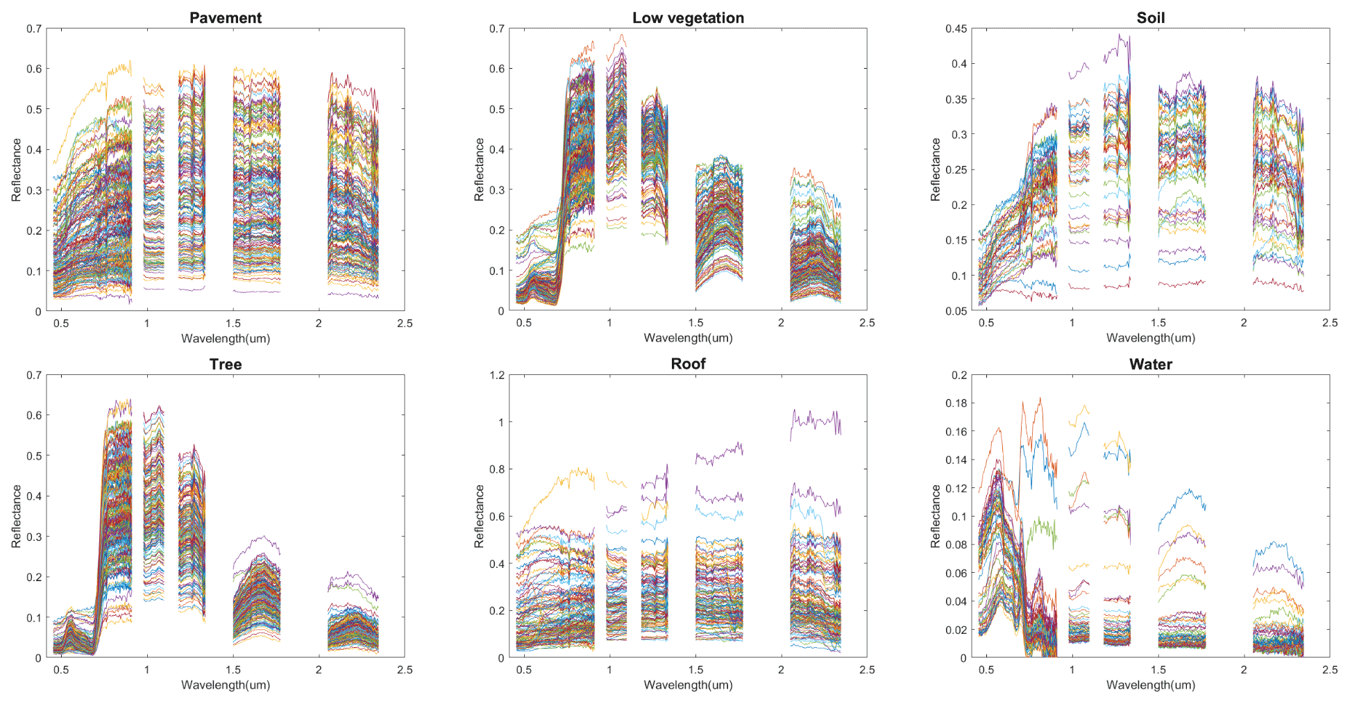
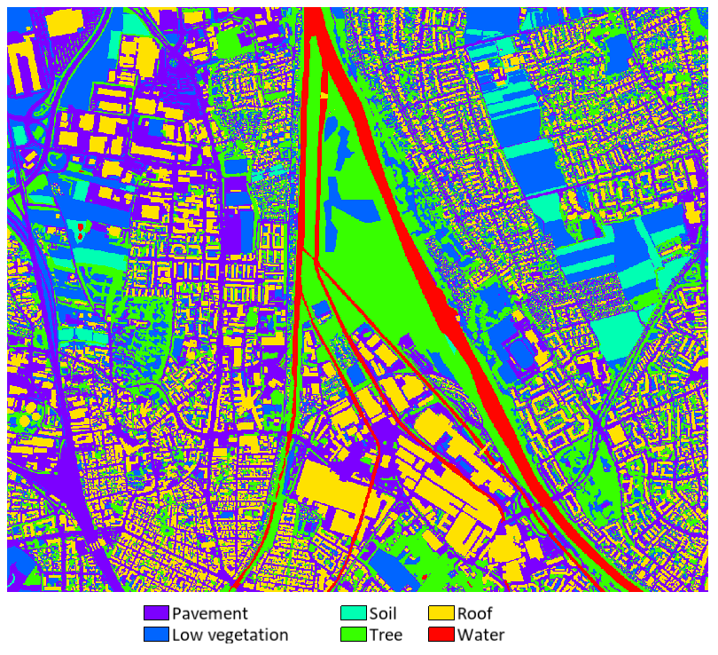
Figure 5 The manually delineated land cover composition of the sub1 region based on the DLR 3K image.

2.6 Manually labelled data

Three subregions were selected to be labelled, and their location in the original image is shown in Fig. 3. A spectral library of the most dominant urban materials for the HySpex hyperspectral image was constructed by manually chosen pure pixels throughout the subregions of the HySpex data. In total, the spectral library contains 859 endmember spectra with 181 spectra being pavement, 211 spectra being low vegetation, 49 spectra being soil, 210 spectra being tree, 134 spectra being roof, and 74 spectra being water. The spectra for each land cover class are shown in Fig. 4. To obtain sub-pixel level information of mixed pixels for the unmixing task, the land cover mapping products of six classes, namely, pavement, low vegetation, soil, tree, roof, and water, were manually delineated across the 0.2 m DLR 3K image. The elaborately produced land cover maps of the three subregions are presented in Figs. 5–7. The ground-truth maps can be used to generate reference abundances for quantitative evaluations of the hyperspectral unmixing task.

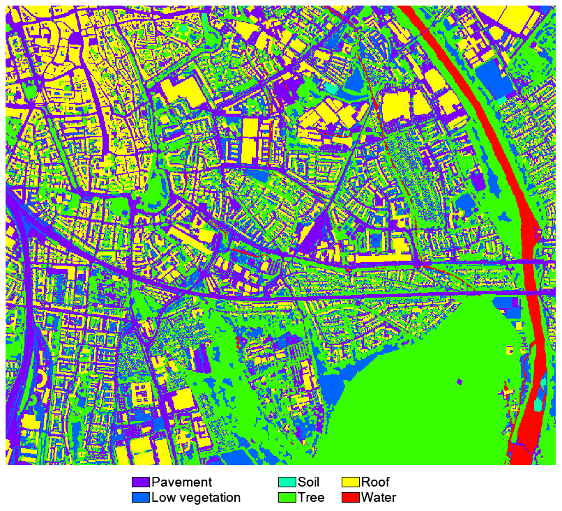
Figure 6 The manually delineated land cover composition of the sub2 region based on the DLR 3K image.

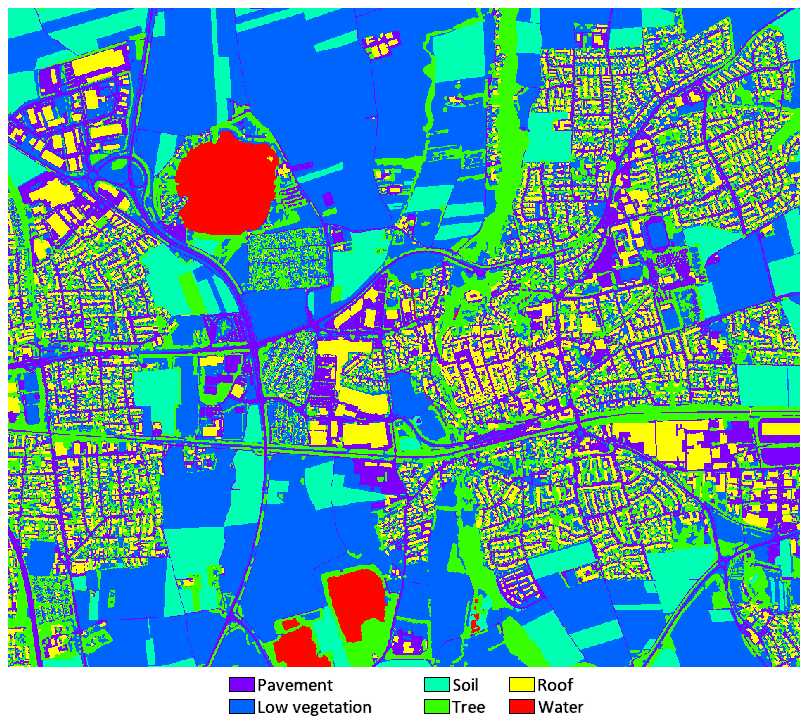
Figure 7 The manually delineated land cover composition of the sub3 region based on the DLR 3K image.

2.7 Data summary

The data components of MDAS are listed in Table 2. They are a Sentinel-1 SAR image, a Sentinel-2 multispectral image, a DLR 3K DSM, and a HySpex hyperspectral image. These four components are data sets collected from operating missions. Besides this, MDAS includes some HySpex-based simulated data. The S2eteS_S2 is a simulation of Sentinel-2 image in terms of the spatial and spectral characteristics. The EeteS_EnMAP_10 imitates the spectral bands of EnMAP, yet with a 10 m GSD. The EeteS_EnMAP_30 imitates both the spectral bands and 30 m GSD of EnMAP. Meanwhile, the simulation of EnMAP includes additionally the effects of instrumental and environmental parameters. At last, MDAS also has components which can be used as ground reference. They are OSM GIS maps and manually labelled endmember and land cover maps.

Table 2 This table lists data components of MDAS.

3 Experiments

3.1 Super-resolution

3.1.1 Selected algorithms

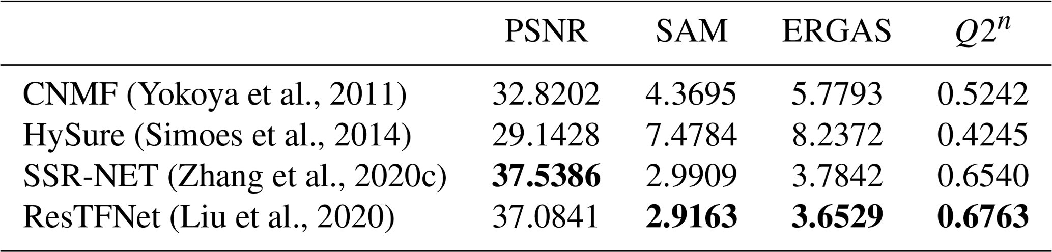
In this paper, we select representative super-resolution algorithms among the literature and demonstrate their performance on our MDAS data set. The experiment results can be treated as the baseline for further studies. Our selection of algorithms are based on two papers, Yokoya et al. (2017) and Zhang et al. (2020c), as both studies carry out comprehensive comparative experiments and publish their source codes. Yokoya et al. (2017) implements 10 conventional algorithms, tests them on eight data sets, and evaluates the performance with four metrics. Based on the 32 evaluations (four metrics on eight data sets) in Yokoya et al. (2017), we selected HySure (Simoes et al., 2014) and CNMF (Yokoya et al., 2011), since they most frequently rank the first place, respectively, 13 and 8 times. Zhang et al. (2020c) implements six deep learning models, tests on six data sets, and applies four evaluation metrics. We choose SSR-NET (Zhang et al., 2020c) and ResTFNet (Liu et al., 2020) as they rank the first place for 18 and 6 times. In the following, we briefly recap the selected algorithms. CNMF (Yokoya et al., 2011) applies non-negative matrix factorization on both hyperspectral and multispectral images so that hyperspectral endmembers and multispectral abundance map are extracted and further fused to achieve an image of high-resolution in both spectral and spatial domain. HySure (Simoes et al., 2014) attempts to fuse hyperspectral and multispectral images by fitting both of them to a latent representation. To do so, they optimize two quadratic terms that fit the two images to the latent representation and a regularizer to preserve edges. Liu et al. (2020) proposes a two-stream convolutional neural network (CNN) whose two branches extract representation from hyperspectral and multispectral images, respectively, fuse high-level representations at a late stage, and recover an image of high spectral and spatial resolution with a reconstruction loss. Zhang et al. (2020c) trains a CNN to accomplish super-resolution by a loss function of three terms. These terms represent differences on spectral edges, spatial edges, and the data. Their training applies corresponding image patches of hyperspectral image, multispectral image, and the targeted image of high spectral and spatial resolution.

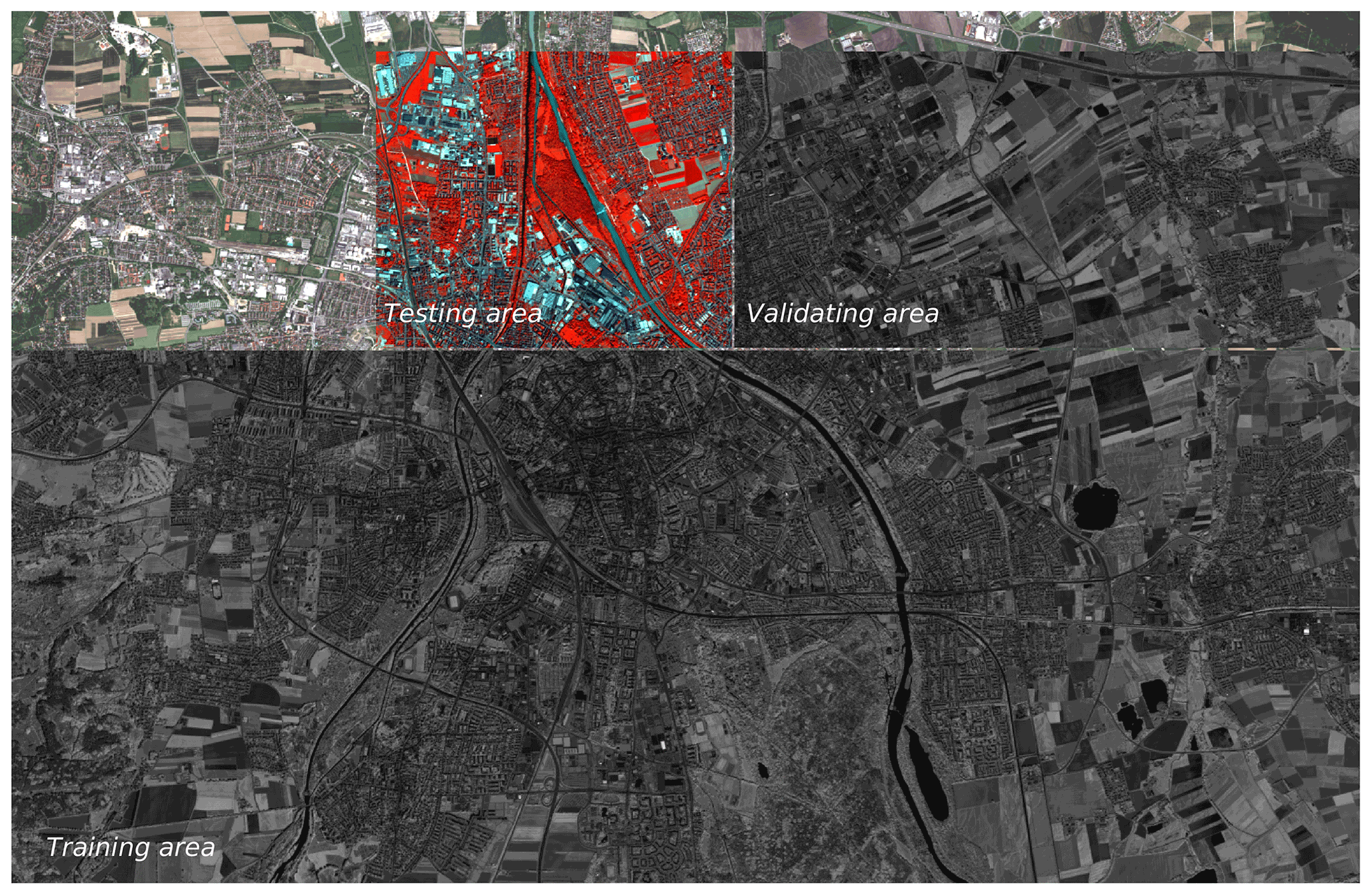
Figure 8 This figure demonstrates the data of the three regions that are used for the training, validating, and testing of the super-resolution algorithms. The visualization is based on EeteS simulated Sentinel-2 image. The background, testing area, validating area, and training area are visualized by R–G–B (663–560–492 nm), IR–G–B (842–560–492 nm), IR (842 nm), and IR (842 nm), respectively. IR is short for infrared.

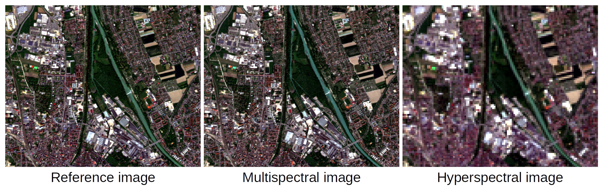
Figure 9 Visualizations of reference image, multispectral image, and hyperspectral image for the testing area.

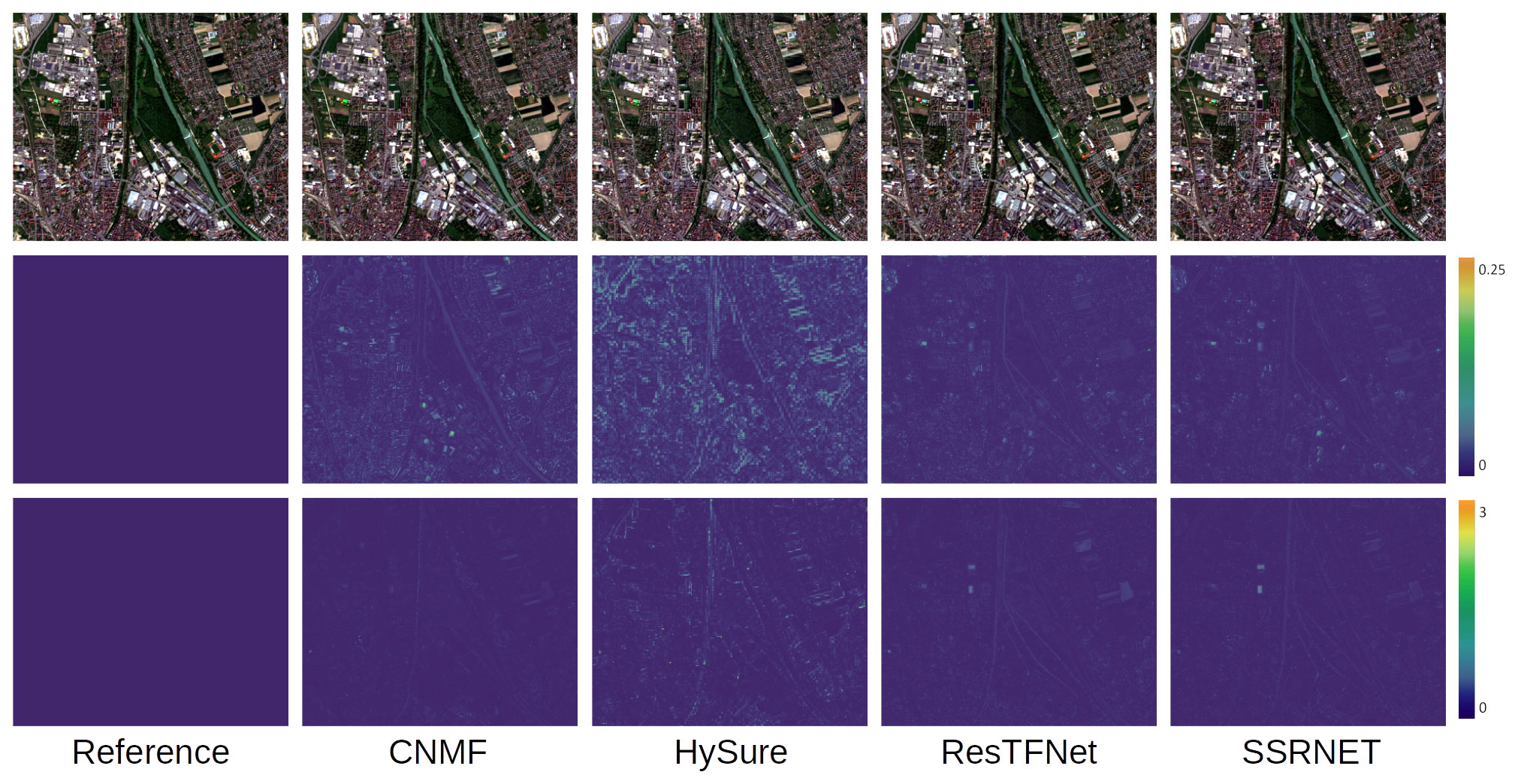
Figure 10 Visualizations of super-resolution results. The first row demonstrates RGB images composed of bands of 652, 553, and 450 nm. The second row demonstrates the rooted squared error between the reference and fusion results. The third row demonstrates the angle differences between the reference and fusion results.

Yokoya et al., 2011Simoes et al., 2014Zhang et al., 2020cLiu et al., 2020

Table 3 Quantitative assessment of super-resolution algorithms. The best results are shown in bold font.

3.1.2 Evaluation metrics

For quantitative evaluations, we implement four metrics to assess the super-resolution results, namely, PSNR, SAM, ERGAS, and Q2ⁿ. PSNR evaluates the spatial reconstruction of each band. We assess our experiments with an averaged PSNR over all bands. SAM is widely used to demonstrate the quality of spectral information via calculating the angle differences. ERGAS is a modified version of mean squared error that globally assesses the quality of data reconstruction. At last, Q2ⁿ aims to qualify spectral and spatial distortions. For more details about the four metrics, please refer to Yokoya et al. (2017).

Table 4 Quantitative assessment of unmixing algorithms for the sub1 region.

Table 5 Quantitative assessment of unmixing algorithms for the sub2 region.

3.1.3 Experiment setting

To train the algorithms, as shown in Fig. 8, we select three areas for training, validating, and testing the algorithms. This setting is required by the two deep learning models, SSR-NET and ResTFNet. Since HySure and CNMF do not require training with ground reference data, they work directly with data of the testing area.

On the aspect of data, we utilize the spatially simulated 10 m GSD hyperspectral image as the reference data, which have high spatial and high spectral resolution. The low spatial and high spectral resolution image is the spatially simulated 30 m GSD hyperspectral image. The high spatial and low spectral resolution image is the spectrally simulated 10 m multispectral image. Figure 9 visualizes these three images, and the details of simulations are introduced in Sect. 2.3.

The implementation of the deep learning models is based on the codes introduced in Zhang et al. (2020c), within PyTorch framework. The number of epochs is 10 000. The optimizer is Adam with a learning rate of 10⁻⁴. The best model is saved along the training procedure, based on the assessment on the validation data after each epoch. The codes of the shallow models are accessible with Yokoya et al. (2017).

3.1.4 Experiment results and visualization

Table 3 shows the quantitative measures for the performance of the selected four super-resolution algorithms. ResTFNet has the best performance among them by ranking the first for three indications. The two deep learning models significantly outperform the other two conventional algorithms, at the cost of requiring dramatically more data for training models. Figure 10 visualizes the super-resolution results, images of root squared error, and images of angle differences. For both root squared error and angle differences, HySure has the largest error. The two deep learning models have smaller errors compared to the two conventional algorithms. It is interesting to point out that, in terms of angle differences, CNMF seems to outperform the two deep models.

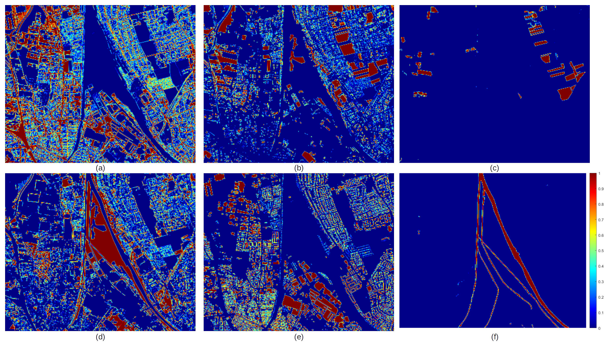
Figure 11 Ground truth of abundance maps of the sub1 region of the EeteS_EnMAP_10 data. (a) Pavement. (b) Low vegetation. (c) Soil. (d) Tree. (e) Roof. (f) Water.

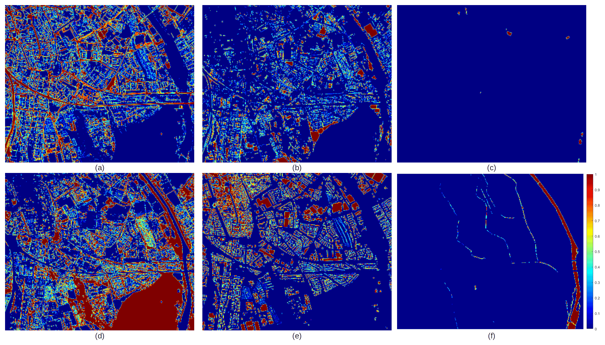
Figure 12 Ground truth of abundance maps of the sub2 region of the EeteS_EnMAP_10 data. (a) Pavement. (b) Low vegetation. (c) Soil. (d) Tree. (e) Roof. (f) Water.

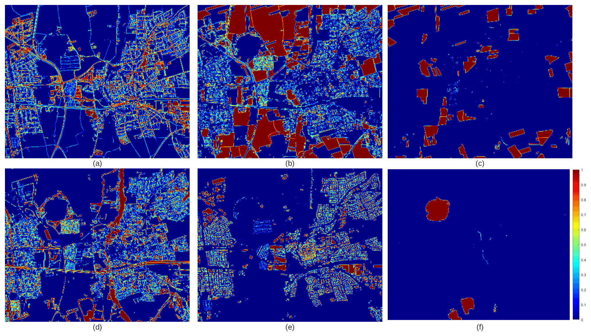
Figure 13 Ground truth of abundance maps of the sub3 region of the EeteS_EnMAP_10 data. (a) Pavement. (b) Low vegetation. (c) Soil. (d) Tree. (e) Roof. (f) Water.

3.2 Hyperspectral unmixing

3.2.1 Ground truth

In the experiments, the endmember spectra shown in Fig. 4 were used by methods which need a spectral library as prior knowledge. The abundance ground truth for quantitative evaluation of unmixing performance was generated from the land cover map shown in Figs. 5–7. The generated abundance maps of the three subsets are displayed in Figs. 11–13.

Table 6 Quantitative assessment of unmixing algorithms for the sub3 region.

3.2.2 Selected algorithms

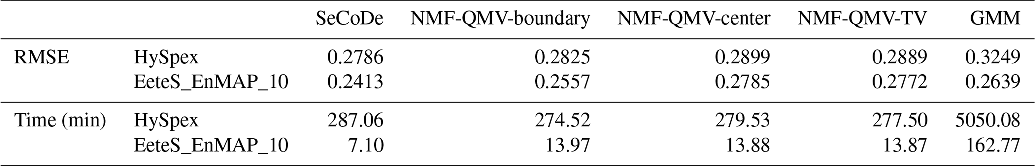
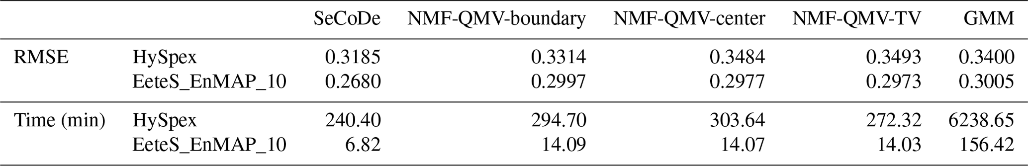
There are several categories of unmixing algorithms (Hong et al., 2021a). In this paper, we tested the performance of algorithms on the generated dataset that belong to these three categories: (1) unmixing methods that do not need the spectral library as prior knowledge and do not consider the intra-class spectral variability; (2) unmixing methods that do not need the spectral library as prior knowledge and consider the intra-class spectral variability; and (3) assume that there is a spectral library of pure spectra representing endmember variability for a set of endmember classes and unmix the image with the library. The NMF-QMV algorithm (Zhuang et al., 2019), SeCoDe algorithm (Yao et al., 2021) and GMM algorithm (Zhou et al., 2020) are selected as the representative algorithms that belong to the three categories, respectively. NMF-QMV conducts unmixing via introducing three kinds of well-known minimum volume regularization terms, referred to as boundary, center, and total variance (TV) into the nonnegative matrix factorization framework, in which the regularization parameter between the data-fitting term and the regularization term is selected automatically. SeCoDe jointly captures the spatial–spectral information of hyperspectral image in a tensor-based fashion, in which the convolutional operation is employed to locally model the spatial relation between neighbouring pixels by spectral bundles that represent spectral variability (Hong et al., 2019a). Experiments on three hyperspectral datasets showed that SeCoDe outperformed other state-of-the-art unmixing algorithms. GMM assumes that the endmembers for each pixel are sampled from probability distributions, hence the pixels as linear combinations of these endmembers also follow the distribution. It works by using Gaussian mixture model for distributions and unmixing pixels based on the estimated distribution parameters. Experiments on both synthetic and real hyperspectral images showed that GMM performed best among the distribution-based methods and achieved comparable unmixing accuracy to set-based methods without the need for library reduction; it may also be more stable across datasets.

3.2.3 Evaluation metric

The spectral angle distance (SAD) and root mean square error (RMSE) are two most widely used evaluation metrics for unmixing (Liu and Zhu, 2020). Since the tested methods contain the method that uses spectral library as prior information, only RMSE between the estimated abundance and the ground truth abundance is employed for quantitative evaluation. A smaller RMSE value means better performance.

3.2.4 Experiment setting

We tested the selected algorithms on the three subsets of HySpex data and the EeteS_EnMAP_10 data. For NMF-QMV, the three regularization terms, boundary, centre, and TV are chosen separately, and no other parameter needs to set. For SeCoDe, there are three regularization parameters (α,β, and γ) that need to be manually adjusted. We conducted parameter analysis on the sub1 region of EeteS_EnMAP_10 data, and the parameter combination that produces the minimum mean RMSE value is α=0.3, β=0.01, and γ=3. This parameter combination was directly used for other images. For GMM, no parameter was manually set. All the algorithms were implemented in Matlab on a PC with Intel Core i7-6700 CPU and 64 GB memory.

3.2.5 Results

Tables 4–6 show the quantitative assessments for the performance of the selected unmixing algorithms. For both of the HySpex and EnMAP dataset, SeCoDe has the best performance in terms of RMSE. Regarding the computation time, although SeCode is the most efficient, it needs extra time to select the best parameters, while the NMF-QMV-based methods do not need parameter tuning. GMM is the most time-consuming method. The efficiency of all methods decreased largely when the size of the image increased.

3.3 Multimodal land cover classification

3.3.1 Experimental setup

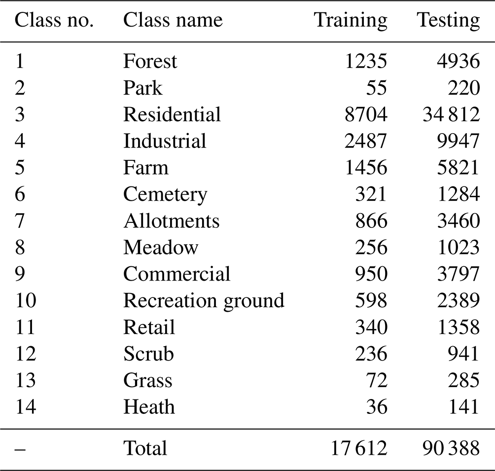
We selected pixel-wise classification as a potential application to evaluate the performance of different modality combinations for the land cover mapping task on the Augsburg dataset. The classification performance is quantitatively shown in terms of three common indices, i.e. overall accuracy (OA), average accuracy (AA), and kappa coefficient (κ), using canonical correlations forest (CCF) classifier (Rainforth and Wood, 2015). We choose the sub area the same as Fig. 5 to conduct our experiments. The sample statistics are summarized in Table 7, in which 20 % samples were randomly selected as the training set.

Table 7 This table lists category information of the investigated dataset.

In this task, we investigate the classification performance with the use of different combinations of RS modalities. They include the following:

• single modality, e.g. HS, MS, SAR, DSM;

• two modalities, e.g. HS-MS, HS-SAR, HS-DSM, MS-SAR, MS-DSM, SAR-DSM;

• three modalities, e.g. HS-MS-SAR, HS-MS-DSM, HS-SAR-DSM, MS-SAR-DSM;

• four modalities, e.g. HS-MS-SAR-DSM.

3.3.2 Results and discussion

Table 8 lists the classification results of all possible combinations of modalities on the to-be-released multimodal benchmark dataset, i.e. Augsburg. Moreover, only using HS or MS data is apt to obtain better classification results than SAR or DSM. The input with two modalities (even though SAR plus DSM) obviously yields a performance improvement compared to the single modality. Similarly, the use of three modalities achieves a better result on the basis of two modalities. As expected, the classification accuracies by using all modalities are superior to those by using single modality, two modalities, and three modalities, achieving the best classification performance. This can demonstrate the necessity and important values to investigate and build such a multimodal benchmark dataset in the RS community, which can help us break the performance bottleneck in many single-modality-oriented applications and meanwhile point out the future research direction.

Here, we only show the baseline results as a reference by using the CCF classifier directly conducted on the original RS data, in order to provide a larger space to the subsequent potential researchers who are interested in the topics related to multimodal feature extraction and classification for RS data. In addition, we also visualize the corresponding classification maps, as illustrated in Fig. 14, where there is a basically similar trend with quantitative results.

Table 8 Classification results of different modality combinations using the CCF classifier on the investigated dataset. The best results are shown in bold font.

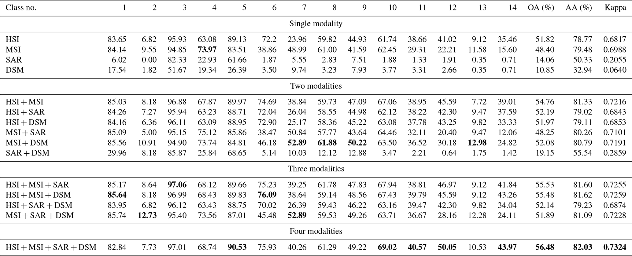
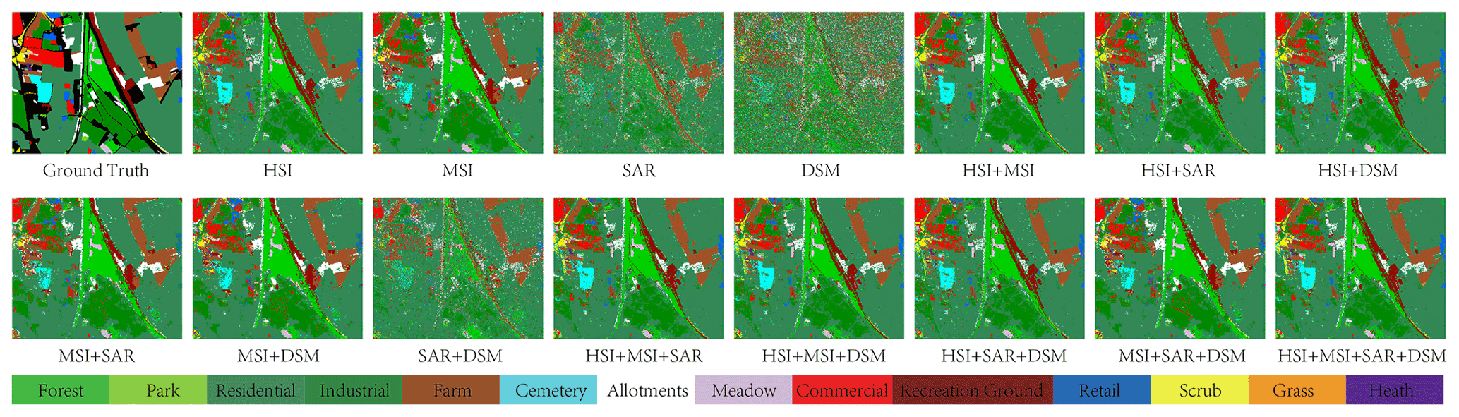
Figure 14 Visualization of classification results obtained by the CCF classifier using different modalities.

4 Code and data availability

The data are accessible at https://doi.org/10.14459/2022mp1657312 with a CC BY-SA 4.0 license (Hu et al., 2022a), and the code (including the pre-trained models) is at https://doi.org/10.5281/zenodo.7428215 (Hu et al., 2022b). Also, the live repository is available at https://github.com/zhu-xlab/augsburg_Multimodal_Data_Set_MDaS (last access: 2 January 2023).

5 Conclusions

In this paper, we contributed to the community a new multimodal benchmark data set, MDAS, at the scene of Augsburg, Germany. It includes five different data modalities, which are SAR, multispectral image, hyperspectral image, DSM, and GIS data. All data modalities were collected on the same day, 7 May 2018. Experienced experts put a lot of effort in the collection and preparation of the data set to ensure a high quality. MDAS not only provides new benchmark data for current data fusion applications, but some of its components enrich data options for applications of single data source, such as the DSM and hyperspectral images. Additionally, the multiple modalities make it possible to explore different combinations. Besides the data itself, we contribute by demonstrating the performance of state-of-the-art algorithms on MDAS in terms of super-resolution, unmixing, and land cover classification. These experiment results provide baselines for further studies that use MDAS, including but not limited to multimodal data fusion, the automatic design of neural architectures and ML pipelines (NAS and AutoML) for multimodal data, multi-fidelity problems (e.g. considering multi and hyperspectral data as different resolutions), domain adaption (e.g. training a model on this high-quality data set and deploying it into a new region), and transfer learning across modalities, among many others.