Multi-year, spatially extensive, watershed-scale synoptic stream chemistry and water quality conditions for six permafrost-underlain Arctic watersheds

Repeated sampling of spatially distributed river chemistry can be used to assess the location, scale, and persistence of carbon and nutrient contributions to watershed exports. Here, we provide a comprehensive set of water chemistry measurements and ecohydrological metrics describing the biogeochemical conditions of permafrost-affected Arctic watersheds. These data were collected in watershed-wide synoptic campaigns in six stream networks across northern Alaska. Three watersheds are associated with the Arctic Long-Term Ecological Research site at Toolik Field Station (TFS), which were sampled seasonally each June and August from 2016 to 2018. Three watersheds were associated with the National Park Service (NPS) of Alaska and the U.S. Geological Survey (USGS) and were sampled annually from 2015 to 2019. Extensive water chemistry characterization included carbon species, dissolved nutrients, and major ions. The objective of the sampling designs and data acquisition was to characterize terrestrial–aquatic linkages and processing of material in stream networks. The data allow estimation of novel ecohydrological metrics that describe the dominant location, scale, and overall persistence of ecosystem processes in continuous permafrost. These metrics are (1) subcatchment leverage, (2) variance collapse, and (3) spatial persistence. Raw data are available at the National Park Service Integrated Resource Management Applications portal (O'Donnell et al., 2021, https://doi.org/10.5066/P9SBK2DZ) and within the Environmental Data Initiative (Abbott, 2021, https://doi.org/10.6073/pasta/258a44fb9055163dd4dd4371b9dce945).

1 Introduction

Watershed chemistry studies – like all ecosystem studies – involve trade-offs between sampling extent (i.e., how much area is observed) and spatiotemporal grain (i.e., the resolution of observations in space and time) (Abbott et al., 2018; Burns et al., 2019; Ward et al., 2019). Initial assessments are typically performed at the plot (terrestrial studies, <1 to 100 m²) (Keller et al., 2007; Prager et al., 2017) or reach scales (stream studies, 100–1000 m), where replicated observations and manipulations can be made (Kling et al., 2000; Docherty et al., 2018). Trade-offs between extent and grain are especially apparent in remote settings such as the Arctic, where logistical constraints and high operational costs often force researchers to choose among these sampling approaches (Abbott et al., 2021). While these intensive studies are crucial to identifying the underlying processes controlling solute transport and transformations, it is challenging to scale up plot-level observations to the watershed, regional, or continental levels (Wiens, 1989; Thrush et al., 1997; Helton et al., 2012). Likewise, large-scale observations sensed remotely from aircraft or satellites often cannot identify the processes behind the regional to continental patterns they reveal (Newman et al., 2019; Shiklomanov et al., 2019). Bridging small- and large-scale observations is complicated by both spatial heterogeneity and temporal variation, as mosaics of diverse ecosystem patches evolve in space and time (Bernhardt et al., 2017; Pinay et al., 2015; Abbott et al., 2016). Consequently, mechanisms that are observed at the plot or regional levels may not reconcile (Kareiva and Andersen, 1988) because connectivity among patches can create emergent patterns and processes (Sivapalan, 2003; McDonnell et al., 2007; Covino, 2017). To understand and predict ecosystem behavior in the Anthropocene, we need to observe how biogeochemical patterns are produced and propagate across scales. Here, we describe a medium-scale watershed chemistry dataset that includes spatially distributed hydrological, ecological, and geochemical properties. Using a synoptic experimental design, we measured these parameters across medium-scale watersheds (<1 to >1000 km²) multiple times over several years. We hope this dataset will help bridge the gap between plot-level and regional investigation of ecosystem change in the permafrost zone.

Most water chemistry and flow assessments conducted in the Arctic and elsewhere are based on observations at river outlets (McClelland et al., 2006, 2007; Tank et al., 2016; Toohey et al., 2016; Shogren et al., 2020; Zarnetske et al., 2018). The flow of water integrates biogeochemical signals, such that river chemistry at the watershed outlet contains information about both terrestrial and aquatic biogeochemical processes that occurred upstream in the network (Temnerud et al., 2010; Vonk et al., 2019; Tank et al., 2020). Indeed, using sampling and monitoring approaches that capture the watershed outlet response over time has logistic and safety advantages for site access. Further, the recent application of novel sensor technology has enabled high-frequency watershed-scale studies (Shogren et al., 2021; Ruhala and Zarnetske, 2017; Khamis et al., 2021). For example, the paired high-frequency flow and a limited set of chemical properties for the watersheds in this data paper are available at the Arctic Data Center (Zarnetske et al., 2020b, c, a). While these watershed outlet measurements can provide insight into possible upstream and upslope processes (Laudon et al., 2017; Shogren et al., 2021; Moatar et al., 2017), they often do not diagnose primary drivers of lateral transport of materials (Burns et al., 2019; Appling et al., 2018; Temnerud et al., 2010; Hoffman et al., 2013; Collier et al., 2018). These large-scale measurements are the result of variable inputs which are buffered and blurred as multiple spatiotemporal signals are mixed and propagated through the surface and subsurface network (Creed et al., 2015; Abbott et al., 2018; Kolbe et al., 2019). To identify the processes behind those signals, we need to venture into the headwaters, extending our observations into smaller subcatchments that match the spatial scale of mechanisms controlling carbon and nutrient uptake and release (Shogren et al., 2019; Gu et al., 2021; Abbott et al., 2017).

Spatially extensive or “synoptic” sampling frameworks, such as contained in this data paper, provide multi-scale information about the source of signals across the entire watershed network, creating a direct complement to watershed outlet monitoring. With a synoptic sampling design, researchers can capture the spatial extent of nested subcatchments and therefore assess terrestrial–aquatic transfer of material and stream network processing (Abbott et al., 2018; Shogren et al., 2019; Gu et al., 2021). Though synoptic campaigns are logistically challenging (Yi et al., 2010; Abbott et al., 2021; Rodríguez-Cardona et al., 2020), the high-resolution spatial snapshot they generate allows empirical assessment of biogeochemical signals at intermediate spatial scales (Abbott et al., 2018; Shogren et al., 2019; McGuire et al., 2014). In recent years, synoptic campaigns have focused on solute distribution in temperate river systems (Gardner and McGlynn, 2009; McGuire et al., 2014; Byrne et al., 2017; Abbott et al., 2018; Dupas et al., 2019). While there have been fewer synoptic campaigns in permafrost systems (Kling et al., 2000; Bowden, 2013; Shogren et al., 2020; Abbott et al., 2015, 2021; Lamhonwah et al., 2017), their application presents an opportunity to characterize the fate of carbon and nutrients in a rapidly changing Arctic, creating multi-scale targets for the Earth system models used for predicting environmental change (Collier et al., 2018; Koven et al., 2015; Turetsky et al., 2020; Vonk et al., 2015). Because permafrost degradation is triggering both large-scale deepening of the active layer and discrete permafrost collapse (thermokarst) features (Gao et al., 2021; Turetsky et al., 2020; Farquharson et al., 2019), synoptic snapshots could be invaluable in detecting the degree, location, and type of climate response. Therefore, measuring the spatial distribution of water chemistry in high-latitude river networks could advance understanding of permafrost ecosystems and improve estimates of ecosystem feedbacks to climate change (Bring et al., 2016; Wrona et al., 2016; Schuur et al., 2015; Mu et al., 2020).

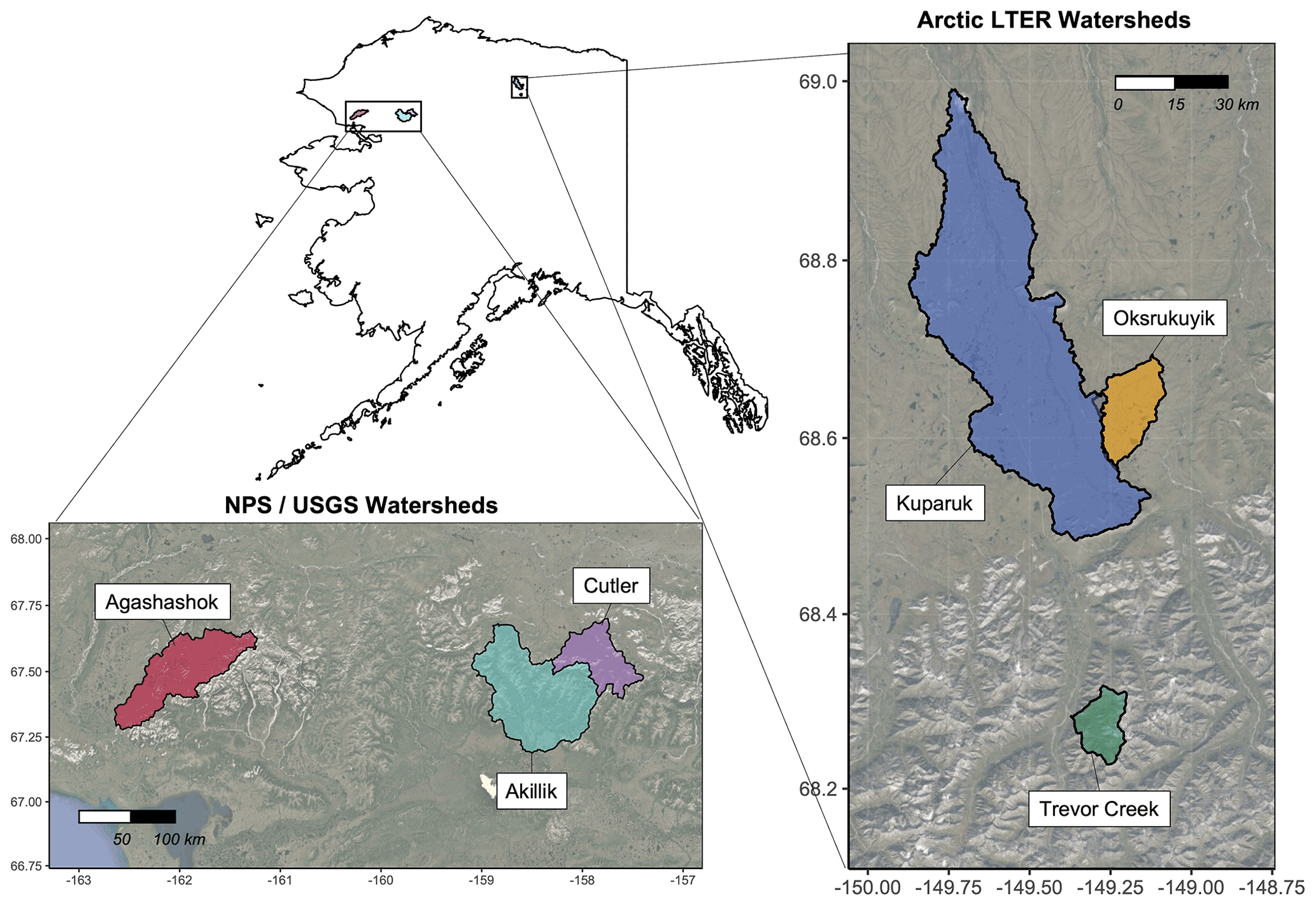
Figure 1 Regions of northern Alaska associated with the Arctic Long-Term Ecological Research site at Toolik Field Station (TFS) and National Park Service (NPS) and U.S. Geological Survey (USGS) watersheds. Map created in R Studio (version 1.2.1335) with base imagery from ESRI and © Google Earth (version 7.3.3.7786).

The datasets presented here were derived from repeated synoptic samplings in six Arctic watersheds in northern Alaska occurring on three distinct high-latitude ecosystem types: Arctic tundra, boreal forest, and Alpine tundra (Fig. 1). In this paper, we illustrate the utility of such data via a set of initial watershed chemistry analyses for ecologically significant reactive solutes including dissolved organic carbon (DOC), nitrogen (e.g., nitrate, N-${{\mathrm{NO}}_{\mathrm{3}}}^{-}$; ammonium, N-${{\mathrm{NH}}_{\mathrm{4}}}^{+}$; dissolved organic nitrogen, DON; total dissolved nitrogen, TDN), phosphorous (soluble reactive phosphorus, SRP; total dissolved phosphorus, TDP), and a suite of geochemically significant anions and cations (e.g., calcium, Ca²⁺; total iron, Fe; dissolved silica, DSi; see Table 1 for full list of analytes). In addition, we use these datasets to introduce simple metrics for biogeochemical solutes: variance collapse, subcatchment leverage, and spatial persistence (Abbott et al., 2018; Shogren et al., 2019; Gu et al., 2021; Dupas et al., 2019; Frei et al., 2020). These new metrics seek to extract information more fully from rich spatiotemporal water chemistry datasets. Specifically, these metrics characterize what spatial scale is the most relevant in explaining terrestrial–aquatic material flux, how much influence or leverage each sampling site has on the watershed budget, and whether individual samplings are adequate to capture temporal variation. In this light, synoptic sampling frameworks provide robust information about how to scale plot- and reach-level observations while also providing a multi-scale target for remotely sensed data and numerical models. Ultimately, the information gleaned from these metrics is desired by a range of disciplines from ecologists to natural resource managers.

Table 1 Summary of site characteristics for the watersheds where synoptic samplings were conducted. The descriptions are considered representative of the major landform types within the TFS and NPS/USGS watersheds.

First, we use subcatchment leverage to identify nested areas within the network that exert a disproportionate influence on flux at the watershed outflow (Abbott et al., 2018; Shogren et al., 2019). Subcatchment leverage can be interpreted as the contribution of the subcatchment to watershed mass flux where the value can be negative (indicating the subcatchment has lower areal flux than the outlet, decreasing watershed flux), positive (indicating the subcatchment has higher areal flux than the outlet, a net increase in flux), or zero (no influence because it is the same as the outlet). Estimating leverage allows identification of specific subcatchments with disproportionate influence on material export, defined here as high leverage. Subcatchments with high leverage behave as a strong source or sink within the watershed network, strongly influencing the resulting concentrations at the outflow, and can be selected as sites for further mechanistic study or monitoring. Likewise, the direction and magnitude of leverage averaged across the entire watershed contain information about net solute removal and production in the stream network (Shogren et al., 2019). For example, if the mean leverage for the watershed is above zero, this indicates there are more solute sources than can be accounted for at the watershed outlet, implying there has been solute removal during transport through the network. Second, we examine what spatial extent or patch size controls solute production and removal by identifying thresholds of concentration variance collapse (Abbott et al., 2018). We generally expect the amplitude of solute variability to decrease moving downstream from headwaters to larger systems (Creed et al., 2015) with greater variability among headwaters, whereas downstream reaches are less likely to have extremely high or low concentrations because they integrate multiple upstream source or sink processes (Wolock et al., 1997; Temnerud and Bishop, 2005; Burt and Pinay, 2005; Abbott et al., 2017). Therefore, the size of nutrient sources and sinks in the landscape can be assessed by the spatial scale of the variance collapse of concentration among watershed reaches (Abbott et al., 2018; Shogren et al., 2019). The threshold of variance collapse is similar to the elementary representative area concept (Zimmer et al., 2013, p. 20), where the threshold represents the spatial scale at which landscape “patches” or processes throughout the watershed network that produce and remove solutes are effectively integrated. Lastly, the spatial persistence metric can be used to assess whether a given site is representative (i.e., the same pattern continues through time), or if patches restructure in space between sampling campaigns (i.e., reorganization of patches requires greater frequency in sampling) (Abbott et al., 2018; Dupas et al., 2019; Gu et al., 2021). Spatial persistence effectively quantifies the temporal representativeness of an instantaneous measurement at a given site, potentially indicating the type of process creating the patterns and informing future watershed study design and data analysis of extant data (Kling et al., 2000; Shogren et al., 2019).

2 Study location and design

2.1 Study watersheds

2.1.1 Arctic LTER sites at Toolik Field Station

The Arctic Long-Term Ecological Research (LTER) site based out of Toolik Field Station (TFS) is in the foothills of the Brooks Range on the North Slope of Alaska, USA (mean elevation 720 m). We conducted surveys in three watersheds near TFS: the Kuparuk River, Oksrukuyik Creek, and Trevor Creek. The three study watersheds were chosen because they spanned dominant circumarctic vegetation types, permafrost characteristics, and hydrologic conditions (Table 1). Further, the climate, morphology, and ecology of the sites and region have been previously described (Hobbie and Kling, 2014).

• The Kuparuk River (68.64816, −149.41152; Fig. 2a) is a meandering stream flowing through primarily tundra vegetation, located about 10 km northeast of TFS. The Kuparuk River includes a long-term monitoring site for the Arctic LTER, used as a site for ecological study and monitoring since 1979. From 1983–2016, the fourth-order reach of the Kuparuk River was used for a whole-stream fertilization study (Peterson et al., 1993; Slavik et al., 2004; Iannucci et al., 2021), where phosphorous (H₃PO₄) was continuously added to assess response to nutrient fertilization. As the Kuparuk River continues north, it meets a large aufeis (ice) field (Yoshikawa et al., 2007; Terry et al., 2020).

• Oksrukuyik Creek (68.68740, −149.095, Fig. 2b) is a clear-water, low-gradient stream meandering through primarily tundra landscape, with intermittent presence of stream-lake connectivity (Shogren et al., 2019). Oksrukuyik Creek is also an Arctic LTER long-term monitoring site, approximately 20 km northeast of TFS.

• Trevor Creek (68.28482, −149.350063, Fig. 2c) is a mountainous alpine stream, draining into the Atigun River watershed, located 30 km south of TFS. Trevor Creek drains primarily steep, rocky slopes with limited heath and willow vegetation. The majority of stream runoff is generated by precipitation and snowmelt.

As a result of long-term study and a sustained commitment to data stewardship, the Arctic LTER and TFS hosts an extensive catalogue of terrestrial, aquatic, and atmospheric data that are complementary to the data presented in this publication. For more information, please see the LTER data catalogue (https://arc-lter.ecosystems.mbl.edu/data-catalog, last access: 15 August 2021), in addition to the abiotic and biotic monitoring data from the TFS Spatial and Environmental Data Center (https://toolik.alaska.edu/edc/index.php, last access: 15 August 2021).

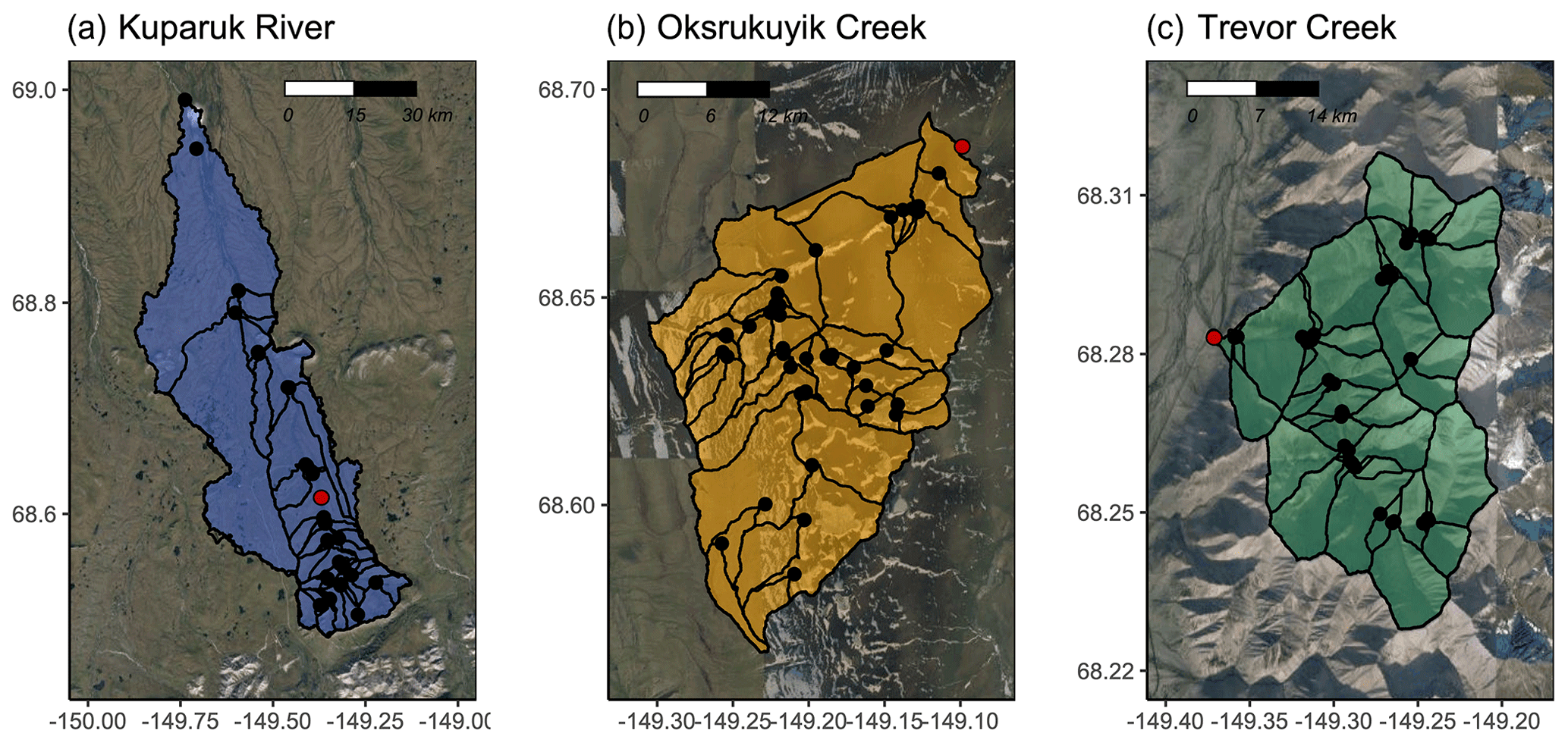
Figure 2 Synoptic sampling sites (black points) with subcatchment delineations from three watersheds related to the Arctic Long-Term Ecological Research site at Toolik Field Station (TFS) on the North Slope of Alaska. Study watersheds include the (a) Kuparuk River (blue), (b) Oksrukuyik Creek (orange), and (c) Trevor Creek (green). Scale bars in kilometers. The Arctic LTER monitoring stations are denoted by red points and described further in Shogren et al. (2021). Map created in R Studio (version 1.2.1335) with base imagery from ESRI and © Google Earth (version 7.3.3.7786).

2.1.2 National Park Service and U.S. Geological Survey sites

We also sampled three watersheds associated with the National Park Service (NPS) Arctic Inventory and Monitoring Network and a project funded by the U.S. Geological Survey's (USGS) Changing Arctic Ecosystem program. The Agashashok and Cutler River watersheds are within Noatak National Preserve, and the Akillik River watershed is within Kobuk Valley National Park. All three watersheds are situated near the northern extent of Alaska's boreal forest, where tree line is expanding (Suarez et al., 1999), and subcatchments vary in areal extent of forested versus tundra land cover. The study sites vary with respect to permafrost characteristics, including soil texture, ground ice content, and subsurface hydrology (O'Donnell et al., 2016). Evidence suggests stream chemistry varies across these watersheds, including the form, amount, and age of dissolved carbon (O'Donnell et al., 2020).

• The Cutler River (67.845, −158.316, Fig. 3a) flows north out of the Baird Mountains through gently rolling tundra into the upper Noatak River. The watershed is underlain by ice-rich glaciolacustrine deposits (O'Donnell et al., 2016), and soils tend to be organic-rich and poorly drained. Vegetation is dominated by moist acidic tundra and wet sedge meadows.

• The Akillik River (67.201, −158.572, Fig. 3b) flows south out of the Baird Mountains and into the Kobuk River downstream of the village of Ambler, Alaska. The river passes through alpine terrain in the headwaters before draining terrain comprised of ice-rich loess in the lower reaches. Vegetation is a mixture of boreal spruce forests and tundra.

• The Agashashok River (67.268, −162.636, Fig. 3c) is a braided, clearwater river that flows from the northeast to southwest into the lower Noatak River north of Kotzebue, Alaska. The headwaters drain rocky, alpine tundra terrain of the western Brooks Range. Downstream, the river drains broader valleys with a mixture of boreal spruce forest and tundra vegetation. The watershed is underlain by shallow bedrock, and permafrost is generally ice-poor (O'Donnell et al., 2016).

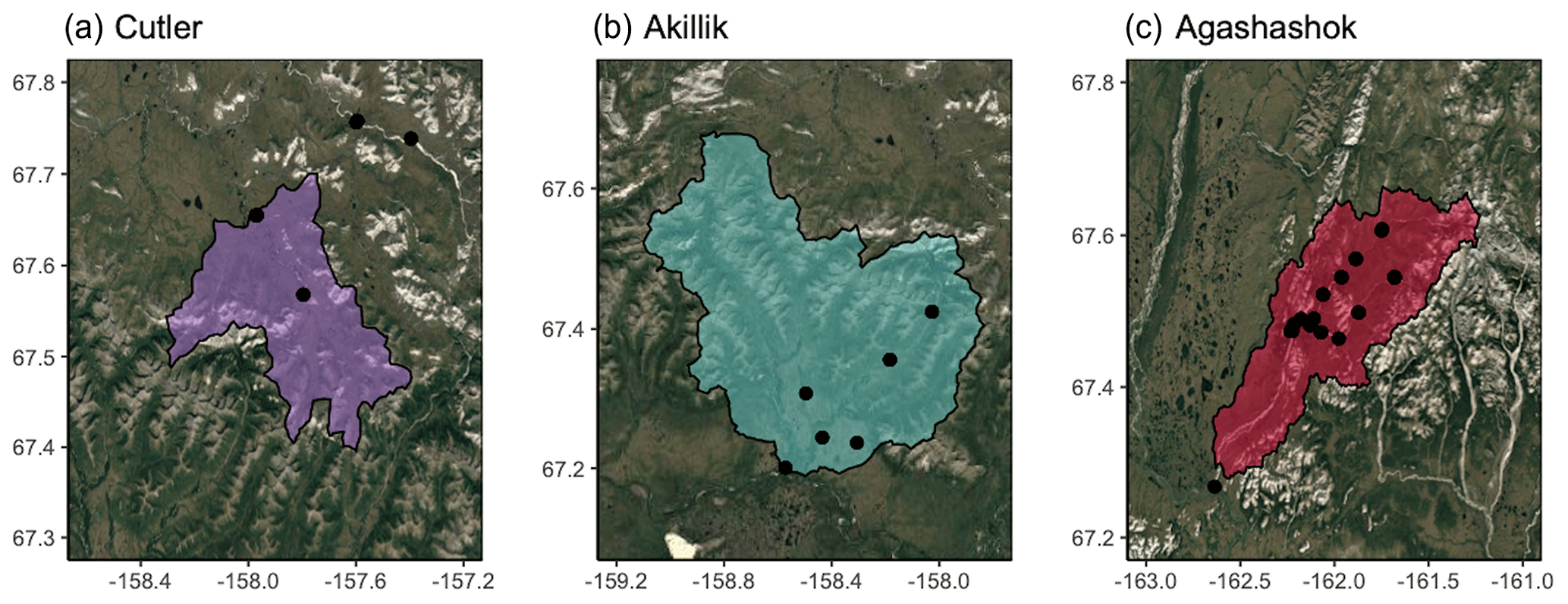
Figure 3 Synoptic sampling sites in three NPS/USGS watersheds. Study watersheds include the (a) Cutler, (b) Akillik, and (c) Agashashok rivers. Map created in R Studio (version 1.2.1335) with base imagery from ESRI and © Google Earth (version 7.3.3.7786).

2.2 Synoptic sampling campaign design

2.2.1 Arctic LTER sites

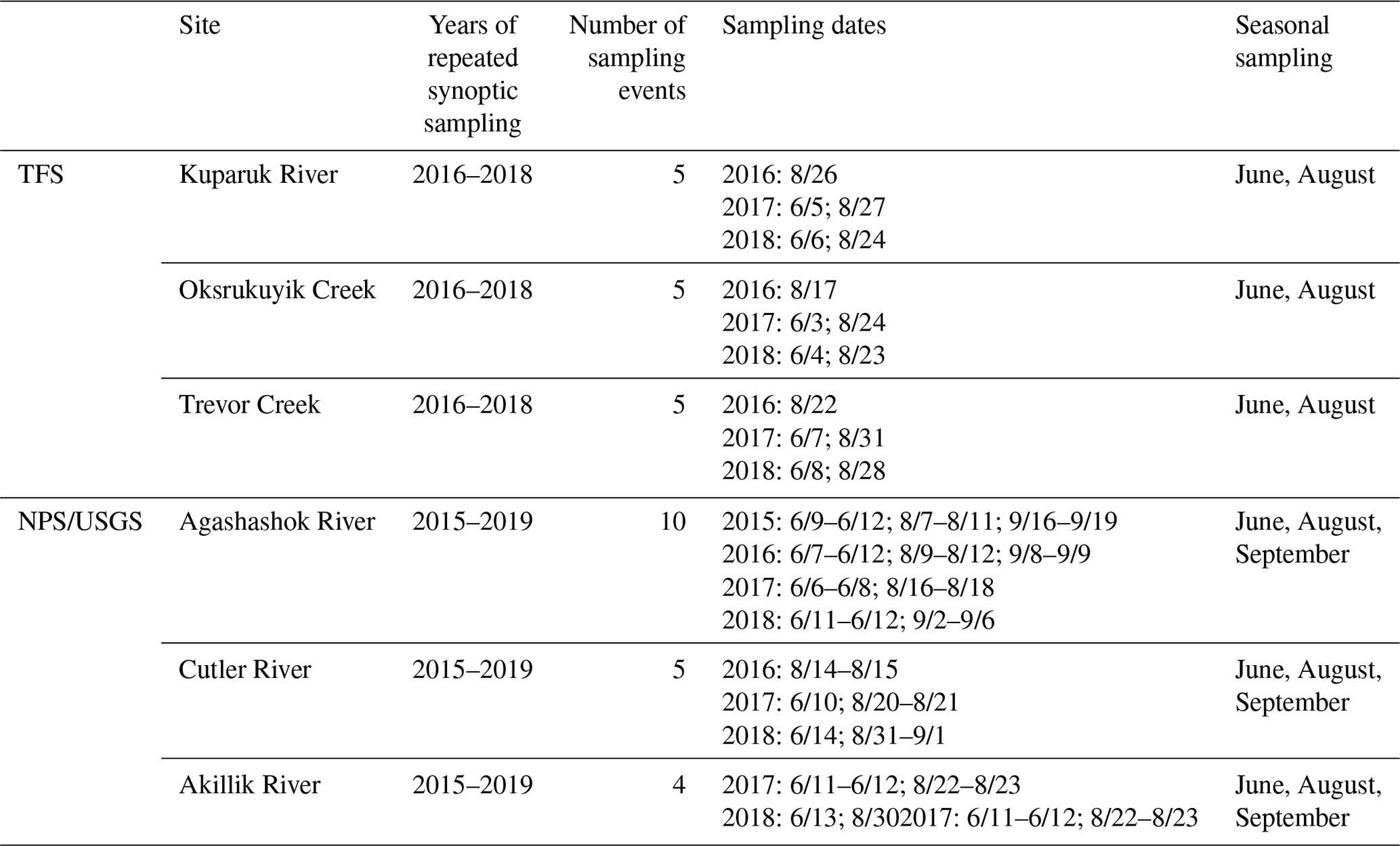
Our sampling of the TFS watershed networks was designed to capture 30–50 nested subcatchments within the Kuparuk River, as well as Oksrukuyik and Trevor creeks. Site selection was based primarily on (1) presence of flowing surface waters, (2) representation across varying subcatchment drainage areas, and (3) site accessibility. Often, we a priori chose sites located at subcatchment confluences, sampling both upstream locations and then downstream of river mixing. In each of the TFS watersheds, we performed five repeated synoptic campaigns, sampling each stream network in August 2016, June 2017, August 2017, June 2018, and August 2018 (exact dates in Table 2). We accessed sampling sites either on foot or by helicopter within a 6 h period.

Table 2 Description of the sampling campaign regimes, including dates for each campaign, for the TFS and NPS/USGS watersheds.

2.2.2 NPS/USGS sites

Sampling of the NPS/USGS watershed networks was designed to capture ∼5–10 subcatchments within the Agashashok, Cutler, and Akillik rivers. Sites were selected to span a gradient of size (subcatchment area, stream order), vegetation (forest vs. tundra), and permafrost characteristics (parent material, ground ice content). Due to variation in watershed aspect, streams also spanned a spatial gradient in permafrost ground temperatures, areal extent, and active layer thickness (Panda et al., 2016; Sjöberg et al., 2021). In addition to stream chemistry parameters, stream discharge was measured, and samples were collected to characterize stream biota (benthic biofilm, macroinvertebrates, and resident juvenile fish).

In each of the NPS/USGS watersheds, we performed 4–10 repeated synoptic campaigns, sampling each stream network in June, August, and September 2015; June, August, and September 2016; June and August 2017; and June and August or September 2018 (exact dates in Table 2). We accessed sampling sites by helicopter within a 24 to 96 h period.

3 Methods

3.1 Synoptic site characterization

3.1.1 Subcatchment delineation for drainage area

The location of each stream sampling site was recorded in a spreadsheet and imported into GIS software (ESRI ArcGIS v. 10.4). These sites served as starting points (“pour points”) from which watersheds and subcatchments were delineated following the general procedure described here: https://support.esri.com/en/technical-article/000012346 (last access: 1 May 2018). The following two digital elevation models (DEMs) were needed to cover the spatial distribution of the stream sampling sites and were used to create the necessary flow direction and flow accumulation layers: ArcticDEM from the Polar Geospatial Center (Porter et al., 2018) and ASTER GDEM v.2 (NASA/METI/AIST/Japan Space Systems and US/Japan ASTER Science Team, 2009). A Python script was written to iterate over the list of sample sites and execute the watershed delineation procedure.

3.1.2 Estimation of terrestrial catchment characteristics for TFS sites

We characterized the terrestrial environment of the TFS sites using remotely sensed data pertaining to the vegetation and topography of each subcatchment. For each subcatchment polygon, we extracted the mean, standard deviation, and range of the elevation, slope, and topographic position index (i.e., the elevation of a given pixel relative to surrounding pixels, sometimes known as slope position). These metrics were calculated from 25 m resolution elevation data retrieved from the USGS National Map website (https://viewer.nationalmap.gov/basic/, last access: 1 May 2018). The normalized difference vegetation index (NDVI), which indicates the presence of green vegetation, was derived from imagery acquired in summer 2012 by the ETM+ sensor on Landsat 7 (courtesy of the USGS). We also extracted percent cover of vegetation classes in each subcatchment from the 30 m resolution Jorgenson northern Alaska ecosystems map (Muller et al., 2018). All data extraction was performed using zonal statistics via ArcPy (ESRI, 2016) in Python.

3.2 Water sampling and analysis

3.2.1 Field sample collection and preparation

Arctic LTER

During each synoptic campaign, at each site we measured in situ physiochemical variables (this section) and sampled stream surface water for chemical analysis (Sect. 3.2.2). All physical water samples were grab sampled directly from the stream thalweg, or as close to mid-channel as could be safely accessed. We collected samples in acid-washed and triple-rinsed 1 L amber high-density polyethylene (HDPE) bottles. We used handheld YSI ProPlus multiparameter probes (YSI Instruments part no. 626281) and YSI ProODO dissolved oxygen meter (YSI Instruments part no. 6050020) to measure specific conductance (µS cm⁻¹), pH, temperature (^∘C), and dissolved oxygen (DO, in percent saturation and mg O₂ L⁻¹) at each sampling site. We placed the probe into the water column where the water sample was taken and waited for the temperature and DO readings to stabilize before recording the final value.

Upon returning to the lab at TFS, we processed each water sample into aliquots for specific analytes within 8 h of collection. We lab-filtered samples for dissolved water chemistry and nutrients using handheld 60 mL syringes. We triple-rinsed syringes with unfiltered sample water. Then, we sparged each filter cartridge with ∼10 mL of sample water prior to sample filtration; we used the sparge volume as the initial bottle rinse. We filtered samples for DOC and TDN into triple-rinsed amber 60 mL HDPE bottles using a 25 mm 0.2 µm cellulose acetate filter (Sartorius CA membrane, 11107-25-N). We filtered samples for dissolved nutrients, anions, and cations into triple-rinsed clear HDPE 60 mL bottles using a 47 mm 0.7 µm glass fiber filter (Whatman GF/F, 1825-047). Additionally, we placed ∼60 mL of unfiltered sample water into a clear HDPE bottle for analysis of turbidity (NTU) and alkalinity (mg CaCO₃ L⁻¹). After processing, we froze samples at −4 ^∘C until analysis, except for aliquots for DOC and total dissolved nitrogen (TDN). We stored DOC and TDN samples at 2 ^∘C until analysis. Samples were shipped express to the University of Vermont (UVM) and Brigham Young University (BYU) for further analysis.

NPS/USGS

While sample collection and processing were similar between the TFS and NPS/USGS field sites, the filtration step varied slightly. For NPS/USGS samples, we followed standard USGS protocols. We filtered all samples for nutrient, anion, and cation analysis using 0.45 µm capsule filters (Geotech Versapor dispos-a-filter) into 250 or 500 mL HDPE bottles. We filtered samples for DOC and TDN into 125 mL amber glass bottles. Samples for alkalinity and total Fe were left unfiltered. DIC samples were collected without filtering or any headspace in 60 cc Luer-lock syringes fit with two-way stopcocks. After processing, we froze samples at −4 ^∘C until analysis, with the exception of aliquots for DOC, TDN, and DIC that were stored at 2 ^∘C until analysis. Samples were shipped express to Oregon State University's Cooperative Chemical Analytical Laboratory (CCAL) or the USGS in Boulder, Colorado, for further analysis.

3.2.2 Dissolved water chemistry analysis

Arctic LTER

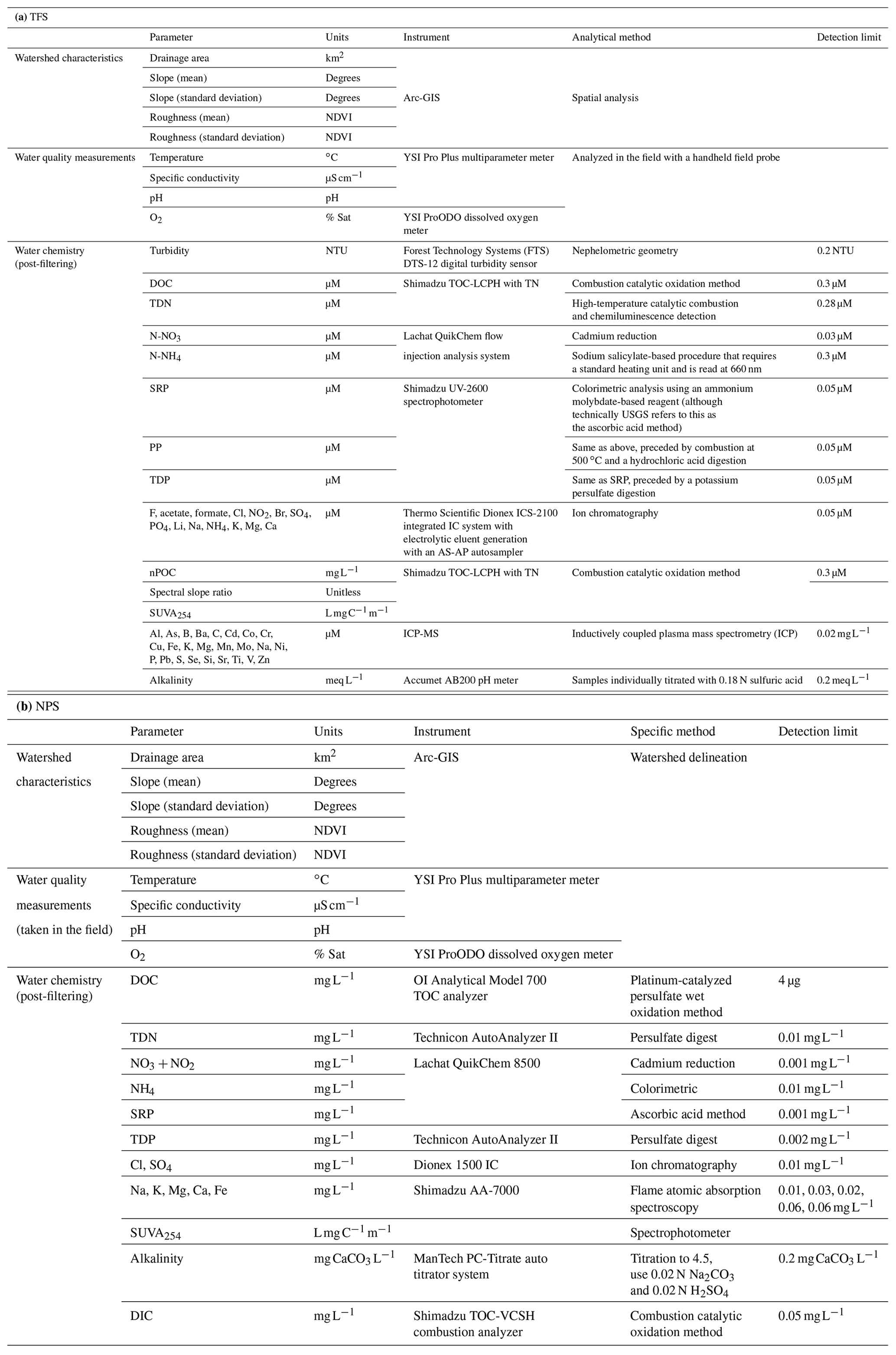
We include further detail on analytical methods and instrumentation in Table 3, though we briefly describe our methods here. We measured DOC (as non-purgeable organic carbon, nPOC) and total dissolved nitrogen (TDN) with a total carbon analyzer (Shimadzu TOC-LCPH with a total nitrogen analyzer and ASI-L autosampler). We determined dissolved organic matter (DOM) optical properties including the spectral ratio (S_r, unitless) and specific ultraviolet absorbance at 254 nm (SUVA₂₅₄) from the TOC and TN dataset (Helms et al., 2008; Hansen et al., 2016). We colorimetrically analyzed SRP, particulate phosphorous (PP), and total dissolved phosphorous (TDP) on a spectrophotometer (Shimadzu UV-2600). We quantified inorganic nitrogen species (nitrate, NO₃; ammonium, ${{\mathrm{NH}}_{\mathrm{4}}}^{+}$) using a flow-through injection analysis (Lachat QuikChem flow injection analysis system). We measured several cations (Na⁺, Li⁺, K⁺, Mg²⁺, Ca²⁺, ${{\mathrm{NH}}_{\mathrm{4}}}^{+}$), anions (F⁻, Cl⁻), oxoanions (${{\mathrm{NO}}_{\mathrm{2}}}^{-}$, ${{\mathrm{SO}}_{\mathrm{4}}}^{\mathrm{2}-}$, ${{\mathrm{NO}}_{\mathrm{3}}}^{-}$, ${{\mathrm{PO}}_{\mathrm{4}}}^{\mathrm{3}-}$), and organic acids (acetate, CH₃COO⁻; and formate, HCOO⁻) on an ion chromatography system (Thermo Fisher Scientific Dionex ICS5000). We quantified other geogenic anions and cations (e.g., Al³⁺, As³⁻, B³⁻, Ba²⁺, Br⁺, Ca²⁺, Cd²⁺, Co²⁺, ${{\mathrm{CrO}}_{\mathrm{4}}}^{-}$, nominally dissolved Cu and Fe, K⁺, ${{\mathrm{MoO}}_{\mathrm{3}}}^{\mathrm{2}-}$, Mg²⁺, Mn²⁺, Na⁺, Ni²⁺, P, Pb²⁺, S²⁻, Se²⁻, dissolved Si, Sn²⁺, Sr²⁺, Ti, V, Zn²⁺) on an inductively coupled plasma mass spectrometer (ICP-MS, iCAP 7000 series, Thermo Scientific). To estimate turbidity (NTU), we used benchtop UV–visible spectrophotometers (s::can Messtechnik GmbH, Vienna, Austria). We analyzed all samples at room temperature after allowing them to thaw on a lab bench for 2–4 h prior to analysis.

Table 3 Summary of sample processing and analytical methods used for the dataset for (a) TFS and (b) NPS/USGS field sites.

NPS/USGS

We include further detail on analytical methods and instrumentation in Table 3. For the NPS/USGS sites, we measured DOC and DIC (OI Analytical Model 700 TOC analyzer and Shimadzu TOC-VCSH combustion analyzer, respectively). We characterized DOM aromaticity by measuring UV–visible absorbance on filtered stream water samples on an Agilent model 8453 photodiode array and then calculating SUVA₂₅₄ (Weishaar et al., 2003). We also measured TDN and TDP on a Technicon AutoAnalyzer II. We quantified inorganic nitrogen species (${{\mathrm{NO}}_{\mathrm{3}}}^{-}+{{\mathrm{NO}}_{\mathrm{2}}}^{-}$ and unionized NH₃) and orthophosphate (${{\mathrm{PO}}_{\mathrm{4}}}^{\mathrm{3}-}$) using a flow-through injection analysis system (Lachat QuikChem 8500). We calculated alkalinity using a titration to a pH of 4.5, using 0.02 N Na₂CO₃ and 0.02 N H₂SO₄ (ManTech PC-Titrate auto titrator system). Finally, we used ion chromatography to measure Cl⁻ and ${{\mathrm{SO}}_{\mathrm{4}}}^{\mathrm{2}-}$ (Dionex 1500 IC) and absorption spectroscopy to measure Na⁺, K⁺, Mg²⁺, Ca²⁺, and total Fe (Shimadzu AA-7000).

3.3 Estimation of ecohydrological metrics

In addition to reporting solute concentrations for each synoptic campaign (e.g., Figs. 4 and 5), we estimated ecohydrological metrics for each nested site and watershed. Across these analyses, we assigned any value below detection as the values of half the limit of quantification and kept these data points in the analysis. When the sample was not run for a specific solute, the cell was left blank.

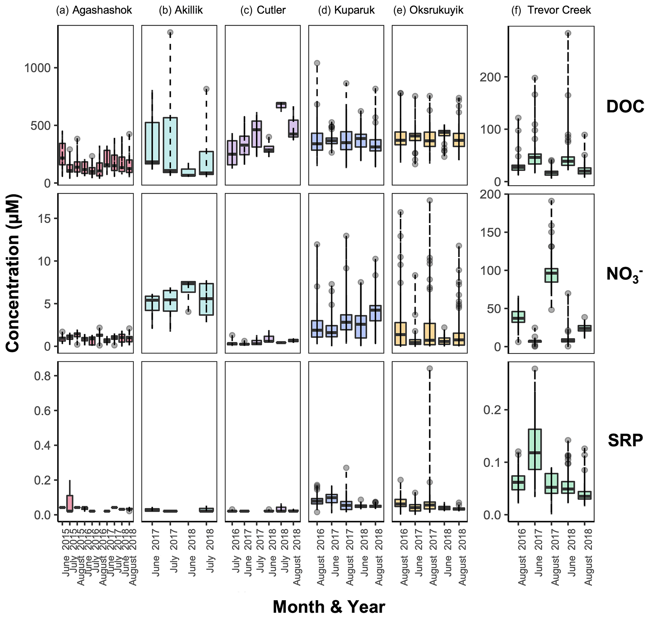
Figure 4 Boxplots of dissolved organic carbon (DOC, top row), nitrate (${{\mathrm{NO}}_{\mathrm{3}}}^{-}$, middle row), and soluble reactive phosphorus (SRP, bottom row) concentration ranges (in µM) in the (a) Agashashok River, (b) Akillik River, (c) Cutler River, (d) Kuparuk, (e) Oksrukuyik Creek, and (f) Trevor Creek watersheds across all years and seasons sampled. Each box encapsulates values within the lower 25th and upper 75th quartiles respectively, while the whiskers represent the minimum and maximum quartiles. Within each box, the horizontal line represents the median leverage value. Data points outside the whiskers represent values above and below 1.5× the interquartile range (IQR) threshold.

Figure 5 Boxplots of Ca²⁺, Cl⁻, Fe (total for NPS/USGS; nominally dissolved for TFS), K⁺, Mg²⁺, and total Si concentration ranges (in µM) in the (a) Agashashok River, (b) Akillik River, (c) Cutler River, (d) Kuparuk River, (e) Oksrukuyik Creek, and (f) Trevor Creek watersheds across all years and seasons sampled. Each box encapsulates values within the lower 25th and upper 75th quartiles respectively, while the whiskers represent the minimum and maximum quartiles. Within each box, the horizontal line represents the median leverage value. Data points outside the whiskers represent values above and below 1.5× the IQR threshold.

3.3.1 Subcatchment leverage

First, we estimated subcatchment leverage from each of the synoptic sampling events for each solute. Subcatchment leverage is calculated as the difference in terms of concentration at each site (C_s) from the concentration at the watershed outlet (C_o), subcatchment area (A_s) relative to the entire watershed area (A_o), and specific discharge at the sampling location ($q=Q_{\mathrm{s}}/A_{\mathrm{s}},$ where Q_s and A_s are the discharge and subcatchment area at the sampling point):

$$\begin{array}{}\text{(1)}& \mathrm{\text{specific subcatchment leverage}}=\left[(C_{\mathrm{s}}-C_{\mathrm{o}})\cdot {\displaystyle \frac{A_{\mathrm{s}}}{A_{\mathrm{o}}}}\cdot q\right].\end{array}$$

In the case of Eq. (1), leverage is expressed in units of flux (mass/volume/time). However, if specific discharge is unavailable for each sampling location, leverage can be estimated using only variability in concentration and subcatchment area, so long as specific discharge (q) is similar between subcatchments (Asano et al., 2009; Karlsen et al., 2016). With the exception of the Agashashok River, which has flow generated from deeper flow paths, our study watersheds have very little regional groundwater influence (Lecher, 2017), and the synoptic campaigns were performed near base-flow conditions. Therefore, for the purposes of this study, we assumed that q was similar for subcatchments within a study watershed but not necessarily across the six study watersheds. This assumption was tested at all Arctic LTER sites using dilution gauging at a subset of sites in summer 2018 and 2019, where we found that values of specific discharge were similar across subcatchment sizes (Arial J. Shogren, unpublished data). We used Eq. (2) to estimate subcatchment leverage for all sampling locations across sampling events:

$$\begin{array}{}\text{(2)}& \text{subcatchment leverage (\%)}=\mathrm{100}\cdot \left[(C_{\mathrm{s}}-C_{\mathrm{o}})\cdot {\displaystyle \frac{A_{\mathrm{s}}}{A_{\mathrm{o}}}}\right].\end{array}$$

Here, subcatchment leverage has units of concentration, or percentage when normalized to outlet concentration. In other words, the distributed mass balance is relative to a pre-determined outflow point; with the presented analysis, we used the furthest downstream point with the largest drainage area as our outlet location. The interpretation of leverage values is opposite at the site and watershed scales (Abbott et al., 2018; Shogren et al., 2019). For example, a site with a positive value for subcatchment leverage is contributing more than the typical subcatchment in the watershed. Conversely, a watershed with a mean leverage value that is positive is indicative of a net removal in the stream network because there is more solute in the tributaries than can be accounted for at the watershed outlet, while a negative value suggests solute production in the network (Abbott et al., 2018; Shogren et al., 2019). We report both mean leverages for each catchment (presented in Figs. 6 and 7) and site-specific subcatchment leverages for each solute (Fig. 10 for DOC and ${{\mathrm{NO}}_{\mathrm{3}}}^{-}$, but all other solutes can be found within the ecohydrological metrics datasets).

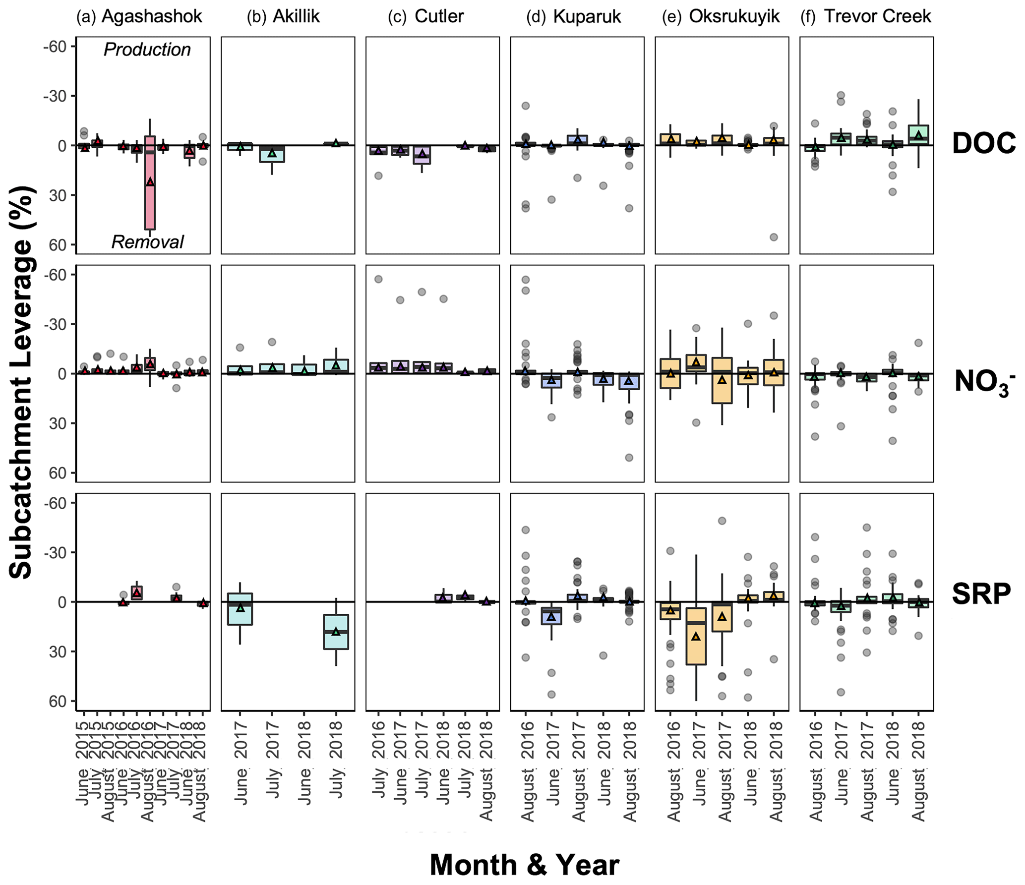
Figure 6 Boxplot of subcatchment leverage for select reactive solutes (DOC, ${{\mathrm{NO}}_{\mathrm{3}}}^{-}$, and SRP) in the (a) Agashashok River, (b) Akillik River, (c) Cutler River, (d) Kuparuk River, (e) Oksrukuyik Creek, and (f) Trevor Creek watersheds across all years and seasons sampled. Note reversed axes for ease of interpretation: negative values above the 0 line indicate production; positive values below the 0 line indicate removal. Each box encapsulates values within the lower 25th and upper 75th quartiles respectively, while the whiskers represent the minimum and maximum quartiles. Within each box, the horizontal line represents the median leverage value and the colored triangle lies at the mean. Data points outside the whiskers represent values above and below 1.5× the IQR threshold.

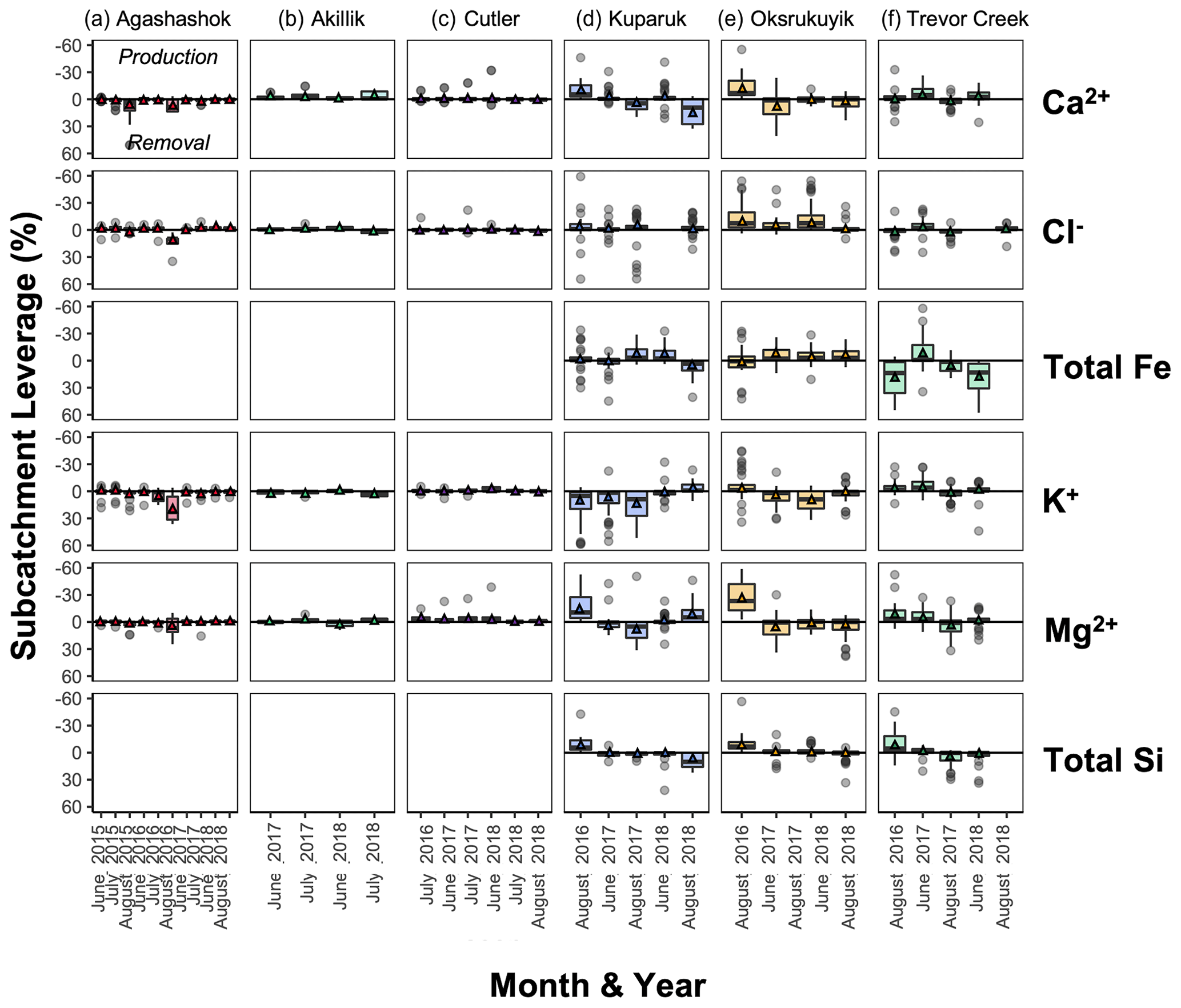
Figure 7 Boxplot of subcatchment leverage for select conservative solutes (Ca²⁺, Cl⁻, Fe (total for NPS/USGS; nominally dissolved for TFS), K⁺, Mg²⁺, and total Si) in the (a) Agashashok River, (b) Akillik River, (c) Cutler River, (d) Kuparuk River, (e) Oksrukuyik Creek, and (f) Trevor Creek watersheds across all years and seasons sampled. Note reversed axes for ease of interpretation: negative values above the 0 line indicate production; positive values below the 0 line indicate removal. Each box encapsulates values within the lower 25th and upper 75th quartiles respectively, while the whiskers represent the minimum and maximum quartiles. Within each box, the horizontal line represents the median leverage value and the colored triangle lies at the mean. Data points outside the whiskers represent values above and below 1.5× the IQR threshold.

3.3.2 Concentration variance collapse

Next, to assess the representative patch size where concentration variance is reduced, we determined the threshold of concentration variance collapse for each solute from each synoptic sampling event (shown in Fig. 8). Using concentrations plotted over watershed area, we used the changepoint package in R (Killick and Eckley, 2014) to determine the collapse in variance of concentration across the whole watershed area. To determine the reduction in variance statistically, we used the pruned exact linear time (PELT) method, which compares differences in data points to determine statistical breakpoints (Abbott et al., 2018; Shogren et al., 2019). We performed this analysis using scaled concentrations, which were scaled by subtracting the whole watershed mean and dividing by the standard deviation to facilitate comparison of changes in variance and evaluate convergence towards the watershed mean. The variance collapse threshold is therefore expressed in units of area (here as km²). A non-significant variance collapse threshold can be interpreted to mean either the processes controlling lateral fluxes are operating at too small or too large a scale to be captured using a subcatchment sampling approach.

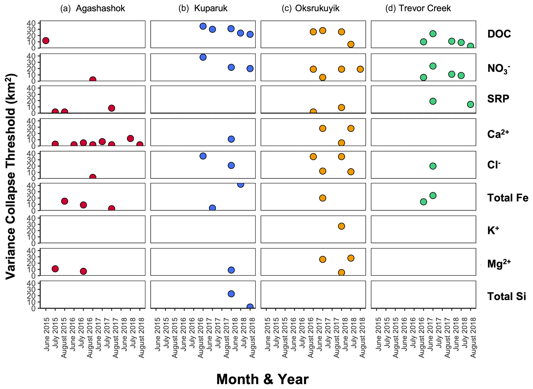
Figure 8 Scatter plot of variance collapse threshold for each repeated sampling for the (a) Agashashok River, (b) Kuparuk River, (c) Oksrukuyik Creek, and (d) Trevor Creek watersheds for select reactive (e.g., DOC, ${{\mathrm{NO}}_{\mathrm{3}}}^{-}$, and SRP) and conservative solutes (Ca²⁺, Cl⁻, Fe (total for NPS/USGS; nominally dissolved for TFS), K⁺, Mg²⁺, and total Si). When data were not present, there was no significant collapse detected. Variance collapse thresholds are not shown for the Akillik and Cutler rivers, as these thresholds were often non-significant.

3.3.3 Spatial persistence

Lastly, we analyzed this spatially rich synoptic data to quantify the spatial persistence of stream nutrient concentrations and to determine the level of sub-grid resolution necessary to represent controls on lateral nutrient loss. The spatial persistence metric indicates whether spatial sampling is representative or whether spatial patterns reshuffle over time. Spatial persistence (r_s) is calculated as

$$\begin{array}{}\text{(3)}& \left(r_{\mathrm{s}}\right)=\left({\displaystyle \frac{\text{covariance}({\text{rg}}_x,{\text{rg}}_y)}{{\mathit{\sigma }}_{{\text{rg}}_x}{\mathit{\sigma }}_{{\text{rg}}_y}}}\right),\end{array}$$

where rg_x is the rank of subcatchments at the time of synoptic sampling, rg_y is the rank of the long-term flow-weighted concentrations, while ${\mathit{\sigma }}_{{\text{rg}}_x}$ and ${\mathit{\sigma }}_{{\text{rg}}_y}$ are the standard deviation of the rank variables. We calculated spatial persistence using the correlation function in R (version 3.3.0), using the Spearman method (Abbott et al., 2018; Shogren et al., 2019). Significance was tested using a Student t distribution test. Additional methods for calculating spatial persistence have now been proposed that do not require discharge data for the flow weighting (Gu et al., 2021). For the purposes of the Arctic LTER analysis, we estimated spatial persistence as the Spearman's correlation between early (June) and late (August) site concentrations, resulting in a single spatial persistence metric (r_s) for 2017 and 2018. For the NPS/USGS sites, spatial persistence was calculated as the correlation between site locations sampled in the early (June) and mid (July) and the mid to late (August or September) seasons.

3.4 Use and interpretation of ecohydrological ecosystem metrics

The original intent of this paper was to present our unique Arctic datasets and showcase the utility of a synoptic framework in combination with metrics that describe the spatial distribution of river chemistry. To further highlight how these metrics can inform future sampling design and address fundamental ecological questions, below we describe patterns for DOC and ${{\mathrm{NO}}_{\mathrm{3}}}^{-}$ in the TFS watersheds.

For solutes, the spatial variability in concentration depends on the strength and connectivity of both source and sink patches superimposed on the structure of the stream network (Abbott et al., 2018). When we plot solute concentration against subcatchment area, we find more variability water chemistry in smaller subcatchments (<30 km²). This can be interpreted as a spatial fingerprint and is shown most clearly in Fig. 10, which displays the spatial distribution of DOC and ${{\mathrm{NO}}_{\mathrm{3}}}^{-}$ concentrations across watersheds and sampling campaigns. Generally high concentration variability in smaller headwaters, which converges to mean watershed behavior towards the catchment outlet, holds with the conceptualizations of large rivers as chemostats (Creed et al., 2015). In the context of Arctic watersheds, these concentration–area relationships reveal consistently high DOC and low ${{\mathrm{NO}}_{\mathrm{3}}}^{-}$ concentrations in the low-gradient tundra watersheds (Kuparuk River and Oksrukuyik Creek), despite high variability in smaller contributing subcatchments. In contrast, the alpine watershed Trevor Creek has relatively low DOC and high ${{\mathrm{NO}}_{\mathrm{3}}}^{-}$ concentrations, likely due to shorter and faster hydrologic flow paths and lower terrestrial biomass (Shogren et al., 2019). Overall, these findings are consistent with studies that indicate that slower, longer flow paths and productive terrestrial vegetation control carbon and nutrient transfer and mobilization in lower-gradient tundra watersheds (Shogren et al., 2019, 2021). If we assume that spatial variability in stream network water chemistry depends primarily on the extent and connectivity of upstream sources and sinks, then the patch sizes that control solute fluxes can be assessed by the spatial scale of the variance collapse (Abbott et al., 2018; Shogren et al., 2019). Across all three TFS watersheds, the generality of variance collapse at intermediate scales is indicative that subcatchment-scale patches (∼10–50 km²) control whether carbon and inorganic nitrogen is produced or removed at the watershed scale (Fig. 10). In addition, the consistency of the thresholds across sampling campaigns (Figs. 8 and 10) highlights the importance of capturing intermediate-scale biogeochemistry to bridge understandings from plot-level experimentation to larger more regional-scale observations (Shogren et al., 2019).

Figure 9 Scatter plot of spatial stability (r_s) for each repeated sampling for the (a) Agashashok, (b) Kuparuk River, (c) Oksrukuyik Creek, and (d) Trevor Creek watersheds for select reactive (e.g., DOC, ${{\mathrm{NO}}_{\mathrm{3}}}^{-}$, and SRP) and conservative solutes (Ca²⁺, Cl⁻, Fe (total for NPS/USGS; nominally dissolved for TFS), K⁺, Mg²⁺, and total Si). When data were not present, there is no spatial stability reported. When Spearman's rank correlation (r_s) is significant, this is denoted by an asterisk (∗) within the point.

Figure 10 Scatter plot of log-scale (a) DOC and (b) ${{\mathrm{NO}}_{\mathrm{3}}}^{-}$ concentrations (µM) across subcatchment area (km²) or each repeated sampling in the Kuparuk River (blue points), Oksrukuyik Creek (orange points), and Trevor Creek (green points) watersheds. Significant variance collapse thresholds are represented by a colored arrow.

When we convert concentrations into estimates of subcatchment leverage (e.g., Figs. 6, 7, 10, and 11), patterns emerge that further contextualize the spatial distribution of DOC and ${{\mathrm{NO}}_{\mathrm{3}}}^{-}$ concentrations. First, we can investigate whole watershed (net) behavior by calculating the mean leverage and examining the distribution of values with boxplots (as in Figs. 6 and 7). As a more specific example, mean ${{\mathrm{NO}}_{\mathrm{3}}}^{-}$ leverage within the Kuparuk watershed (Fig. 6d, second row) were consistently above zero (note the reversed axis), revealing strong removal or retention before it reached the watershed outlet, which is consistent with high biotic N demand. Within this same watershed, DOC leverage values were often at or just above the zero line (Fig. 6d, first row), representing primarily conservative transport of DOC (i.e., no net production or uptake). Within the lake-influenced Oksrukuyik watershed, ${{\mathrm{NO}}_{\mathrm{3}}}^{-}$ leverage values were more variable (i.e., leverage above and below the zero line; Fig. 6e, second row), implying a combination of removal and production mechanisms acting across the watershed network. When visualized as net behavior, the watershed and season-dependent directionality of net leverage patterns are congruent with emerging evidence that landscape template exerts strong control on biogeochemical signals in Arctic rivers (Vonk et al., 2019; Tank et al., 2020; Shogren et al., 2021). As a complement to the first approach, we can additionally examine individual subcatchment leverage values to reveal the effect of each contribution on what we observe at the watershed outlet. This can be interpreted similarly to statistical leverage, where one or more points may exert high influence on a linear regression.

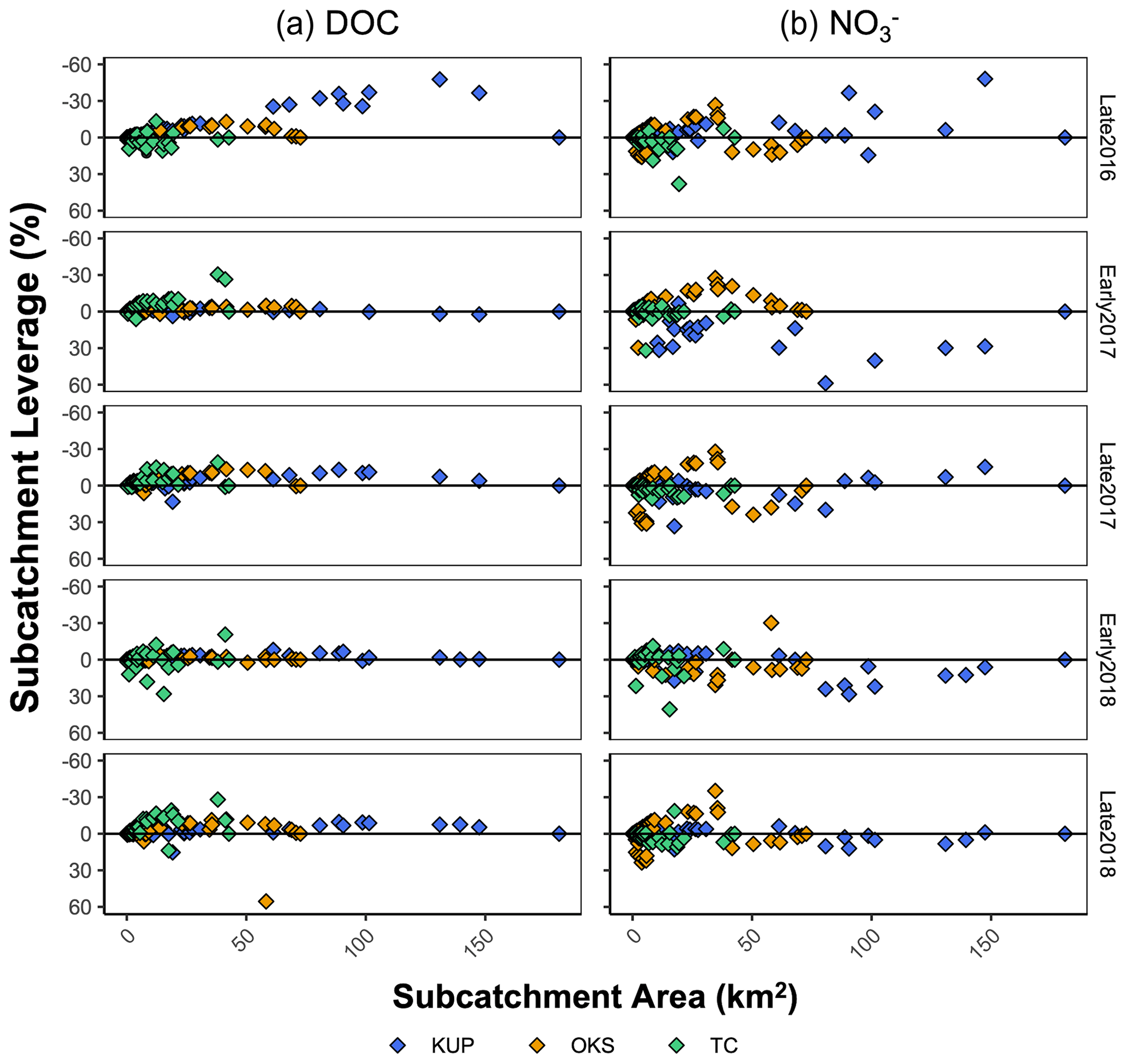
Figure 11 Scatter plot of (a) DOC and (b) ${{\mathrm{NO}}_{\mathrm{3}}}^{-}$ leverages across subcatchment area (km²) or each repeated sampling in the Kuparuk River (blue points), Oksrukuyik Creek (orange points), and Trevor Creek (green points) watersheds. Note reversed axes for ease of interpretation: negative values above the 0 line indicate production; positive values below the 0 line indicate removal.

Across all TFS watersheds, there are a few select subcatchments that contribute disproportionately to DOC fluxes, while the more variable patterns for ${{\mathrm{NO}}_{\mathrm{3}}}^{-}$ suggest additional spatial and seasonal controls (Fig. 11). For example, patterns in the Kuparuk River and Oksrukuyik Creek (Fig. 11a and b) could be interpreted to mean that DOC is transported conservatively in lower-gradient landscapes, while lateral fluxes of ${{\mathrm{NO}}_{\mathrm{3}}}^{-}$ are more tightly controlled by biotic demand (Harms et al., 2016; Khosh et al., 2017; Connolly et al., 2018; Kendrick et al., 2018; Iannucci et al., 2021). Across solutes and watersheds, the information gleaned from the leverage metric is useful in several ways. First, subcatchment leverages allow for the direct identification of watershed areas that are disproportionately driving carbon and nutrient exports. For any chosen solute or suite of materials, sites identified as “high leverage” indicate strong source/sink behavior, which could be (1) validated with regular field observations that relate riparian or terrestrial conditions with empirical measurements of water chemistry, (2) selected for further study designed to identify the abiotic and biotic mechanisms that drive patterns of riverine chemistry, and/or (3) identified as non-representative sites relative to proximal subcatchments of similar size and terrestrial characteristics. Relatedly, estimating subcatchment leverage enables researchers to identify sites that are representative of watershed-scale behavior, which could be used to more effectively scale biogeochemical dynamics in Arctic rivers relative to outlying subcatchments (Kicklighter et al., 2013; Pinay et al., 2015; Aguilera et al., 2013).

Finally, the application of the simple spatial persistence metric can help researchers determine whether a sampling location is behaving consistently, or if solute contributions are moving in space across sampling events (Abbott et al., 2018; Dupas et al., 2019). In the context of work in remote watersheds, the ability for researchers to identify both stable and unstable processes presents an exciting opportunity to ask questions about the consistency of subcatchment contributions and optimize sampling or experimental design. For example, DOC concentrations are generally spatially stable between early and late sampling events (r_s>0.50), particularly in the Kuparuk River and Trevor Creek watersheds (Fig. 9). In these landscapes, a high rank correlation indicates that repeated sampling of the same location will result in a similar spatial distribution of concentrations. While sampling repeatedly in the early and late seasons may reveal increases or decreases in solute concentrations (Shogren et al., 2019), the high degree of relatedness indicates that these patterns will be maintained across the watershed network. However, the low persistence (r_s<0.50) for DOC in the Oksrukuyik Creek watersheds signifies substantial spatial shifts across the early and late thaw season (Shogren et al., 2019). While there was variability in the persistence across watersheds and solutes, the stability metric can be used by future researchers to identify whether sampling the same location repeatedly does or does not represent the spatial dynamics across sampling events.

4 Data availability

The data from the NPS/USGS are available at https://doi.org/10.5066/P9SBK2DZ (O'Donnell et al., 2021). Data from TFS are stored at the Environmental Data Center data repository (https://doi.org/10.6073/pasta/258a44fb9055163dd4dd4371b9dce945, Abbott, 2021).

5 Conclusions

With this work, we provide a detailed characterization of physical, chemical, and biological parameters that are essential to using river network chemistry to infer ecosystem-level carbon and nutrient balance. We apply novel metrics to these data that describe the spatiotemporal patterns of watershed biogeochemistry in six permafrost-underlain Arctic watersheds. These data represent a high-resolution and temporally replicated river chemistry dataset from understudied permafrost-dominated regions. Combining these measures with remotely sensed data, plot-level experiments, and numerical models could advance our understanding of permafrost ecosystems in the face of climate change and other disturbance.