the Creative Commons Attribution 4.0 License.
the Creative Commons Attribution 4.0 License.
 | 21 Feb 2022
A new Greenland digital elevation model derived from ICESat-2 during 2018–2019
Yubin Fan
Chang-Qing Ke
Xiaoyi Shen
Greenland digital elevation models (DEMs) are indispensable to fieldwork, ice velocity calculations, and mass change estimations. Previous DEMs have provided reasonable estimations for all of Greenland, but the time span of applied source data may lead to mass change estimation bias. To provide a DEM with a specific time stamp, we applied approximately 5.8×10⁸ ICESat-2 observations from November 2018 to November 2019 to generate a new DEM, including the ice sheet and glaciers in peripheral Greenland. A spatiotemporal model fit process was performed at 500 m, 1 km, 2 km, and 5 km grid cells separately, and the final DEM was posted at the modal resolution of 500 m. A total of 98 % of the grids were obtained by the model fit, and the remaining DEM gaps were estimated via the ordinary Kriging interpolation method. Compared with IceBridge mission data acquired by the Airborne Topographic Mapper (ATM) lidar system, the ICESat-2 DEM was estimated to have a maximum median difference of −0.48 m. The performance of the grids obtained by model fit and interpolation was similar, both of which agreed well with the IceBridge data. DEM uncertainty rises in regions of low latitude and high slope or roughness. Furthermore, the ICESat-2 DEM showed significant accuracy improvements compared with other altimeter-derived DEMs, and the accuracy was comparable to those derived from stereophotogrammetry and interferometry. Overall, the ICESat-2 DEM showed excellent accuracy stability under various topographic conditions, which can provide a specific time-stamped DEM with high accuracy that will be useful to study Greenland elevation and mass balance changes. The Greenland DEM and its uncertainty are available at https://doi.org/10.11888/Geogra.tpdc.271336 (Fan et al., 2021).
- Article
(15158 KB) - Full-text XML
- BibTeX
- EndNote


Greenland's digital elevation model (DEM) is particularly important for fieldwork planning and numerical modeling verification (Bamber et al., 2009). The ice deformation rate and the underlying bedrock condition can be measured with ice thickness data, which is useful to determine subglacial hydrological pathways (Bamber et al., 2013). The surface elevation at different periods is also indispensable for studying elevation and mass changes to understand ice dynamics and estimate potential sea level changes (Sutterley et al., 2014; Smith et al., 2020). In addition, InSAR (interferometric synthetic aperture radar) estimation of ice velocity requires high-accuracy and up-to-date DEMs to distinguish phase differences caused by terrain and ice sheet movement (Riel et al., 2021).
The first published Greenland DEM dates back to the 1980s, providing elevations of peripheral Greenland generated through 3500 photographs from 1978 to 1987 with a resolution of 25 m (Korsgaard et al., 2016). However, the low-visibility contrast between snow and ice surfaces may affect the radiometric and geometric quality of stereoscopic DEMs (Noh and Howat, 2015), which may introduce considerable uncertainty to the elevation. Research regions were also restricted to the margin and outlets of Greenland, and there is a lack of understanding about the internal ice sheet.
The currently available DEMs of all of Greenland include those based on stereophotogrammetry, altimeters, and interferometry. Most DEMs were derived from stereophotogrammetry images, such as the Greenland Ice Mapping Project (GIMP) DEM (version 1) derived from ASTER (Advanced Spaceborne Thermal Emission and Reflection Radiometer), SPOT 5 (Satellite pour l'Observation de la Terre), and AVHRR (Advanced Very High Resolution Radiometer) photoclinometry (Howat et al., 2014), as well as GIMP2 and ArcticDEM derived from GeoEye-1, WorldView-1, WorldView-2, and WorldView-3. ArcticDEM was the latest released DEM, with the highest resolution (2 m) among all free available Greenland DEMs. Optical image pairs may be influenced by weather, clouds, and the solar elevation angle (Korona et al., 2009); thus, the posted DEM is the combination of images of long time spans, which might limit its scientific applications to mass balance research. In addition, owing to the wide coverage (86∘ N–86∘ S), high single-point accuracy (0.1–0.15 m), and small footprint size (70 m) (Zwally et al., 2002), ICESat has the ability to measure the elevation of all of Greenland. Hence, a bi-quadratic surface to fit ICESat footprints within each 1 km grid was adopted to obtain the ICESat DEM, but the largest search radius of 20 km in the low-latitude regions to some extent limited the ability to describe the small-scale elevation patterns at the Greenland margin (DiMarzio et al., 2007). A Ku-band synthetic aperture interferometric radar altimeter (SIRAL) carried by CryoSat-2 further increases the spatial coverage within 88∘ N–88∘ S. Although the footprint size (approximately 300 m) was larger than that of ICESat, the smaller cross-track distance (2.5 km) still ensures its ability to monitor the ice sheet (Wingham, 2002); thus, CryoSat-2 L1B data from 2011 to 2014 were applied to generate the Cryosat-2 DEM through the Kriging interpolation approach (Helm et al., 2014). Coarse across-track resolution is the major limitation to applying laser altimeters to generate a DEM with finer resolution (<1 km) in Greenland. TanDEM-X and TerraSAR-X were also used to generate the Greenland DEM using differential interferometry (Zink et al., 2014), but the X-band radar signal penetration depth into the dry snowpack may cause the elevation to be underestimated by several meters (Dehecq et al., 2016). These DEMs provide reasonable estimations for all of Greenland, but the specific timestamps of the current DEMs were missing.
ICESat-2, with a new generation satellite-borne lidar altimeter, is intended as a successor to the ICESat mission to quantify the contribution of polar ice sheets to sea level rise and the impact of climate change (Markus et al., 2017). ICESat-2 has an orbital altitude of 500 km and an orbital inclination of 92∘, including a revisit period of 91 d, and can provide centimeter-scale measurements of different surface types. The ICESat-2 beam footprint of approximately 17 m with a spatial interval of 0.7 m ensures accurate elevation measurements at a high orbital resolution by determining the local ice sheet slope (Neumann et al., 2019). A much finer observation can be obtained owing to its along-track distance of 0.7 m and cross-track distance of 3.3 km, which is a significant improvement compared with CryoSat-2's along-track distance of 0.3 km and cross-track distance of 1.5 km, as well as ICESat's along-track distance of 170 m. Not only the resolution but also the accuracy has been improved. The accuracy in the flat ice sheet can reach 3 cm, and it can still be less than 14 cm even for complex topography (Shen et al., 2021), which makes ICESat-2 a great data source to generate a DEM with high resolution and accuracy.
Here, we present a novel Greenland DEM (ICESat-2 DEM) in May 2019 with a 500 m resolution using a spatiotemporal model fit based on ICESat-2 measurements from November 2018 to November 2019. The overall accuracy of ICESat-2 DEM was evaluated by comparing it to the spatiotemporally matched IceBridge data. The performance was also compared with other published DEMs under various terrain conditions to validate the reliability of the ICESat-2 DEM.
2.1 ICESat-2 ATL06 data
The ICESat-2 land ice height product ATL06 (release 003) was used here for DEM generation. The product provides longitude, latitude, and surface heights based on the WGS84 ellipsoid. The ATL06 product is developed from global geolocated photon data (ATL03) to estimate the land ice height (Smith et al., 2019). Compared with the original ATL03 product, land ice height is determined after instrument bias corrections (e.g., transmit pulse shape bias correction and first-photon bias correction) (Markus et al., 2017). The beam pair separation of the ATL06 product is set at 3.3 km across the track. The three pairs contain one strong beam and one weak beam, and the two beams within each pair are separated by 90 m distance.
Brunt et al. (2019) compared the elevation of the ICESat-2 ATL06 product and GPS data and found that the accuracy differences of strong and weak beams are less than 2 cm. Shen et al. (2021) compared ICESat-2 ATL06 product with IceBridge data under complex terrain, and the results indicated that the height difference between them is also trivial. Hence, we included weak beams to increase spatial coverage and data point utilization because no systematic errors were found in strong and weak beams in ICESat-2 elevation measurements. However, only data marked as good quality (atl06_quality_summary = 0) were used for DEM generation to improve the accuracy of the DEM. Over all of Greenland ice sheet and outlet glaciers, we used approximately 5.8×10⁸ ICESat-2 elevation footprints to generate a new DEM, that is, the ICESat-2 DEM.
2.2 IceBridge data
To evaluate the accuracy of the ICESat-2 DEM, we used Airborne Topographic Mapper (ATM) surface elevation data from the IceBridge survey. The ATM was intended to fill the gap between ICESat and ICESat-2, working at the same wavelength (532 nm) as ICESat-2. The absolute elevation accuracy of the ATM system can reach 0.1 m, and the position accuracy on the flat ice sheet is less than 1 m (Kurtz et al., 2013). The IceBridge ATM L2 Icessn Elevation, Slope, and Roughness Version 2 dataset was used to evaluate the DEMs. The final resolution of IceBridge was resampled to 25 m, and the estimated error was approximately 12 cm (Krabill et al., 2004). The root-mean-square error (RMSE) was taken as the roughness of each IceBridge data point. The slope and aspect of IceBridge were described in Shen et al. (2021).

Figure 1IceBridge data acquired in May 2019 which were used to evaluate the generated ICESat-2 DEM, covering regions in Greenland with various terrain conditions: (a) elevation, (b) slope, (c) aspect, and (d) roughness. Labels in the picture are the main glaciers in Greenland.
During 2009–2019, IceBridge provided millions of footprints over Greenland, covering both the peripheral and inland areas of Greenland. The distribution of IceBridge data for May 2019, which was used to evaluate the accuracy of the new ICESat-2 DEM, is displayed in Fig. 1. We also calculated the histogram of the elevation, surface slope, surface aspect, and roughness of IceBridge in May 2019. Overall, the elevations of the sampled regions ranged from 0 to 3500 m, the surface slopes ranged from 0 to 10∘, the surface aspects ranged from 0 to 360∘, and the roughnesses ranged from 0 to 20 cm (Fig. 2). These sampled areas had variable surface terrain conditions, which provided a reliable dataset to evaluate the performance of the ICESat-2 DEM.
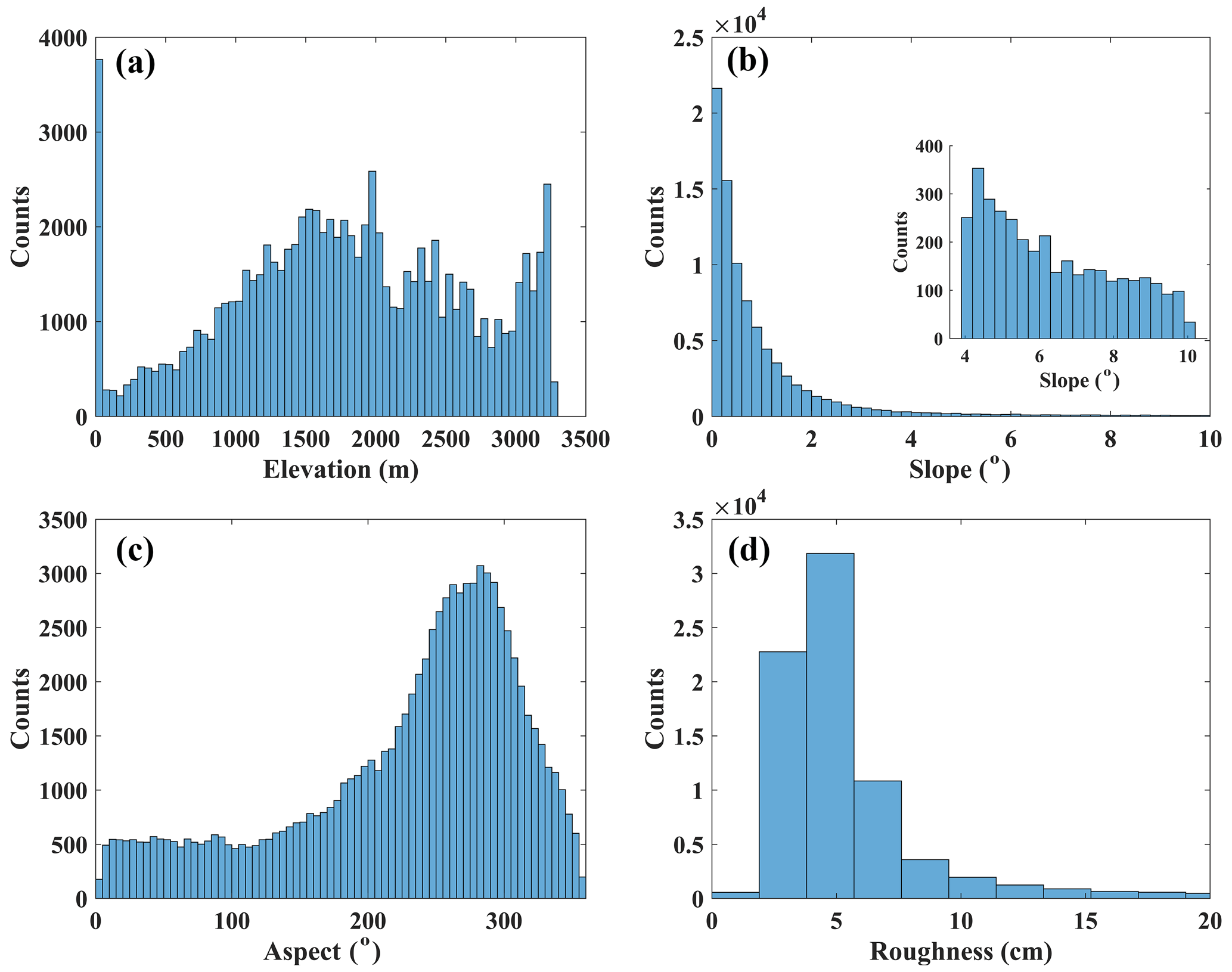
Figure 2Histogram of the (a) surface height, (b) surface slope, (c) aspect, and (d) roughness derived from IceBridge data. The inset figure shows the histogram of surface slope between 4 and 10∘.
2.3 Other available Greenland DEMs
We used other published DEMs to compare the performance of the generated ICESat-2 DEM; the detailed information concerning these DEMs is provided in Table 1, and all DEMs have been referenced to the WGS84 ellipsoid.
Table 1Published Greenland DEMs used in this study. Note that the ArcticDEM has higher resolutions of 2, 10, 32, and 100 m and that we used only resolutions of 500 and 1000 m for comparison.

2.3.1 GLAS/ICESat 1 km laser altimetry DEM
Greenland's DEM, derived from GLAS/ICESat (Geoscience Laser Altimeter System) laser altimetry data (from February 2003 to June 2005), provides the surface elevation for both Greenland ice sheets and caps, with less impact on slopes compared with radar altimetry data such as EnviSat and ERS-1 and ERS-2. The spatial resolution is 1 km. The horizontal coordinates are based on the polar stereographic coordinate system.
2.3.2 ArcticDEM
ArcticDEM is a high-resolution, high-quality digital surface model (DSM) of the Arctic at different spatial resolutions (2, 10, 32, 100, 500, and 1000 m), and its temporal coverage is from 2015 to 2018. The mosaicked DEM results are compiled from the best-quality strip DEMs, and the filtered ICESat altimetry data are applied to improve the absolute accuracy. The estimated accuracy is approximately 85 cm at a resolution of 100 m (Xing et al., 2020). We used the elevation products of 500 and 1000 m for comparisons.
2.3.3 TanDEM-X DEM
The TanDEM-X DEM (TanDEM) is a global DEM with a resolution of 90 m provided by the German Aerospace Center (DLR). Data collection was completed in 2015, and global DEM production was completed in 2016 and published in 2018. Different from previous datasets, it was generated by two X-band radar satellites (TanDEM-X and TerraSAR-X), which provide synchronous information to create a high-accuracy DEM around the Earth's land surface. The absolute horizontal and vertical accuracy is less than 10 m. The temporal coverage of the TanDEM data is mainly from 2011 to 2014.
2.3.4 CryoSat-2 DEM
CryoSat-2 L1B data from January 2011 to January 2014 were used to provide the elevation of Greenland. Here, Helm et al. (2014) used waveform re-tracking to process low-resolution mode (LRM) data and applied interferometry to process interferometric synthetic aperture radar (InSAR) data. Besides, they also leveraged slope correction to improve original product elevation accuracy. The bias of the CryoSat-2 DEM was less than 1 m in flat regions and less than 4 m in rugged regions, showing similar performance to the other DEMs obtained by laser and radar altimeters.
3.1 DEM generation
We followed the method of Slater et al. (2018) to compute the elevation of Greenland, which is an iterative least-squares fit model to all the elevation measurements in each grid as a quadratic surface. This model is described by Eq. (1).
where hi is elevations derived from ICESat-2 measurement points in one grid, h represents the modeled elevation, a0, a1, a2, a3, and a4 are surface elevation fluctuations, is the elevation change rate in the 13 months, t is the month difference between May 2019 and the ICESat-2 acquisition time, tmid is the time of the mid timestamp (May 2019), and (x,y) are the coordinates in the polar stereographic projection.
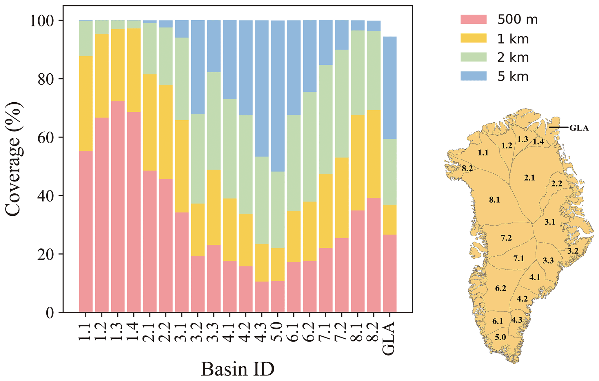
Figure 3Coverage percentages of calculated elevation grids by ICESat-2 observations of 500 m, 1 km, 2 km, and 5 km. The basin boundaries are from Zwally et al. (2002), which divides Greenland into eight main basins, covering approximately 1.72×10⁶ km2. Ice caps and glaciers that are not connected with the ice sheet are marked as GLA (glacier).
We found that there were more voids in low-altitude areas due to the low density of ICESat-2 footprints during the procedure of Greenland DEM generation. Therefore, it is necessary to select a suitable spatial resolution to produce the DEM with fewer gaps. DEM accumulated within 250 m grids only covered 15.38 % of the Greenland area and 30 % even at high latitudes; hence, we discarded this resolution from further processing. In contrast, a 500 m resolution increases overall coverage to 33 % and nearly 70 % at high latitudes (Fig. 3). With a 1 and 2 km resolution, the proportion of calculated portions exceeds 90 % in the regions that are north of 75∘ N (basins 1, 2, and 8). However, a 2 km resolution cannot obtain optimal coverage in low-elevation areas, while a 5 km resolution can further increase the coverage in the southern basins (basins 4, 5, and 6).
To reduce the effect of any poor fit, quality control was constrained in terms of data availability, quality, and rationality. We set the minimum number of grid points to 10 and the minimum timestamp to 2 months, which could ensure that enough measurements were contained in a grid cell to generate a reliable DEM. We assumed that the maximum elevation change is 10 m yr−1 and that its uncertainty cannot exceed 0.4 m yr−1 (Slater et al., 2018). Furthermore, we assumed that DEM uncertainty is less than 10 m and the maximum RMSE in each grid is 10 m. After this filter procedure, the elevation range is −500–3600 m, and this result is feasible since it is within the elevation range of published Greenland DEM products.
After the aforementioned process, we have acquired the Greenland DEM at four resolutions (500 m, 1 km, 2 km, and 5 km). However, these four types of DEM all include void areas; thus, we need to incorporate them to obtain the final Greenland DEM results with minimal gaps. First, we used the Greenland DEM with 500 m resolution as our first DEM source. Afterwards, Greenland DEMs with 1, 2, and 5 km resolutions were resampled to 500 m by applying a bilinear method to fill the gaps in this DEM and the finer resolution as our first option. Unavoidably, there are still some voids in the final Greenland DEM, but this has a minor impact on DEM accuracy. In this study, we described the unvoided area (98 %) in the final Greenland DEM as “calculated grids” and termed the rest (2 %) as “interpolated grids”. For the rest, an ordinary kriging approach was used for interpolation. The ICESat-2 DEM was posted at a modal resolution of 500 m after gap filling and interpolation. A median filter of 2.5 km×2.5 km was applied to the posted ICESat-2 DEM to minimize the influence of different resolutions.
Here, we applied different methods to estimate ICESat-2 DEM uncertainties in calculated grids and interpolated grids. The elevation uncertainty of the calculated grids was calculated by Eq. (2) based on MATLAB R2018a. For interpolated grid uncertainty estimation, we just used the kriging variance error calculated by ArcGIS 10.6. There is a 95.5 % probability that the actual elevation at the grid is the predicted raster value ± 2 times the square root of the variance error of the corresponding cell by assuming the kriging errors are normally distributed. Hence, 2 times the square root of the value in the variance error was taken as the elevation uncertainty in the interpolated grids (Eq. 3).
where bi is the elevation, SE (bi) is the standard error of the elevation, t (1–0.025, n−p) is the 95 % percentile of t distribution with n−p degrees of freedom, n is the number of ICESat-2 measurements in one grid, p is the number of regression coefficients (i.e., seven), and variance error is kriging variance error.
The slope was calculated by the method of Horn (1981); thus, the slope uncertainty was calculated based on the law of propagation:
where σei is the elevation uncertainties of the adjacent grids of the central grid.
3.2 DEM accuracy evaluation
One ICESat-2 DEM grid cell usually has several IceBridge measurement points. In each grid cell, the ICESat-2 DEM elevation values were subtracted from the median of all IceBridge elevations within it, and this difference was seen as the final bias. Subsequently, we used the median difference (MED), the mean difference (MD), the median absolute difference (MAD), the standard deviation (SD), the RMSE, and the correlation (R) to evaluate each DEM. The calculations are as follows:
where dhi is the elevation difference in each DEM grid, and n is the number of overlapping IceBridge footprints.
We additionally used elevation intervals of 0 to 500 m, 500 to 1000 m, 1000 to 1500 m, 1500 to 2000 m, and ≥2000 m to study the relationship between the elevation difference and elevation. For the surface slope, we divided the slope into five intervals of 0 to 0.25∘, 0.25 to 0.5∘, 0.5 to 1∘, 1 to 2∘, and ≥2∘ to detect the relationship between the elevation difference and slope. Similarly, the same step was repeated for roughness intervals of 0 to 5 cm, 5 to 10 cm, 10 to 15 cm, 15 to 20 cm, and ≥20 cm. We identified the aspect as north, east, south, and west to investigate the relationship between the elevation difference and terrain aspect.
Table 2Elevation differences between the ICESat-2 DEM and IceBridge data for all of Greenland and the calculated and interpolated grids. IceBridge data were acquired in May 2019.
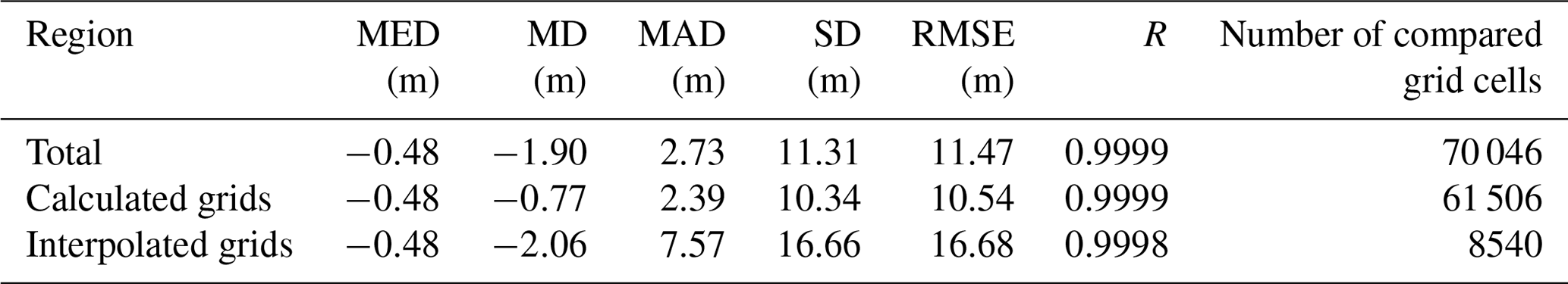
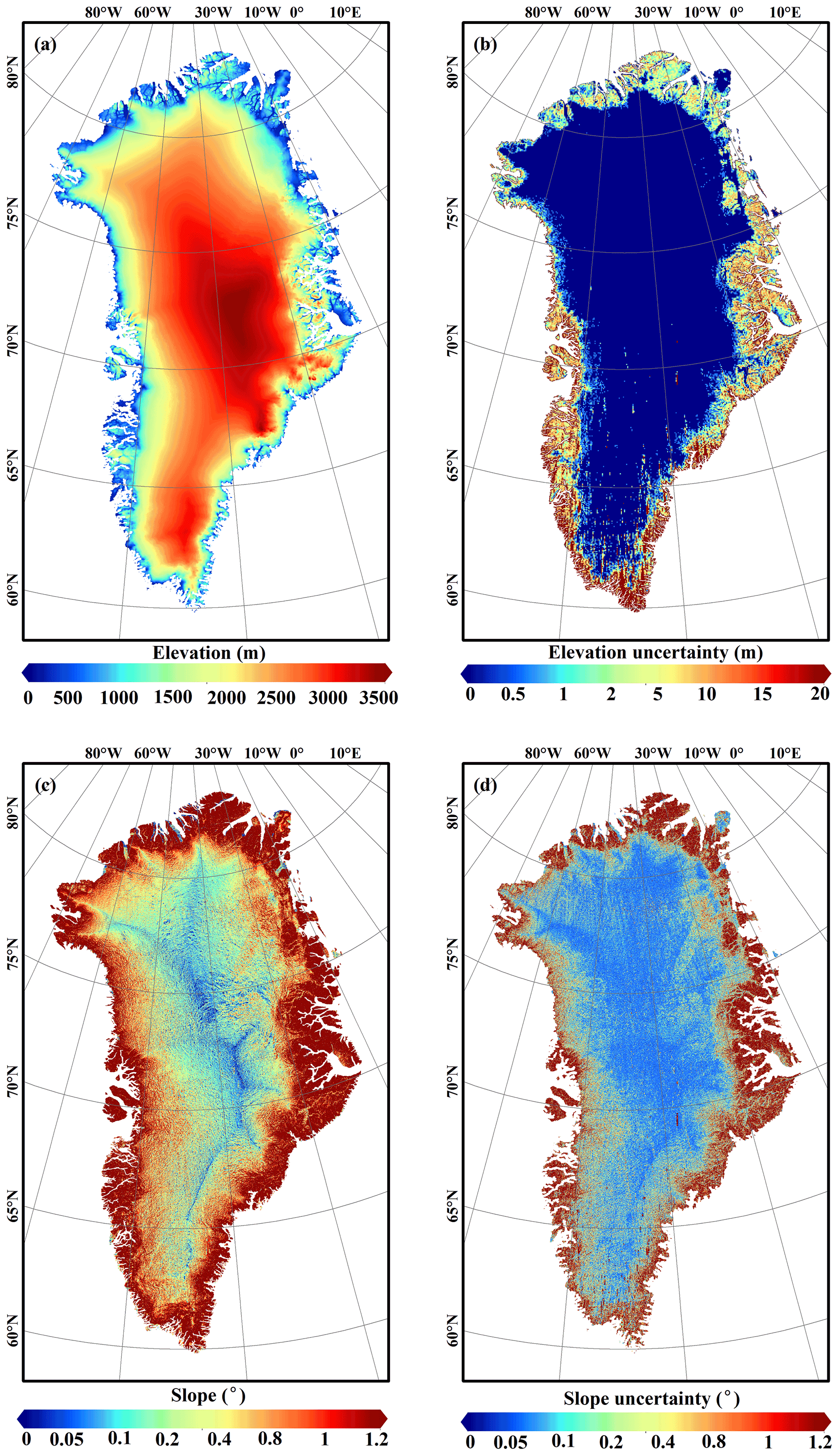
Figure 4(a) Elevation of the Greenland DEM calculated from 13 months of ICESat-2 footprints acquired between November 2018 and November 2019. (b) The elevation uncertainties. (c) Slope derived from the elevation map (a). (d) Slope uncertainty derived from the elevation map (b).
4.1 General attributes of ICESat-2 DEM
Approximately 33.00 %, 23.93 %, and 25.43 % of elevations were directly estimated from Greenland DEM at 500 m, 1 km, and 2 km resolutions, corresponding to the number of ICESat-2 footprints of 3.51×10⁸, 3.96×10⁸, and 4.50×10⁸, respectively. The ICESat-2 DEM shows the same pattern as the other published DEMs. The highest elevation appears in the ice sheets and shows a downward trend to the margins (Fig. 4a), and large topographic fluctuations occur on the outlet glaciers around the periphery of Greenland. Furthermore, the monthly elevation change rate was also obtained from spatiotemporal model fit; thus, the DEM for each month from November 2018 to November 2019 can be derived theoretically.
The DEM uncertainty and slope uncertainty show obvious latitude-dependent patterns. Larger values tend to be found at low latitudes, and this pattern may be related to the number of ICESat-2 measurement points in each grid cell. The uncertainty also presents an increasing trend from the interior to the margins, which is approximately less than 0.5 m in the inner ice sheet, and higher uncertainty of 2–5 m can be observed for the periphery of Greenland (Fig. 4b). The generated slope uncertainty is large at the edges, which is also concurrent with slopes exceeding 1∘ (Fig. 4c and d). The accuracy of satellite laser altimeters is affected by surface roughness, slope, and other environmental factors (Brunt et al., 2017). A flatter surface provides a more uniform reflection than a steeper surface of the measurement footprint, and more accurate height measurements of the original ICESat-2 footprints can be obtained in the low-slope regions, hence the higher accuracy of the ICESat-2 DEM.
Table 3Elevation differences between the ICESat-2 DEM and IceBridge data under different DEM resolutions.
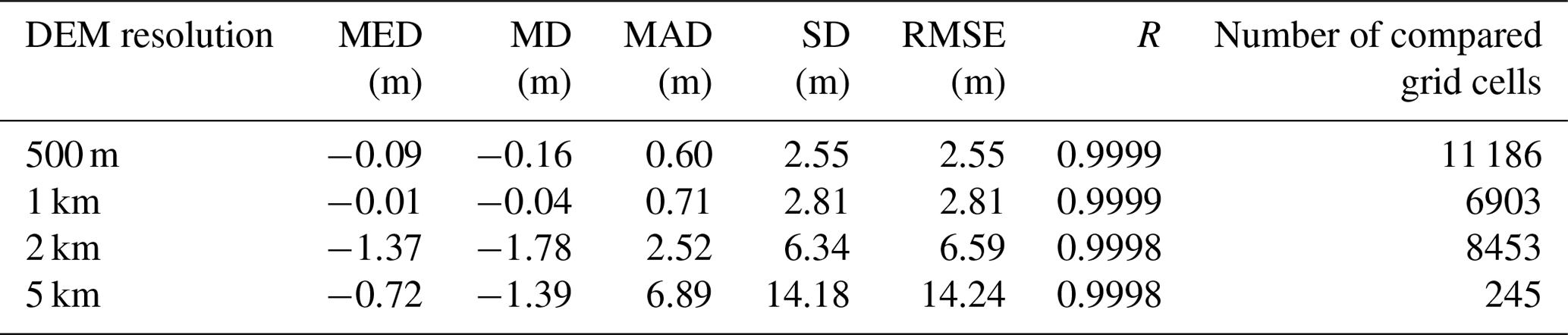
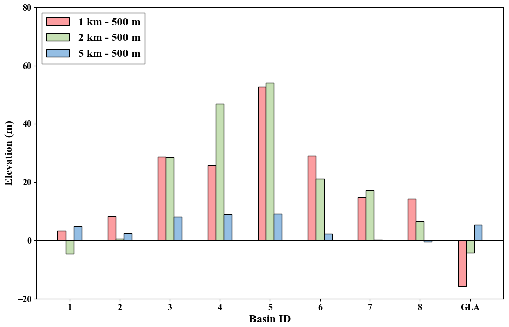
Figure 5Elevation differences of nine main regions under different resolutions, which are calculated by subtracting the 500 m DEM from the 1, 2, and 5 km DEMs through the overlapping grids of different DEMs. The color bar shows the mean elevation differences of these regions.
4.2 Evaluation of ICESat-2 DEM by comparing it with IceBridge data
The ICESat-2 DEM compares favorably to the IceBridge data (Fig. 5 and Table 2). The bias between Greenland DEM and IceBridge data in calculated grids is smaller than that of interpolated grids, which indicates that the elevations derived from model fit tend to be more accurate than those estimated from interpolation. Poorer performance in the interpolated grids is reasonable due to the low spatial correlation in the regions with large surface fluctuations such as the Greenland south margins. The application of four resolutions may add additional effects; i.e., different grid cell resolutions tend to present different elevation estimates; thus, DEMs of different resolutions (namely, 500 m, 1 km, 2 km, 5 km) were evaluated (Table 3). DEMs of 500 m and 1 km resolutions have similar performance, and DEMs of 2 and 5 km resolutions exhibit worse performances than those of 500 m and 1 km, but the biases of 2 and 5 km resolution DEMs are still smaller than the error in the interpolated grid. Hence, it is reasonable to apply different resolutions for posting the ICESat-2 DEM of 500 m resolution considering the differences between the calculated and interpolated grids.
Table 4Elevation differences between the ICESat-2 DEM and IceBridge data in different basins, calculated for all of Greenland and the calculated and interpolated grids. Basins with fewer than 30 grids were excluded. IceBridge data were acquired in May 2019.
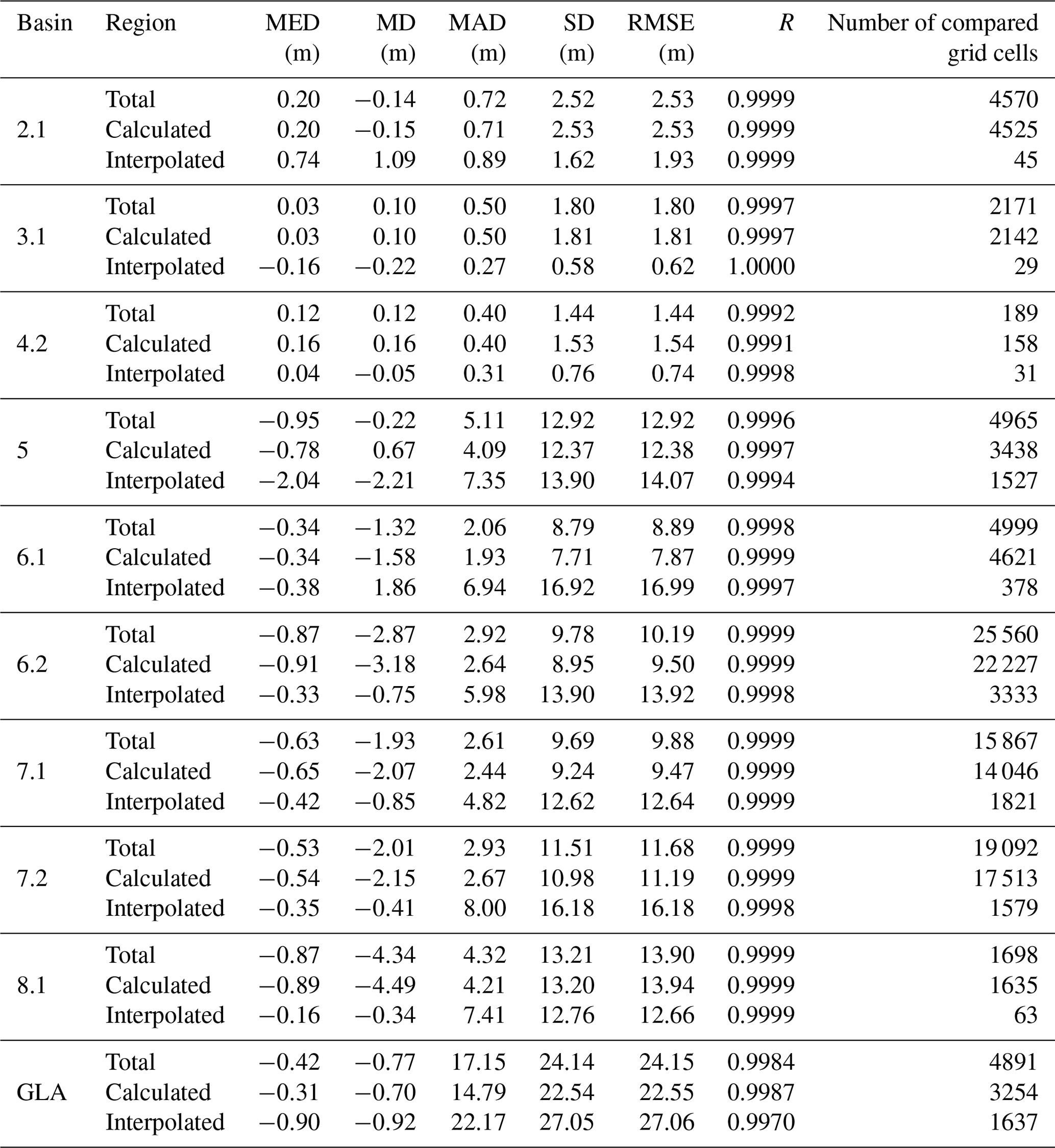
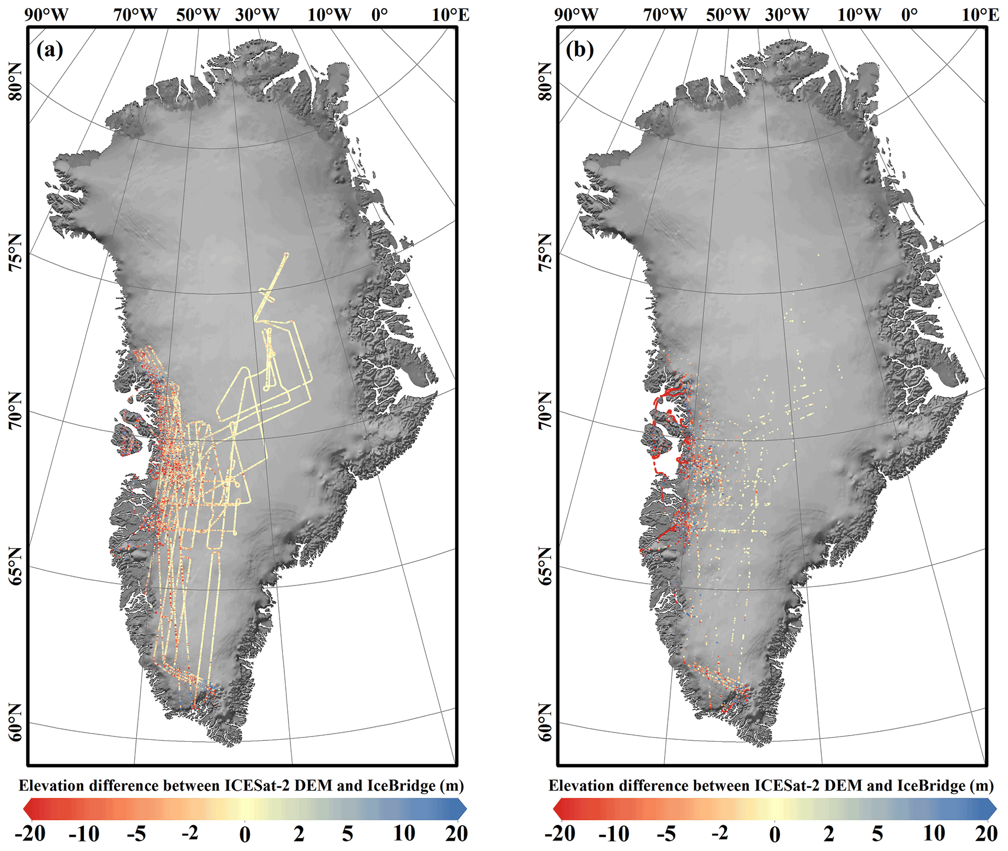
Figure 6Elevation difference calculated as IceBridge data subtracted from the new ICESat-2 DEM. (a) Calculated grids and (b) interpolated grids. IceBridge data were acquired in May 2019.
We also compared the accuracies according to the 10 basins covered by data from May 2019 (Table 4). The accuracy of the ICESat-2 DEM shows an apparent spatial trend in which better accuracy is observed in the north than in the south basins, and the pattern may be related to the small proportion of calculated grids in the southern basin and the application of DEMs with 2 and 5 km resolution. We calculated the mean elevation of main basins at four resolutions to further assess the effects of different spatial resolutions when generating the ICESat-2 DEM (Fig. 6). The calculated elevations were generally higher with increasing resolution, and the regions with the largest bias were concentrated in the low-latitude basins of Greenland. The small elevation difference for the GLA (glacier) region was possibly caused by the elevation being overestimated or underestimated on different glaciers due to the complex topography, and this uncertainty alleviated the elevation differences.
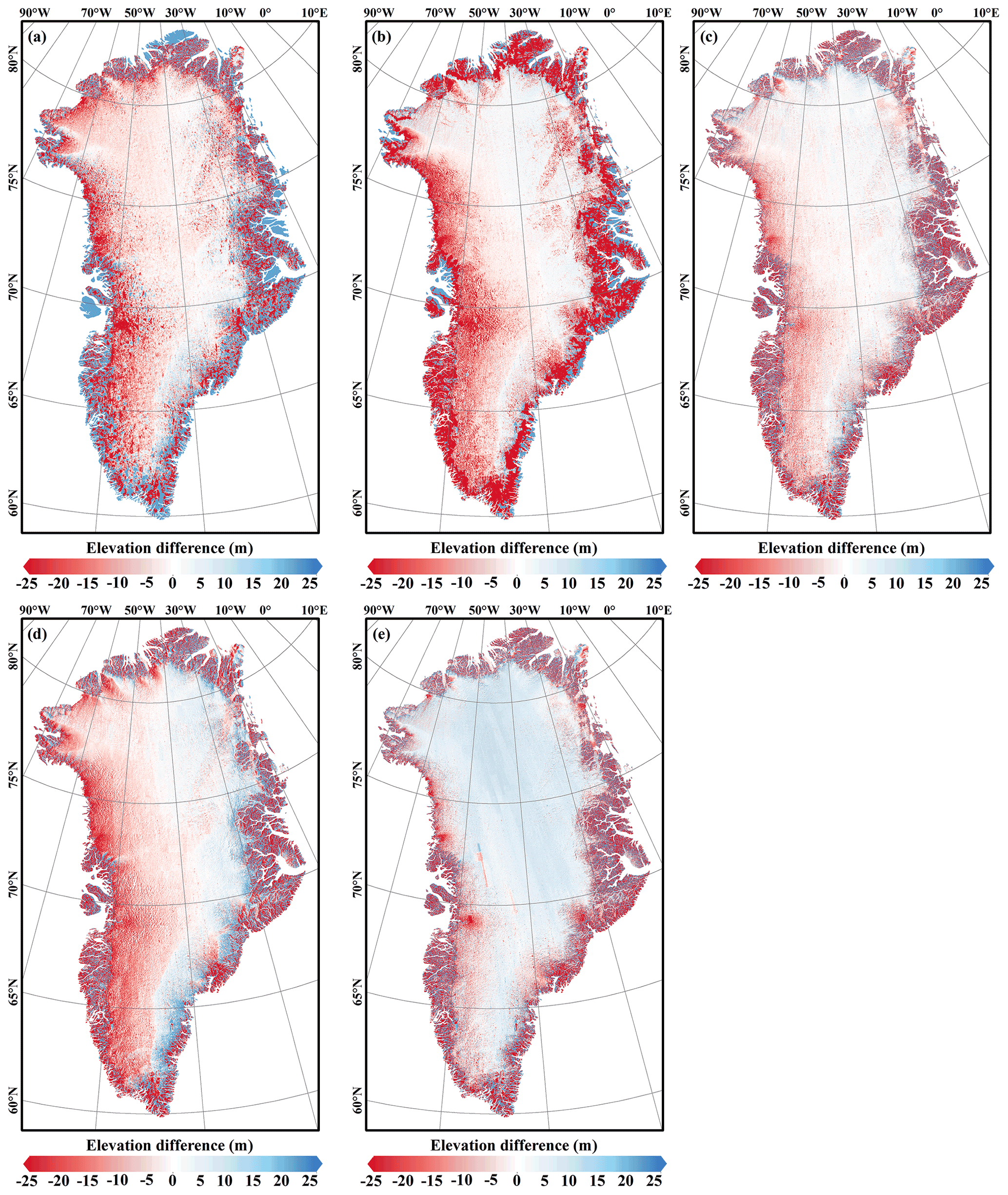
Figure 7Elevation differences calculated between the new ICESat-2 DEM and the other five published available DEMs: (a) ICESat DEM, (b) CryoSat-2 DEM, (c) 500 m ArcticDEM, (d) 1 km ArcticDEM, and (e) TanDEM-X. For each picture, the previously published DEM was resampled to 500 m, and the difference was calculated as the resampled DEM subtracted from the new ICESat-2 DEM.
There are still some differences between the ICESat-2 DEM and IceBridge data mainly due to the inconsistent coverages of the two datasets. It should be noted that the IceBridge data used for evaluation were distributed only at latitudes below 75∘ N, where the posted DEM was mostly derived from DEMs at coarse resolutions. The ICESat-2 DEM should have higher accuracy in regions beyond 75∘ N. Hence, these biases are acceptable because the evaluated value represents the upper bound of the ICESat-2 DEM bias, and the deviation should be smaller when considering the ICESat-2 DEM as a whole.
Table 5Elevation differences of the ICESat-2 DEM and other published DEMs with respect to IceBridge data. All of Greenland and the regions with elevations above 2000 m and below 2000 m were compared.
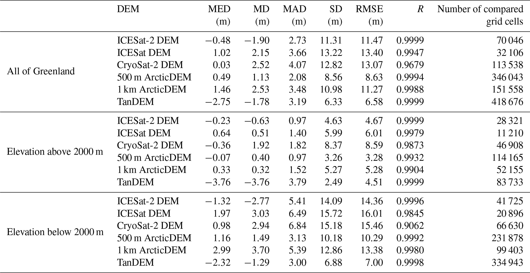
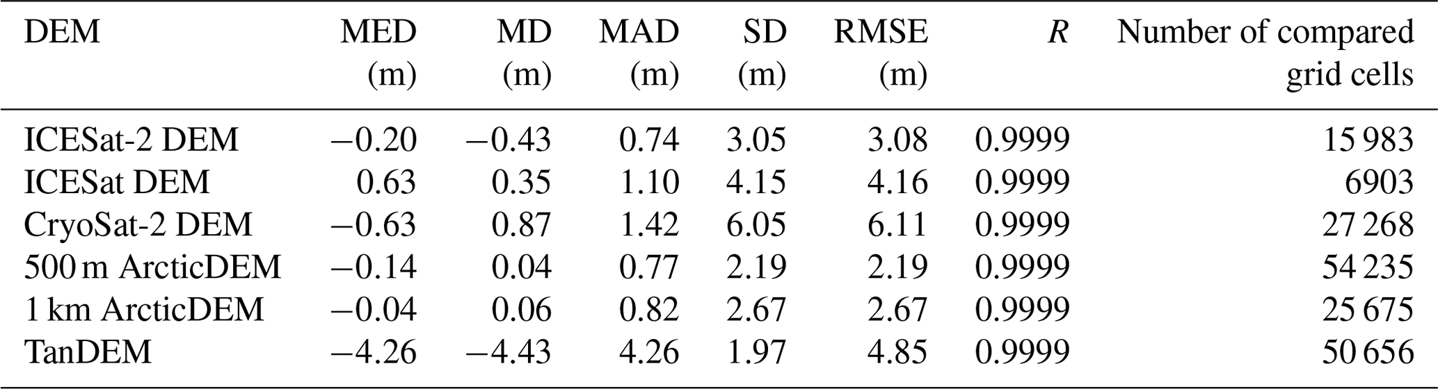
Table 6Elevation differences of the ICESat-2 DEM and other published DEMs with respect to IceBridge data in the regions which have little elevation change rate (−0.05–0.05 m yr−1).
The elevation differences between the new ICESat-2 DEM and the other five published DEMs show that DEMs usually perform better for low-slope regions (Fig. 7). The ICESat-2 DEM is generally close to that of the 500 m ArcticDEM except in complex terrains, which can prove the great reliability of the ICESat-2 DEM. In particular, significant positive values can be seen in the elevation difference between the ICESat-2 DEM and TanDEM on the Greenland ice sheet, which is assumed to be caused by X-band penetration into the snowpack. All the difference maps show significant negative values in the Jakobshavn Isbrae Glacier, which experienced the greatest loss of the Greenland ice sheet (Smith et al., 2020). This phenomenon may reflect the real elevation changes during different DEM acquisition times.
In this study, we used only IceBridge data that overlapped with the corresponding DEM period to evaluate all DEMs' vertical accuracies for all of Greenland and areas with small elevation changes (−0.05–0.05 m yr−1) (Smith et al., 2020). Results show that the ICESat-2 DEM showed significant improvements in accuracy compared with other altimeter-derived DEMs, and it is also comparable to DEMs derived from stereophotogrammetry and interferometry. Compared with the ICESat DEM derived from the 6.9×10⁶ footprints and the CryoSat-2 DEM derived from the 7.5×10⁶ footprints, approximately 80 times as many data points were used to generate the DEM; thus, the finer resolution of 500 m and higher accuracies can be obtained (Tables 5 and 6). The ICESat-2 DEM has the best performance with regard to the parameters except for the MED of the CryoSat-2 DEM. Contrary to expectations, there is no elevation underestimation in the CryoSat-2 DEM possibly because slope and topographic corrections have been performed. TanDEM has less bias in the coastal region, and this is possibly caused by ICESat data having been used to calibrate the raw DEMs there (Wessel et al., 2016). Although model-based or empirical models can, to some extent, correct the penetration bias (Abdullahi et al., 2019), such correction in the ice sheet is generally restricted to the regional scope (Wessel et al., 2021); thus, significant elevation underestimations cannot be corrected and still exist.
Table 7Elevation differences of the ICESat-2 DEM and 500 m ArcticDEM with respect to IceBridge data in all of Greenland and the stable regions which have a small elevation change rate (−0.05–0.05 m yr−1).
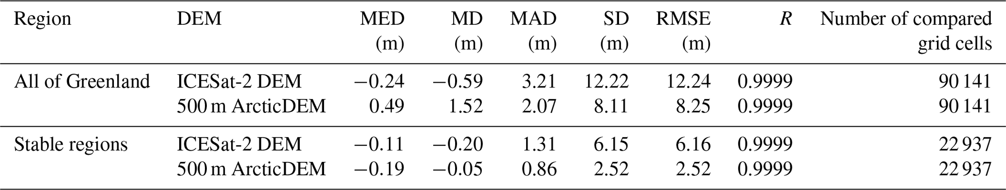
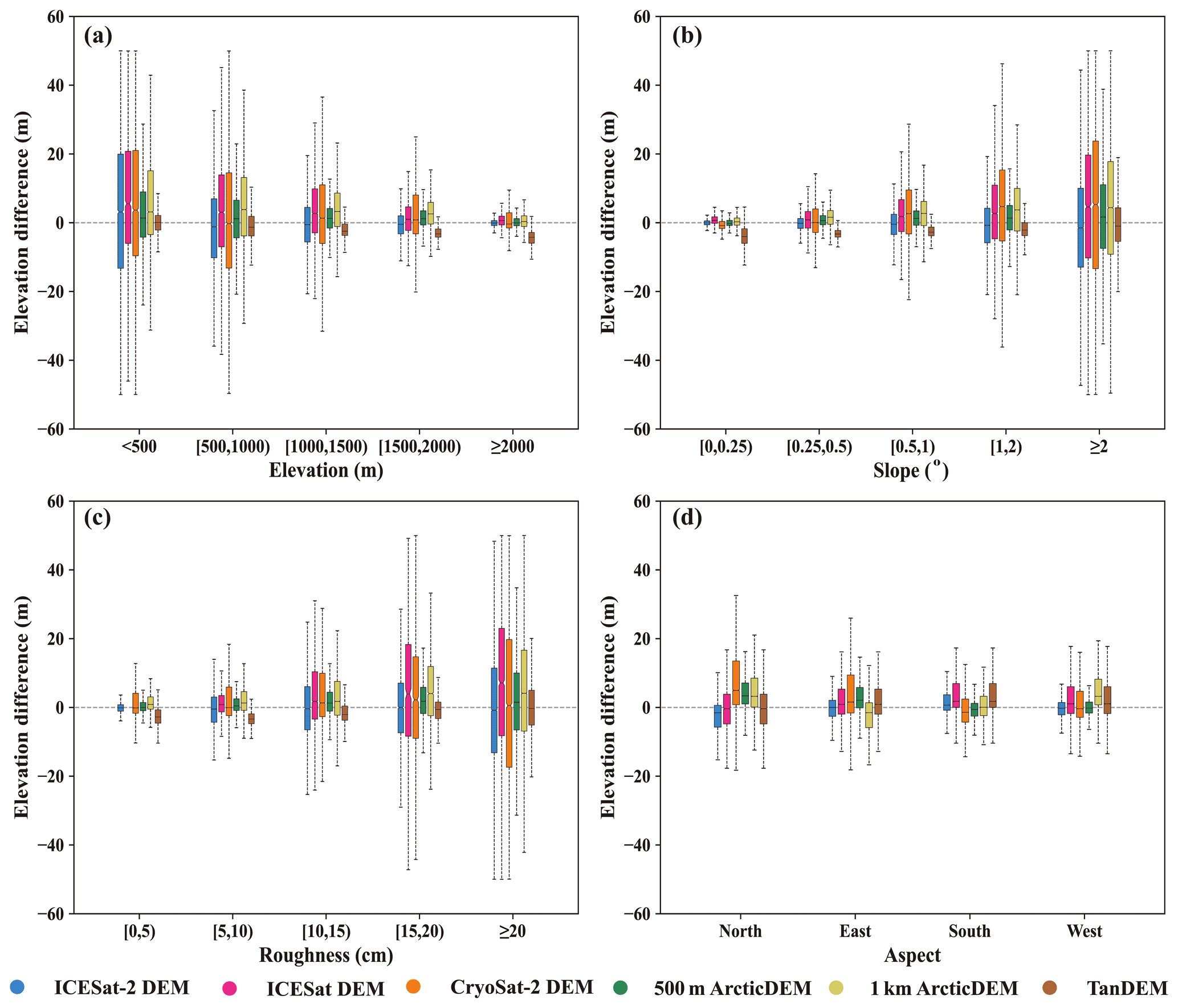
Figure 8Elevation differences between different DEMs and IceBridge data under different terrain conditions: (a) elevation, (b) slope, (c) roughness, and (d) aspect. The solid black lines near the box centers denote median values of elevation differences, the upper and lower boundaries of each box denote upper and lower quartiles (Q1 and Q3), the length means the interquartile range (IQR), and the top and bottom lines denote the range [Q1–1.5 IQR–Q3 + 1.5 IQR].
The accuracy of the ICESat-2 DEM is higher than the 1 km ArcticDEM. The comparison of 500 m ArcticDEM and ICESat-2 DEM using the IceBridge of the year 2018 can draw the same conclusion that the performance of the ICESat-2 DEM is comparable to the 500 m ArcticDEM (Table 7). The MAD, SD, and RMSE are all larger than those of the 500 m ArcticDEM, and it is reasonable that stereophotogrammetry can generate more consistent elevation estimations at the regional scale than altimetry. Nevertheless, the ICESat-2 DEM is comparable to the 500 m ArcticDEM when slopes are less than 1∘, which includes approximately 70 % of Greenland. ICESat data were used to calibrate the ArcticDEM in both the horizontal and vertical directions to increase the accuracy of the ArcticDEM, but the actual changes in the ice surface introduce additional uncertainties because ICESat data predate the ArcticDEM by almost 10 years. Besides, systematic errors among the ArcticDEM's different sensors may also affect its accuracy (Candela, 2017).
The median differences in surface slope and roughness for these DEMs illustrate that all their elevation biases become larger with increasing slope and roughness with the exception of TanDEM (Fig. 8b and c). Larger elevation differences in high-slope regions are reasonable as satellite images have a much finer original spatial resolution (2 m) than ICESat-2. Furthermore, DEMs generated by stereo pairs have obvious directivity in terms of surface aspect (Fig. 8d). The accuracy on the north slope is significantly lower mainly due to the poor illumination condition of the images in the north direction.
The elevation and elevation uncertainty maps of Greenland can be downloaded from the National Tibetan Plateau/Third Pole Environment Data Center, Institute of Tibetan Plateau Research, Chinese Academy of Sciences at https://doi.org/10.11888/Geogra.tpdc.271336 (Fan et al., 2021).
A new digital elevation model of Greenland was provided based on the ICESat-2 observations acquired from November 2018 to November 2019. The DEM was posted at a modal resolution of 500 m. A total of 98 % of the grids were directly derived from a model fit method, and an additional 2 % were interpolated by the kriging method. The application of different resolutions can reduce the number of interpolated grids and bias in the elevation estimation. Compared with spatiotemporally matched elevation measurements from the IceBridge data, we estimated the uncertainty with a median difference of −0.48 m for all of Greenland, which represents the upper bound of the ICESat-2 DEM bias. The accuracy of the ICESat-2 DEM shows an apparent spatial trend, and better accuracy can be observed in the northern basins than in the southern basins owing to the denser coverage of ICESat-2 tracks in the high-latitude regions.
Compared with other published Greenland DEMs, i.e., the ICESat DEM, CryoSat-2 DEM, 1 km ArcticDEM, 500 m ArcticDEM, and TanDEM, the ICESat-2 DEM maintains great accuracy stability under various topographic conditions. The ICESat-2 DEM is superior to the previous satellite-altimeter-derived DEMs in both spatial resolution and elevation accuracy. Smaller elevation differences between the ICESat-2 DEM and DEMs derived from stereophotogrammetry and interferometry can imply the reliability of the ICESat-2 DEM. Although the uncertainties in the ICESat-2 DEM are affected by the ICESat-2 measurements themselves, and the DEM in the low-latitude regions was derived from the results of coarse spatial resolution, the specific time-stamped ICESat-2 DEM can benefit studies of elevation change and mass balance in Greenland. More ICESat-2 data can be used to generate DEMs with higher resolution as more ICESat-2 observations become available, especially in the southernmost glaciers.
YF performed the DEM generation and wrote the manuscript. CQK contributed to the conception of the study and supervised the work. XS contributed to the discussion and advised on the comparison with IceBridge data. All authors contributed to the discussion of the results and to the improvement of the manuscript.
The contact author has declared that neither they nor their co-authors have any competing interests.
Publisher's note: Copernicus Publications remains neutral with regard to jurisdictional claims in published maps and institutional affiliations.
This article is part of the special issue “Extreme environment datasets for the three poles”. It is not associated with a conference.
This work is supported by the Program for National Natural Science Foundation of China (grant no. 41830105). The ICESat-2 data were obtained from the National Snow and Ice Data Center (http://nsidc.org, last access: 23 March 2021). We also thank the High Performance Computing Center, Nanjing University, for the computing support.
This research has been supported by the National Natural Science Foundation of China (grant no. 41830105).
This paper was edited by Xin Li and reviewed by two anonymous referees.
Abdullahi, S., Wessel, B., Huber, M., Wendleder, A., and Kuenzer, C.: Estimating Penetration-Related X-Band InSAR Elevation Bias: A Study over the Greenland Ice Sheet, Remote Sens., 11, 2903, https://doi.org/10.3390/rs11242903, 2019.
Bamber, J. L., Gomez-Dans, J. L., and Griggs, J. A.: A new 1 km digital elevation model of the Antarctic derived from combined satellite radar and laser data – Part 1: Data and methods, The Cryosphere, 3, 101–111, https://doi.org/10.5194/tc-3-101-2009, 2009.
Bamber, J. L., Griggs, J. A., Hurkmans, R. T. W. L., Dowdeswell, J. A., Gogineni, S. P., Howat, I., Mouginot, J., Paden, J., Palmer, S., Rignot, E., and Steinhage, D.: A new bed elevation dataset for Greenland, The Cryosphere, 7, 499–510, https://doi.org/10.5194/tc-7-499-2013, 2013.
Brunt, K. M., Hawley, R. L., Lutz, E. R., Studinger, M., Sonntag, J. G., Hofton, M. A., Andrews, L. C., and Neumann, T. A.: Assessment of NASA airborne laser altimetry data using ground-based GPS data near Summit Station, Greenland, The Cryosphere, 11, 681–692, https://doi.org/10.5194/tc-11-681-2017, 2017.
Brunt, K. M., Neumann T. A., and Smith B. E.: Assessment of ICESat-2 Ice Sheet Surface Heights, Based on Comparisons Over the Interior of the Antarctic Ice Sheet, Geophys. Res. Lett., 46, 13072–13078, https://doi.org/10.1029/2019GL084886, 2019.
Candela, S. G.: ArcticDEM Validation and Accuracy Assessment, AGU Fall Meeting, New Orleans, USA, 11–15 December 2017, 40260, https://agu.confex.com/agu/fm17/meetingapp.cgi/Paper/240260 (last access: 20 October 2021), 2017.
Dehecq, A., Millan, R., Berthier, E., Gourmelen, N., Trouvé, E., and Vionnet, V.: Elevation changes inferred from TanDEM-X data over the Mont-Blanc area: impact of the X-band interferometric bias, IEEE J. Sel. Top. Appl. Earth Obs. Remote Sens., 9, 3870–3882, https://doi.org/10.1109/JSTARS.2016.2581482, 2016.
DiMarzio, J. P.: GLAS/ICESat 1 km Laser Altimetry Digital Elevation Model of Greenland, Version 1, NASA National Snow and Ice Data Center Distributed Active Archive Center [data set], Boulder, Colorado USA, https://doi.org/10.5067/FYMKT3GJE0TM, 2007.
Fan, Y., Ke, C., and Shen, X.: A new Greenland digital elevation model derived from ICESat-2, National Tibetan Plateau Data Center [data set], https://doi.org/10.11888/Geogra.tpdc.271336, 2021.
Helm, V., Humbert, A., and Miller, H.: Elevation and elevation change of Greenland and Antarctica derived from CryoSat-2, The Cryosphere, 8, 1539–1559, https://doi.org/10.5194/tc-8-1539-2014, 2014.
Horn, B. K. P.: Hill shading and the reflectance map, Proceedings of the IEEE, 69, 14–47, https://doi.org/10.1109/PROC.1981.11918, 1981.
Howat, I. M., Negrete, A., and Smith, B. E.: The Greenland Ice Mapping Project (GIMP) land classification and surface elevation data sets, The Cryosphere, 8, 1509–1518, https://doi.org/10.5194/tc-8-1509-2014, 2014.
Korona, J., Berthier, E., Bernard, M., Remy, F., and Thouvenot, E.: SPIRIT. SPOT 5 stereoscopic survey of Polar Ice: Reference Images and Topographies during the fourth International Polar Year (2007–2009), ISPRS J. Photogramm. Remote Sens., 64, 204–212, https://doi.org/10.1016/j.isprsjprs.2008.10.005, 2009.
Korsgaard, N. J., Nuth, C., Khan, S. A., Kjeldsen, K. K., Bjork, A. A., Schomacker, A., and Kjaer, K. H.: Digital elevation model and orthophotographs of Greenland based on aerial photographs from 1978–1987, Sci. Data, 3, 15, https://doi.org/10.1038/sdata.2016.32, 2016.
Krabill, W., Hanna, E., Huybrechts, P., Abdalati, W., Cappelen, J., Csatho, B., Frederick, E., Manizade, S., Martin, C., Sonntag, J., Swift, R., Thomas, R., and Yungel, J.: Greenland Ice Sheet: Increased coastal thinning, Geophys. Res. Lett., 31, 4, https://doi.org/10.1029/2004gl021533, 2004.
Kurtz, N. T., Farrell, S. L., Studinger, M., Galin, N., Harbeck, J. P., Lindsay, R., Onana, V. D., Panzer, B., and Sonntag, J. G.: Sea ice thickness, freeboard, and snow depth products from Operation IceBridge airborne data, The Cryosphere, 7, 1035–1056, https://doi.org/10.5194/tc-7-1035-2013, 2013.
Markus, T., Neumann, T., Martino, A., Abdalati, W., Brunt, K., Csatho, B., Farrell, S., Fricker, H., Gardner, A., Harding, D., Jasinski, M., Kwok, R., Magruder, L., Lubin, D., Luthcke, S., Morison, J., Nelson, R., Neuenschwander, A., Palm, S., Popescu, S., Shum, C. K., Schutz, B. E., Smith, B., Yang, Y. K., and Zwally, J.: The Ice, Cloud, and land Elevation Satellite-2 (ICESat-2): Science requirements, concept, and implementation, Remote Sens. Environ., 190, 260–273, https://doi.org/10.1016/j.rse.2016.12.029, 2017.
Neumann, T. A., Martino, A. J., Markus, T., Bae, S., Bock, M. R., Brenner, A. C., Brunt, K. M., Cavanaugh, J., Fernandes, S. T., Hancock, D. W., Harbeck, K., Lee, J., Kurtz, N. T., Luers, P. J., Luthcke, S. B., Magruder, L., Pennington, T. A., Ramos-Izquierdo, L., Rebold, T., Skoo, J., and Thomas, T. C.: The Ice, Cloud, and Land Elevation Satellite-2 mission: A global geolocated photon product derived from the Advanced Topographic Laser Altimeter System, Remote Sens. Environ., 233, 16, https://doi.org/10.1016/j.rse.2019.111325, 2019.
Noh, M. J. and Howat, I. M.: Automated stereo-photogrammetric DEM generation at high latitudes: Surface Extraction with TIN-based Search-space Minimization (SETSM) validation and demonstration over glaciated regions, GISci. Remote Sens., 52, 198–217, https://doi.org/10.1080/15481603.2015.1008621, 2015.
Riel, B., Minchew, B., and Joughin, I.: Observing traveling waves in glaciers with remote sensing: new flexible time series methods and application to Sermeq Kujalleq (Jakobshavn Isbræ), Greenland, The Cryosphere, 15, 407–429, https://doi.org/10.5194/tc-15-407-2021, 2021.
Shen, X. Y., Ke, C. Q., Yu, X. N., Cai, Y., and Fan, Y. B.: Evaluation of Ice, Cloud, And Land Elevation Satellite-2 (ICESat-2) land ice surface heights using Airborne Topographic Mapper (ATM) data in Antarctica, Int. J. Remote Sens., 42, 2556–2573, https://doi.org/10.1080/01431161.2020.1856962, 2021.
Slater, T., Shepherd, A., McMillan, M., Muir, A., Gilbert, L., Hogg, A. E., Konrad, H., and Parrinello, T.: A new digital elevation model of Antarctica derived from CryoSat-2 altimetry, The Cryosphere, 12, 1551–1562, https://doi.org/10.5194/tc-12-1551-2018, 2018.
Smith, B., Fricker, H. A., Holschuh, N., Gardner, A. S., Adusumilli, S., Brunt, K. M., Csatho, B., Harbeck, K., Huth, A., Neumann, T., Nilsson, J., and Siegfried, M. R.: Land ice height-retrieval algorithm for NASA's ICESat-2 photon-counting laser altimeter, Remote Sens. Environ., 233, 17, https://doi.org/10.1016/j.rse.2019.111352, 2019.
Smith, B., Fricker, H. A., Gardner, A. S., Medley, B., Nilsson, J., Paolo, F. S., Holschuh, N., Adusumilli, S., Brunt, K., Csatho, B., Harbeck, K., Markus, T., Neumann, T., Siegfried, M. R., and Zwally, H. J.: Pervasive ice sheet mass loss reflects competing ocean and atmosphere processes, Science, 368, 1239, https://doi.org/10.1126/science.aaz5845, 2020.
Sutterley, T. C., Velicogna, I., Rignot, E., Mouginot, J., Flament, T., van den Broeke, M. R., van Wessem, J. M., and Reijmer, C. H.: Mass loss of the Amundsen Sea Embayment of West Antarctica from four independent techniques, Geophys. Res. Lett., 41, 8421–8428, https://doi.org/10.1002/2014gl061940, 2014.
Wessel, B., Bertram, A., Gruber, A., Bemm, S., and Dech, S.: A new high-resolution elevation model of Greenland derived from TanDEM-X, ISPRS Annals of Photogrammetry, Remote Sensing and Spatial Information Sciences, III-7, 9–16, https://doi.org/10.5194/isprsannals-III-7-9-2016, 2016.
Wessel, B., Huber, M., Wohlfart, C., Bertram, A., Osterkamp, N., Marschalk, U., Gruber, A., Reuß, F., Abdullahi, S., Georg, I., and Roth, A.: TanDEM-X PolarDEM 90 m of Antarctica: generation and error characterization, The Cryosphere, 15, 5241–5260, https://doi.org/10.5194/tc-15-5241-2021, 2021.
Wingham, D. J.: CryoSat: A mission to determine fluctuations in the Earth's ice fields, Igarss 2002: Ieee International Geoscience and Remote Sensing Symposium and 24th Canadian Symposium on Remote Sensing, Proceedings: Remote Sensing: Integrating Our View of the Planet, Ieee, New York, I–Vi, 1750–1752, 2002.
Xing, Z. Y., Chi, Z. H., Yang, Y., Chen, S. Y., Huang, H. B., Cheng, X., and Hui, F. M.: Accuracy Evaluation of Four Greenland Digital Elevation Models (DEMs) and Assessment of River Network Extraction, Remote Sens., 12, 24, https://doi.org/10.3390/rs12203429, 2020.
Zink, M., Bachmann, M., Brautigam, B., Fritz, T., Hajnsek, I., Krieger, G., Moreira, A., and Wessel, B.: TanDEM-X: The New Global DEM Takes Shape, Ieee Geosci. Remote Sens. Magazine, 2, 8–23, https://doi.org/10.1109/mgrs.2014.2318895, 2014.
Zwally, H. J., Schutz, B., Abdalati, W., Abshire, J., Bentley, C., Brenner, A., Bufton, J., Dezio, J., Hancock, D., Harding, D., Herring, T., Minster, B., Quinn, K., Palm, S., Spinhirne, J., and Thomas, R.: ICESat's laser measurements of polar ice, atmosphere, ocean, and land, J. Geodyn., 34, 405–445, https://doi.org/10.1016/s0264-3707(02)00042-x, 2002.