the Creative Commons Attribution 4.0 License.
the Creative Commons Attribution 4.0 License.
 | 21 Feb 2022
Airborne ultra-wideband radar sounding over the shear margins and along flow lines at the onset region of the Northeast Greenland Ice Stream
Steven Franke
Tobias Binder
John D. Paden
Nils Dörr
Tamara A. Gerber
Heinrich Miller
Dorthe Dahl-Jensen
Veit Helm
Daniel Steinhage
Ilka Weikusat
Frank Wilhelms
We present a high-resolution airborne radar data set (EGRIP-NOR-2018) for the onset region of the Northeast Greenland Ice Stream (NEGIS). The radar data were acquired in May 2018 with the Alfred Wegener Institute's multichannel ultra-wideband (UWB) radar mounted on the Polar 6 aircraft. Radar profiles cover an area of ∼24 000 km2 and extend over the well-defined shear margins of the NEGIS. The survey area is centered at the location of the drill site of the East Greenland Ice-Core Project (EastGRIP), and several radar lines intersect at this location. The survey layout was designed to (i) map the stratigraphic signature of the shear margins with radar profiles aligned perpendicular to ice flow, (ii) trace the radar stratigraphy along several flow lines, and (iii) provide spatial coverage of ice thickness and basal properties. While we are able to resolve radar reflections in the deep stratigraphy, we cannot fully resolve the steeply inclined reflections at the tightly folded shear margins in the lower part of the ice column. The NEGIS is causing the most significant discrepancies between numerically modeled and observed ice surface velocities. Given the high likelihood of future climate and ocean warming, this extensive data set of new high-resolution radar data in combination with the EastGRIP ice core will be a key contribution to understand the past and future dynamics of the NEGIS. The EGRIP-NOR-2018 radar data products can be obtained from the PANGAEA data publisher (https://doi.pangaea.de/10.1594/PANGAEA.928569; Franke et al., 2021a).
- Article
(20354 KB) - Full-text XML
- BibTeX
- EndNote


The Northeast Greenland Ice Stream (NEGIS) efficiently drains a large area of the Greenland Ice Sheet and is a crucial component of the ice sheet mass balance (Fahnestock et al., 1993; Rignot and Mouginot, 2012). It extends from the central ice divide over more than 600 km towards the northeastern coast, where it discharges ice through the three marine-terminating glaciers (79∘ North glacier, Zachariae Isbræ, and Storstrømmen glacier). The currently prevailing hypothesis is that an anomaly of elevated geothermal heat flux (GHF) leads to extensive basal melting (Fahnestock et al., 2001) and induces ice flow. The GHF at the onset of NEGIS is the most important and, at the same time, most uncertain parameter in the representation of basal melt and the subglacial hydrology in ice flow models (Smith-Johnsen et al., 2020). However, the large gap between observed and modeled basal melt rates (Gerber et al., 2021; Zeising and Humbert, 2021; MacGregor et al., 2016; Buchardt and Dahl-Jensen, 2007) inside the ice stream and in the broader surroundings of the NEGIS onset raises questions about the real thermal state at the bed. The exceptionally high GHF proposed by Fahnestock et al. (2001) would be non-compatible with known geological processes (Jóhannesson et al., 2020; Blackwell and Richards, 2004). Therefore, Bons et al. (2021) raise the question of how fast flow at the NEGIS onset is possible without an extraordinarily high basal heat flux and melt rates.
Unlike other ice streams in Greenland, the NEGIS lacks an extensive overdeepened bed and thus lateral topographic constraints (Joughin et al., 2001; Franke et al., 2020). The ice stream more or less symmetrically broadens along flow, as more ice is dragged through the shear margins (Fahnestock et al., 2001; Joughin et al., 2001). Subglacial water routing in combination with subglacial till deformation seems to be a further controlling mechanism of ice flow at the onset of the NEGIS (Keisling et al., 2014; Christianson et al., 2014). The outlet area is characterized by an overdeepened basin covered with unconsolidated sediments (Joughin et al., 2001; Bamber et al., 2013). Ice thinning as a consequence of increasing oceanic water temperatures around Greenland could thus potentially be transmitted far upstream (Christianson et al., 2014), and changes in the hydropotential might have significant effects on the ice stream geometry. The high susceptibility of NEGIS to marine-triggered discharge and the expected increase in ocean water temperatures in the years to come (Yin et al., 2011; Straneo et al., 2012) raises questions about the future ice stream stability and its effect on the Greenland Ice Sheet mass balance.
Large-scale ice flow models are essential tools to predict the future behavior of glaciers and ice sheets and are necessary to estimate future sea-level rise. Until today, these models fail to successfully simulate the NEGIS due to insufficient understanding of the key processes responsible for ice flow dynamics (Mottram et al., 2019; Shepherd et al., 2020), limiting the prediction accuracy. The East Greenland Ice-Core Project (EastGRIP; https://eastgrip.org, last access: 17 March 2021) aims to drill a deep ice core in the upstream area of the NEGIS, providing valuable insights into the climate record, basal properties, and ice flow history at the drill site. Ice cores provide in situ information on physical and chemical properties at high resolution but are limited as being a spatial point measurement. Hence, further geophysical techniques are required to extrapolate this information to obtain a complete picture of the ice dynamic properties.
Radio-echo sounding (RES) has long become a standard method in glaciology. The polar ice sheets as well as low-latitude glaciers and ice caps have extensively been covered by airborne (e.g., Steinhage et al., 1999; Schroeder et al., 2020) or ground-based (e.g., Pälli et al., 2002) RES surveys. The transmitted electromagnetic waves are sensitive to changes in dielectric permittivity and electrical conductivity and get reflected, scattered, or refracted at interfaces of dielectric contrasts in the medium they propagate (Fujita et al., 1999). The most common glaciological application is the sounding of ice thickness and bed topography (e.g., Hempel and Thyssen, 1992; Dahl-Jensen et al., 1997; Steinhage et al., 1999; Nixdorf and Göktas, 2001; Kanagaratnam et al., 2001; Franke et al., 2021b). Reflections within the ice column, or so-called internal reflection horizons (IRHs), are often caused by impurity layers of volcanic origin representing isochronous horizons (Millar, 1981). These provide valuable information on the ice flow regime and strain history (Vaughan et al., 1999; Jacobel et al., 1993; Hodgkins et al., 2000) and can be used to reconstruct past accumulation rates (e.g., Richardson et al., 1997; Nereson et al., 2000; Siegert and Hodgkins, 2000; Pälli et al., 2002; Nereson and Raymond, 2001), match ice cores from different locations (e.g., Jacobel and Hodge, 1995; Siegert et al., 1998; Hempel et al., 2000), and validate numerical ice flow models (e.g., Huybrechts et al., 2000; Baldwin et al., 2003). Further applications of RES include the detection of crevasses (e.g., Zamora et al., 2007; Eder et al., 2008; Williams et al., 2014), mapping of subglacial lakes and basal hydrology (e.g., Carter et al., 2007; Palmer et al., 2013; Young et al., 2016), identifying thermal regimes (e.g., Murray et al., 2000; Copland and Sharp, 2001), determining snow and firn genesis (e.g., Frezzotti et al., 2002), and obtaining information on the crystal orientation fabric (e.g., Matsuoka et al., 2003; Eisen et al., 2007; Jordan et al., 2020).
We present airborne radar data of the onset region of NEGIS recorded in 2018 by a multichannel ultra-wideband radar system. The data set consists of profiles oriented parallel and perpendicular to the ice flow direction. The high along-track and range resolution allows consistent isochrone tracing, providing insights into the three-dimensional structure of the ice stream. In combination with the EastGRIP ice core, this data set contributes to a better understanding of ice flow dynamics of the NEGIS. In our paper, we introduce the study site and survey design. Furthermore, we describe the radar data processing and the respective data products. The data are freely available from the PANGAEA data publisher (https://doi.pangaea.de/10.1594/PANGAEA.928569; Franke et al., 2021a).
In May 2018, we recorded radar data in the vicinity of the drill site of the EastGRIP ice core. An area of ∼24 000 km2 was mapped, with 7494 km of radar profiles along flow lines and perpendicular to ice flow (Fig. 1). The survey region extends ∼150 km upstream and downstream of the EastGRIP drill site and ranges from the central part of the ice stream up to 50 km beyond the shear margins. In our survey region, the ice stream accelerates from ∼10 to more than 80 m a−1 and widens from ∼15 to ∼55 km. The radar data also cover the transition in the position of the shear margin as well as strongly folded internal stratigraphy outside of the ice stream (see Fig. 1). Figure 1b and c show the locations of radar profiles in relation to the ice surface velocity. Profiles extending perpendicular to ice flow have a spacing of 5 km in the region close to the drill site and 10 km further up- and downstream. Along-flow profiles either follow flow lines, which in some cases pass through the shear margins, or are constantly located inside the ice stream. Other profiles are oriented parallel to ice flow of the NEGIS but are located outside of the ice stream.
The ice thickness in our survey region ranges from 2059 to 3092 m and shows, on average, a gradual decrease in thickness from the upstream to the downstream part (Franke et al., 2020, 2019). An analysis of the bed topography, basal roughness, and bed return echoes by Franke et al. (2021c) shows that our survey area can be divided into two different morphological regimes. The upstream part (upstream of EastGRIP) is characterized by a narrow ice stream width with accelerating ice flow velocity, a smooth bed with elongated flow-parallel subglacial landforms, and a soft till layer at the base (Christianson et al., 2014). Downstream of EastGRIP, the ice stream widens, and we note an overall change to a rougher and more variable bed geomorphology. The ice stream widens up to 57 km, and ice flow velocity keeps constant and decreases locally (Franke et al., 2021c).
In the 2012 summer field season, a scientific consortium collected ground-based geophysical data (RES and seismic survey) as well as a shallow ice core (Vallelonga et al., 2014). Christianson et al. (2014) examined the ice–bed interface by means of radar and seismic data analysis. They found high-porosity, water-saturated till, which lubricates the ice stream base and most likely facilitates ice streamflow. Keisling et al. (2014) used the same radar data to analyze the internal radar stratigraphy and suggest that the basal hydrology controls the upstream portion of the NEGIS. By contrast, the downstream part is rather confined by the bed topography. Riverman et al. (2019a) and Riverman et al. (2019b) analyzed the shear margins in particular and observed an increased accumulation and enhanced firn densification in the upper ice column as well as wet elongated subglacial landforms at the bed. Furthermore Holschuh et al. (2019) use RES data to evaluate 3D thermomechanical models of the NEGIS. The authors highlight the complexity of the stagnant-to-streaming ice flow transition and provide insights into the englacial heat transport. Finally, a comprehensive chemical analysis of a 67 m deep firn core was conducted by Vallelonga et al. (2014). The results demonstrated that a deep ice core at this location has the potential to retrieve a reliable record of the Holocene and last glacial cycle.
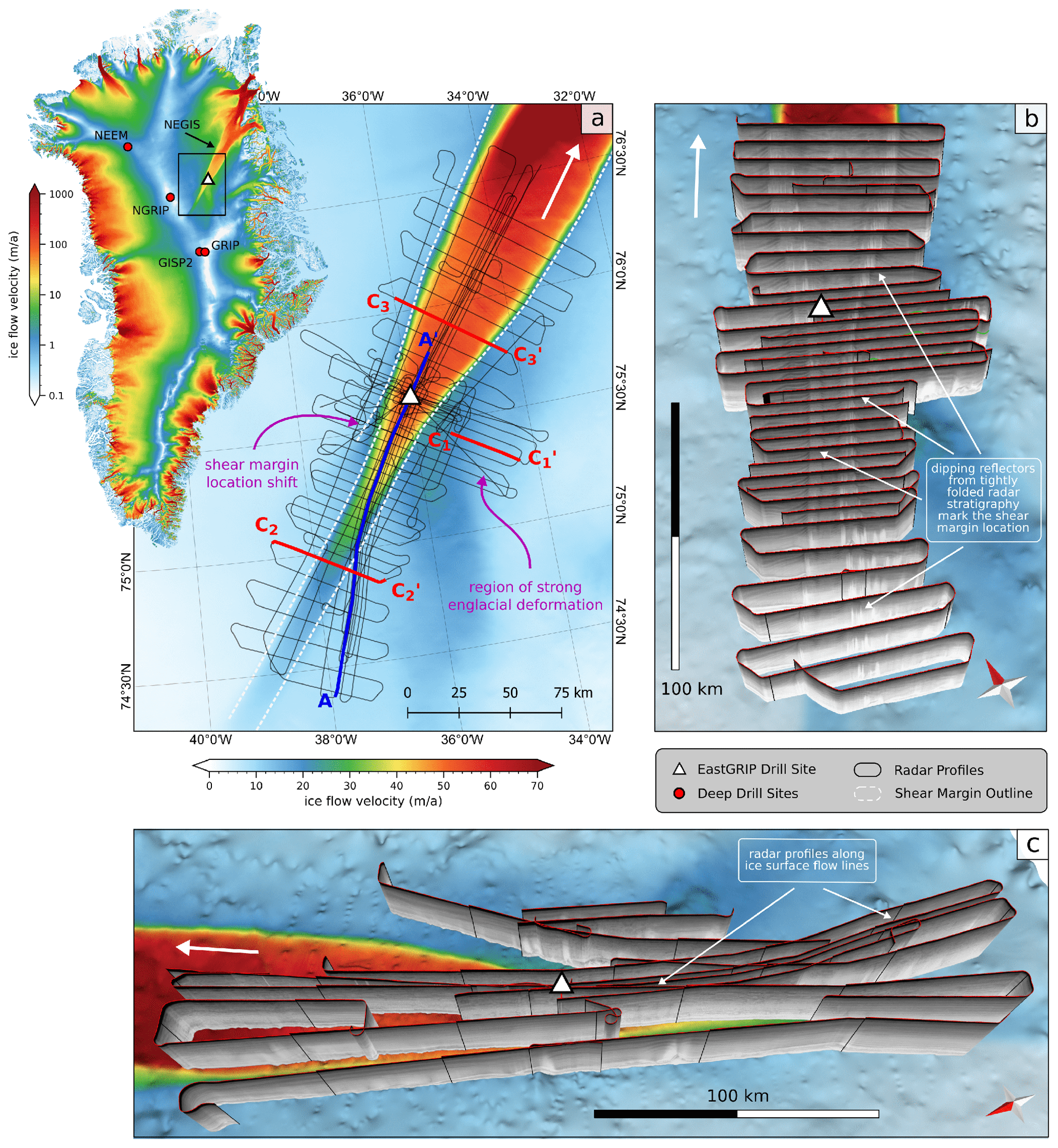
Figure 1Location of the EGRPI-NOR-2018 survey area in northeastern Greenland with the MEaSUREs ice surface velocity from Joughin et al. (2017) in the background. (a) The radar survey lines are centered at the EastGRIP drill site (white triangle) and extend up to 150 km upstream and downstream of the NEGIS. The locations of one along-flow radar section (Fig. 2; blue) and three cross-flow radar sections (Fig. 3; red) are shown in panel (a). The ice flow direction of the ice stream is indicated with a white arrow. Three-dimensional images of the cross-flow profiles and along-flow profiles are shown in (b) and (c), respectively. The radar sections are shown with a vertical exaggeration factor of z=10. The ice surface velocity (Joughin et al., 2017) is shown on a logarithmic scale (log10) for all of Greenland (upper left image) and on a linear scale for panels (a), (b), and (c). For panels (b) and (c) the ice surface velocity is projected on top of the bed topography model from Franke et al. (2020). The projection for all maps is WGS 84/NSIDC Sea Ice Polar Stereographic North (EPSG:3413).
3.1 Radar data acquisition
The ultra-wideband (UWB) airborne radar is a Multichannel Coherent Radar Depth Sounder (MCoRDS, version 5), which was developed at the Center for Remote Sensing of Ice Sheets (CReSIS) at the University of Kansas (Hale et al., 2016). It has an improved hardware design compared to predecessor radar depth sounders by CReSIS (Gogineni et al., 1998; Wang et al., 2015). The radar configuration deployed in 2018 consists of an eight-element radar array mounted under the Polar 6 Basler BT-67 aircraft's fuselage. The eight antenna elements function as transmit and receive channels using a transmit–receive switch. The total transmit power is 6 kW, and the radar can be operated within the frequency band of 150–600 MHz. The pulse repetition frequency (PRF) is 10 kHz, and the sampling frequency is 1.6 GHz. The characteristics of the transmitted waveform as well as the recording settings can be manually adjusted. We refer to the combined transmission–reception settings as waveforms in the following.
All profiles were recorded using linear frequency-modulated chirps in the frequency band of 180–210 MHz, antenna elements oriented with the E plane aligned with the along-track (HH polarization), and the transmit antenna beam pointed toward nadir. We used three alternating waveforms to increase the dynamic range of the system (see Table 1). Short pulses (1 µs) and low receiver gain of 11 dB are used to image the glacier surface, and longer pulses (3–10 µs) with higher receiver gain (48 dB) to image internal features and the ice base. Recorded traces were coherently pre-summed with zero-pi modulation in the hardware (Allen et al., 2005) to reduce the data rate and to increase signal-to-noise ratio (SNR), leading to a reduced effective PRF. The pre-sum factors were selected with regard to the pulse length of the respective waveform. To reduce range side lobes without losing much signal power, the transmitted and the pulse compression filter were amplitude-tapered using a Tukey window with a taper ratio of 0.08 (Li et al., 2013).
Before the data acquisition, the amplitude, phase, and time delay of the antenna elements were equalized during a test flight over open water during the transit to Greenland. During data acquisition, the position of the aircraft was determined by four NovAtel DL-V3 GPS receivers, which sample at 20 Hz. The GPS system operates with dual-frequency tracking so that the position accuracy can be enhanced during post-processing.
Table 1Acquisition parameters of the EGRIP-NOR-2018 radar campaign.
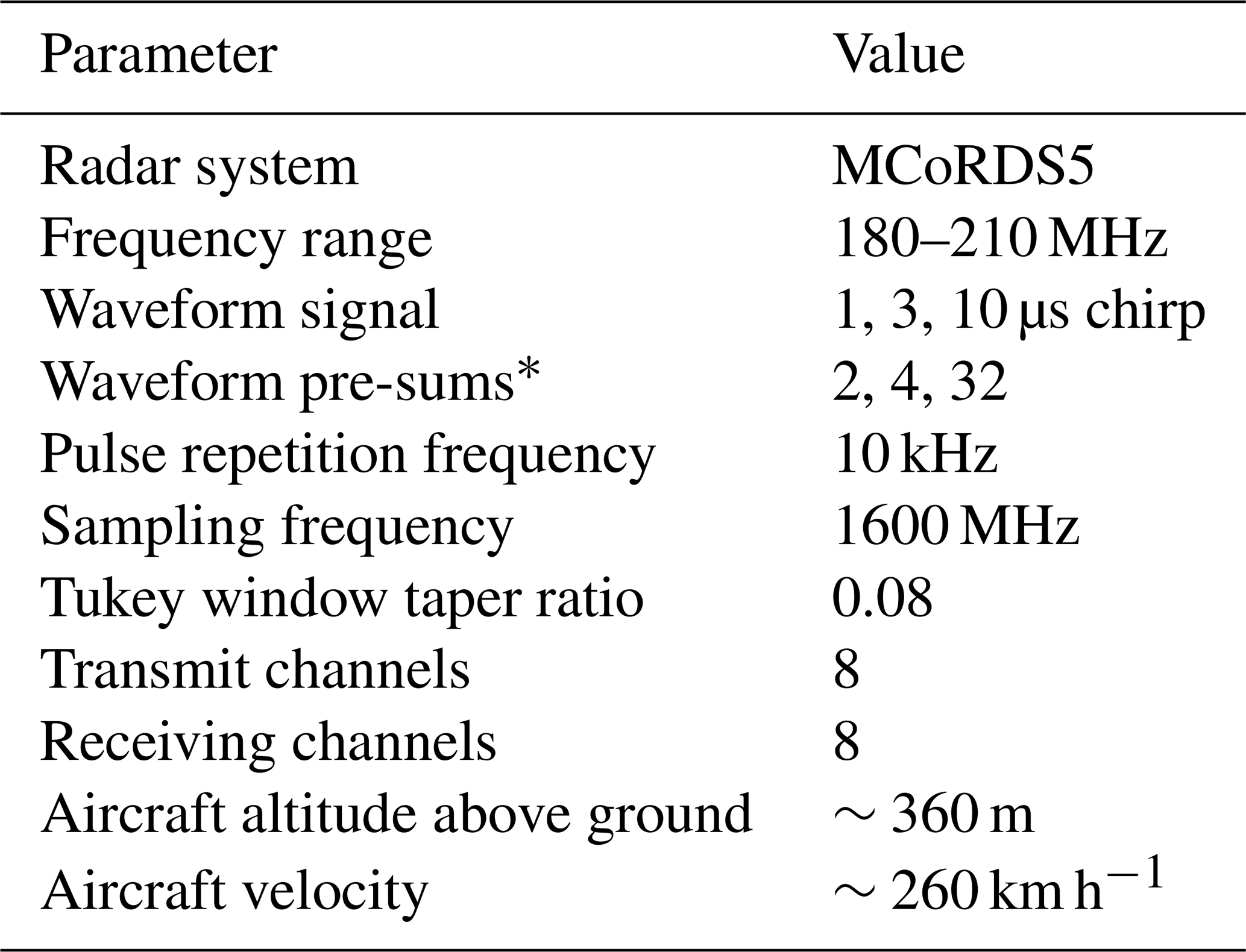
∗ Pre-sums are set for each waveform individually.
3.2 Radar data processing
The acquired data comprised a total of 24 total radargrams, each consisting of a pairwise combination of 1 of 8 receivers and 1 of 3 waveforms. The post-flight processing goal was to create single radargrams of the profiles covering the ice sheet from surface to base with high SNR, fine resolution, and high dynamic range. The main processing included pulse compression in the range dimension, synthetic aperture radar focusing in the along-track dimension, and array processing in the cross-track and elevation-angle dimension. Lastly, we vertically concatenated the radargrams of the three waveforms. The post-processing tools are implemented in the CReSIS Toolbox (CReSIS, 2020b).
At first, the recorded traces were pulse-compressed using a Tukey time domain weighting on the pulse- and frequency-domain-matched filtering with a Hanning window to reduce side lobes. For this purpose, the matched filter duplicates the transmitted waveforms based on the radar transmit settings.
Synthetic aperture radar (SAR) processing was carried out to focus the SAR radargrams in the along-track direction. The SAR processing is based on the fk (frequency–wavenumber) migration technique for layered media (Gazdag, 1978), which was adapted for radioglaciology (Leuschen et al., 2000). We used a two-layered velocity model with constant permittivity values for air (ϵair=1) and ice (ϵice=3.15). We consider the constant value of ϵice=3.15 to be justified since the uncertainties in the propagation velocity in the firn layer have a negligible effect on the fk migration. Furthermore, we use ϵice=3.15 to be consistent with the value used for processing of Operation Ice Bridge (OIB) data. The air–ice interface was tracked using quick-look imagery, which is generated using 20 coherent averages followed by 5 incoherent averages by an automated threshold tracker. Platform motion compensation is applied during averaging. The SAR aperture length at each pixel was chosen to create a fixed along-track resolution of 2.5 m. A requirement for the fk migration is a uniformly sampled linear trajectory of the receivers along the SAR aperture extent.
To estimate the flight trajectory we used Novatel OEM6 receivers at 20 Hz data rate. The precise point positioning (PPP) post-processed accuracy (commercial software package Waypoint 8.4) is estimated to be better than 3 cm for latitude and longitude and better than 10 cm for altitude. INS data were acquired by the onboard laser gyro inertial navigation system (Honeywell LASERREF V). Its accuracy is given to be better than 0.1∘ for pitch and roll and better than 0.4∘ for true heading (Honeywell product description). Changes in aircraft elevation, roll, pitch, and heading lead to phase errors in the migrated data and thus to decreased SNR and blurring. Processed GPS and INS data in high precision from the aircraft were used to correct these effects.
The motion compensation consisted of (1) uniformly resampling the data in along-track using a windowed sinc interpolation, (2) fitting lines to the resampled trajectory with the length of the SAR aperture, and (3) correcting any flight path deviations from the straight lines with phase shifts in the frequency domain.
After the along-track focusing, the channels were combined to increase the SNR and reduce the impact of surface clutter and off-nadir reflections. The delay-and-sum method allows for steering of the antenna array beam. The antenna array beam is steered toward nadir by coherently summing the data from each channel while accounting for the actual position of each measurement phase center. A total of 11 along-track averages (multilooking) are then performed to reduce speckle in the imagery.
Finally, the different waveform images were vertically combined to increase the dynamic range of the result. The two-way travel time (TWT) at which the radargrams are combined were chosen with regard to the pulse durations of the transmitted waveforms and the surface return in order to avoid saturation of the high-gain channels due to the strong surface return. For three-waveform collection with 1, 3, and 10 µs nadir waveforms, image 2 is combined with image 1 after 3 µs after the surface reflection and image 3 with image 2 10 µs after the surface return (see Fig. 5).
3.3 Resolution and uncertainty analysis
3.3.1 Range resolution
The theoretical range resolution after pulse compression is
where c denotes the speed of light in a vacuum, ϵr the real part of the ordinary relative permittivity, B the bandwidth of the transmitted chirp, and kt the windowing factor due to the frequency and time domain windows. For the bandwidth of 30 MHz, the theoretical range resolution in ice with ϵr=3.15 and kt=1.53 is 4.31 m.
In addition, to estimate the accuracy of a specific target (internal layer or bed return), we have to consider the RMS error in the dielectric constant (CReSIS, 2020a). Here we depend on the exact detection of the ice surface reflection, which is well constrained for our data.
To determine range resolution variability for the bed reflection for the radar data, we performed a crossover analysis of bed pick intersections (see Franke et al., 2020) and calculated the mean deviation hc. We consider an error on the order of 1 % for the dielectric constant for typical dry ice (Bohleber et al., 2012),
with the ice thickness T and a mean value for crossover deviation, hc. The full analysis of the range resolution of the bed reflection is documented in Franke et al. (2020) and shows a variability from 13 to 17 m.
3.3.2 Bed return resolution
A further parameter is the size of the area illuminated by the radar wave in the bed reflection signal. Here we consider a cross-track resolution for a typical rough surface σy. It is constrained by the pulse-limited footprint and depends on the Tukey and Hanning window parameters,
where H is the elevation of the aircraft over the ice surface. All EGRIP-NOR-2018 flights were performed at an aircraft elevation of ∼ 365 m above ground. When off-nadir clutter is visible in the radargrams, the cross-track resolution depends on the full beam width, βy, of the antenna array,
where λc is the wavelength at the center frequency, N is the number of array elements, and dy is the element spacing of the antennas. The cross-track resolution is now defined as
where ky is the approximate cross-track windowing factor for a Hanning window applied to a small cross-track antenna array.
For areas without signal layover, the cross-track footprint ranges between 300–350 m for an ice column of 2000–3000 m in our survey region (Franke et al., 2020). Where layover occurs, we have to consider Eq. (5) with a beam angle of ∼ 21∘. Here the cross-track resolution ranges between 800 and 1100 m.
The design of the EGRIP-NOR-2018 radar survey enables a detailed analysis of the bed and englacial stratigraphy: (i) along radar profiles which are parallel to the ice flow (Fig. 1c) and (ii) along radar profiles perpendicular to the ice flow, crossing the shear margins (Fig. 1b). In addition, several radar lines cover the location where the northern shear margin shifts its location (Fig. 1a) and an area southwest of EastGRIP where we observe patterns of strong internal ice deformation (location indicated in Fig. 1a).
In flow-parallel profiles, we observe three regimes showing different characteristics in the radar stratigraphy. Figure 2 shows a ∼200 km long flow-parallel radargram extending from the far upstream end outside of the NEGIS up to 30 km downstream of EastGRIP. The area outside of the ice stream at a distance of 0–60 km shows slightly folded internal layers, which have no connection to the local basal topography. Steeply dipping internal layers are characterized by a decrease in reflectivity with depth. The part of the profile which is crossing the shear zone (at 60–90 km distance) is characterized by tight folds in the internal layers, which extend almost up to the ice surface. The folds' apparent wavelength in profile direction depends on the intersection angle with respect to the shear margin orientation. Folds are tightest in profiles oriented ∼90∘ to the shear margin fold axis. We observe the best resolution of internal layers inside the ice stream, particularly in the lower part of the ice column. All distortions in the internal stratigraphy inside the ice stream seem to be related to the underlying bed.
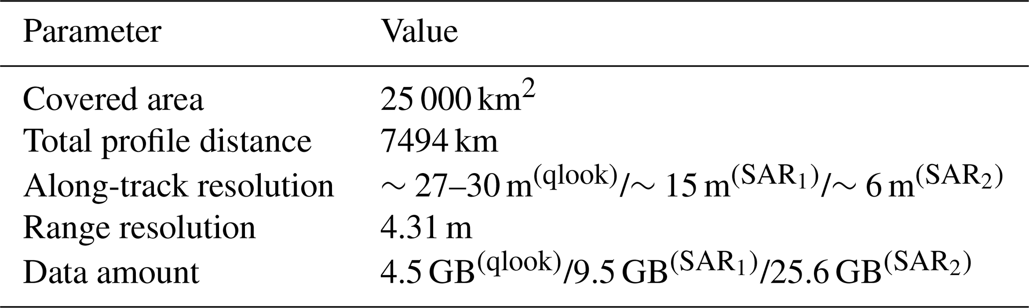
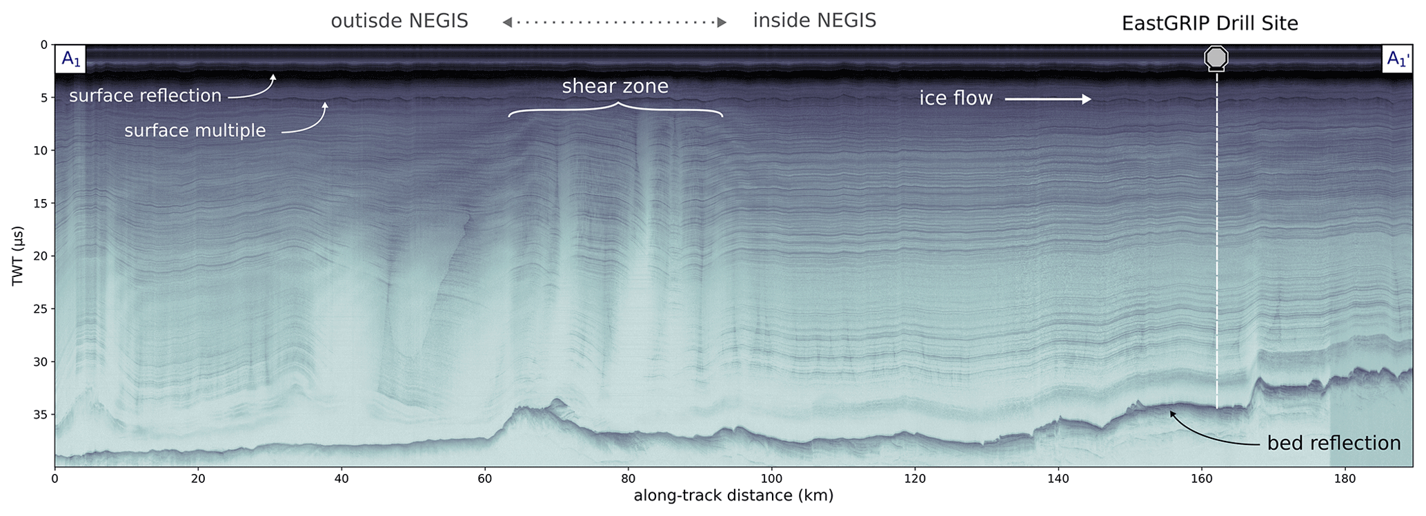
Figure 2Flow-parallel radar profile A composed of four frames: 20180512_01_001–004. The location is indicated in Fig. 1a and covers the area outside of the ice stream, the shear zone, and the ice stream's trunk. The position of the EastGRIP drill site is labeled and indicated with a vertical dashed white line.
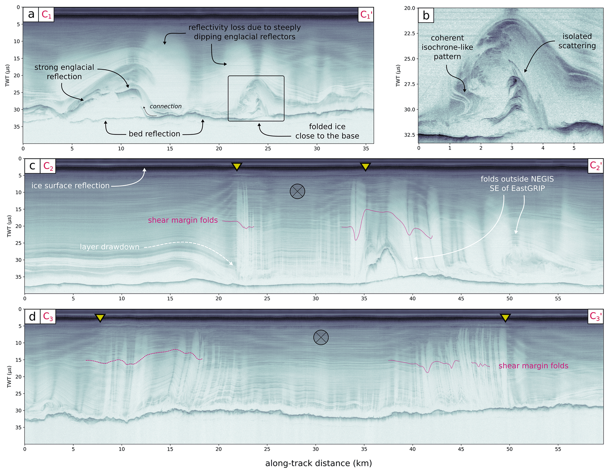
Figure 3Radar profiles , , and (frames 20180508_06_003, 20180511_01_007, and 20180514_01_011–012, respectively). The corresponding locations are shown in Fig. 1a. Panel (a) shows a profile located outside of the NEGIS, southeast of EastGRIP. A close-up of an anticline and other patterns of deformation are shown in panel (b), resembling the skeleton of a dead penguin. A slice through the ice stream in the upstream region is shown in panel (c) and a radar section further downstream in (d). The position of the shear margins (the maximum in the surface velocity gradient) is indicated with a yellow triangle and the folds in the shear margin areas with purple lines. The ice flow direction is into the page.
Radar profiles oriented perpendicular to ice flow show a strong imprint of NEGIS' dynamics. The most striking features are tight folds in the area of the shear margins. Bright stripes characterize them in the radargrams (e.g., Fig. 3), which represent a loss in return power due to steeply inclined internal reflectors (Holschuh et al., 2014; Keisling et al., 2014). The onset of this kind of folding starts at the shear zone's outer boundary (marked by yellow triangles in Fig. 3c and d). Depending on the ice stream's location and width, these folds can be traced towards the ice stream center for up to tens of kilometers, also towards locations where no shearing at the ice surface is observed. This becomes evident by comparing the upstream and farther-downstream radargram in Fig. 3c and d.
At several locations in flow-perpendicular radargrams we observe a drawdown of the radar stratigraphy towards the shear zone's outer margin (see Fig. 3c). The drawdown could be explained by temperate ice at the base (Franke et al., 2021c). Melting at the base at this location would be in agreement with subglacial hydrology modeling results by Riverman et al. (2019a), who suggest that melt out of sediments within the ice column potentially creates the subglacial bedforms they identified. In general, the stratigraphy of internal layers northwest of the NEGIS differs from the stratigraphy southeast of the NEGIS. The northwest is much more undisturbed than the southeast. A distinct example is shown in Fig. 3a and b. The stratigraphy is marked by long-wavelength anticlines and synclines with elevation differences of almost half of the ice column. In the anticlines' cores, we find strong englacial reflections, which have been misinterpreted before as bedrock (Franke et al., 2020). We note that some of the englacial reflections appear to be attached to the basal reflection (Fig. 3a). This could be an indication that the strong englacial reflection could be due to basal material (e.g., soft sediments) that was transported upwards by the folding process. Figure 3b shows that the deformation patterns in the anticline cores are very complex. Some of the reflection patterns (e.g., in Fig. 3b) result in connected structures similar to the isochrones in the upper part of the ice column. In addition, we find isolated patches with high reflectivity, which, however, do not show a coherent pattern (highlighted in Fig. 3b).
4.1 Data products
We offer three different data products of the EGRIP-NOR-2018 radar survey: (i) quick-looks (qlook), (ii) SAR-focused (SAR1), and (iii) SAR-focused with a large aperture (SAR2). The general data record properties are shown in Table 2, and detailed documentation can be found in the CReSIS MCoRDS documentation (https://data.cresis.ku.edu/, last access: 17 March 2021) and on the CReSIS Wiki website (https://ops.cresis.ku.edu/wiki/index.php/Main_Page, last access: 17 March 2021). In Fig. 4 we provide an overview of the differences between these three data products of the radargrams.
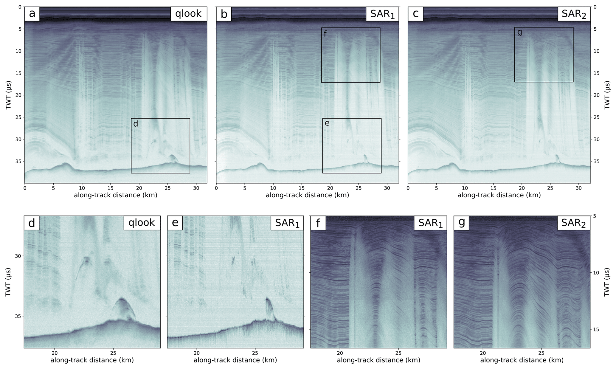
Figure 4Radargrams of a flow-perpendicular radar profile showing the three different data products: (a) quick-look (qlook) processed, (b) SAR-focused (SAR1), and (c) SAR-focused with a larger aperture (SAR2). The main difference between qlook and SAR1 is the focusing of signals via fk migration (d, e). In contrast to the default SAR focusing (f) a larger aperture enables a better resolution of steeply inclined internal layers (g).
4.1.1 qlook
This product uses unfocused synthetic aperture radar processing for each channel and assumes that all reflections arrive at the receiver from nadir. The data are coherently stacked in slow time, and no correction for propagation delay changes is applied. Here, no motion compensation is applied. Finally, the signals from all eight channels are averaged incoherently. The range resolution is the same as for all other products. The trace spacing is ∼27–30 m.
4.1.2 SAR with default settings (SAR1)
This data product uses focused synthetic aperture radar processing (fk migration) on each channel individually. The SAR processing requires a uniformly sampled linear trajectory along the extent of the SAR aperture. Motion compensation is applied using high-precision processed GPS and INS data from the aircraft. The direction of arrival is estimated by delay-and-sum beam forming to combine the channels. A Hanning window is applied in the frequency domain to suppress side lobes. This product is comparable to the CReSIS standard data product. The trace spacing is ∼15 m.
4.1.3 SAR with wider angular range (SAR2)
By processing at a finer SAR resolution, the SAR processor uses scattered energy from a wider angular range around nadir to form the image. Since the angle of scattered returns from a specular internal layer is proportional to the internal layer slope, the SAR processor's increased sensitivity to larger angle returns translates to an increased sensitivity to layers with larger slopes. We achieve a better resolution of steeply inclined internal reflectors by changing the along-track resolution before SAR processing to 1 m (, whereas the default setting is σx=2.5); 1 m is not the smallest possible value for processing but is within the limit to achieve a sufficiently high SNR. The SNR is smaller for larger angles because the range to the target increases for greater angles, which leads to additional signal loss (spherical spreading loss and additional signal attenuation in ice). The differences between radargrams processed with σx=1 and 2.5 are shown in Fig. 4. The final trace spacing is ∼6 m.
4.1.4 Individual waveforms
The combination of the three waveform images will increase the dynamic range of the whole radargram. However, specific analyses may require only a single waveform. Therefore, we provide the respective echogram data for each waveform separately (see Fig. 5). The files are labeled with img_01, img_02, and img_03 for image 1, 2, and 3, respectively.

Figure 5Radargrams of the frame 20180517_01_008 subdivided into (a) waveform 1, (b) waveform 2, and (c) waveform 3 and (d) the radargram composed of all three waveforms in combination. The locations where the different waveforms are concatenated are indicated with red lines in (d). Waveforms 1 and 2 are plotted at full range. Note the different resolution of the near-surface stratigraphy in waveforms 1 to 3.
4.1.5 Image mode flights
In addition to the data recorded in the so-called sounding mode, the data set also contains two segments (20180510_02 and 20180515_01) recorded in the image mode (see Table A1). The acquisition settings of these segments are slightly different since the transmission signals are composed of four instead of three pulses: 1 and 3 µs waveforms with nadir-directed transmit beam followed by two 10 µs waveforms, one with the transmit beam directed to the left and one with it directed to the right, to increase the imaged swath width at the ice bottom. We processed the data in a way that the 10 µs left and 10 µs right signal are steered towards nadir during data processing. This is possible because both waveforms contain nadir information since the beams overlap at nadir. However, the reflection power from nadir is reduced because the two side-looking transmit beams have reduced gain by about 3–4 dB relative to when the beam is pointed directly at nadir. The third waveform (see Fig. 5c and d) in the combined image for the two particular segments has been computed from the coherent combination of both the 10 µs left and 10 µs right return signals.
4.2 Data formats
We provide the main radar data and auxiliary data in the following formats:
-
The radar data containing a matrix of the echogram and the corresponding GPS information, such as coordinates, aircraft elevation, and timing of every trace, are stored as matfiles (HDF-5 based format). The echograms are provided for the combined waveform product as well as for the individual waveforms. Furthermore, these files contain cell arrays with information about all processing parameters used.
-
A set of figures for each profile, showing the radargram and its respective location in the EGRIP-NOR-2018 survey, are provided as png images.
-
A set of shapefiles (lines) containing the location of every frame are provided.
-
An Excel is provided which contains all parameter settings applied during radar data processing.
In the Appendix we describe the data architecture and how the data are stored in the PANGAEA repository.
This radar data set provides essential observations of internal and bed reflections to determine spatial distribution of ice thickness, internal layering, and reflectivity. These observables constitute boundary conditions and elucidate properties and processes of the NEGIS. The tightly spaced survey lines allow information on the past and present ice flow dynamics to be derived, revealing the paleo-processes of the NEGIS, in particular when combined with ice core data. Hereby it might be possible to address the question of how long the NEGIS has been active in its present form. The radar data furthermore allow a systematic analysis of the return power of internal layers and the bed and could potentially reveal information about the englacial temperature regimes and properties of the bed and basal hydrology (e.g., Franke et al., 2020, 2021c) as well as provide crucial boundary conditions for ice flow models (Gerber et al., 2021). In addition our data hold the potential to map the crystal orientation fabric (COF) and especially the horizontal anisotropy from the birefringence effects (Eisen et al., 2021; Young et al., 2021), e.g., at the shear margins or at intersecting radar profiles of different polarization directions. Because ice stream regimes have a strong effect upon the COF (Lilien et al., 2021), it is another important, but yet poorly constrained parameter in ice flow modeling.
The data comprise ∼7500 km high-resolution radar data for the scientific community to use. In contrast to previous surveys in this area, the data presented here were specifically recorded over a broad spatial extent to understand the history of the NEGIS and our general understanding about ice streams. The tightly spaced radar profiles perpendicular to ice flow allow a 3D interpretation of the ice-internal stratigraphic architecture. Because most radar lines are directly or indirectly spatially connected to the location of the drill site of the EastGRIP ice core, these data are significant for various objectives regarding the ice dynamic understanding of NEGIS as well as interpretation of the climate proxy record retrievable from the ice core. With this data set the scientific community will be able to upscale the findings of the EastGRIP project from the location of the ice core to the immediate surroundings of the upstream part of the NEGIS. The prospect that parts of the ice core can be rotated back into their correct geographic direction (Westhoff et al., 2020) also allows a systematic analysis of ice crystal orientation fabric together with the radar data. Furthermore, the data presented here can be combined with the radar data acquired during Operation Ice Bridge (OIB) to extend the large-scale understanding of glaciological properties in the Greenland Ice Sheet.
The EGRIP-NOR-2018 radar data products are available from the PANGAEA data publisher (https://doi.org/10.1594/PANGAEA.928569; Franke et al., 2021a). The EGRIP-NOR-2018 bed topography (Franke et al., 2019) is available under https://doi.org/10.1594/PANGAEA.907918. The CReSIS toolbox is available under https://github.com/CReSIS/ (CReSIS, 2020a), and the main documentation can be found at https://ops.cresis.ku.edu/wiki/ (CReSIS, 2020b). The MEaSUREs Greenland Ice Sheet velocity map from InSAR data, Version 2, from Joughin et al. (2017) is available from https://doi.org/10.5067/OC7B04ZM9G6Q (Joughin et al., 2015).
We present a high-resolution ice-penetrating radar data set at the onset region of the NEGIS. The EGRIP-NOR-2018 radar data reveal the internal stratigraphy and bed topography of the upstream part of the NEGIS in high vertical and horizontal resolution, given the dense coverage. Several survey lines intersect at the EastGRIP drill site location, enabling a combination of both data sets. Ultimately, this data set will improve our understanding of the NEGIS in its present form and also contributes to our understanding of its genesis and evolution. Radar and auxiliary data are provided as matfiles for the combined echograms as well as for the individual waveforms. The radar data products comprise unfocused data (qlook), SAR-focused data (SAR1), and SAR-focused data with a wider angular range (SAR2)
The data are stored in zip archives for each segment and processing product, respectively. For details on the specifications of each segment and their respective coverage, see Table A1 and Fig. A1. The filenames of the archives are composed of the segment and the data product (e.g., 20180508_02_qlook.zip, 20180508_02_sar1.zip, and 20180508_02_sar2.zip for the quick-look, SAR with default settings (SAR1), and SAR with larger angular range data product (SAR2), respectively). Each zip archive contains the individual frames in the matfile format.
Table A1Radar profile specifications of each segment.

∗ The nadir part of all four waveforms was used for image combination.

Figure A1Radar profile locations of the 12 segments shown in Table A1 of the EGRIP-NOR-2018 data set. The respective segments are highlighted with a white line and the radar profiles of the complete survey with a finer black line. The background map represents ice surface velocity from Joughin et al. (2017). The shear margin is indicated with a dashed white outline and the location of EastGRIP with a red dot.
We evaluate the quality of the EGRIP-NOR-2018 radar data by comparing selected profiles with OIB radargrams. Figure B1a shows two locations in our survey regions where we compare two intersecting radargrams, respectively. For the comparison, we focus on the environment outside of the ice stream in the southeast, where we observe large englacial folds (Fig. B1b), and the radar stratigraphy along the shear zones (Fig. B1c and d). In summary, the comparison shows that the EGRIP-NOR-2018 data have a comparable quality and resolution of the internal layers as well as the bed reflection. In Fig. B1c and d we note that the steeply dipping internal layers are slightly better resolved in our data set.
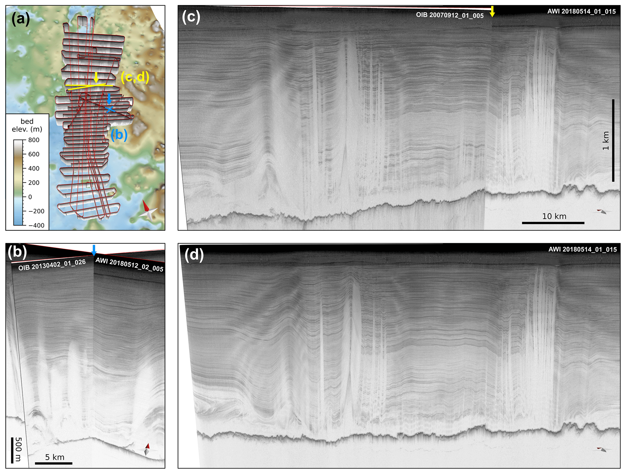
Figure B1Comparison of selected AWI ultra-wideband (UWB) radargrams with OIB radargrams. (a) Three-dimensional view of the EGRIP-NOR-2018 survey highlighting the location of (b) two intersecting radargrams (OIB profile 20130402_01_026 and AWI profile 20180512_02_003; blue lines in a) and (c, d) two nearly parallel-oriented profiles showing both shear margins of NEGIS (OIB profile 20070912_01_005 and AWI profile 20180514_01_015; yellow lines in a). The 2007 OIB radar profile was recorded with the MCRDS (Multi-Channel Radar Depth Sounder) system with a bandwidth of 140–160 MHz and the 2013 profile with the MCoRDS 3 (Multi-Channel Coherent Radar Depth Sounder) system with a bandwidth of 180–210 MHz.
SF, ND, and TAG wrote the manuscript. TB, DJ, and JDP acquired the radar data in the field. OE and DJ were PI and co-PI of the radar campaign. TB and SF processed the radar data with the support of JDP, DJ, VH, and DS. All authors discussed and revised the manuscript.
The contact author has declared that neither they nor their co-authors have any competing interests.
Publisher's note: Copernicus Publications remains neutral with regard to jurisdictional claims in published maps and institutional affiliations.
This article is part of the special issue “Extreme environment datasets for the three poles”. It is not associated with a conference.
We thank the AWI and Kenn Borek crew of the research aircraft Polar 6. Logistical support in the field was provided by the East Greenland Ice-Core Project. EastGRIP is directed and organized by the Centre of Ice and Climate at the Niels Bohr Institute.
EastGRIP is supported by funding agencies and institutions in Denmark (A. P. Møller Foundation, University of Copenhagen), the USA (US National Science Foundation, Office of Polar Programs), Germany (Alfred Wegener Institute, Helmholtz Centre for Polar and Marine Research), Japan (National Institute of Polar Research and Arctic Challenge for Sustainability), Norway (University of Bergen and Bergen Research Foundation), Switzerland (Swiss National Science Foundation), France (French Polar Institute Paul-Emile Victor, Institute for Geosciences and Environmental research), and China (Chinese Academy of Sciences and Beijing Normal University). Support was provided through the use of the CReSIS toolbox from CReSIS, generated with support from the University of Kansas; NASA Operation IceBridge (grant no. NNX16AH54G); and the NSF (grant nos. ACI-1443054, OPP-1739003, and IIS-1838230). Steven Franke was funded by the AWI Strategy Fund and Daniela Jansen by the AWI Strategy Fund and the Helmholtz Young Investigator Group (grant no. HGF YIG VH-NG-802).
This paper was edited by Tao Che and reviewed by Baojun Zhang and one anonymous referee.
Allen, C. T., Mozaffar, S. N., and Akins, T. L.: Suppressing coherent noise in radar applications with long dwell times, IEEE Geoscience and Remote Sens. Lett., 2, 284–286, https://doi.org/10.1109/LGRS.2005.847931, 2005. a
Baldwin, D. J., Bamber, J. L., Payne, A. J., and Layberry, R. L.: Using internal layers from the Greenland ice sheet, identified from radio-echo sounding data, with numerical models, Ann. Glaciol., 37, 325–330, https://doi.org/10.3189/172756403781815438, 2003. a
Bamber, J. L., Griggs, J. A., Hurkmans, R. T. W. L., Dowdeswell, J. A., Gogineni, S. P., Howat, I., Mouginot, J., Paden, J., Palmer, S., Rignot, E., and Steinhage, D.: A new bed elevation dataset for Greenland, The Cryosphere, 7, 499–510, https://doi.org/10.5194/tc-7-499-2013, 2013. a
Blackwell, D. and Richards, M.: Geothermal Map of North America, AAPG Map, scale 1:6 500 000, https://www.smu.edu/Dedman/Academics/Departments/Earth-Sciences/Research/GeothermalLab/DataMaps/GeothermalMapofNorthAmerica (last access: 17 March 2021), 2004. a
Bohleber, P., Wagner, N., and Eisen, O.: Permittivity of ice at radio frequencies: Part II. Artificial and natural polycrystalline ice, Cold Reg. Sci. Technol., 83–84, 13–19, https://doi.org/10.1016/j.coldregions.2012.05.010, 2012. a
Bons, P. D., de Riese, T., Franke, S., Llorens, M.-G., Sachau, T., Stoll, N., Weikusat, I., Westhoff, J., and Zhang, Y.: Comment on “Exceptionally high heat flux needed to sustain the Northeast Greenland Ice Stream” by Smith-Johnsen et al. (2020), The Cryosphere, 15, 2251–2254, https://doi.org/10.5194/tc-15-2251-2021, 2021. a
Buchardt, S. L. and Dahl-Jensen, D.: Estimating the basal melt rate at NorthGRIP using a Monte Carlo technique, Ann. Glaciol., 45, 137–142, https://doi.org/10.3189/172756407782282435, 2007. a
Carter, S. P., Blankenship, D. D., Peters, M. E., Young, D. A., Holt, J. W., and Morse, D. L.: Radar-based subglacial lake classification in Antarctica, Geochem. Geophys. Geosyst., 8, Q03016, https://doi.org/10.1029/2006GC001408, 2007. a
Christianson, K., Peters, L. E., Alley, R. B., Anandakrishnan, S., Jacobel, R. W., Riverman, K. L., Muto, A., and Keisling, B. A.: Dilatant till facilitates ice-stream flow in northeast Greenland, Earth Planet. Sc. Lett., 401, 57–69, https://doi.org/10.1016/j.epsl.2014.05.060, 2014. a, b, c, d
Copland, L. and Sharp, M.: Mapping thermal and hydrological conditions beneath a polythermal glacier with radio-echo sounding, J. Glaciol., 47, 232–242, https://doi.org/10.3189/172756501781832377, 2001. a
CReSIS: CReSIS rds documentation, https://data.cresis.ku.edu/data/rds/rds_readme.pdf (last access: 17 March 2021), 2020a. a, b
CReSIS: CReSIS Toolbox [computer software], Lawrence, Kansas, USA, https://ops.cresis.ku.edu/wiki/index.php/Main_Page (last access: 17 March 2021), 2020b. a, b
Dahl-Jensen, D., Thorsteinsson, T., Alley, R., and Shoji, H.: Flow properties of the ice from the Greenland Ice Core Project ice core: The reason for folds?, J. Geophys. Res.-Oceans, 102, 26831–26840, https://doi.org/10.1029/97JC01266, 1997. a
Eder, K., Reidler, C., Mayer, C., and Leopold, M.: Crevasse detection in alpine areas using ground penetrating radar as a component for a mountain guide system, International Archives of the Photogrammetry, Remote Sensing and Spatial Information Sciences – ISPRS Archives, 37, 837–842, 2008. a
Eisen, O., Hamann, I., Kipfstuhl, S., Steinhage, D., and Wilhelms, F.: Direct evidence for continuous radar reflector originating from changes in crystal-orientation fabric, The Cryosphere, 1, 1–10, https://doi.org/10.5194/tc-1-1-2007, 2007. a
Eisen, O., Franke, S., Jansen, D., Paden, J., Drews, R., Ershadi, M. R., Steinhage, D., Lilien, D., Yan, J., Weikusat, I., Wilhelms, F., Dahl-Jensen, D., Grindsted, A., Hvidberg, C., and Miller, H.: Fabric beats in radar data across the NEGIS ice stream, EGU General Assembly 2021, online, 19–30 April 2021, EGU21-1207, https://doi.org/10.5194/egusphere-egu21-1207, 2021. a
Fahnestock, M., Bindschadler, R., Kwok, R., and Jezek, K.: Greenland Ice Sheet surface properties and ice dynamics from ERS-1 SAR imagery, Science, 262, 1530–1534, https://doi.org/10.1126/science.262.5139.1530, 1993. a
Fahnestock, M. A., Joughin, I., Scambos, T. A., Kwok, R., Krabill, W. B., and Gogineni, S.: Ice-stream-related patterns of ice flow in the interior of northeast Greenland, J. Geophys. Res.-Atmos., 106, 34035–34045, https://doi.org/10.1029/2001JD900194, 2001. a, b, c
Franke, S., Jansen, D., Binder, T., Dörr, N., Paden, J., Helm, V., Steinhage, D., and Eisen, O.: Bedrock topography and ice thickness in the onset region of the Northeast Greenland Ice Stream recorded with the airborne AWI Ultra-Wideband radar (UWB) in 2018, PANGAEA [data set], https://doi.org/10.1594/PANGAEA.907918, 2019. a, b
Franke, S., Jansen, D., Binder, T., Dörr, N., Helm, V., Paden, J., Steinhage, D., and Eisen, O.: Bed topography and subglacial landforms in the onset region of the Northeast Greenland Ice Stream, Ann. Glaciol., 61, 143–153, https://doi.org/10.1017/aog.2020.12, 2020. a, b, c, d, e, f, g, h
Franke, S., Binder, T., Jansen, D., Paden, J. D., Dörr, N., Gerber, T., Miller, H., Dahl-Jensen, D., Helm, V., Steinhage, D., Weikusat, I., Wilhelms, F., and Eisen, O.: Ultra-wideband radar data over the shear margins and along flow lines at the onset region of the Northeast Greenland Ice Stream (NEGIS), PANGAEA [data set], https://doi.org/10.1594/PANGAEA.928569, 2021a. a, b, c
Franke, S., Eisermann, H., Jokat, W., Eagles, G., Asseng, J., Miller, H., Steinhage, D., Helm, V., Eisen, O., and Jansen, D.: Preserved landscapes underneath the Antarctic Ice Sheet reveal the geomorphological history of Jutulstraumen Basin, Earth Surf. Process. Landf., 46, 2728–2745, https://doi.org/10.1002/esp.5203, 2021b. a
Franke, S., Jansen, D., Beyer, S., Neckel, N., Binder, T., Paden, J., and Eisen, O.: Complex Basal Conditions and Their Influence on Ice Flow at the Onset of the Northeast Greenland Ice Stream, J. Geophys. Res.-Earth Surf., 126, e2020JF005689, https://doi.org/10.1029/2020JF005689, 2021c. a, b, c, d
Frezzotti, M., Gandolfi, S., and Urbini, S.: Snow megadunes in Antarctica: Sedimentary structure and genesis, J. Geophys. Res.-Atmos., 107, ACL 1-1–ACL 1-12, https://doi.org/10.1029/2001JD000673, 2002. a
Fujita, S., Maeno, H., Uratsuka, S., Furukawa, T., Mae, S., Fujii, Y., and Watanabe, O.: Nature of radio echo layering in the Antarctic ice sheet detected by a two-frequency experiment, J. Geophys. Res.-Sol. Ea., 104, 13013–13024, https://doi.org/10.1029/1999jb900034, 1999. a
Gazdag, J.: Wave equation migration with the phase‐shift method, Geophysics, 43, 1342–1351, https://doi.org/10.1190/1.1440899, 1978. a
Gerber, T. A., Hvidberg, C. S., Rasmussen, S. O., Franke, S., Sinnl, G., Grinsted, A., Jansen, D., and Dahl-Jensen, D.: Upstream flow effects revealed in the EastGRIP ice core using Monte Carlo inversion of a two-dimensional ice-flow model, The Cryosphere, 15, 3655–3679, https://doi.org/10.5194/tc-15-3655-2021, 2021. a, b
Gogineni, S., Chuah, T., Allen, C., Jezek, K., and Moore, R. K.: An improved coherent radar depth sounder, J. Glaciol., 44, 659–669, https://doi.org/10.3189/S0022143000002161, 1998. a
Hale, R., Miller, H., Gogineni, S., Yan, J. B., Rodriguez-Morales, F., Leuschen, C., Paden, J., Li, J., Binder, T., Steinhage, D., Gehrmann, M., and Braaten, D.: Multi-channel ultra-wideband radar sounder and imager, in: 2016 IEEE International Geoscience and Remote Sensing Symposium (IGARSS), 10–15 July 2016, Beijing, China, 2112–2115, https://doi.org/10.1109/IGARSS.2016.7729545, 2016. a
Hempel, L. and Thyssen, F.: Deep radio echo soundings in the vicinity of GRIP and GISP2 drill sites, Greenland, Polarforschung, 62, 11–16, 1992. a
Hempel, L., Thyssen, F., Gundestrup, N., Clausen, H. B., and Miller, H.: A comparison of radio-echo sounding data and electrical conductivity of the GRIP ice core, J. Glaciol., 46, 369–374, https://doi.org/10.3189/172756500781833070, 2000. a
Hodgkins, R., Siegert, M. J., and Dowdeswell, J. A.: Geophysical investigations of ice-sheet internal layering and deformation in the Dome C region of central East Antarctica, J. Glaciol., 46, 161–166, https://doi.org/10.3189/172756500781833223, 2000. a
Holschuh, N., Christianson, K., and Anandakrishnan, S.: Power loss in dipping internal reflectors, imaged using ice-penetrating radar, Ann. Glaciol., 55, 49–56, https://doi.org/10.3189/2014aog67a005, 2014. a
Holschuh, N., Lilien, D. A., and Christianson, K.: Thermal Weakening, Convergent Flow, and Vertical Heat Transport in the Northeast Greenland Ice Stream Shear Margins, Geophys. Res. Lett., 46, 8184–8193, https://doi.org/10.1029/2019GL083436, 2019. a
Huybrechts, P., Steinhage, D., Wilhelms, F., and Bamber, J.: Balance velocities and measured properties of the Antarctic ice sheet from a new compilation of gridded data for modelling, Ann. Glaciol., 30, 52–60, https://doi.org/10.3189/172756400781820778, 2000. a
Jacobel, R. W. and Hodge, S. M.: Radar internal layers from the Greenland Summit, Geophys. Res. Lett., 22, 587–590, https://doi.org/10.1029/95GL00110, 1995. a
Jacobel, R. W., Gades, A. M., Gottschling, D. L., Hodge, S. M., and Wright, D. L.: Interpretation of radar-detected internal layer folding in West Antarctic ice streams, J. Glaciol., 39, 528–537, https://doi.org/10.1017/s0022143000016427, 1993. a
Jóhannesson, T., Pálmason, B., Hjartarson, A., Jarosch, A. H., Magnússon, E., Belart, J. M. C., and Gudmundsson, M. T.: Non-surface mass balance of glaciers in Iceland, J. Glaciol., 66, 685–697, https://doi.org/10.1017/jog.2020.37, 2020. a
Jordan, T. M., Schroeder, D. M., Elsworth, C. W., and Siegfried, M. R.: Estimation of ice fabric within Whillans Ice Stream using polarimetric phase-sensitive radar sounding, Ann. Glaciol., 61, 74–83, https://doi.org/10.1017/aog.2020.6, 2020. a
Joughin, I., Fahnestock, M., MacAyeal, D., Bamber, J. L., and Gogineni, P.: Observation and analysis of ice flow in the largest Greenland ice stream, J. Geophys. Res. Atmos., 106, 34021–34034, https://doi.org/10.1029/2001JD900087, 2001. a, b, c
Joughin, I., Smith, B., Howat, I., and Scambos, T.: MEaSUREs Greenland Ice Sheet Velocity Map from InSAR Data, Version 2, Boulder, Colorado USA, NASA National Snow and Ice Data Center Distributed Active Archive Center [data set], https://doi.org/10.5067/OC7B04ZM9G6Q, 2015, updated 2018. a
Joughin, I., Smith, B. E., and Howat, I. M.: A complete map of Greenland ice velocity derived from satellite data collected over 20 years, J. Glaciol., 64, 1–11, https://doi.org/10.1017/jog.2017.73, 2017. a, b, c, d
Kanagaratnam, P., Gogineni, S. P., Gundestrup, N., and Larsen, L.: High-resolution radar mapping of internal layers at the North Greenland Ice Core Project, J. Geophys. Res.-Atmos., 106, 33799–33811, https://doi.org/10.1029/2001JD900191, 2001. a
Keisling, B. A., Christianson, K., Alley, R. B., Peters, L. E., Christian, J. E., Anandakrishnan, S., Riverman, K. L., Muto, A., and Jacobel, R. W.: Basal conditions and ice dynamics inferred from radar-derived internal stratigraphy of the northeast Greenland ice stream, Ann. Glaciol., 55, 127–137, https://doi.org/10.3189/2014AoG67A090, 2014. a, b, c
Leuschen, C., Gogineni, S., and Tammana, D.: SAR processing of radar echo sounder data, in: IGARSS 2000. IEEE 2000 International Geoscience and Remote Sensing Symposium. Taking the Pulse of the Planet: The Role of Remote Sensing in Managing the Environment. Proceedings (Cat. No.00CH37120), 6, 2570–2572, https://doi.org/10.1109/IGARSS.2000.859643, 2000. a
Li, J., Paden, J., Leuschen, C., Rodriguez-Morales, F., Hale, R. D., Arnold, E. J., Crowe, R., Gomez-Garcia, D., and Gogineni, P.: High-Altitude Radar Measurements of Ice Thickness Over the Antarctic and Greenland Ice Sheets as a Part of Operation IceBridge, IEEE T. Geosci. Remote, 51, 742–754, https://doi.org/10.1109/TGRS.2012.2203822, 2013. a
Lilien, D. A., Rathmann, N. M., Hvidberg, C. S., and Dahl-Jensen, D.: Modeling Ice-Crystal Fabric as a Proxy for Ice-Stream Stability, J. Geophys. Res.-Earth Surf., 126, e2021JF006306, https://doi.org/10.1029/2021JF006306, 2021. a
MacGregor, J. A., Fahnestock, M. A., Catania, G. A., Aschwanden, A., Clow, G. D., Colgan, W. T., Gogineni, S. P., Morlighem, M., Nowicki, S. M., Paden, J. D., Price, S. F., and Seroussi, H.: A synthesis of the basal thermal state of the Greenland Ice Sheet, J. Geophys. Res.-Earth Surf., 121, 1328–1350, https://doi.org/10.1002/2015JF003803, 2016. a
Matsuoka, K., Furukawa, T., Fujita, S., Maeno, H., Uratsuka, S., Naruse, R., and Watanabe, O.: Crystal orientation fabrics within the Antarctic ice sheet revealed by a multipolarization plane and dual-frequency radar survey, J. Geophys. Res.-Sol. Ea., 108, 2499, https://doi.org/10.1029/2003jb002425, 2003. a
Millar, D. H.: Radio-echo layering in polar ice sheets and past volcanic activity, Nature, 292, 441–443, https://doi.org/10.1038/292441a0, 1981. a
Mottram, R., Simonsen, S. B., Svendsen, S. H., Barletta, V. R., Sørensen, L. S., Nagler, T., Wuite, J., Groh, A., Horwath, M., Rosier, J., Solgaard, A., Hvidberg, C. S., and Forsberg, R.: An integrated view of greenland ice sheet mass changes based on models and satellite observations, Remote Sens., 11, 1–26, https://doi.org/10.3390/rs11121407, 2019. a
Murray, T., Stuart, G. W., Miller, P. J., Woodward, J., Smith, A. M., Porter, P. R., and Jiskoot, H.: Glacier surge propagation by thermal evolution at the bed, J. Geophys. Res.-Sol. Ea., 105, 13491–13507, https://doi.org/10.1029/2000jb900066, 2000. a
Nereson, N. A. and Raymond, C. F.: The elevation history of ice streams and the spatial accumulation pattern along the Siple Coast of West Antarctica inferred from ground-based radar data from three inter-ice-stream ridges, J. Glaciol., 47, 303–313, https://doi.org/10.3189/172756501781832197, 2001. a
Nereson, N. A., Raymond, C. F., Jacobel, R. W., and Waddington, E. D.: The accumulation pattern across Siple Dome, West Antarctica, inferred from radar-detected internal layers, J. Glaciol., 46, 75–87, https://doi.org/10.3189/172756500781833449, 2000. a
Nixdorf, U. and Göktas, F.: Spatial depth distribution of the subglacial bed and internal layers in the ice around NGRIP, Greenland, derived with airborne RES, J. Appl. Geophys., 47, 175–182, https://doi.org/10.1016/S0926-9851(01)00062-3, 2001. a
Pälli, A., Kohler, J. C., Isaksson, E., Moore, J. C., Pinglot, J. F., Pohjola, V. A., and Samuelsson, H.: Spatial and temporal variability of snow accumulation using ground-penetrating radar and ice cores on a Svalbard glacier, J. Glaciol., 48, 417–424, https://doi.org/10.3189/172756502781831205, 2002. a, b
Palmer, S. J., Dowdeswell, J. A., Christoffersen, P., Young, D. A., Blankenship, D. D., Greenbaum, J. S., Benham, T., Bamber, J., and Siegert, M. J.: Greenland subglacial lakes detected by radar, Geophys. Res. Lett., 40, 6154–6159, https://doi.org/10.1002/2013GL058383, 2013. a
Richardson, C., Aarholt, E., Hamran, S.-E., Holmlund, P., and Isaksson, E.: Spatial distribution of snow in western Dronning Maud Land, East Antarctica, mapped by a ground-based snow radar, J. Geophys. Res., 102, 20343–20353, 1997. a
Rignot, E. and Mouginot, J.: Ice flow in Greenland for the International Polar Year 2008-2009, Geophys. Res. Lett., 39, L11501, https://doi.org/10.1029/2012GL051634, 2012. a
Riverman, K. L., Alley, R. B., Anandakrishnan, S., Christianson, K., Holschuh, N. D., Medley, B., Muto, A., and Peters, L. E.: Enhanced Firn Densification in High‐Accumulation Shear Margins of the NE Greenland Ice Stream, J. Geophys. Res.-Earth Surf., 124, 365–382, https://doi.org/10.1029/2017JF004604, 2019a. a, b
Riverman, K. L., Anandakrishnan, S., Alley, R. B., Holschuh, N., Dow, C. F., Muto, A., Parizek, B. R., Christianson, K., and Peters, L. E.: Wet subglacial bedforms of the NE Greenland Ice Stream shear margins, Ann. Glaciol., 60, 91–99, https://doi.org/10.1017/aog.2019.43, 2019b. a
Schroeder, D. M., Bingham, R. G., Blankenship, D. D., Christianson, K., Eisen, O., Flowers, G. E., Karlsson, N. B., Koutnik, M. R., Paden, J. D., and Siegert, M. J.: Five decades of radioglaciology, Ann. Glaciol., 61, 1–13, https://doi.org/10.1017/aog.2020.11, 2020. a
Shepherd, A., Ivins, E., Rignot, E., Smith, B., van den Broeke, M., Velicogna, I., Whitehouse, P., Briggs, K., Joughin, I., Krinner, G., Nowicki, S., Payne, T., Scambos, T., Schlegel, N., A, G., Agosta, C., Ahlstrøm, A., Babonis, G., Barletta, V. R., Bjørk, A. A., Blazquez, A., Bonin, J., Colgan, W., Csatho, B., Cullather, R., Engdahl, M. E., Felikson, D., Fettweis, X., Forsberg, R., Hogg, A. E., Gallee, H., Gardner, A., Gilbert, L., Gourmelen, N., Groh, A., Gunter, B., Hanna, E., Harig, C., Helm, V., Horvath, A., Horwath, M., Khan, S., Kjeldsen, K. K., Konrad, H., Langen, P. L., Lecavalier, B., Loomis, B., Luthcke, S., McMillan, M., Melini, D., Mernild, S., Mohajerani, Y., Moore, P., Mottram, R., Mouginot, J., Moyano, G., Muir, A., Nagler, T., Nield, G., Nilsson, J., Noël, B., Otosaka, I., Pattle, M. E., Peltier, W. R., Pie, N., Rietbroek, R., Rott, H., Sandberg Sørensen, L., Sasgen, I., Save, H., Scheuchl, B., Schrama, E., Schröder, L., Seo, K. W., Simonsen, S. B., Slater, T., Spada, G., Sutterley, T., Talpe, M., Tarasov, L., van de Berg, W. J., van der Wal, W., van Wessem, M., Vishwakarma, B. D., Wiese, D., Wilton, D., Wagner, T., Wouters, B., and Wuite, J.: Mass balance of the Greenland Ice Sheet from 1992 to 2018, Nature, 579, 233–239, https://doi.org/10.1038/s41586-019-1855-2, 2020. a
Siegert, M. J. and Hodgkins, R.: A stratigraphic link across 1100 km of the antarctic ice sheet between the Vostok ice-core site and Titan Dome (near South Pole), Geophys. Res. Lett., 27, 2133–2136, https://doi.org/10.1029/2000GL008479, 2000. a
Siegert, M. J., Hodgkins, R., and Dowdeswell, J. A.: A chronology for the Dome C deep ice-core site through radio-echo layer correlation with the Vostok ice core, Antarctica, Geophys. Res. Lett., 25, 1019–1022, https://doi.org/10.1029/98GL00718, 1998. a
Smith-Johnsen, S., Schlegel, N.-J., de Fleurian, B., and Nisancioglu, K. H.: Sensitivity of the Northeast Greenland Ice Stream to Geothermal Heat, J. Geophys. Res.-Earth Surf., 125, e2019JF005252, https://doi.org/10.1029/2019JF005252, 2020. a
Steinhage, D., Nixdorf, U., Meyer, U., and Miller, H.: New maps of the ice thickness and subglacial topography in Dronning Maud Land, Antarctica, determined by means of airborne radio-echo sounding, Ann. Glaciol., 29, 267–272, https://doi.org/10.3189/172756499781821409, 1999. a, b
Straneo, F., Sutherland, D. A., Holland, D., Gladish, C., Hamilton, G. S., Johnson, H. L., Rignot, E., Xu, Y., and Koppes, M.: Characteristics of ocean waters reaching Greenland's glaciers, Ann. Glaciol., 53, 202–210, https://doi.org/10.3189/2012AoG60A059, 2012. a
Vallelonga, P., Christianson, K., Alley, R. B., Anandakrishnan, S., Christian, J. E. M., Dahl-Jensen, D., Gkinis, V., Holme, C., Jacobel, R. W., Karlsson, N. B., Keisling, B. A., Kipfstuhl, S., Kjær, H. A., Kristensen, M. E. L., Muto, A., Peters, L. E., Popp, T., Riverman, K. L., Svensson, A. M., Tibuleac, C., Vinther, B. M., Weng, Y., and Winstrup, M.: Initial results from geophysical surveys and shallow coring of the Northeast Greenland Ice Stream (NEGIS), The Cryosphere, 8, 1275–1287, https://doi.org/10.5194/tc-8-1275-2014, 2014. a, b
Vaughan, D. G., Corr, H. F., Doake, C. S., and Waddington, E. D.: Distortion of isochronous layers in ice revealed by ground-penetrating radar, Nature, 398, 323–326, https://doi.org/10.1038/18653, 1999. a
Wang, Z., Gogineni, S., Rodriguez-Morales, F., Yan, J.-B., Paden, J., Leuschen, C. Hale, R. D., Li, J., Carabajal, L. C., Gomez-Garcia, D., Townley, B., Willer, R., Stearns, L., Child, S., and Braaten, D.: Multichannel Wideband Synthetic Aperture Radar for Ice Sheet Remote Sensing: Development and the First Deployment in Antarctica, IEEE J. Sel. Top. Appl., 9, 1–28, https://doi.org/10.1109/JSTARS.2015.2403611, 2015. a
Westhoff, J., Stoll, N., Franke, S., Weikusat, I., Bons, P., Kerch, J., Jansen, D., Kipfstuhl, S., and Dahl-Jensen, D.: A stratigraphy-based method for reconstructing ice core orientation, Ann. Glaciol., 62, 191–202, https://doi.org/10.1017/aog.2020.76, 2020. a
Williams, R. M., Ray, L. E., Lever, J. H., and Burzynski, A. M.: Crevasse detection in ice sheets using ground penetrating radar and machine learning, IEEE J. Sel. Top. Appl., 7, 4836–4848, https://doi.org/10.1109/JSTARS.2014.2332872, 2014. a
Yin, J., Overpeck, J. T., Griffies, S. M., Hu, A., Russell, J. L., and Stouffer, R. J.: Different magnitudes of projected subsurface ocean warming around Greenland and Antarctica, Nat. Geosci., 4, 524–528, https://doi.org/10.1038/nphys1189, 2011. a
Young, D. A., Schroeder, D. M., Blankenship, D. D., Kempf, S. D., and Quartini, E.: The distribution of basal water between Antarctic subglacial lakes from radar sounding, Philos. T. R. Soc. A, 374, https://doi.org/10.1098/rsta.2014.0297, 2016. a
Young, T. J., Schroeder, D. M., Jordan, T. M., Christoffersen, P., Tulaczyk, S. M., Culberg, R., and Bienert, N. L.: Inferring Ice Fabric From Birefringence Loss in Airborne Radargrams: Application to the Eastern Shear Margin of Thwaites Glacier, West Antarctica, J. Geophys. Res.-Earth Surf., 126, e2020JF006023, https://doi.org/10.1029/2020JF006023, 2021. a
Zamora, R., Casassa, G., Rivera, A., Ordenes, F., Neira, G., Araya, L., Mella, R., and Bunster, C.: Crevasse detection in glaciers of southern Chile and Antarctica by means of ground penetrating radar, IAHS-AISH Publication, 153–162, 2007. a
Zeising, O. and Humbert, A.: Indication of high basal melting at the EastGRIP drill site on the Northeast Greenland Ice Stream, The Cryosphere, 15, 3119–3128, https://doi.org/10.5194/tc-15-3119-2021, 2021. a
- Abstract
- Introduction
- Survey region and previous work
- Methods
- Results
- Relevance of the data set
- Code and data availability
- Conclusions
- Appendix A: Additional information for the segments
- Appendix B: Comparison to OIB surveys
- Author contributions
- Competing interests
- Disclaimer
- Special issue statement
- Acknowledgements
- Financial support
- Review statement
- References